Systematic Review

Beyond In Situ Measurements: Systematic Review of Satellite-Based Approaches for Monitoring Dissolved Oxygen Concentrations in Global Surface Waters

by
Irene Biliani
and
Ierotheos Zacharias
*
Laboratory of Environmental Engineering, Department of Civil Engineering, University of Patras, 26205 Patras, Greece
*
Author to whom correspondence should be addressed.
Remote Sens. 2026, 18(3), 428; https://doi.org/10.3390/rs18030428
Submission received: 5 December 2025 / Revised: 17 January 2026 / Accepted: 26 January 2026 / Published: 29 January 2026

Highlights

What are the main findings?
  • Satellite remote sensing can effectively estimate surface dissolved oxygen using empirical, semi-empirical, machine learning, and deep learning approaches.
  • Machine learning and deep learning models significantly improve DO prediction when supported by high-quality in situ data.
What are the implications of the main findings?
  • Remote sensing DO estimation enables large-scale, cost-effective monitoring of hypoxia, eutrophication, and deoxygenation.
  • Reliable application requires rigorous validation and continuous recalibration with field observations.

Abstract

Dissolved oxygen (DO) is a cornerstone of aquatic ecosystem vitality, yet conventional in situ monitoring methods, reliant on field probes, buoys, and lab analyses, struggle to capture the spatiotemporal variability of DO at regional or global scales. Satellite remote sensing has revolutionized water quality assessment by enabling systematic, high-frequency, and spatially continuous monitoring of surface waters, transcending the logistical and financial constraints of traditional approaches. This systematic review critically evaluates satellite-based methodologies for estimating DO concentrations, emphasizing their capacity to address global environmental challenges such as eutrophication, hypoxia, and climate-driven deoxygenation. Following the PRISMA 2020 guidelines, large bibliographic databases (Scopus, Web of Science, and Google Scholar) identified that studies on satellite-derived DO concentrations are focused on both spectral and thermal foundations of DO retrieval, including empirical relationships with proxy variables (e.g., Chlorophyll-a, sea surface temperature, and turbidity) as well as direct optical signatures linked to oxygen absorption in the red and near-infrared spectra. The 77 results included in this review (accessed on 27 November 2025) indicate that the reported advances in sensor technologies (e.g., Sentinel-2,3’s OLCI and MODIS) have greatly expanded the ability to monitor DO levels across different types of water bodies, and that there has been a significant paradigm shift towards more complex and sophisticated machine learning and deep learning architectures. Recent work demonstrates that advanced machine learning and deep learning models can effectively estimate DO from remote sensing proxies, achieving high predictive performance when validated against in situ observations. Overall, this review indicates that their effectiveness depends heavily on high-quality training data, rigorous validation, and careful recalibration. Global case studies illustrate applications showcasing the scalability of remote sensing solutions. An OSF project was created to enhance transparency, while the review protocol was not prospectively registered, which is consistent with the PRISMA 2020 guidelines for non-registered reviews.

1. Introduction

Dissolved oxygen (DO) in water bodies is a crucial factor that controls the health of the overall aquatic ecosystem. The concentration of oxygen dissolved in a water body is determined by the equilibrium/balance between the process of production of organic matter (from photosynthesis) and the process of consumption of that same organic matter (through respiration) [1,2]. Global warming is profoundly reshaping the oxygen balance in aquatic ecosystems. As the climate’s temperature increases, the warmer ocean water reduces the amount of dissolved oxygen, while the rate of microbial respiration, nitrification, and sediment oxygen consumption increases, promoting longer and more intense thermal stratification. This combination of factors results in diminished vertical mixing and reduced bottom water ventilation, leading to stratified lakes, coastal areas, and estuaries. A decline in surface DO levels indicates that water bodies enter the early stages of the eutrophication, which leads to the death of millions of fish, the loss of biodiversity, the collapse of fisheries [3], and overall water quality deterioration. When the DO concentration falls below 2 mg/L, “hypoxic” conditions are created that stress the health of the species within the aquatic environment, culminating in mass mortality when DO falls below 0.5 mg/L, leading to what is known as “anoxia” [4], which has major ecological and socioeconomic consequences [5]. Other terms used to describe anoxic or “hypoxic” conditions are “Dead Coastal Zones”, “Oxygen-Depleted areas” or Oxygen Minimum Zones (OMZs) [6]. Anoxic and hypoxic areas can be found scattered across the globe, are characteristic of areas with high population density combined with increased use of industrially produced nitrogen fertilizers since the late 1940s [7]. Typical examples of such areas are the Adriatic, the Black Sea, the Baltic Sea, the Gulf of Mexico, and the East China Sea [8], all of which are important fishing areas.
The concentration of dissolved oxygen found in coastal areas, seas, and oceans is highly correlated with SST and Chl-a concentrations, therefore relating physical factors to biological productivity and to suitable habitats for spawning and feeding [9]. It has been proven that a 1 °C increase in global temperatures will decrease the solubility of oxygen in the world’s oceans and may also contribute to increased stratification, thus further decreasing DO [1]. Similar correlations exist within freshwater systems; in these systems DO represents the balance between oxygen produced through photosynthesis and oxygen consumed through respiration due to the organic load present in the water and it affects the suitability of the water for drinking, irrigation, and aquaculture [3]. Therefore, DO data across an entire basin is critical for managing fisheries, assessing ecosystem services, and quantifying the climate-induced changes to global biogeochemical cycles [10].
Traditional monitoring systems, using probes, buoys, and lab tests, provide accurate data at specific locations; however, these systems are very costly and provide limited spatial detail [11,12]. Large rivers, lakes, and ocean margins have too few in situ stations to accurately record the strong spatial variations in DO levels, especially where there are sharp DO distributions, such as river mouth plumes or the edges of hypoxic zones [9,12]. Additionally, the temporal resolution of these stations is typically low, so the fast-changing nature of DO, as during storm events or algal blooms, may be missed by monthly or seasonal sampling [13]. Additionally, due to the high cost of in situ data, the size of long-term monitoring networks is restricted and therefore there are significant data gaps in DO monitoring in data-poor regions, including large parts of the Indian Ocean, the southern Adriatic Sea, and inland waters of developing countries [14,15]. Furthermore, the logistics of continuous observation in remote and turbid water bodies limit the frequency of DO measurements and therefore the capability of observing how ecosystems respond to environmental stressors [16,17]. Therefore, the lack of systematic, frequent, and contiguous DO data across regional to global scales creates a validation gap between field-measured DO levels and remotely sensed DO products, creating a need to develop new remote sensing techniques to measure DO at the scale required [11,12,13,17].
The transition from point-based water quality monitoring to global surface water body analysis requires monitoring large areas of surface waters, enabling the concept of “beyond in situ”. In situ measurements can be used in conjunction with remote sensing (RS) data to enhance localized efforts. RS has three main advantages over traditional in situ methods and is therefore used to scale-up the in situ measurements to obtain a spatial synoptic view, temporal frequency, and long-term consistency. Satellites (Sentinel, MODIS, etc.) allow for continued and broad area observation of DO and other water quality parameters in addition to allowing for the observation of DO’s temporal and spatial distribution, which cannot be captured using single-point in situ measurements [11,18,19]. This allows for the development of high-resolution DO data and other water quality parameters necessary for characterization of regions. Additionally, RS through the study of long-term time series and each water body special characteristics allows for the identification of long-term environmental trends such as deoxygenation [3,20]. Combining the high-accuracy in situ measurements for calibration purposes with wide coverage satellite observations enables the production of cost-effective, continuous, and robust global water quality DO products (trends, phenologies, alarms etc.) [10,21].
Although, the dissolved oxygen is characterized as a non-optically active parameter, over the last 5 years, the rapid development of remote sensing applications to develop methodologies for dissolved oxygen concentrations/levels retrieval has been remarkable. The three primary approaches to estimating dissolved oxygen (DO) include empirical, semi-empirical, and machine learning/artificial intelligence (ML/AI) methods [22,23,24]. Because DO does not respond spectrally, indirect estimation of DO is established through linkage with strong optically active parameters (OAPs) such as Chlorophyll-a (Chl-a) and sea surface temperature (SST) [1,25]. Empirical and semi-empirical models utilize regression analysis using either spectral bands or band ratios to establish these correlations [22]. Advanced ML models such as random forest (RF) and support vector regression (SVR) demonstrate better estimates of DO in cost of complexity with the application of non-linear models [24,26].
The scope of this review is to assess remote sensing applications for determining dissolved oxygen concentration of surface water bodies. Although all water body types have been reviewed, including inland water bodies, marines, seas, and oceans, there is a greater emphasis on inland waters such as lakes, rivers, and coastal areas, since they represent the majority of water bodies type, where in situ measurements have been conducted to validate the approach developed. This study aims to highlight innovative algorithmic techniques that can effectively analyze remote sensing data to provide accurate oxygen concentrations.

2. Materials and Methods

A systematic literature review was performed to synthesize existing knowledge on the algorithmic approaches developed for satellite-derived dissolved oxygen concentrations in the aquatic environment. The literature search was carried out using the Scopus, Web of Science, and Google Scholar academic databases, and included peer-review articles, excluding conference proceedings and technical reports. The search included articles published from 2015 to the present (27 November 2025) in an effort to include recent advances consisting of 77 published papers. The search of the scientific literature included the following keywords: “oxygen”, “dissolved oxygen”, “remote sensing”, “algorithms”, “models”, “satellite”, “imagery”, “deoxygenation”, “spatiotemporal”, “oceanographic monitoring”, “algorithm” “retrieval”, “estimate”, “predict”, “machine learning”, and “circulation”. Search queries were later refined to obtain the most relevant studies focusing on water quality and not on terrestrial management or the biological characteristics of fisheries. Finally, the study was limited to the English language and to articles using satellite-derived measurements to obtain DO concentrations. For instance, studies where dissolved oxygen concentrations resulted from numerical models were not included in the dataset. The review identified several extant limitations and barriers to the use of remote sensing technologies to estimate DO levels globally. The PRISMA 2020 flow diagram in Figure 1 presents in detail the datasets used and the inclusion and exclusion criteria. For the needs of the systematic review a Project on the platform of the Open Science Framework for Systematic Reviews has been created, including files that are presented in this manuscript, using the Mendeley Desktop tool (version 1.19.8, Mendeley Ltd., London, UK).

3. State of the Art

3.1. Key Drivers and Dynamics of the Dissolved Oxygen Variability in the Aquatic Environment

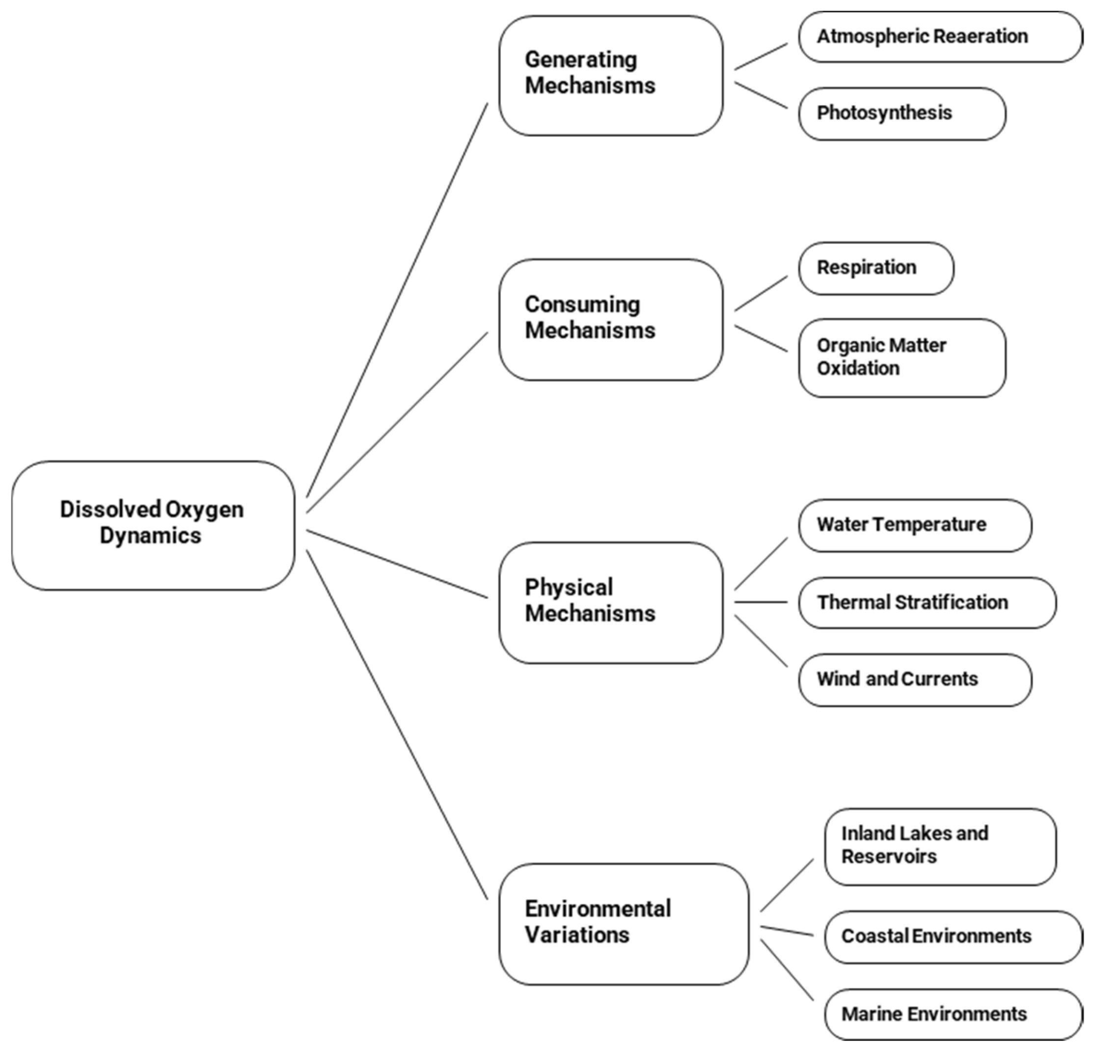
Dissolved oxygen (DO) is a crucial biogeochemical parameter that supports aerobic metabolism, governs organic matter oxidation, and underlies ecosystem health in the aquatic environment [10,27,28]. The concentration of DO is indicative of the balance between DO generating mechanisms (notably atmospheric reaeration and photosynthesis through phytoplankton or macrophytes [27]), and DO-consuming mechanisms (such as respiration by fauna and microorganisms [29]). Physical mechanisms also influence this equilibrium; notably, changes in water temperature decrease the solubility of gases, thereby decreasing DO levels [30], and thermally induced stratification decreases the vertical mixing of water masses, thus creating conditions whereby deeper waters (hypolimnion zone) are isolated from surface oxygen inputs [31]. Conversely, atmosphere wind and currents intensify water column mixing and increase reaeration and redistribution of oxygen [32]. Figure 2 schematic diagram presents the mechanisms that control Dissolved Oxygen in the aquatic environment. For example, DO dynamics within inland lakes and reservoirs are generally influenced by seasonal thermal stratification and local productivity; therefore, DO levels at the surface may reach elevated concentrations in late spring due to the presence of algal blooms, but become depleted at the hypolimnion zone during summer [13]. Furthermore, dissolved oxygen concentration fluctuates in the coastal environments due to the presence of freshwater input, nutrient loading, and tidal exchange, which can create rapid changes in the dissolved oxygen concentrations. Marine environments are characterized by large-scale physical processes (e.g., sea surface temperature or salinity), morphological differences (e.g., bathymetry peculiarities and narrow or large open boundaries) and catchment-dependent anthropogenic activities, which alter the vertical and horizontal distribution of DO and often result in large oxygen-depleted zones [3,10].

3.2. Remote Sensing of Optical and Thermal Properties Relevant to DO Retrieval

Remote sensing analysis for monitoring surface water quality at a very large scale and with frequent sampling has dramatically evolved. Understanding how the physical and optical properties of water interact with solar radiation is important to effectively use remote sensing technologies for water quality monitoring; this includes knowing what water quality parameters can be classified based on optical and thermal properties, and the capabilities of each type of sensor used for remote sensing. Water quality parameters exhibit different types of interaction with satellite sensors’ electromagnetic radiation. Optically active parameters (i.e., Chlorophyll-a, turbidity, total suspended solids (TSS), and colored dissolved organic material (CDOM)) directly affect absorption and scattering of solar radiation signals, producing measurable changes in water-leaving radiance that can be measured with satellite-borne sensors [30]. Optically active parameters are generally retrieved from spectral bands in the visible and near-infrared region, which represent the area of maximum sensitivity of these optically active parameters [33,34,35].
Optically inactive parameters such as dissolved oxygen (DO), total nitrogen (TN), total phosphorus (TP), and chemical oxygen demand (COD) do not have a “straight forward” effect on the optical properties of water and therefore have no measurable “spectral signature/identity”. Nonetheless, after implementation of empirical, semi-empirical, statistical, and machine learning approaches, their concentration may be inferred by applying either correlations between optically active parameters and/or environmental proxies (e.g., water temperature or Chlorophyll-a), or as “secondary resulting” variables (e.g., ratios of specific spectral bands or surface temperature) often complemented with sparse in situ DO measurements [1,36,37]. Specifically for DO, the indirect methods applied exploit other optically active constituents (OACs), which have been linked to oxygen generation (photosynthesis) and oxygen consumption (respiration and decomposition), and usually include Chlorophyll-a (Chl-a) [38], suspended particulate matter (SPM), total suspended solids (TSS) [21], and colored dissolved organic matter (CDOM) [22].
Chlorophyll-a (Chl-a) is the most crucial parameter to quantify and assess algal blooms, and therefore the presence of eutrophication that indicates the potential to reach oxygen generation capacity within the aquatic environment [3,39]. Chl-a concentrations are retrieved by spectral channels found at the wavelengths of 550–580 nm and 700 nm for reflection, and of 438 and 676 nm for absorption [21]. Suspended particulate matter (SPM)/total suspended solids (TSS): SPM can affect light penetration into the water column, thereby influencing photosynthesis. Additionally, SPM can serve as an indicator of adsorption of organic material and subsequent biochemical degradation of organic material, both of which consume oxygen [21]. Typically, high levels of SPM will result in increased reflectance in the red and near-infrared (NIR) portions of the spectrum [40]. Finally, colored dissolved organic matter (CDOM) can also impact available light for photosynthesis. In addition, the decomposition of CDOM consumes oxygen, especially in eutrophic conditions [21].
Apart from determining DO concentrations, an indication relevant to DO levels can be obtained through the spectral channels. Indirect approaches of DO assessment could either be presented through various band combinations or single-band reflectance measurements are used to represent the OACs. Using the red and blue bands of Landsat 8/9, a suitable model for DO inversion was developed in the coastal waters of Zhejiang Province [41]. Using Sentinel-2, river-based studies have shown that Bands 5 and 8 (vegetation red edge and NIR, respectively) are good indicators of DO [18]. Hyperspectral studies indicate that the spectral range of 400 to 900 nm is useful for understanding variability in DO [37].
In addition to the optical properties of water, thermal properties are also important since temperature affects the solubility of DO and biological activity in the water. Spectral channels in the thermal infrared region of certain satellites (e.g., Landsat 8 TIRS, MODIS, and Terra/Aqua) provide valuable data for these analyses [33,35]. Specifically, the basis for the thermal relationship in DO detection is well established through the inverse relation between water temperature and oxygen solubility [14]. The primary physical mechanism linking satellite-derived SST and DO is based on the fact that as water temperature increases, oxygen solubility decreases, resulting in lower saturated DO concentrations [9,42]. The sea surface temperature (SST) can be quantified through the thermal infrared (TIR) channels from satellites such as Landsat 8/9 TIRS [43] or Himawari-8 [3]. The inclusion of thermal infrared bands that indicate temperature into DO models, has resulted in significant improvements in DO retrieval [21].
The target parameter, the level of spatial or temporal detail needed, and the goals of the study all affect sensor selection. An elevated spectral resolution (e.g., hyperspectral sensors) improves the identification of minor variations, although a high spatial resolution is essential for small or varied aquatic environments. Depending on the selected sensor, different information can be retrieved for water body DO levels (Table 1).
In summary, when using remote sensing, DO cannot be directly measured since DO is a non-optically active parameter (NOAP) [44,45]. Instead, DO levels are estimated based on optical/thermal proxies for either optically active parameters (i.e., the visible/near-infrared portion of the electromagnetic spectrum) or thermal data (i.e., the temperature of the water). Consequently, remotely estimating DO levels would likely be conducted through an integration of thermal and spectral data, or the so-called “optically active constituents” (OACs).
Table 1. Overview of satellite sensors for the collection of water body DO information.
SensorSpatial
Resolution (m)
Temporal
Resolution
Key Bands/
Features
DO Retrieval RoleCitation
Landsat-8/9 OLI/TIRS15–10016 daysMultispectral + thermalSST, proxies for DO[1,25,35,36,46,47,48,49]
Sentinel-2 MSI10–605 daysHigh resolution visible (B,G,R)/NIRChl-a, TSM proxies[36,37,38,45,50]
MODIS (Terra/Aqua)250–10001–2 daysMultispectral + thermalSST, proxy mapping[1,17,51,52]
Himawari-8 (H8)Geo-stationary10 minVisible/infrared-[3]
GOCI500hourly-detecting hypoxia event[53]
ZY1-02D Hyperspectral305 daysHyperspectralProxy detection[37]

3.3. Field Measurements

Data from field measurements that serve as a reference for concentrations of dissolved oxygen (DO) and other variables are based on both globally distributed monitoring programs and localized field studies.
Ship and BGC–Argo float profiles (global/marine), are well-known programs, that allow for the reconstruction of DO distributions over the entire global ocean. Actually, modelers rely on large numbers of profiles generated by the BGC–Argo floats and historical ship-based observations included in several global databases, such as the World Ocean Database (WOD) and the Global Ocean Data Analysis Project (GLODAPv2) [10,54]. These data (available online: https://biogeochemical-argo.org/bgc-data-products.php, accessed on 28 November 2025) have been used for the reconstruction of DO fields and for evaluating long-term trends [54], gathering records for over a decade. In parallel, local monitoring studies, which are site-specific data for DO and other water quality parameters, are generally provided by limited government agencies or growing research institutions, including the Korea Marine Environment Management Corporation (KOEM) [52]; the Chesapeake Bay Program (CBP) [55]; and sites within Lake Taihu [56] and at Aitoliko Lagoon, in Greece, under an EU-funded project [4]. These datasets have good spatial and temporal resolution, providing measurements of DO, temperature, and additional water quality parameters at each site that can be obtained with sensors (e.g., YSI EXO2, Hydrolab DS5) [57] or through chemical analyses (e.g., the Winkler titration) [58]. Dissolved oxygen field measurements are generally made using either Winkler titration methods or via optical and/or electrochemical DO sensors mounted on fixed stations, profiling platforms, or research vessels. These measurements are also used to calibrate and validate satellite-based DO retrieval algorithms.

4. Algorithmic Approaches for Satellite-Based Dissolved Oxygen Retrieval

The quantitative measurement of dissolved oxygen (DO) concentrations in aquatic ecosystems through satellite remote sensing datasets poses a considerable challenge, primarily since DO is not a spectrally active element of the water column. Thus, all effective approaches depend on forming strong, frequently non-linear, correlations between in situ measured dissolved oxygen and optically active proxies obtained from satellite sensors. From the identified 77 studies, the main pathways for satellite-based dissolved oxygen variable learning models, and deep learning models. Table 2 presents different algorithmic approaches that have been developed for different sensors and different case studies included in this review.

4.1. Empirical Models

4.1.1. Definition of Empirical Models and Case Studies

Empirical regression models are among the most widely used methods for estimating dissolved oxygen (DO) from satellite data. Empirical regression models establish a statistical relationship between in situ measurements of dissolved oxygen and spectral bands, band ratios, or remote sensing indices. They are the first type of DO algorithm developed and are still a significant portion of the extant literature. These types of algorithms do not include links to other intermediate variables like Chlorophyll-a, turbidity, temperature, etc., nor do they link to the explicit physics of gas exchange or metabolic processes. Instead, the models are calibrated directly between in situ DO and satellite reflectance or simple transformations (like band ratios and indices) of satellite reflectance, as seen in Equations (1) and (2).
D O = f ( r e f l e c t a n c e   b a n d s ,   b a n d   r a t i o s )
E r r o r i = D O S A T , i D O F I E L D , i
Reviews of water quality remote sensing indicate that most of the DO algorithms fit into the empirical, reflectance-based class, using Landsat TM/ETM+ bands and simple linear or exponential regression. Multiple linear regression (MLR) is frequently used to create such relationships, among other techniques [25]. Several coastal and reservoir studies have demonstrated strong performance using MLR. For example, Coefficients of Determination (R2) values as high as 0.85 were obtained using Sentinel-2 data in a reservoir setting [59], while R2 values of 0.73 were reported for coastal environments [45]. More recently, DO-focused studies of inland and coastal systems continue this trend with higher-resolution sensors like Landsat-8 OLI and Sentinel-2 MSI, and with a greater variety of regression and machine learning techniques, yet still rely solely upon optical input [60,61,62]. Polynomial regression has also been used to capture nonlinear relationships between reflectance and DO. An example of this is a quadratic polynomial model developed for the Yellow River Delta, which achieved an R2 value of 0.728 [63].
Optical-only DO regressions generally employ simple or multiple linear regression using individual spectral bands and band ratios, or polynomial and stepwise regression wherein higher-order and interaction terms are chosen automatically from bands or band ratio optical predictors. Most of the predictors come from the blue, green, red, and near-infrared bands of medium-resolution multispectral sensors. For Landsat-7/8, this includes the coastal blue, green, red, and NIR bands, with occasional use of SWIR bands, whereas Sentinel-2 MSI provides a higher density of visible and NIR bands, and in some studies the red-edge region [59,64,65]. The physical basis for these empirical relationships is indirect because DO itself does not absorb or scatter light at these wavelengths; however, in many systems it covariates with optically active constituents such as Chlorophyll-a, suspended sediments, and colored dissolved organic matter.

4.1.2. Advantages of Empirical Studies

Purely empirical DO regressions have demonstrated satisfactory performance in productive and turbid systems in applications for reservoirs and dams. In the Três Marias hydroelectric reservoir in Brazil, Pizani et al. employed multiple regression between DO and Sentinel-2 MSI and Landsat-8 OLI reflectance, averaged at 30–90 m, and achieved coefficients of determination in the order of 0.83–0.85 for the Sentinel-2 configurations and approximately 0.69 for the Landsat-8 configuration [59]. Although thermal bands were tested, DO predictions were dependent mainly upon visible and NIR reflectance, consistent with the “optical-only” category. At the Hassan Addakhil Dam (Morocco), El Ouali et al. modeled DO using Sentinel-2 reflectance in the green region; their best model resulted in R2 = 0.56 with an RMSE of 0.65 mg/L, while simultaneously retrieving nitrate and Chlorophyll-a data [60]. Similar approaches have been extensively investigated in shallow inland lakes. In Lake Karla (Greece), a four-year multi-sensor study developed single empirical equations relating Landsat-7/8 reflectance or band ratios to various water quality parameters, including DO, and reported a DO R2 ≈ 0.82 for certain configurations [65]. Nevertheless, the authors indicated that these single linear models did not generalize across sensors and years and thus highlighted the sensitivity of such relationships to temporal and sensor-related changes in optical conditions. For two Indian lakes, Sursagar and Nalsarovar, Singh et al. employed stepwise linear regression between annual in situ DO measurements and bi-weekly Landsat-7 reflectance. They reported high correlations (R2 between 0.86 and 0.98) and RMSE values of less than 0.5 mg L−1, and utilized the empirical models to increase the frequency of monitoring from annual field data to bi-weekly satellite-estimated DO [16]. Cruz-Montes et al. developed multiple regression models using one Landsat-8 pass and in situ sampling from a Mexican body of water and were able to obtain DO R2 > 0.8 for their single-campaign study [66]. In coastal and transitional systems, empirical reflectance-based DO inversion has also been tested. In Shenzhen Bay, China, Zhu and Huang developed calibration models for DO, total dissolved solids, turbidity, and Chlorophyll-a using Sentinel-2 MSI reflectance, and compared support vector regression, XGBoost, and a deep learning model. The support vector regression yielded the highest accuracy for DO, with R2 = 0.81.
Support vector regression (SVR) is another advanced regression technique whose entire predictor space consists of spectral bands, and therefore the approach remains optical-only. In Gaza’s coastal waters, Abualhin and Abushaban developed multiple regression models between Sentinel-2 reflectance and three non-optical parameters—DO, total phosphorus, and molybdenum. The DO model performed reasonably well, with an R2 = 0.73 and low root mean square error, whereas total phosphorus showed poor correlation and high uncertainty [45]. Wibisana et al. examined DO along the Tuban coast of Indonesia using Landsat-8 reflectance and polynomial regressions up to the third order. They determined that higher-degree polynomials provided only slight improvements over linear relations, and that DO concentrations remained within normal ranges throughout the region [61].

4.1.3. Limitations of Empirical Models

The limitations of this approach become apparent in clear, oligotrophic systems where optical variability is minimal. Hernández-Martínez et al. attempted to model several physicochemical parameters, including DO, in Bacalar Lagoon (Mexico) from Landsat-8 OLI/TIRS and Sentinel-2 images [62]. They generated reasonable models for conductivity, salinity, turbidity, and total dissolved solids, and created spatial maps of these parameters, but both forms of that DO they assessed, along with redox potential, had extremely low explanatory power (R2 < 0.13). Therefore, they did not produce DO maps and concluded that multispectral reflectance was inadequate to assess DO in this oligotrophic, optically clear lagoon [62]. This example demonstrates that when DO is regulated mostly by subtle physical and/or biogeochemical processes, and when co-varying optically active constituents are nearly constant, purely optical regressions will likely provide limited predictive capability.
However, optical-only methods have several practical advantages. They are relatively straightforward to implement, requiring only standard preprocessing (radiometric and atmospheric correction) and elementary statistical modeling. They can be easily applied with widely available multispectral missions such as Landsat and Sentinel-2, without the need for additional environmental data or complex physical models, making them advantageous in data-limited operational environments. At the same time, this classification of algorithms highlights many of the fundamental constraints of estimating DO from satellite data. Because the models are essentially statistical black boxes relating DO to reflectance, they do not explicitly represent DO solubility as a function of temperature and salinity, air–water gas exchange rates, or internal production and respiration. This lack of physical clarity makes them vulnerable to spurious correlations that may break down under altered climatic, hydrologic, or management conditions. As emphasized in reviews and in multi-year case studies such as Lake Karla [65], empirical DO relationships are highly system-specific and frequently fail to transfer across time, sensors, or water bodies. Their performance is also sensitive to atmospheric correction, adjacent effects, and bottom reflectance in optically complex inland and near-coastal waters, since these factors distort the reflectance signal from which DO is derived [67]. Additionally, since they relate surface reflectance at a specific overpass time to DO at a fixed depth (usually near-surface), they are unable to resolve stratification or diel variability, and may incorrectly characterize systems in which surface DO is decoupled from bottom hypoxia. Empirical models for satellite-derived DO concentration, i.e., those which consist of simple regressions between DO and bands/ratios, or with the application of T only, are summarized in Table 3, presenting their main purpose, parallel to the limitations of these methodologies.
Within the larger framework of algorithms for estimating DO, purely empirical reflectance-based regressions now exist mainly as a baseline or entry-level approach, and have established that DO could be estimated from spaceborne optical measurements, although in many cases, the relationship would be system-dependent, and they remain valuable for quick assessments, algorithm testing, and capacity development. Many recent studies utilize such regressions as benchmarks when evaluating more sophisticated methods, including machine learning using a wider array of features; proxy-based multi-step schemes that explicitly estimate Chlorophyll-a, turbidity, or Secchi depth before modeling DO; or hybrid geostatistical surface modeling approaches that incorporate spatial information and ancillary covariates [36].
Today, optical-only models are less like standalone solutions and more a supplement and stepping-stone to physically informed, multi-source frameworks that combine temperature, biogeochemical proxies, weather, and hydrodynamics into satellite-based DO estimation. In this view, advanced statistical fusion techniques utilize inputs from multiple sensors, including Landsat 8, Sentinel-2A, and Göktürk-2, using techniques such as principal component analysis-based Response Surface Regression (RSR). This type of fusion modeling has demonstrated high accuracy, as evidenced by an R2 of approximately 0.89 for DO estimation in Lake Gala [68].

4.2. Semi-Empirical Methods

4.2.1. Definition of Semi-Empirical and Case Studies

The semi-empirical methods for estimating dissolved oxygen (DO) using satellite remote sensing represent a middle ground between the completely empirical reflectance–DO regressions and the fully process-based, physical/biogeochemical models. Semi-empirical methods relate DO to satellite-derived data through variables whose relationship to DO has a qualitative, or at least mechanistic, connection to oxygen dynamics. Typically, water temperature (due to solubility and metabolic rate), indicators of autotrophic production such as Chlorophyll-a or cyanobacteria pigments, in parallel with information on climate or the presence of aerosols, are employed as drivers. While the semi-empirical mapping of these drivers to DO is performed using empirical calibration techniques (regression or machine learning), the selection of the predictors is based upon known DO-controlling processes and therefore is not entirely data-driven. Reviews of remote sensing for the monitoring of water quality indicate that semi-empirical methodologies are specifically suited to estimating non-optical parameters such as DO because of the lack of direct spectral signatures for DO and the relatively low-dimensional nature of the relevant physics [35].
An example of a relatively straightforward, yet theoretically understandable, methodology is the temperature-pathway approach used to estimate DO in Ringgung’s coastal waters, Indonesia, presented by Arief [69]. In this study, Landsat thermal and reflective bands were first used to estimate the sea surface temperature (SST) via a radiative temperature relationship that was calibrated against in situ measured temperatures. An empirical DO-T relationship was then determined from coincident in situ DO and temperature data. This DO-T relationship, representing both thermodynamic equilibrium solubility and the local biogeochemistry present at the time of measurement, was then applied to the satellite-derived SST field to produce DO concentration maps for several months. The empirical mapping of DO to T is therefore “strictly” empirical; however, the structure of the algorithm is grounded in the well-established negative inverse relationship of oxygen solubility to temperature and the assumption that, in a relatively shallow and well-mixed coastal system, surface DO will correlate with SST when metabolic and mixing processes are relatively constant. The author noted the limitations of this formulation—it ignores spatial and temporal variability in metabolism and mixing, and it will propagate errors from the temperature retrieval and DO-T calibration to the DO product—nevertheless, it provides a physically interpretable, two-stage linkage from satellite thermal data to DO fields [69].
More complex semi-empirical methodologies employ not just temperature as a driver, but additional satellite-derived indicators of production, respiration, and light climate. For instance, Liu et al. developed a two-stage DO estimation methodology for Lake Taihu that explicitly incorporates water temperature, clarity, and phytoplankton biomass as drivers of DO [17]. The first stage involved training an XGBoost model using in situ measurements to predict DO from water temperature, Secchi disk depth, and Chlorophyll-a; the selected predictors are based on prior knowledge of the driving processes in this shallow, eutrophic lake. The initial stage is empirical, but each predictor represents a different process: temperature effects solubility and metabolic rates; Secchi depth or clarity limits the photic zone and therefore impacts the vertical balance between photosynthesis and respiration; and Chlorophyll-a is analogous to gross production and, indirectly, community respiration. In the next phase, the authors substitute the in situ variables with MODIS-derived surface temperature, water clarity, and Chlorophyll-a to rebuild dissolved oxygen distributions across the whole lake from 2002 to 2021. The design of the algorithm does not attempt to estimate DO directly from top-of-atmosphere reflectance; instead, the algorithm employs satellite data to provide physically meaningful driver fields to feed into a data-driven DO model [17].
A similar driver-based logic applies to other semi-empirical studies of smaller inland and coastal systems. For example, Abayazid and El-Adawy investigated multiple regression formulations relating DO to turbidity, total suspended solids (TSS), Chlorophyll-a, and temperature, with some of the drivers being measured in situ and some being concurrently observed from space [70]. Ultimately, they found that a model including turbidity and the natural log of temperature provided the best DO performance, with R2~0.79. Turbidity is interpreted as a proxy for particulate organic matter and light limitation, thus influencing both photosynthesis and sediment oxygen demand, and temperature again reflects solubility and metabolic kinetics. The authors [70] explicitly framed these predictors as illustrating the “interrelated optical properties that determine oxygen consumption and release” in this shallow coastal lake.
Zhao et al. developed a more complex spatial–statistical methodology (HASM_MOD) for Poyang Lake, where DO fields are constrained by satellite-derived Chlorophyll-a (from Landsat-8 OLI) and lake surface temperature (from ESA Lakes-cci thermal products), as well as other environmental covariates [71]. The high-resolution surface modeling framework interpolates DO across the lake domain while penalizing deviations from relationships implied by the selected covariates. Chlorophyll-a and surface temperature are incorporated into the model as explicit drivers, based on the notion that higher levels of Chlorophyll-a are indicative of stronger primary production and potentially higher community respiration, and that warmer surface waters will typically have lower oxygen solubility and different stratification regimes. The HASM_MOD methodology imposes a spatial smoothness constraint that is consistent with lake hydrodynamics, although in a reduced-form manner [71].
Another suite of studies utilizes satellite-derived phytoplankton pigment concentrations to estimate DO. Beal et al. adopted a two-stage methodology to estimate DO in Lake Mendota, where Chlorophyll-a and phycocyanin were first estimated from Sentinel-2 and Sentinel-3 imagery using separate machine learning models, and then DO was predicted from the in situ and satellite-inferred pigment concentrations [57]. The rationale behind this approach is that phytoplankton pigments are indicative of the quantity and type of autotrophic biomass, and thus, influence gross oxygen production, whereas bloom dynamics (collapse and decay) significantly impact oxygen consumption, especially during cyanobacterial events. By separating the pigment retrieval and DO modeling stages, this framework maintains a clear theoretical linkage, i.e., DO is not influenced by arbitrary band combinations, but by biologically meaningful quantities that are more easily measured using satellites.

4.2.2. Advantages of Semi-Empirical Studies

In summary, semi-empirical DO estimations share several advantages over purely empirical reflectance–DO regressions. First, they provide a greater degree of physical and biological interpretability. Since temperature, Chlorophyll-a, turbidity, Secchi depth, and pigments can be related to solubility, production, respiration, and light climate, relationships between these drivers and DO can be understood in terms of known processes, rather than as opaque correlations between DO and arbitrary spectral bands. This, in turn, facilitates the attribution of spatial and temporal patterns to DO; for example, Liu et al. were able to explain how, for the long-term trends in Taihu Lake, DO was related to the long-term changes in water clarity and phytoplankton biomass over the past two decades [17]; meanwhile, Beal et al. were able to explain how DO dynamics in Lake Mendota were influenced by cyanobacterial bloom development [57]. In addition, semi-empirical methodologies allow for a more efficient utilization of diverse data sets. Satellite-derived products for temperature, Chlorophyll-a, turbidity, light attenuation, and pigments have been produced for decades using optical water quality algorithms [35]. Therefore, DO models can benefit from existing retrieval methodologies and sensor-specific corrections, and avoid re-learning the relationship with raw reflectance for each new parameter. Furthermore, semi-empirical methodologies provide a natural pathway to incorporating non-satellite covariates such as meteorological conditions, bathymetry, or watershed characteristics, since these covariates are conceptually connected to the same DO processes.

4.2.3. Limitations of Semi-Empirical Studies

Although semi-empirical methodologies are referred to as “semi”, they do not represent full mass-balance models or explicit gas exchange formulations. Most semi-empirical methodologies involve a statistical model (linear, non-linear, or machine learning-based) for the mapping from satellite-derived drivers to DO that is calibrated against local in situ DO measurements [18]. Many of the limitations of empirical methodologies therefore apply to semi-empirical methodologies. For example, coefficients learned under one climatic or trophic regime will likely not generalize well to other regimes, and changes in unmeasured processes (such as benthic oxygen demand, nitrification, or changes in mixing) can lead to changes in DO without a corresponding response in the chosen satellite-derived drivers. Temperature-only formulations, such as the Arief model for Ringgung waters, are particularly susceptible to violation of their assumed equilibrium states, due to ignoring changes in metabolic rates, loading, and stratification structure that can decouple DO from SST [69]. Moreover, the accuracy of semi-empirical DO models is highly dependent on the quality of the satellite-derived products that serve as inputs for the models. Error or bias in the satellite-derived products for Chlorophyll-a, turbidity, Secchi depth, or surface temperature in optically complex case-2 waters can be propagated into the DO estimates, as reviewed in the general literature [71]. This is particularly problematic for shallow coastal and inland systems that experience significant adjacency effects, bottom reflectance, variable aerosols, and mixed water types, for which generic atmospheric correction and optical algorithms generally perform poorly. In addition, even in well-studied systems such as Taihu and Poyang, local calibration of the algorithms for retrieving Chlorophyll-a and temperature was required before these products could be reliably used to estimate DO [72]. Finally, semi-empirical methodologies cannot provide data for the vertical profiles (e.g., hypolimnion oxygen depletion) or the sub-daily variability, unless they are embedded within a temporal or 3D modeling framework. Even though they are based on physically interpretable drivers, semi-empirical methods are not a valid representation of parameters that are affected by the topography, morphology, or daily variations in water bodies, such as benthic fluxes or water temperature deviations that occur within the day. Semi-empirical models for satellite-derived DO concentration, those that encode physics and biogeochemical parameters such as T, Chl-a, clarity, turbidity, etc., are summarized in Table 4, presenting their main purpose parallel to the limitations of these methodologies.

4.3. Multivariable Machine Learning (ML) Models

4.3.1. Definition of Multivariable Machine Learning (ML) Models and Case Studies

Multivariate machine learning represents a new category of satellite-based DO algorithms. These methods apply high-dimensional sets of predictors, which generally include combinations of multispectral reflectance, satellite-derived products, and other ancillary environmental variables, to predict DO concentrations. The primary distinction between the direct multivariate ML approaches and other types of satellite-based DO algorithms is that the latter are based on empirically derived DO-concentration versus reflectance relationships, which are typically based on a few selected bands or band ratios and simple linear or polynomial models. On the contrary, direct multivariate ML methods utilize flexible, non-parametric algorithms like random forest, support vector regression (SVR), gradient boosting trees, and ensemble models. As opposed to the semi-empirical driver-based formulations, the direct multivariate ML approaches generally do not distinguish clearly between “intermediate” variables (like Chlorophyll-a, turbidity, or Secchi depth) and raw bands. Instead, all the available spectral and ancillary features are presented collectively to the learning algorithm, which identifies the nonlinear interaction among them in a largely data-driven fashion.
For example, at the lake-scale level, Guo et al. conducted studies of DO in Lake Huron and in three additional inland water bodies located across various latitudes [1]. For their study, they utilized SVR models with reflectance from Landsat and MODIS, as well as in situ water temperatures and the sampling coordinates as predictors, and in situ-measured DO values as the target variable. Their results showed that the SVR models were very accurate (the average R2 value was approximately 0.91, the root mean square percentage error (RMSEP%) was 2.65%, and the mean absolute percentage error (MAPE%) was 4.21%). Using the SVR models, Guo et al. [1] were able to develop maps of the spatial distribution of DO for the entire year (and monthly) since 1984 (for Landsat) and since 2000 (for MODIS). Since the predictor set consisted of bands, temperature, and spatial coordinates, the SVR models were able to capture the nonlinear effects of both optical and physical gradients, without having to retrieve the intermediate variables of Chlorophyll-a and turbidity first. The authors further demonstrated how a multivariate ML approach could be used to analyze the influence of five climate factors on DO levels, and thus provide a way to interpret the results of the models in a process-oriented sense, at decadal time scales.
Similar multivariate ML formulations have also been applied to the eutrophic inland lakes, where the DO variability is strongly correlated with both temperature and the trophic state of the lake. For example, in Lake Taihu, Liu et al. used a model that was trained on in situ data to predict DO from water temperature, Secchi depth, and Chlorophyll-a, and then replaced the in situ-measured variables with MODIS-derived equivalent variables to create a record of DO levels from 2002 to 2021 [17]. Conceptually, this approach is at the intersection of the semi-empirical driver-based formulations and the multivariate ML formulations, since the selection of the predictors is process-informed, but the relationship between the predictors and the DO is determined by a flexible gradient-boosted tree ensemble that is capable of capturing the complex interactions between temperature, clarity, and phytoplankton biomass. Liu et al. specifically stated that DO should be viewed as a non-optical property, and they discussed the benefits of using multivariate ML to model the relationship between DO and its optical and physical drivers in large, shallow, eutrophic lakes, compared to simpler regression models [17]. Geostationary Lake Applications—Shi et al. compared several different ML models for predicting DO levels in Lake Chaohu using reflectance from the Japanese geostationary weather satellite Himawari-8, and found that a random forest model produced the highest degree of accuracy (R2 = 0.84, RMSE = 0.69 mg/L) using the reflectance from the Himawari-8 and the concurrent in situ DO measurements [64]. In this study, the random forest model likely used Multi-Band GEO Reflectance, as well as possibly some simple temporal summaries to produce DO estimates at high frequencies, but the model itself was still a generic, non-parametric regressor and not a physically constrained biogeochemical formulation. Similarly, Tian et al. compared SVR, XGBoost, and a Deep Network to estimate multiple water quality parameters using Sentinel-2 reflectance data as the predictors, and reported that the SVR model produced the best results for DO [38]. While the bands of the Sentinel-2 sensor can be interpreted in terms of Chlorophyll-a and turbidity, these properties were not retrieved as explicit intermediate variables; instead, the ML models worked directly on the Spectral Feature Space.
Another area of application of multivariate ML methods has been highly managed or spatially fragmented systems, including fishponds and river basins. Mao et al. developed a random forest model for retrieving DO concentrations from fishponds across the Guangdong–Hong Kong–Macao Greater Bay Area, using Landsat-8/9 OLI imagery [39]. The model had a good degree of accuracy (R2 = 0.82) and used a combination of spectral and environmental predictors. After developing the model, the authors used it to map the DO distributions and trends across thousands of ponds over roughly a decade. Importantly, the authors then applied the Lindeman–Merenda–Gold (LMG) algorithm to determine the relative importance of each predictor, providing some degree of interpretability regarding which satellite-derived variables had the greatest impact on DO [39]. At the catchment scale, Sethy proposed ensemble ML models (random forest, gradient boosting, and XGBoost) for estimating DO, BOD, pH, and turbidity in multiple Indian River Basins, using satellite indicators such as surface temperature, NDVI, land use, and historical water quality data [73]. In this case, DO was related to the water-leaving radiance, as well as the landscape and thermal context of the basin, once again using flexible multivariate ML, as opposed to explicit process equations.

4.3.2. Advantages of Machine Learning Approaches

The multivariate ML methods have several obvious advantages. First, they allow for numerous predictors to enter the analysis collectively, including individual bands, band ratios, pre-derived satellite products, coordinates, morphometric variables, and meteorological data. Second, they are generally quite robust to collinearity and can easily handle diverse data sources (such as combining MODIS and Landsat or integrating satellite with reanalysis and static GIS Layers). Third, they typically achieve higher degrees of accuracy than simple linear or polynomial regressions, particularly in optically and hydrologically complex systems where the interactions among the drivers are strong [73].

4.3.3. Limitations of Machine Learning Approaches

However, the direct multivariate (ML) models also share some of the limitations of the simpler empirical methods. Specifically, unless intermediate variables are explicitly constructed and interpreted, the direct multivariate ML models can function as “black boxes,” making it difficult to discern the individual contributions of each predictor, and/or to ensure that the predictions will be physically plausible under extrapolation conditions. Additionally, the transferability of the direct multivariate ML models across lakes, climatic regimes, or time periods is generally a challenge; most published studies train and validate the models in a single system or region, and there is limited evidence to suggest that a random forest or SVR trained and validated in one lake or estuary will perform well in another without retraining [39]. Finally, even when auxiliary data such as temperature or land use are included, the multivariate ML models generally do not enforce fundamental constraints such as saturation bounds or mass balance relationships, which can lead to physically unrealistic predictions under novel conditions.
Multivariate machine learning represents a central methodological strand for satellite-based DO estimation. It provides both a practical tool for generating high-resolution DO fields in data-rich systems, and an intermediate step toward more sophisticated, physically informed ML frameworks where process knowledge is embedded into model structure or loss functions. Multivariate machine learning models for satellite-derived DO concentration, such as RF, SVR, XGBoost, GBM, and multi-predictor regression, are summarized in Table 5, presenting their main purpose in parallel to the limitations of these methodologies

4.4. Deep Learning Models

4.4.1. Definition of Deep Learning (DL) Models and Case Studies

Deep learning techniques extend the multivariate machine learning (ML) paradigm by employing neural network architectures that enable models to learn hierarchical representations of complex spatial and temporal patterns in the data. For example, in the context of satellite-based DO estimation, deep learning techniques have been employed in two main ways. Firstly, as a type of powerful non-linear regressor that operate on static or quasi-static imagery, and which employ convolutional layers to capture spatial context. Secondly, as sequence models that use the temporal information present in multi-year archives of satellite data or high-frequency data from geostationary sensors, to address the strongly time-varying nature of DO.
Peterson et al. were among the first researchers to demonstrate the use of deep learning for the large-scale mapping of water quality variables (including DO) in inland waters [12]. Using a virtual constellation of Landsat-8 and Sentinel-2, they trained a deep neural network to map various water quality variables, including blue-green algae, Chlorophyll-a, Fluorescent Dissolved Organic Matter (FDOM), DO, specific conductance, and turbidity across Midwestern U.S. waters. Their deep model performed better than three machine learning alternatives (multiple linear regression, support vector regression, and extreme learning machines), achieving an R2 value of approximately 0.88 for DO. Importantly, DO was just one of several output variables mapped by the deep model. Additionally, the network processed the harmonized reflectance data at relatively high spatial resolutions. This example illustrates how deep architectures can process both multi-spectral and multi-predictor problems simultaneously, without decomposing them into separate pigment and DO stage.
In addition to their role as non-linear regressors, deep learning techniques have also been employed within more targeted DO inversion frameworks that explicitly combine spectral and temporal features. For example, in Lake Taihu, Shi et al. developed the Dissolved Oxygen Multimodal Deep Neural Network (DO-MDNN), which uses geostationary Himawari-8 (H8) imagery and in situ DO measurements to provide accurate DO inversions [3]. H8 imagery can provide high frequency, multi-spectral observations of the Earth’s surface, which, when input into the DO-MDNN, resulted in very high inversion accuracy (adjusted R2 = 0.77, root mean squared error [RMSE] = 0.66 mg/L, symmetric mean absolute percentage error [SMAPE] = 5.36%). The DO-MDNN architecture was designed to integrate both synchronous spectral information and potentially other contextual features. This demonstrates that deep networks can take advantage of the dense time sampling of GEO sensors to better approximate DO variability on timescales ranging from diel events to weeks or months, compared to polar-orbiting-based methods. While the DO-MDNN employs a purely empirical relationship between the H8 inputs and DO, the integration of rich time sampling and non-linear model capacity represents a significant step towards real-time DO monitoring.
Sequence models that explicitly account for temporal dependence have also been developed for lakes exhibiting strong seasonality and interannual variability. For example, in a second study conducted in Lake Taihu, Qi et al. used a Long Short-Term Memory (LSTM) network to “invert” multiple water quality parameters, including DO, from a combination of in situ monitoring data and satellite images collected over several years [56]. Because the LSTM architecture captures long-term relationships and lagged responses, such as the time delay between bloom onset and subsequent DO decline, the authors applied the trained model to multi-temporal satellite imagery, generating DO maps by time period, and found that the LSTM-based model outperformed shallow neural networks when modeling observed dynamics [56].

4.4.2. Advantages of Deep Learning Approaches

Deep learning studies for satellite-based DO retrieval illustrate a major advantage of spatiotemporal deep learning—the ability to encode system memory and process time-lagged responses that cannot be captured by single-date regression. In addition to convolutional networks, which can utilize spatial structure, such as plumes, fronts, or patchy bloom distributions, and recurrent and temporal architectures that can represent system memory and lags in DO response to drivers such as temperature anomalies, nutrient loading or bloom dynamics [3], deep learning techniques can also be combined to create hybrid spatial–temporal architectures that can be applied to smaller coastal systems. For example, in Hong Kong’s coastal waters, Ali et al. implemented a two-stage approach in which an XGBoost model was used to predict Chlorophyll-a and temperature from Sentinel-2 and in situ time series, and a Two-Dimensional Convolutional Neural Network (2D-CNN) was then used to predict DO from the predicted Chlorophyll-a, temperature, and cyclic month features [2]. In this approach, the 2D-CNN used the spatial context in the gridded predictor fields, while the cyclic encoding of time captured seasonal structure. Although not a sequence model in the strictest sense, this architecture goes beyond pointwise regression to consider local spatial neighborhoods and the phase of the annual cycle in estimating DO [2].
Some studies have focused more on forecasting, or on multi-step prediction in river-reservoir systems. For example, Ahmed et al. evaluated several types of deep architectures (including convolutional, fully convolutional, recurrent, and LSTM networks) for multi-step estimation and forecasting of electrical conductivity and DO in the Rawal watershed using Landsat-8 bands and derived variables as predictors [36]. They highlighted that DO is optically inactive and therefore must be inferred from the relationship between DO and other RS-derived parameters. However, they also demonstrated that deep models could perform better than simpler methods in capturing temporal evolution, especially when predicting several time steps ahead. In a related but more application-oriented context, Zheng et al. developed a deep neural network to forecast hypoxia in Chesapeake Bay using a “vast suite” of variables that included satellite reflectance’s alongside physical and biogeochemical drivers [55]. The objective here was not static DO mapping but rather daily prediction of water column oxygen and hypoxic volume, illustrating how deep learning can be incorporated into early warning systems.
Together, these deep learning and spatiotemporal sequence models offer several significant improvements to traditional ML-based DO retrieval. Firstly, convolutional networks can capitalize on spatial structure, learning patterns such as plumes, fronts or patchy bloom distributions that will not be visible to pointwise regressors working at individual pixels. Spatial structure is particularly relevant in coastal bays, estuaries and fishpond mosaics where DO fields are influenced by fine-scale hydrodynamics and local inputs. Secondly, recurrent and temporal architectures, such as LSTMs, can model system memory and lags in DO response to drivers such as temperature anomalies, nutrient loading, or bloom dynamics.

4.4.3. Limitations of Deep Learning Models

However, these advantages come with significant challenges. Deep networks require a lot of data, as they require many well-distributed training datasets of collocated satellite and in situ DO measurements to avoid overfitting. The challenge is greater in inland and coastal waters, where measurement programs for DO are frequently inconsistent and irregular, both in spatial extent and temporal distribution [55]. Additionally, the models are less transparent than tree-based ML, so that it is not easy to verify whether the learned relationships violate fundamental physical constraints such as DO saturation limits or the expected directions of DO-T dependence under certain conditions. Several studies [27,39] have started to apply variable importance and interpretability tools to reduce this drawback in global open ocean mapping applications. However, there are currently few examples of explicit physics-informed deep learning for DO [36]. Lastly, like other data-driven methods, the available evidence regarding the transferability of deep models across systems and climates is still very limited, since the majority of deep models have been tested in one or a few lakes/bays.
Nonetheless, deep learning and spatiotemporal sequence models are currently the frontier of satellite-based DO estimation. Due to their capabilities to efficiently leverage new sensor generations and data streams (e.g., geostationary ocean color missions, virtual constellations of polar-orbiters, and increasing numbers of in situ and autonomous observation networks) to build high-resolution, continuous time reconstructions and predictions of DO in inland and coastal waters, they constitute a natural link between static empirical retrievals and fully integrated 4-D DO monitoring and hypoxia forecasting systems that couple satellite data with physical and biogeochemical models [14]. In summary deep learning models for satellite-derived DO concentrations, such as CNN, LSTM, multimodal/spatiotemporal nets, are summarized in Table 6, presenting their main purpose in parallel to the limitations of these methodologies.

5. Discussions

5.1. Proposed Protocol for Methodology Selection to Generate Satellite-Derived DO Concentrations

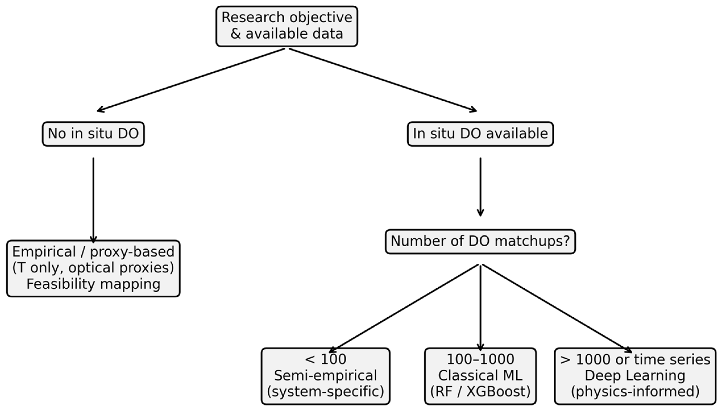
The decision flow diagram provided in Figure 3 illustrates the progression from empirical to physics-guided to data-driven approaches as the amount of data increases, or the complexity of the application increases. The final decision of the methodology will mostly depend on the availability of in situ data for DO matches, the desired level of interpretability, and the necessary temporal precision for the application. The goal of the conceptual model presented in Figure 3 is to provide a general framework that can guide the selection of a suitable approach to satellite-derived DO estimation based upon the characteristics of the application.

5.2. Comparative Results

A crucial parameter that determines the selection of the suitable dissolved oxygen retrieval method is the water body type (Table 7), with researchers reporting increased variations across water body types. Approaches established for open oceans, where optical and biogeochemical conditions are consistent, often do not directly apply to inland lakes and rivers, which exhibit more turbidity, varying depth, and pronounced spatial heterogeneity. Furthermore, unified modeling frameworks should be accompanied across various inland water bodies if local optical and biogeochemical heterogeneity is not sufficiently included. These considerations highlight the importance of balancing model generalization with environment-specific adaptation in future RS-based DO retrieval research. Figure 4 attempts to present a comparison on water bodies assessment among published studies on satellite-based dissolved oxygen concentrations. The results indicate that lakes are the most common waterbody class in the provided sheet and they also show the widest spread of method families (empirical, ML, DL, and semi-empirical). Estuaries skew toward DL here because the included estuary studies are tied to short-term forecasting.
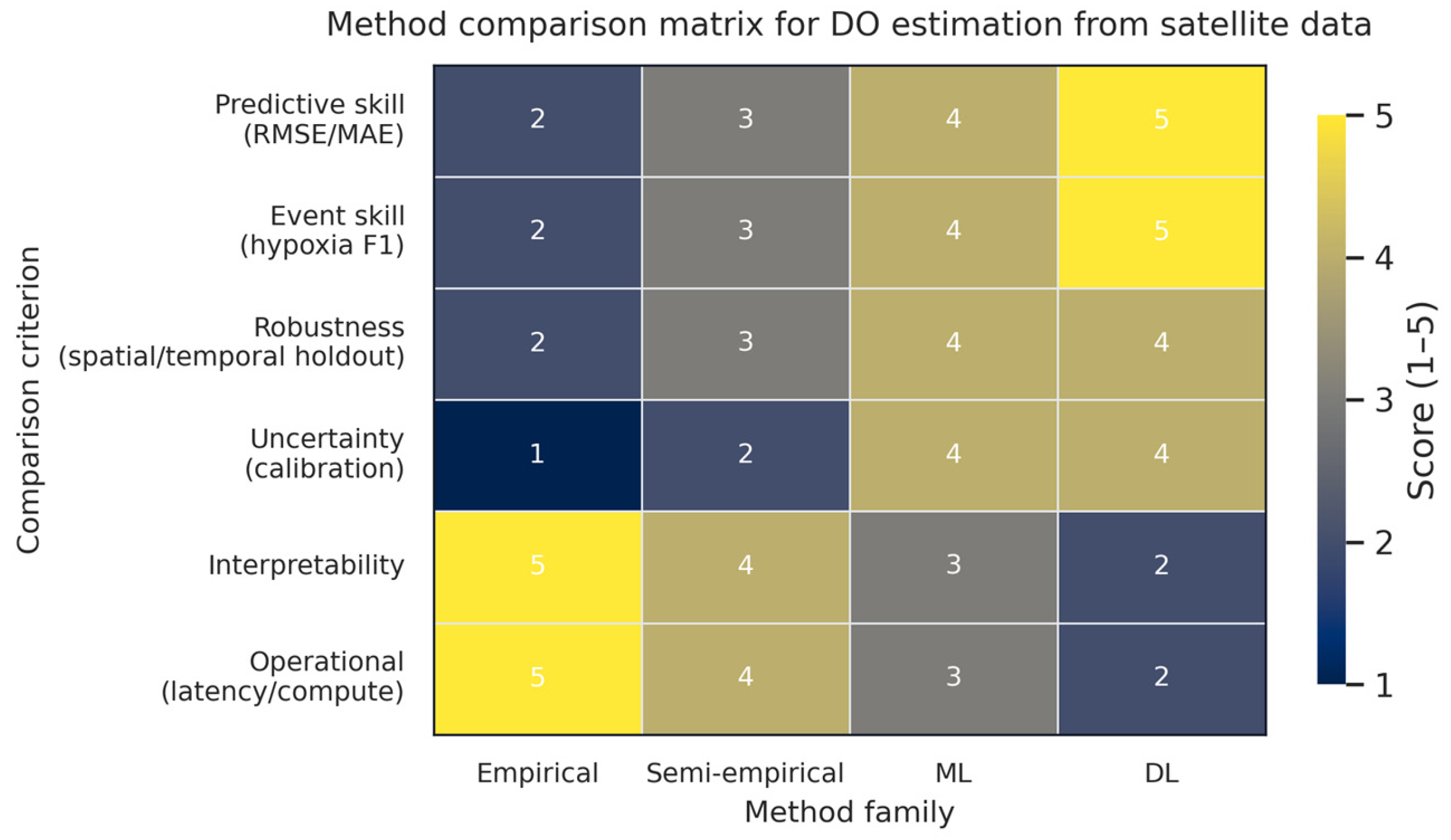
Figure 4 summarizes the comparative performance of the four dominant methodological families used for satellite-based DO retrieval using a common set of decision-relevant criteria. Rather than attempting to pool error metrics across fundamentally different study designs, waterbody types, and validation strategies, the studies revied were synthesized using a consistent rubric that reflects what the reviewed papers most frequently optimize and report. The criteria were selected to capture both model performance and practical ability to deploy in real monitoring contexts: overall predictive skill, interpretability, robustness under transfer, data requirements, event-detection capability for hypoxia, and operational feasibility.
Scoring was performed on an ordinal 1–5 scale to express relative standing across method families. These scores were assigned by triangulating repeated patterns across the included studies, emphasizing what is demonstrated under realistic evaluation settings. In particular, data requirement and operational feasibility scores reflect the end-to-end workflow burden described in the literature, including the need for in situ matchups, ancillary inputs, and computational overhead, not only the complexity of the final model form.
Across the reviewed dataset, deep learning methods occupy the upper end of the matrix for predictive skill and event skill, consistent with their frequent use in settings where nonlinear interactions and temporal context are central, such as short-term DO forecasting and hypoxia risk prediction. However, these gains co-occur with the strongest penalties in data requirement and operational feasibility. In practice, the studies that successfully deploy DL approaches typically rely on long multi-year records, dense matchup generation, and careful tuning, and they often require additional forcing variables beyond reflectance alone. As a result, DL is positioned as the most performance-oriented class, but also the most resource-intensive and least transparent without additional interpretability work.
Machine learning approaches show a similar but moderated pattern. They generally score high on predictive skill and robustness relative to purely empirical approaches, reflecting the ability of algorithms such as SVR, RF, and boosting models to capture nonlinearities and interactions while remaining easier to train and maintain than full deep architectures in many cases. At the same time, interpretability remains lower than for empirical and semi-empirical methods unless studies explicitly include feature attribution and sensitivity analyses. In the reviewed literature, ML is therefore best characterized as a strong compromise class: it often provides a meaningful accuracy gain and improved generalization potential, with a manageable increase in data and workflow complexity.
In contrast, empirical/statistical methods remain consistently favorable from a feasibility perspective. They score highest for low data burden and operational simplicity, aligning with their continued prevalence in single-scene mapping and limited-duration applications. The heatmap also shows, however, that empirical approaches are typically weakest on robustness and event skill. This mirrors a recurring result across papers: site-calibrated regressions can fit local conditions well, but performance degrades under transfer across seasons, optical regimes, or waterbodies, and threshold-based hypoxia behavior is difficult to capture with simple functional forms.
Semi-empirical approaches appear less frequently than the other categories in the assembled evidence base, but the heatmap highlights their distinct role. They tend to outperform purely empirical methods on interpretability while offering incremental improvements in robustness through constraints or process-informed structure. Their placement suggests that semi-empirical models are most useful when the application requires scientifically defensible relationships and clearer explanatory value, even if they do not always match the headline predictive skill of ML/DL in data-rich contexts.
In comparison, the heatmap supports the notion that methodological choice is best framed as a trade-off among accuracy, transferability, interpretability, and deployment constraints. The scientific literature increasingly demonstrates that ML/DL can deliver superior predictive and event skills when training data and evaluation design support generalization, but empirical and semi-empirical approaches remain competitive and often preferable when monitoring programs face limited matchup data, require transparency, or prioritize operational stability. This synthesis also underscores that reported performance is strongly coupled with validation practice; consequently, claims of superiority are most convincing when supported by spatial/temporal holdouts that explicitly test transfer beyond the calibration domain.

6. Conclusions

The recent emergence of satellite-based dissolved oxygen (DO) datasets is an important technological improvement in the measurement and evaluation of the status of aquatic ecosystems, and in the identification of the locations of hypoxia. It represents a significant enhancement in the methodology used to evaluate and manage aquatic systems through the elimination of the need for extensive field measurements at many points in space and time, which would otherwise be required using the current technologies available to measure dissolved oxygen in the environment [3]. The application of this technology will allow, for the first time, for the ability to conduct continuous, wide-scale monitoring, which is needed to assess both the impact of rapidly changing hydrodynamics and to study large geographic areas and therefore allowing critical assessment of the impact of ocean deoxygenation due to climate change [74].
Additionally, the creation of this technology has provided a valuable tool for the effective management of water resources and the protection of water bodies worldwide. Monitoring DO levels is an operational tool that provides a basis for responding to climate change in aquatic environments. Many water quality standards and ecological criteria rely on DO thresholds to evaluate environmental conditions, to establish fisheries and conservation policies, and to trigger management responses such as the release of excess water through dam releases, aeration, and reduction in nutrient loads. DO data collected with spatial and temporal resolution will allow aquatic resource managers to locate areas and time periods where recurrent hypoxia resulting from the interaction of global warming and eutrophication occurs. Therefore, early detection and response capabilities will be dependent upon the availability of DO data at the appropriate scale.
In order to validate and enhance the utility of these satellite-based DO concentration datasets, it is essential to rigorously compare their values with independently measured in situ values [75]. In addition, quantitative comparisons can be made to verify the reliability and applicability of these satellite-based DO concentration models, and numerous advanced machine learning models have demonstrated excellent predictive capabilities and performance metrics, including R2 coefficients of greater than 0.80, in aquatic environments, with some models demonstrating very high levels of accuracy, such as R2 = 0.958 for a global model [20]. This field has transitioned distinctly and necessarily from the use of empirical models to that of sophisticated machine learning (ML) and deep learning (DL) models, often in combination with other modeling approaches [2]. This transition is driven by the ability of ML/DL algorithms to fit complex, non-linear relationships between DO, an optically inactive parameter and its optically active proxies such as Chlorophyll-a and water temperature [2,76].
While ML/DL models may provide increased accuracy and robustness in managing complex, high-dimensional inputs, they also present inherent trade-offs. The advantages include the ability to provide significantly better accuracy and robustness in managing complex, high-dimensional inputs compared to traditional methods [44]. The increasing use of explainable AI (XAI) techniques, such as SHAP analysis, is providing greater transparency into how features contribute to decisions, thereby adding value to decision makers [76,77]. However, the primary disadvantages of ML/DL models relate to their dependence on large, diverse, high-quality training datasets. Therefore, the quality of the input data for these models is of paramount importance to ensure the model performs well, since errors in atmospheric corrections or difficulties associated with synchronizing satellite overpass times and intermittent field sampling times can negatively affect model performance [22,67]. Therefore, while these site-specific models may be transferable to new sites or time periods, they often require recalibration and/or parameter optimization to ensure acceptable performance. Preprocessing of satellite data, encompassing atmospheric correction and radiometric calibration, is essential for accurate DO inversion; however, specific processes related to individual sensors are not covered in this study and can be found in referenced material.
Satellite-based dissolved oxygen (DO) measurement offers several possibilities for applications in water quality management and aquatic ecosystem management. After site specific calibration of satellite-based DO concentrations, sea surface DO monitor networks will provide continuous spatial coverage of large areas of difficult-to-reach or inaccessible water bodies, thereby enabling the detection of hypoxic and anoxic zones at larger spatial scales than possible using point sampling techniques alone. This capability will likely be very useful in identifying seasonal and episodic hypoxia events that occur in lakes, reservoirs, estuaries, and coastal waters. The use of RS-estimated DO values in combination with hydrodynamic and biogeochemical models also may support the development of early warning systems for impending water quality degradations, which could allow for the implementation of proactive management and/or policy decisions prior to actual degradations. Future advancements in satellite sensor technology, retrieval algorithms, and data assimilation techniques are expected to enhance the operational application of remote sensing-based dissolved oxygen monitoring in water quality management strategies.

Author Contributions

Conceptualization: I.Z.; Investigation, I.B.; writing—original draft, I.B.; writing—review and editing, I.Z. All authors have read and agreed to the published version of the manuscript.

Funding

This research was funded by EEA and Norway Grants 2014–2021 through the project “BLUE-GREENWAY: Innovative solutions for improving the environmental status of eutrophic and anoxic coastal ecosystems” (project number 2018-1-0284, Support for Regional Cooperation).

Data Availability Statement

No new data were created or analyzed in this study. Data sharing is not applicable to this article. An OSF project was created to enhance transparency, while the review protocol was not prospectively registered nor the protocol created, which is consistent with PRISMA 2020 guidelines for non-registered reviews.

Acknowledgments

During the preparation of this manuscript/study, the authors used Grammarly, v.2.3 for the purposes of English Editing. The authors have reviewed and edited the output and take full responsibility for the content of this publication.

Conflicts of Interest

The authors declare no conflicts of interest. The funders had no role in the design of the study; in the collection, analyses, or interpretation of data; in the writing of the manuscript; or in the decision to publish the results.

Abbreviations

The following abbreviations are used in this manuscript:
BODBiochemical Oxygen Demand
CBPChesapeake Bay Program
CODChemical Oxygen Demand
CDOMColored Dissolved Organic Material
Chl-aChlorophyll-a
DLDeep Learning
DODissolved Oxygen.
DO-MDNNDissolved Oxygen Multimodal Deep Neural Network
DO-TDissolved Oxygen-Temperature
FDOMFluorescent Dissolved Organic Matter
GLODAPv2Global Ocean Data Analysis Project
KOEMKorea Marine Environment Management Corporation
LMGLindeman–Merenda–Gold
LSTMLong Short-Term Memory
MLMachine Learning
MLRMultiple Linear Regression
ML/DLMachine Learning/Deep Learning
NOAPNon-Optically Active Parameter
OACsOptically Active Constituents
OMZsOxygen Minimum Zones
RFRandom Forest
RMSERoot Mean Squared Error
RSRemote Sensing
RSRResponse Surface Regression
SMAPESymmetric Mean Absolute Percentage Error
SSTSea Surface Temperature
SPMSuspended Particulate Matter
TIRThermal Infrared
TNTotal Nitrogen
TPTotal Phosphorus
TSSTotal Suspended Solids
SVRSupport Vector Regression
WODWorld Ocean Database
XAIExplainable AI
2D-CNNTwo-Dimensional Convolutional Neural Network

References

  1. Guo, H.; Huang, J.J.; Zhu, X.; Wang, B.; Tian, S.; Xu, W.; Mai, Y. A Generalized Machine Learning Approach for Dissolved Oxygen Estimation at Multiple Spatiotemporal Scales Using Remote Sensing. Environ. Pollut. 2021, 288, 117734. [Google Scholar] [CrossRef] [PubMed]
  2. Ali, A.; Zhou, G.; Jing, G.; PabloAntezana Lopez, F.; Sun, K.; Jiang, C.; Ma, Z.; Tan, Y. XGB-2D CNN-Based Dissolved Oxygen Inversion for Coastal Water. IEEE J. Sel. Top. Appl. Earth Obs. Remote Sens. 2025, 18, 21289–21304. [Google Scholar] [CrossRef]
  3. Shi, K.; Lang, Q.; Wang, P.; Yang, W.; Chen, G.; Yin, H.; Zhang, Q.; Li, W.; Wang, H. Dissolved Oxygen Concentration Inversion Based on Himawari-8 Data and Deep Learning: A Case Study of Lake Taihu. Front. Environ. Sci. 2023, 11, 1230778. [Google Scholar] [CrossRef]
  4. Knutsen, Ø.; Stefanakos, C.; Slagstad, D.; Ellingsen, I.; Zacharias, I.; Biliani, I.; Berg, A. Studying the Evolution of Hypoxia/Anoxia in Aitoliko Lagoon, Greece, Based on Measured and Modeled Data. Front. Mar. Sci. 2024, 11, 1299202. [Google Scholar] [CrossRef]
  5. Rigaud, S.; Deflandre, B.; Grenz, C.; Cesbron, F.; Pozzato, L.; Voltz, B.; Grémare, A.; Romero-Ramirez, A.; Mirleau, P.; Meulé, S.; et al. Benthic Oxygen Dynamics and Implication for the Maintenance of Chronic Hypoxia and Ecosystem Degradation in the Berre Lagoon (France). Estuar. Coast. Shelf Sci. 2021, 258, 107437. [Google Scholar] [CrossRef]
  6. Forth, M.; Liljebladh, B.; Stigebrandt, A.; Hall, P.O.J.; Treusch, A.H. Effects of Ecological Engineered Oxygenation on the Bacterial Community Structure in an Anoxic Fjord in Western Sweden. ISME J. 2015, 9, 656–669. [Google Scholar] [CrossRef]
  7. Mondal, I.; Hossain, S.A.; Roy, S.K.; Karmakar, J.; Jose, F.; De, T.K.; Nguyen, T.T.; Elkhrachy, I.; Nguyen, N.M. Assessing Intra and Interannual Variability of Water Quality in the Sundarban Mangrove Dominated Estuarine Ecosystem Using Remote Sensing and Hybrid Machine Learning Models. J. Clean. Prod. 2024, 442, 140889. [Google Scholar] [CrossRef]
  8. Altieri, A.H.; Diaz, R.J. Dead Zones: Oxygen Depletion in Coastal Ecosystems, 2nd ed.; Elsevier Ltd.: Amsterdam, The Netherlands, 2019; ISBN 9780128050521. [Google Scholar]
  9. Ping, B.; Meng, Y.; Su, F.; Xue, C.; Li, Z.; Yuan, Z. Distribution of Surface Dissolved Oxygen Fronts in China’s Marginal Seas. J. Geophys. Res. Ocean. 2025, 130, e2025JC022789. [Google Scholar] [CrossRef]
  10. Wang, Z.; Xue, C.; Ping, B. A Reconstructing Model Based on Time–Space–Depth Partitioning for Global Ocean Dissolved Oxygen Concentration. Remote Sens. 2024, 16, 228. [Google Scholar] [CrossRef]
  11. Triana, K.; Wahyudi, A.J. Dissolved Oxygen Variability of Indonesian Seas over Decades as Detected by Satellite Remote Sensing. IOP Conf. Ser. Earth Environ. Sci. 2021, 925, 012003. [Google Scholar] [CrossRef]
  12. Peterson, K.T.; Sagan, V.; Sloan, J.J. Deep Learning-Based Water Quality Estimation and Anomaly Detection Using Landsat-8/Sentinel-2 Virtual Constellation and Cloud Computing. GISci. Remote Sens. 2020, 57, 510–525. [Google Scholar] [CrossRef]
  13. Park, S.; Lee, T.; Kim, K. High-Resolution Spatio-Temporal Monitoring of Coastal Hypoxia Using Machine Learning Models and GOCI–MODIS Satellite Data. Mar. Pollut. Bull. 2026, 222, 118871. [Google Scholar] [CrossRef]
  14. Huang, S.; Shao, J.; Chen, Y.; Qi, J.; Wu, S.; Zhang, F.; He, X.; Du, Z. Reconstruction of Dissolved Oxygen in the Indian Ocean from 1980 to 2019 Based on Machine Learning Techniques. Front. Mar. Sci. 2023, 10, 1291232. [Google Scholar] [CrossRef]
  15. Gani, M.A.; Sajib, A.M.; Siddik, M.A.; Moniruzzaman, M. Assessing the Impact of Land Use and Land Cover on River Water Quality Using Water Quality Index and Remote Sensing Techniques. Environ. Monit. Assess. 2023, 195, 449. [Google Scholar] [CrossRef] [PubMed]
  16. Singh, N.; Nalgire, S.M.; Gupta, M.; Chinnasamy, P. Potential of Open Source Remote Sensing Data for Improved Spatiotemporal Monitoring of Inland Water Quality in India: Case Study of Gujarat. Photogramm. Eng. Remote Sens. 2022, 88, 155–163. [Google Scholar] [CrossRef]
  17. Liu, M.; Wang, L.; Qiu, F. Using MODIS Data to Track the Long-Term Variations of Dissolved Oxygen in Lake Taihu. Front. Environ. Sci. 2022, 10, 1096843. [Google Scholar] [CrossRef]
  18. Salas, E.A.L.; Kumaran, S.S.; Partee, E.B.; Willis, L.P.; Mitchell, K. Potential of Mapping Dissolved Oxygen in the Little Miami River Using Sentinel-2 Images and Machine Learning Algorithms. Remote Sens. Appl. Soc. Environ. 2022, 26, 100759. [Google Scholar] [CrossRef]
  19. Yan, Y.; Wang, Y.; Yu, C.; Zhang, Z. Multispectral Remote Sensing for Estimating Water Quality Parameters: A Comparative Study of Inversion Methods Using Unmanned Aerial Vehicles (UAVs). Sustainability 2023, 15, 10298. [Google Scholar] [CrossRef]
  20. Liu, G.; Yu, X.; Zhang, J.; Wang, X.; Xu, N.; Ali, S. Reconstruction of the Three-Dimensional Dissolved Oxygen and Its Spatio-Temporal Variations in the Mediterranean Sea Using Machine Learning. J. Environ. Sci. 2025, 157, 710–728. [Google Scholar] [CrossRef]
  21. Feng, Y.; He, Y. Assessing Dissolved Oxygen Dynamics in the North Mainstream of the Dongjiang River, China Using Remote Sensing and Field Measurements. Environ. Monit. Assess. 2025, 197, 704. [Google Scholar] [CrossRef]
  22. Yang, H.; Kong, J.; Hu, H.; Du, Y.; Gao, M.; Chen, F. A Review of Remote Sensing for Water Quality Retrieval: Progress and Challenges. Remote Sens. 2022, 14, 1770. [Google Scholar] [CrossRef]
  23. Cao, J.; Wen, X.; Luo, D.; Tan, Y. Study on Water Quality Inversion Model of Dianchi Lake Based on Landsat 8 Data. J. Spectrosc. 2022, 2022, 3341713. [Google Scholar] [CrossRef]
  24. Sajib, A.M.; Uddin, M.G.; Rahman, A.; Ahmadian, R.; Olbert, A.I. Remote Sensing Applications for Monitoring Optically Inactive Water Quality Indicators: A Comprehensive Review. Earth Sci. Rev. 2025, 271, 105259. [Google Scholar] [CrossRef]
  25. Dong, L.; Wang, D.; Song, L.; Gong, F.; Chen, S.; Huang, J.; He, X. Monitoring Dissolved Oxygen Concentrations in the Coastal Waters of Zhejiang Using Landsat-8/9 Imagery. Remote Sens. 2024, 16, 1951. [Google Scholar] [CrossRef]
  26. Li, L.; Sun, B.; Xue, C.; Zheng, Z.; Ma, Y. An Enhanced Transfer Learning Remote Sensing Inversion of Coastal Water Quality: A Case Study of Dissolved Oxygen. IEEE J. Sel. Top. Appl. Earth Obs. Remote Sens. 2025, 18, 21065–21076. [Google Scholar] [CrossRef]
  27. Shao, J.; Huang, S.; Chen, Y.; Qi, J.; Wang, Y.; Wu, S.; Liu, R.; Du, Z. Satellite-Based Global Sea Surface Oxygen Mapping and Interpretation with Spatiotemporal Machine Learning. Environ. Sci. Technol. 2024, 58, 498–509. [Google Scholar] [CrossRef]
  28. Lin, S.; Pierson, D.C.; Ladwig, R.; Kraemer, B.M.; Hu, F.R.S. Multi-Model Machine Learning Approach Accurately Predicts Lake Dissolved Oxygen with Multiple Environmental Inputs. Earth Space Sci. 2024, 11, e2023EA003473. [Google Scholar] [CrossRef]
  29. Baxa, M.; Musil, M.; Kummel, M.; Hanzlík, P.; Tesařová, B.; Pechar, L. Dissolved Oxygen Deficits in a Shallow Eutrophic Aquatic Ecosystem (Fishpond)—Sediment Oxygen Demand and Water Column Respiration Alternately Drive the Oxygen Regime. Sci. Total Environ. 2021, 766, 142647. [Google Scholar] [CrossRef]
  30. Toming, K.; Liu, H.; Soomets, T.; Uuemaa, E.; Nõges, T.; Kutser, T. Estimation of the Biogeochemical and Physical Properties of Lakes Based on Remote Sensing and Artificial Intelligence Applications. Remote Sens. 2024, 16, 464. [Google Scholar] [CrossRef]
  31. Peterson, R.N.; Moore, W.S.; Chappel, S.L.; Viso, R.F.; Libes, S.M.; Peterson, L.E. A New Perspective on Coastal Hypoxia: The Role of Saline Groundwater. Mar. Chem. 2016, 179, 1–11. [Google Scholar] [CrossRef]
  32. Georgiou, N.; Fakiris, E.; Koutsikopoulos, C.; Papatheodorou, G.; Christodoulou, D.; Dimas, X.; Geraga, M.; Kapellonis, Z.G.; Vaziourakis, K.M.; Noti, A.; et al. Spatio-Seasonal Hypoxia/Anoxia Dynamics and Sill Circulation Patterns Linked to Natural Ventilation Drivers, in a Mediterranean Landlocked Embayment: Amvrakikos Gulf, Greece. Geosciences 2021, 11, 241. [Google Scholar] [CrossRef]
  33. Adjovu, G.E.; Stephen, H.; James, D.; Ahmad, S. Overview of the Application of Remote Sensing in Effective Monitoring of Water Quality Parameters. Remote Sens. 2023, 15, 1938. [Google Scholar] [CrossRef]
  34. Miao, S.; Liu, C.; Qian, B.; Miao, Q. Remote Sensing-Based Water Quality Assessment for Urban Rivers: A Study in Linyi Development Area. Environ. Sci. Pollut. Res. 2020, 27, 34586–34595. [Google Scholar] [CrossRef]
  35. Gholizadeh, M.H.; Melesse, A.M.; Reddi, L. A Comprehensive Review on Water Quality Parameters Estimation Using Remote Sensing Techniques. Sensors 2016, 16, 1298. [Google Scholar] [CrossRef] [PubMed]
  36. Ahmed, M.; Mumtaz, R.; Anwar, Z.; Shaukat, A.; Arif, O.; Shafait, F. A Multi–Step Approach for Optically Active and Inactive Water Quality Parameter Estimation Using Deep Learning and Remote Sensing. Water 2022, 14, 2112. [Google Scholar] [CrossRef]
  37. Yang, Z.; Gong, C.; Ji, T.; Hu, Y.; Li, L. Water Quality Retrieval from ZY1-02D Hyperspectral Imagery in Urban Water Bodies and Comparison with Sentinel-2. Remote Sens. 2022, 14, 5029. [Google Scholar] [CrossRef]
  38. Tian, S.; Guo, H.; Xu, W.; Zhu, X.; Wang, B.; Zeng, Q.; Mai, Y.; Huang, J.J. Remote Sensing Retrieval of Inland Water Quality Parameters Using Sentinel-2 and Multiple Machine Learning Algorithms. Environ. Sci. Pollut. Res. 2023, 30, 18617–18630. [Google Scholar] [CrossRef]
  39. Mao, K.; Wang, D.; Cai, S.; Zhou, T.; Zhang, W.; Yang, Q.; Li, Z.; Yang, X.; Picco, L. Retrieval of Dissolved Oxygen Concentrations in Fishponds in the Guangdong–Hong Kong–Macao Greater Bay Area Using Satellite Imagery and Machine Learning. Remote Sens. 2025, 17, 2277. [Google Scholar] [CrossRef]
  40. Qing, S.; Cui, T.; Lai, Q.; Bao, Y.; Diao, R.; Yue, Y.; Hao, Y. Improving Remote Sensing Retrieval of Water Clarity in Complex Coastal and Inland Waters with Modified Absorption Estimation and Optical Water Classification Using Sentinel-2 MSI. Int. J. Appl. Earth Obs. Geoinf. 2021, 102, 102377. [Google Scholar] [CrossRef]
  41. Li, Y.; Shi, K.; Zhang, Y.; Zhu, G.; Qin, B.; Zhang, Y.; Liu, M.; Zhu, M.; Dong, B.; Guo, Y. Remote Sensing of Column-Integrated Chlorophyll a in a Large Deep-Water Reservoir. J. Hydrol. 2022, 610, 127918. [Google Scholar] [CrossRef]
  42. Dash, P.; Saha, K.; Digiacomo, P.; Miller, S.D.; Zhang, H.M.; Lazzaro, R.; Son, S. Trends in Satellite-Based Ocean Parameters through Integrated Time Series Decomposition and Spectral Analysis. Part I: Chlorophyll, Sea Surface Temperature, and Sea Level Anomaly. J. Atmos. Ocean. Technol. 2025, 42, 91–123. [Google Scholar] [CrossRef]
  43. Najafzadeh, M.; Basirian, S. Evaluation of River Water Quality Index Using Remote Sensing and Artificial Intelligence Models. Remote Sens. 2023, 15, 2359. [Google Scholar] [CrossRef]
  44. Guo, H.; Zhu, X.; Jeanne Huang, J.; Zhang, Z.; Tian, S.; Chen, Y. An Enhanced Deep Learning Approach to Assessing Inland Lake Water Quality and Its Response to Climate and Anthropogenic Factors. J. Hydrol. 2023, 620, 129466. [Google Scholar] [CrossRef]
  45. Abualhin, K.; Abushaban, S. Predictive Models of Non-Optically Active Coastal Water Quality Parameters by Remote Sensing Imagery. Marit. Technol. Res. 2025, 7, 274944. [Google Scholar] [CrossRef]
  46. Dong, L.; Gong, C.; Huai, H.; Wu, E.; Lu, Z.; Hu, Y.; Li, L.; Yang, Z. Retrieval of Water Quality Parameters in Dianshan Lake Based on Sentinel-2 MSI Imagery and Machine Learning: Algorithm Evaluation and Spatiotemporal Change Research. Remote Sens. 2023, 15, 5001. [Google Scholar] [CrossRef]
  47. Al-Shaibah, B.; Liu, X.; Zhang, J.; Tong, Z.; Zhang, M.; El-Zeiny, A.; Faichia, C.; Hussain, M.; Tayyab, M. Modeling Water Quality Parameters Using Landsat Multispectral Images: A Case Study of Erlong Lake, Northeast China. Remote Sens. 2021, 13, 1603. [Google Scholar] [CrossRef]
  48. Singh, R.B.; Yurembam, G.S.; Jhajharia, D.; Kusre, B.C. Water Quality Assessment of Loktak Lake, Manipur Using Landsat 9 Imagery. Water Pract. Technol. 2024, 19, 2613–2631. [Google Scholar] [CrossRef]
  49. Ahmed, W.; Mohammed, S.; El-Shazly, A.; Morsy, S. Tigris River Water Surface Quality Monitoring Using Remote Sensing Data and GIS Techniques. Egypt. J. Remote Sens. Space Sci. 2023, 26, 816–825. [Google Scholar] [CrossRef]
  50. Zheng, Z.; Jiang, Y.; Zhang, Q.; Zhong, Y.; Wang, L. A Feature Selection Method Based on Relief Feature Ranking with Recursive Feature Elimination for the Inversion of Urban River Water Quality Parameters Using Multispectral Imagery from an Unmanned Aerial Vehicle. Water 2024, 16, 1029. [Google Scholar] [CrossRef]
  51. Kashtan Sundararaman, H.K.; Shanmugam, P. Estimates of the Global Ocean Surface Dissolved Oxygen and Macronutrients from Satellite Data. Remote Sens. Environ. 2024, 311, 114243. [Google Scholar] [CrossRef]
  52. Kim, Y.H.; Son, S.; Kim, H.C.; Kim, B.; Park, Y.G.; Nam, J.; Ryu, J. Application of Satellite Remote Sensing in Monitoring Dissolved Oxygen Variabilities: A Case Study for Coastal Waters in Korea. Environ. Int. 2020, 134, 105301. [Google Scholar] [CrossRef] [PubMed]
  53. Zhao, Z.; Huang, C.; Meng, L.; Lu, L.; Wu, Y.; Fan, R.; Li, S.; Sui, Z.; Huang, T.; Huang, C.; et al. Eutrophication and Lakes Dynamic Conditions Control the Endogenous and Terrestrial {POC} Observed by Remote Sensing: Modeling and Application. Ecol. Indic. 2021, 129, 107907. [Google Scholar] [CrossRef]
  54. Martellucci, R.; Menna, M.; Mauri, E.; Pirro, A.; Gerin, R.; Paladini de Mendoza, F.; Garić, R.; Batistić, M.; di Biagio, V.; Giordano, P.; et al. Recent Changes of the Dissolved Oxygen Distribution in the Deep Convection Cell of the Southern Adriatic Sea. J. Mar. Syst. 2024, 245, 103988. [Google Scholar] [CrossRef]
  55. Zheng, G.; Schollaert Uz, S.; St-Laurent, P.; Friedrichs, M.A.M.; Mehta, A.; DiGiacomo, P.M. Hypoxia Forecasting for Chesapeake Bay Using Artificial Intelligence. Artif. Intell. Earth Syst. 2024, 3, 230054. [Google Scholar] [CrossRef]
  56. Qi, C.; Huang, S.; Wang, X. Monitoring Water Quality Parameters of Taihu Lake Based on Remote Sensing Images and LsTM-RnN. IEEE Access 2020, 8, 188068–188081. [Google Scholar] [CrossRef]
  57. Beal, M.R.W.; Özdoğan, M.; Block, P.J. A Machine Learning and Remote Sensing-Based Model for Algae Pigment and Dissolved Oxygen Retrieval on a Small Inland Lake. Water Resour. Res. 2024, 60, e2023WR035744. [Google Scholar] [CrossRef]
  58. Tesfaye, A. Remote Sensing-Based Water Quality Parameters Retrieval Methods: A Review. East Afr. J. Environ. Nat. Resour. 2024, 7, 80–97. [Google Scholar] [CrossRef]
  59. Pizani, F.M.C.; Maillard, P.; Ferreira, A.F.F.; De Amorim, C.C. Estimation of Water Quality in a Reservoir from Sentinel-2 Msi and Landsat-8 Oli Sensors. ISPRS Ann. Photogramm. Remote Sens. Spat. Inf. Sci. 2020, 5, 401–408. [Google Scholar] [CrossRef]
  60. El Ouali, A.; El Hafyani, M.; Roubil, A.; Lahrach, A.; Essahlaoui, A.; Hamid, F.E.; Muzirafuti, A.; Paraforos, D.S.; Lanza, S.; Randazzo, G. Modeling and Spatiotemporal Mapping of Water Quality through Remote Sensing Techniques: A Case Study of the Hassan Addakhil Dam. Appl. Sci. 2021, 11, 9297. [Google Scholar] [CrossRef]
  61. Wibisana, H.; Aryaseta, B.; Wardhani, P.C. Analysis of Dissolved Oxygen on Tuban Coast Using Remote Sensing Algorithms From Landsat 8 Satellite Image Data and Interpolated Polynomials. Rev. Gest. Soc. Ambient. 2024, 18, e05321. [Google Scholar] [CrossRef]
  62. Hernández-Martínez, J.L.; Perera-Burgos, J.A.; Acosta-González, G.; Alvarado-Flores, J.; Li, Y.; Leal-Bautista, R.M. Assessment of Physicochemical Parameters by Remote Sensing of Bacalar Lagoon, Yucatán Peninsula, Mexico. Water 2024, 16, 159. [Google Scholar] [CrossRef]
  63. Cao, X.; Zhang, J.; Meng, H.; Lai, Y.; Xu, M. Remote Sensing Inversion of Water Quality Parameters in the Yellow River Delta. Ecol. Indic. 2023, 155, 110914. [Google Scholar] [CrossRef]
  64. Shi, K.; Wang, P.; Yin, H.; Lang, Q.; Wang, H.; Chen, G. Dissolved Oxygen Concentration Inversion Based on Himawari-8 Imagery and Machine Learning: A Case Study of Lake Chaohu. Water 2023, 15, 3081. [Google Scholar] [CrossRef]
  65. Theologou, I.; Patelaki, M.; Karantzalos, K. Can Single Empirical Algorithms Accurately Predict Inland Shallow Water Quality Status from High Resolution, Multi-Sensor, Multi-Temporal Satellite Data? Int. Arch. Photogramm. Remote Sens. Spat. Inf. Sci. 2015, 40, 1511–1516. [Google Scholar] [CrossRef]
  66. Cruz-Montes, E.E.; Durango-Banquett, M.M.; Torres-Bejarano, F.M.; Campo-Daza, G.A.; Padilla-Mendoza, C. Remote Sensing Application Using Landsat 8 Images for Water Quality Assessments. J. Phys. Conf. Ser. 2023, 2475, 012007. [Google Scholar] [CrossRef]
  67. Chen, L.; Liu, L.; Liu, S.; Shi, Z.; Shi, C. The Application of Remote Sensing Technology in Inland Water Quality Monitoring and Water Environment Science: Recent Progress and Perspectives. Remote Sens. 2025, 17, 667. [Google Scholar] [CrossRef]
  68. Batur, E.; Maktav, D. Assessment of Surface Water Quality by Using Satellite Images Fusion Based on PCA Method in the Lake Gala, Turkey. IEEE Trans. Geosci. Remote Sens. 2019, 57, 2983–2989. [Google Scholar] [CrossRef]
  69. Arief, M. Development of Dissolved Oxygen Concentration Extraction Model Using Landsat Data Case Study: Ringgung Coastal Waters. Int. J. Remote Sens. Earth Sci. 2017, 12, 1. [Google Scholar] [CrossRef]
  70. Abayazid, H.O.; El-Adawy, A. Assessment of a Non-Optical Water Quality Property Using Space-Based Imagery in Egyptian Coastal Lake. J. Water Resour. Prot. 2019, 11, 713–727. [Google Scholar] [CrossRef]
  71. Zhao, N.; Fan, Z.; Zhao, M. A New Approach for Estimating Dissolved Oxygen Based on a High-accuracy Surface Modeling Method. Sensors 2021, 21, 3954. [Google Scholar] [CrossRef]
  72. Jiang, G.; Loiselle, S.A.; Yang, D.; Ma, R.; Su, W.; Gao, C. Remote Estimation of Chlorophyll a Concentrations over a Wide Range of Optical Conditions Based on Water Classification from VIIRS Observations. Remote Sens. Environ. 2020, 241, 111735. [Google Scholar] [CrossRef]
  73. Sethy, D.K. Predicting Water Quality Using Ensemble Machine Learning Models and Remote Sensing Data. Int. J. Environ. Sci. 2025, 11, 166–175. [Google Scholar] [CrossRef]
  74. Levin, L.A.; Breitburg, D.L. Linking Coasts and Seas to Address Ocean Deoxygenation. Nat. Clim. Change 2015, 5, 401–403. [Google Scholar] [CrossRef]
  75. Quang, N.H.; Dinh, N.T.; Dien, N.T.; Son, L.T. Calibration of Sentinel-2 Surface Reflectance for Water Quality Modelling in Binh Dinh’s Coastal Zone of Vietnam. Sustainability 2023, 15, 1410. [Google Scholar] [CrossRef]
  76. Zhu, X.; Guo, H.; Huang, J.J.; Tian, S.; Xu, W.; Mai, Y. An Ensemble Machine Learning Model for Water Quality Estimation in Coastal Area Based on Remote Sensing Imagery. J. Environ. Manag. 2022, 323, 116187. [Google Scholar] [CrossRef]
  77. Yang, W.; Fu, B.; Li, S.; Lao, Z.; Deng, T.; He, W.; He, H.; Chen, Z. Monitoring Multi-Water Quality of Internationally Important Karst Wetland through Deep Learning, Multi-Sensor and Multi-Platform Remote Sensing Images: A Case Study of Guilin, China. Ecol. Indic. 2023, 154, 110755. [Google Scholar] [CrossRef]
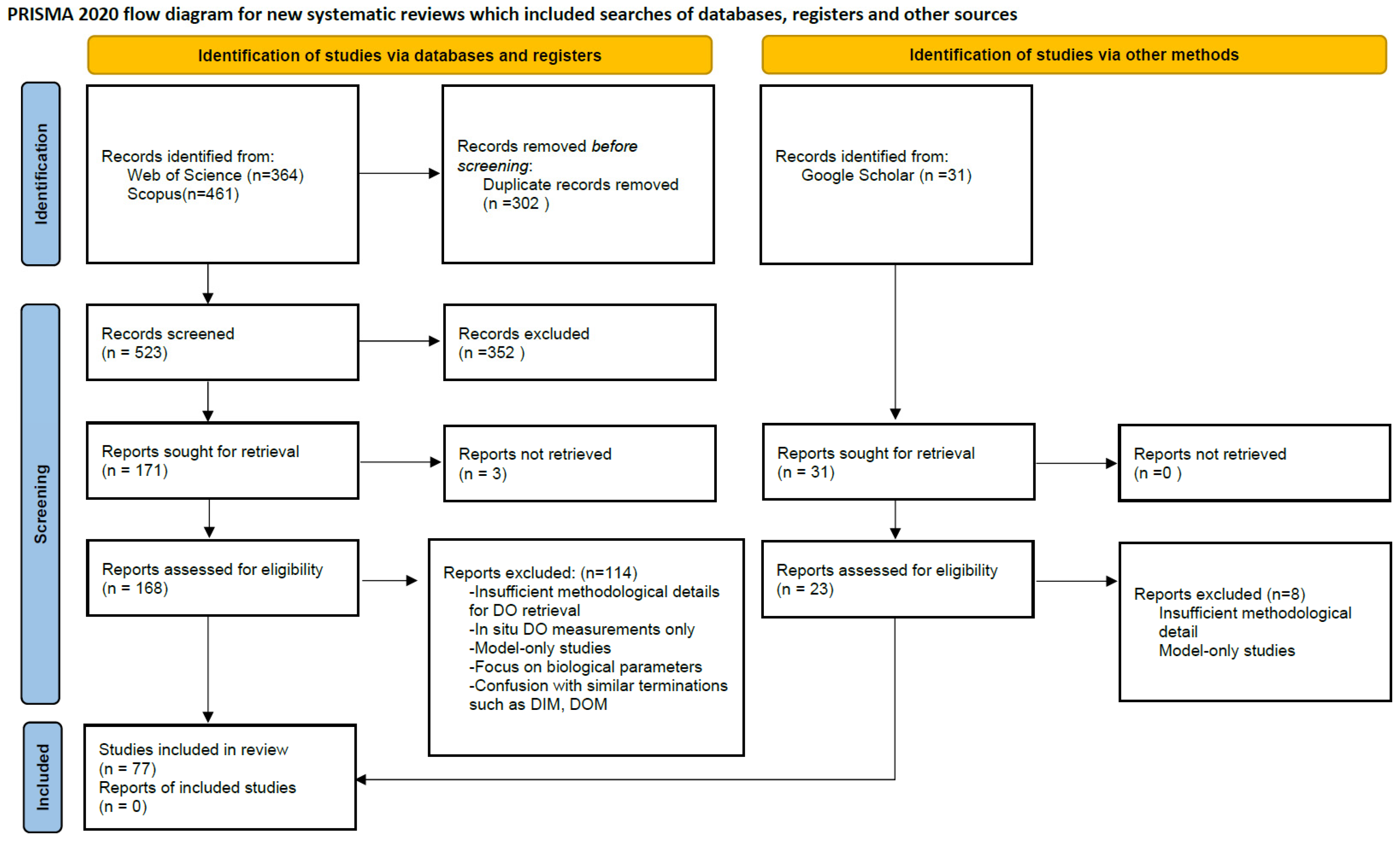
Figure 1. PRISMA 2020 flow diagram of the systematic review with the search query phrasing: “dissolved oxygen remote sensing algorithms”. Diagram visualization was prepared from the descriptions of the PRISMA online instructions (https://www.prisma-statement.org/prisma-2020-flow-diagram, accessed on 14 January 2026).
Remotesensing 18 00428 g001
Figure 2. Schematic diagram of the mechanisms that control water bodies’ dissolved oxygen.
Remotesensing 18 00428 g002
Figure 3. Conceptual model of the methodology selection to generate satellite-derived DO concentrations.
Remotesensing 18 00428 g003
Figure 4. The heatmap present the comperative evaluation of the criteria selected among the methodologies identified.
Remotesensing 18 00428 g004
Table 2. Overview of waterbody types, satellite sensors, temporal extents, and modeling methodologies that have been developed for satellite-based dissolved oxygen retrieval.
Modeling ApproachSatellite SensorsSpatial ResolutionCitation
Empirical or statisticalOcean-color/TIR, Landsat (OLI, TM, ETM+), Sentinel-2 (MSI), MODIS (Aqua/Terra/VIIRS), and Himawari-810–60 m (S2 MSI), 30 m (Landsat), 250 m–1 km (typical ocean color)[16,25,59]
Deep learningSentinel-2, Landsat (TM/ETM+/OLI) MODIS (ocean color/TIR), Himawari-810–60 m (S2 MSI), 15–30 m,
250 m–1 km (MODIS)
[3,12,14,44]
Machine learningSentinel-2 (optical); RS used together with in situ time series, Landsat (TM/ETM+/OLI), MODIS, Himawari-810–60 m (S2 MSI), 250 m–1 km (MODIS), 15–30 m[18,27]
Semi-empirical or physics-constrained/spatial-statisticalSatellite-derived reflectance + numerical model/forcing30 m (Landsat), 10–60 m (S2 MSI), 250 m–1 km (MODIS)[9,17,21]
Table 3. Summarized table determining the pros and cons of the empirical models that have been developed for satellite-based dissolved oxygen retrieval.
Main purpose
  • Quick feasibility/proof-of-concept in a single lake, reservoir, or bay.
Suitable application
  • Single system, relatively homogeneous.
  • Eutrophic/turbid or otherwise optically active waters where DO covaries strongly with Chl/TSM or temperature.
  • Focus on surface DO snapshots, not time series or forecasting.
Data requirements
  • Tens of hundreds of DO–satellite matchups.
  • Atmospherically corrected reflectance and/or TIR temperature.
Limitations
  • Highly site- and date-specific; poor generalization across years.
  • Sensors, or other water bodies, fail in oligotrophic/clear or strongly stratified systems.
  • Weak physical interpretability.
Table 4. Summarized table determining the pros and cons of the semi-empirical models that have been developed for satellite-based dissolved oxygen retrieval.
Main purpose
  • Process-aware DO mapping in one lake/region.
  • Long-term reconstructions of surface DO where stable relationships with T, clarity, Chl-a exist.
  • Attribution studies (e.g., role of warming vs. eutrophication).
Suitable application
  • Surface DO largely controlled by temperature + trophic state/light climate (e.g., shallow, well-mixed, productive systems).
  • Reasonably reliable RS products for T, Chl-a, turbidity, Secchi/Kd, pigments.
  • Interest in mechanistic interpretation, not just prediction.
Data requirements
  • Multi-season in situ DO plus co-measured T, Chl-a, clarity/turbidity
  • RS algorithms (or local calibrations) for those drivers.
Limitations
  • Inherits all biases of upstream RS products
  • Relations are system-specific; surface-only (cannot resolve deep hypoxia without extra modeling).
Table 5. Summarized table determining the pros and cons of the multivariate machine learning models that have been developed for satellite-based dissolved oxygen retrieval.
Main purpose
  • Operational regional monitoring of DO for lakes/reservoirs/coasts.
  • Seasonal–interannual trend analysis and mapping.
  • Applications need good accuracy + some interpretability (driver importance).
Suitable application
  • Medium-rich datasets: hundreds–thousands of DO–RS matchups across seasons.
  • Multiple predictors available: bands + RS-derived T, Chl, TSM, CDOM, plus static/ancillary data (depth, land use, etc.).
  • Regional domains of similar water body types (e.g., many fishponds or a lake district).
Data requirements
  • Training sets with wide coverage of DO and conditions.
  • Multi-sensor RS inputs computing for model tuning and validation.
Limitations
  • Largely region-specific.
  • Performance degrades for rare extremes (e.g., severe hypoxia) if under-sampled.
  • Needs periodic retraining if system changes (e.g., management or climate).
Table 6. Summarized table determining the pros and cons of the deep learning models that have been developed for satellite-based dissolved oxygen retrieval.
Main purpose
  • High-accuracy DO inversion in data-rich lakes/coasts.
  • Sub-daily and event-scale dynamics (using GEO data) and short-term hypoxia forecasting.
  • Large-area reconstructions where physical models are weak/expensive (regional/global DO).
Suitable application
  • Very data-rich settings: long in situ DO time series + dense satellite records (GEO or multi-sensor constellations).
  • Systems with strong non-linearities and interactions (stratification, blooms, turbidity, freshwater plumes).
  • Need to resolve time structure (diurnal cycles and rapid events) or complex spatial patterns.
Data requirements
  • Thousands–tens of thousands of labeled DO matchups; multi-modal spatiotemporal predictors.
  • GPU-class computes strong QA/QC.
Limitations
  • High complexity and expertise required.
  • Often black box (unless interpretability tools and physical constraints are added).
  • Poor cross-system transfer without retraining.
  • Vulnerable to extrapolation errors outside training envelope.
Table 7. Classification of methodologies for water bodies and sensors.
DO Retrieval Methodology ClassificationWater Body Typen StudiesCitations
Empirical or statisticalCoastal Waters3[25,45,59]
Lakes2[16,70]
Deep learningLakes3[3,12,44]
Sea1[20]
River1[12]
Machine learningRiver1[18]
Ocean1[27]
Semi-empirical or physics-constrained River1[21]
Lake1[17]
Ocean1[51]
Sea1[9]
Disclaimer/Publisher’s Note: The statements, opinions and data contained in all publications are solely those of the individual author(s) and contributor(s) and not of MDPI and/or the editor(s). MDPI and/or the editor(s) disclaim responsibility for any injury to people or property resulting from any ideas, methods, instructions or products referred to in the content.