Highlights
What are the main findings?
- A novel diffusion-guided network, FarmChanger, is proposed to overcome challenges in multi-scale structure modeling, pseudo-change suppression, and fine boundary reconstruction in farmland change detection.
- The integration of three modules—MSAD, FDFR, and GSCA—enables adaptive multi-scale feature extraction, diffusion-inspired feature refinement, and cross-feature spatial guidance, achieving superior accuracy and robustness on benchmark datasets.
What are the implications of the main findings?
- FarmChanger provides an efficient and reliable framework for large-scale and high-frequency farmland monitoring under complex seasonal and illumination variations.
- The proposed diffusion-guided and attention-enhanced mechanisms offer a transferable strategy for designing generalizable models in broader remote sensing change detection applications.
Abstract
Cultivated land is a vital resource that underpins human survival and sustainable social development. With the widespread use of high-resolution remote sensing imagery, conventional change detection methods often suffer from limited accuracy due to pseudo-changes and insufficient feature representation when dealing with complex land structures and significant seasonal variations. To address the challenges of representing multi-scale structures, mitigating pseudo-change interference, and accurately delineating boundaries in cultivated land change detection, this study proposes a diffusion-guided change detection network—FarmChanger. The network is designed based on the principles of adaptive feature extraction and diffusion-inspired feature refinement. These components are further integrated through cross-feature guidance to enhance spatial details, forming an end-to-end detection framework. Comprehensive evaluations on the CLCD and Peixian benchmark datasets demonstrate that FarmChanger achieves comparable or superior performance to mainstream models across multiple evaluation metrics, verifying its high accuracy and robustness in cultivated land dynamic monitoring tasks.
1. Introduction
Farmland serves as the fundamental resource sustaining human survival and societal development [1]. With the continuous growth of the global population and the acceleration of industrialization and urbanization, limited arable land resources are under unprecedented pressure [2,3]. Consequently, how to rapidly, accurately, and continuously obtain information on farmland changes over large areas has become a critical scientific issue of global concern.
Remote sensing technology, with its wide coverage, high timeliness, and rich information content, has become the primary approach for farmland change detection [4,5]. Early farmland change detection methods based on remote sensing imagery relied mainly on manual interpretation, identifying newly cultivated, degraded, or abandoned farmland by comparing images from two different periods [6]. These methods typically utilized medium-to-low-resolution imagery (e.g., MODIS, Landsat), which offered advantages such as low cost and broad coverage. However, the limited spatial resolution of such imagery makes it difficult to capture subtle variations in farmland, particularly in regions with complex terrain and fragmented plots. Moreover, manual interpretation requires intensive human effort, leading to long processing cycles and low efficiency, thus making it difficult to provide timely monitoring of farmland dynamics. In the context of globalization, these methods fall short of meeting the increasing demand for high-frequency, large-scale, and high-precision farmland monitoring [7].
With the advancement of high-resolution remote sensing imagery, notable advantages have been demonstrated in small-scale farmland dynamics monitoring and crop planting information extraction. However, farmland exhibits high structural complexity: different crops vary substantially in cultivation practices and growth cycles, and the presence of fallow fields further complicates the landscape. These factors collectively render change detection based on high-resolution imagery significantly more challenging.
This study proposes a diffusion-guided framework for farmland change detection, termed FarmChanger, which is designed to tackle three core challenges:
(1) Insufficient multi-scale structural representation: Farmland regions exhibit pronounced variations in spatial scale and textural structure, and existing methods struggle to achieve efficient multi-scale semantic fusion while maintaining a stable parameter budget.
(2) Feature instability induced by pseudo changes: Influenced by seasonal transitions, illumination variations, shadow effects, soil moisture conditions, and crop phenological changes, multi-temporal images contain a large amount of non-genuine change information, causing deep features to respond excessively to pseudo changes.
(3) Limited modeling capacity for fine-grained change features: Farmland change regions are often characterized by blurred boundaries and fragmented patches. Conventional decoder architectures tend to underemphasize small-scale targets and local textures, leading to inaccurate boundary localization and blurred transition regions.
To address these issues, the main contributions of this study are as follows:
Proposed a diffusion-guided farmland change detection network (FarmChanger): FarmChanger constructs an end-to-end detection framework based on “adaptive feature extraction—diffusion-based feature refinement—cross-scale change reconstruction” to enable efficient and precise identification.
Designed a Multi-Scale Adaptive Downsample Block (MSAD): This module combines multi-scale convolutional branches with attention aggregation to model complex farmland textures and scale variations, enhancing global contextual awareness while maintaining model efficiency.
Developed the Field Diffusion-inspired Feature Refiner (FDFR): Drawing on the feature guidance concept of diffusion models, this module employs conditional modulation and directional constraints to suppress pseudo-changes induced by illumination, shadows, and seasonal effects, improving robustness and semantic stability in true change discrimination.
Proposed the Guided Spatial-Cross Attention Decoder (GSCA): By synergistically leveraging spatial detail enhancement and cross-feature guidance, this module suppresses pseudo-changes, reinforces true change regions, and facilitates effective inter-layer information flow for fine-grained change representation.
Section 2 provides a detailed description of the FarmChanger network architecture and its key modules. Section 3 introduces the study area and data sources. Section 4 systematically presents the experimental design and performance evaluation of the model. Section 5 summarizes the work and discusses future research directions.
2. Method
With the advent of high-resolution remote sensing imagery, its application in fine-scale farmland dynamics monitoring and crop classification has shown unique advantages [8]. Currently, farmland change detection methods based on high-resolution imagery can be broadly categorized into two types. The first type follows a “classify-then-difference” strategy, where farmland areas are first identified in each single-period image, and the change regions are then derived through temporal differencing. Although straightforward and intuitive, the accuracy of this method heavily depends on the precision of single-period classification. Variations in image quality, acquisition conditions, and land cover characteristics often lead to unstable differencing results, with accuracy typically lower than that of single-period classification [9,10,11].
The second type is the end-to-end deep learning approach, which directly inputs multi-temporal images into a neural network to learn inter-image differences and predict change regions. Compared with the “classify-then-difference” approach, this method is more concise and efficient, and it has gradually become the mainstream direction in recent research. The performance of such methods largely depends on the network architecture, as different structures exhibit distinct advantages and limitations in feature learning and change recognition [12,13].
According to network design, existing deep learning methods can generally be divided into single-branch and multi-branch architectures. Single-branch networks typically employ a unified subnetwork to extract features and predict changes from multi-temporal images, with representative examples including the FCN and U-Net families [14,15]. For instance, Zhang et al. [16] proposed a model combining a Feature Pyramid Network (FPN) with a trapezoidal U-Net (FACNN) for ultra-high-resolution urban land-use change detection, which effectively captures multi-scale features. However, traditional U-Net architectures face a trade-off between contextual understanding and spatial localization, limiting their adaptability to complex scenes. To address this, U-Net++ [17] introduces nested skip connections and intermediate convolutional blocks to reduce the semantic gap between encoder and decoder paths. Building on this, Peng et al. [18] proposed an improved model incorporating multi-side output strategies to better exploit both global and fine-grained information, thereby mitigating error propagation. Nevertheless, while performance improved, model complexity and computational cost also increased substantially.
To address this issue, researchers have proposed dual-branch networks tailored for change detection tasks, which can be further categorized into Siamese and pseudo-Siamese networks [19]. The key distinction between them lies in whether the two branches share weights during feature extraction. In pseudo-Siamese networks, the two branches do not share weights. This architecture can effectively perform standard change detection tasks; for example, Touati et al. [20], Xu et al. [21], and Farhadi [22] all employed pseudo-Siamese networks for change detection. However, this approach primarily relies on comparing the similarity between the features extracted by the two branches, making it highly dependent on the quality of input data and the effectiveness of feature representation. Low-quality input or insufficiently discriminative features can lead to degraded classification performance and failure to achieve expected results.
In contrast, Siamese networks share parameters between the two branches, allowing the model to align and represent multi-temporal images within a consistent feature space. This enables more effective capture of change information while reducing interference from redundant features. Such architectures demonstrate strong robustness in change detection, particularly when handling imbalanced distributions of changed and unchanged pixels and have therefore become mainstream methods in the field. For instance, Yang et al. [23] employed a Siamese network for pixel-level change detection of optical aerial imagery; Jiang et al. [24] modeled complex relationships between building changes and displacements using a Siamese network; and Wang et al. [25] proposed a Siamese convolutional neural network for multi-sensor change detection. Although Siamese architectures can enhance the abstract representation of image differences and maintain relatively stable detection performance under noise, they remain prone to misclassification in scenarios with complex object boundaries or high inter-class neighborhood variability, introducing additional noise. This limitation indicates that Siamese networks still struggle with capturing long-range dependencies and global contextual information, necessitating stronger global modeling mechanisms.
Compared with existing approaches, this study conducts targeted structural designs for key modules at the architectural level. The Multi-Scale Adaptive Downsampling (MSAD) encoder is not a simple aggregation of multi-branch convolutions and attention modules; instead, it structurally decouples multi-scale convolutions from attention and performs selective recalibration only on local channel subspaces, thereby enhancing scale adaptivity while maintaining low computational overhead.
Although the Field Diffusion-inspired Feature Refiner (FDFR) is motivated by the denoising principle of diffusion models, it does not construct explicit noise injection or a reverse sampling chain. Its time steps are adaptively generated from feature statistics and are employed solely as an auxiliary discriminative branch for training supervision, rather than being directly involved in the final prediction pathway.
The Guided Spatial-Cross Attention (GSCA) differs fundamentally from conventional guided attention mechanisms. It approximates global spatial modeling via depthwise separable convolutions, constraining the computational complexity from quadratic growth to near-linear scaling. Furthermore, through a cross-feature conditional modulation mechanism, GSCA explicitly suppresses responses to pseudo changes, thereby better accommodating the practical requirements of high-resolution remote sensing change detection.
The network architecture of FarmChanger is illustrated in Figure 1, with example data derived from the CLCD dataset. FarmChanger is a deep model designed for high-resolution remote sensing cropland change detection. The overall workflow follows a dual-branch contrastive encoding, conditional feature refinement, cross-feature attention fusion, and decoding pipeline. It is designed to balance the preservation of local details with global semantic consistency under limited sample conditions, illumination variations and seasonal crop variations.
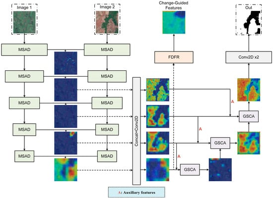
Figure 1.
Network architecture of FarmChanger. (Solid and dashed arrows indicate the main forward propagation of feature representations. The colored maps are attention heatmaps, where warmer colors (e.g., red) represent regions receiving higher attention, and cooler colors (e.g., blue) indicate less relevant areas.)
Specifically, two temporal remote sensing images (Image1 and Image2) are first processed by the MSAD encoder to extract hierarchical semantic features. At each scale, features are aligned and fused through concatenation and a convolution (Concat + Conv2D). The fused features then pass through the FDFR module to generate change-guided features for auxiliary supervision. In the decoding stage, the network employs multi-level GSCA modules to enhance spatial details and provide conditional guidance, gradually restoring the features to the original resolution. Finally, two convolution layers output the change mask. This design ensures computational efficiency while improving sensitivity to subtle and sparse changes.
In the following, the MSAD, FDFR, and GSCA modules are introduced sequentially.
2.1. Multi-Scale Adaptive Downsample (MSAD) Block
In recent years, Transformers have demonstrated distinctive advantages in modeling long-range dependencies and have been increasingly applied to change detection in remote sensing imagery. For example, Yan and Cao et al. [26] integrated the Transformer into a change detection framework, extracting multi-scale features from multi-temporal images through a hierarchical structure and combining them with a nested U-Net decoder to obtain precise change regions, while employing a simple yet effective model fusion strategy to improve detection accuracy. On large-scale public datasets such as LEVIR-CD and SYSU-CD, this approach outperformed traditional convolutional models. Yan and Wan et al. [27] proposed the Fully Transformer Network (FTN), which further models features from a global perspective and employs a pyramidal multi-level feature fusion strategy to enhance the recognition of complete change regions, achieving significant improvements across multiple public datasets.
However, networks designed based on these Transformer-based methods are often highly complex, with large parameter counts, and require substantial amounts of high-quality labeled data and computational resources. Moreover, most networks designed on mainstream change detection datasets exhibit limited recognition capability for farmland change detection [28]. Due to seasonal variations, farmland change detection datasets are often small-sample datasets, making it difficult for high-parameter Transformer-based deep learning models to achieve satisfactory performance [29,30].
Building on this, most recent studies, inspired by the Transformer paradigm, have attempted to integrate global attention mechanisms with lightweight architectures to balance global modeling capability, local feature representation, and computational efficiency. Studies [31,32] have explored combining channel-wise and global attention mechanisms with CNN or Transformer frameworks to enhance feature selection along both spatial and channel dimensions. These methods exhibit a strong feature encoding ability in small-sample, high-complexity scenarios. However, cropland change detection is characterized by significant spatial scale variation, pronounced seasonal differences, easily confusable shadows and crop textures, and limited annotated samples. Therefore, the encoder must preserve rich local details (e.g., small fields, irrigation channels, shadows, water bodies) while obtaining sufficient semantic receptive fields to capture cross-region contextual information and support stable temporal discrimination.
To balance model performance and efficiency, inspired by studies [33,34,35], we propose a lightweight yet expressive encoder module—MS-Adaptive Downsample (MSAD) Block, as illustrated in Figure 2. This module discards conventional VGG backbones with limited receptive fields and avoids computationally expensive large Transformer structures. At each downsampling stage, it incorporates hybrid multi-scale convolutional branches and lightweight attention aggregation to enhance semantic representation and suppress shadow and background interference in cropland regions, while maintaining low computational complexity.
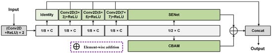
Figure 2.
Structure of the MSAD module.
When attention modules are repeatedly applied within same-scale or cross-scale architectures, their effects are not a simple linear superposition. Instead, they progressively calibrate feature responses, enabling continuous refinement of semantic representations through successive recalibration. The first attention layer primarily performs coarse-grained saliency recalibration, while subsequent attention layers further focus on local discrepancies and hard-to-distinguish regions, achieving iterative optimization of feature representations and guiding network features to gradually converge toward a more optimal semantic distribution.
In addition, multi-scale convolutional branches decompose features according to different receptive fields, allowing the model to perform representation learning at three distinct levels. This design mitigates the issues of excessive feature smoothing or attention bias that may arise from single-scale convolutions.
The processing flow of the module is as follows: First, standard small-kernel convolutions construct stable local feature representations. Parallel multi-scale convolutions then capture features at different receptive fields to complement scale variation information. Subsequently, channel and spatial attention mechanisms weight key channels and locations. The resulting features are finally fused and propagated to the subsequent stage. This design enhances the recognition of fine-scale objects (by preserving boundary integrity via small-scale convolutions), suppresses shadows and background interference (via attention mechanisms), and strengthens cross-region context modeling (via multi-scale feature fusion).
Formally, let the input feature tensor be , where is the batch size, is the number of input channels, and , denote spatial dimensions.
Convolution and downsampling: The module first applies two convolution layers with ReLU activation to obtain intermediate features, followed by downsampling:
where and denotes output channels.
Multi-branch multi-scale structure: The downsampled feature is split along the channel dimension into five sub-branches:
where , . The first three branches employ convolution kernels with different receptive fields to capture multi-scale local features: , , . The fourth branch is an identity mapping: . ()
Attention-enhanced branch: The fifth branch integrates channel attention (SE) and spatial attention (CBAM) in parallel:
Squeeze-and-Excitation (SE):
where , and is the channel reduction ratio.
CBAM: Channel-wise and spatial attention are sequentially computed to enhance key features.
Dual attention fusion:
Finally, the five branch outputs are concatenated along the channel dimension:
However, in farmland change detection tasks, high-level semantic features are highly susceptible to the combined effects of illumination conditions, shadow artifacts, variations in soil moisture, and differences in crop phenology. These factors tend to induce a large number of pseudo-difference responses in the feature space that closely resemble genuine changes. Consequently, relying solely on global attention mechanisms and multi-scale strategies is insufficient to fundamentally resolve the pseudo-difference problem.
It should be emphasized that in public change detection datasets dominated by man-made objects such as buildings and roads, the boundaries are well defined and the structures are relatively stable. As a result, their spectral and textural characteristics are less affected by the aforementioned factors, and the interference caused by pseudo differences is limited. This explains why many existing methods can still achieve high accuracy on such datasets even when the impact of pseudo differences is largely ignored [35,36,37,38,39].
2.2. Field Diffusion-Inspired Feature Refiner (FDFR) Module
In recent years, diffusion models have shown remarkable potential in generative modeling and feature optimization [40]. Their core principle is to gradually approximate the target distribution from a noise distribution through forward noising and reverse denoising processes. This progressive feature reconstruction mechanism endows the model with strong robustness to noise and the ability to reconstruct structural boundaries, enabling fine-grained feature recovery in complex backgrounds. Inspired by these characteristics, diffusion models have been applied to semantic segmentation tasks. For instance, MedSegDiff [41,42] achieves high-precision segmentation in medical images through conditional diffusion; Diff-UNet [43] integrates diffusion generation with a U-Net structure to enhance target recognition in complex scenes; and models such as SegDiff [44] and DDPM-Seg [45] employ multi-stage reconstruction of detailed features via diffusion processes.
However, farmland change detection datasets are often small, high-level features are strongly affected by seasonal variation, and boundary textures are fragmented with subtle inter-class differences [28,46]. In such tasks, employing a full diffusion process—including forward noising and iterative reverse denoising—substantially increases parameter count and computational load, while the noise injection process can weaken the representation of actual change regions, hindering network convergence and generalization. Thus, directly applying full-process diffusion models is not suitable for end-to-end farmland change segmentation tasks [47,48].
Within diffusion models, the Diffusion Guidance Head plays a central role in feature optimization by providing directional constraints and semantic guidance. Through conditional modulation or time embedding mechanisms, it discriminatively guides the reverse denoising process, enabling the model to emphasize structural boundaries and semantic consistency during feature reconstruction [44,45]. This property allows diffusion guidance heads not only to “generate” features but also to suppress noise and pseudo-changes in discriminative tasks. Consequently, they can conditionally constrain and refine deep-level generated change maps, maintaining relatively accurate representation and discrimination of true change regions even under complex background interference.
Based on this observation, this study proposes a discriminative, conditionally denoising feature refinement module (FDFR) designed to generate auxiliary supervision signals. The module simulates a diffusion-inspired “denoising–refinement” process within a discriminative framework, as illustrated in Figure 3. It treats the input feature as a “noise-contaminated representation,” models pseudo-change intensity via temporal embedding, and constrains the denoising direction through conditional modulation. The multi-scale U-Net structure enables progressive feature refinement, producing a change-guided feature that assists in loss computation without directly participating in final change prediction. During training, the loss derived from this change-guided feature serves as an auxiliary supervision signal, compelling the encoder to focus on genuine change regions, differentiate between varying change intensities, and reduce model sensitivity to pseudo-changes caused by shadows or seasonal crop variations.
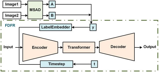
Figure 3.
Structural diagram of the FDFR module. (It should be emphasized that the MSAD module shown in the figure is provided for illustrative purposes only. It is taken from the first layer of the network and is not included in the FDFR module).
Unlike generative diffusion models, FDFR does not explicitly construct a noise-injection chain, perform noise alignment, or adopt score matching. The time step acts as a data-driven control variable rather than an iterative sampling index. The entire module is trained end-to-end under task supervision, producing refined features in a single forward pass.
The processing flow of FDFR can be divided into four stages:
(1) Conditional Generation and Embedding:
This stage generates conditional vectors as global control signals to characterize pseudo-change intensity and contextual constraints for subsequent denoising and refinement. Let the input feature of FDFR be (where B is batch size, C is channel number, and H, W are height and width). It should be noted that this conditional signal does not correspond to any physical time variable or explicit noise modeling.
Time-step generation: The global mean feature intensity for each sample is computed as:
Here, characterizes the overall response level of a sample in the feature space, rather than directly representing noise intensity in a physical sense. Considering that in SAR change detection, low-response regions (e.g., weak-scattering areas or regions with blurred boundaries) are typically associated with higher uncertainty, is adopted as an approximate statistical indicator of uncertainty magnitude.
The value is then mapped and discretized into an integer interval with :
This pseudo-temporal index is used solely to modulate the degree of feature refinement for different samples within the FDFR module. Its role is analogous to the step index in diffusion models that controls processing stages, but it does not correspond to any actual diffusion process or noise injection mechanism.
Label generation: The average difference between shallow features of the two temporal phases in the network is
This low-level difference captures fine boundary and texture variations. The continuous differences are discretized into three classes:
These pseudo-labels guide the network to distinguish pseudo-change intensities. Thus, (continuous condition) captures global pseudo-change strength, while (discrete condition) introduces local categorical constraints, jointly guiding FDFR refinement.
Conditional Embedding: Time-step embedding uses sinusoidal mapping:
where . The embedding is projected via MLP:
and label embeddings are obtained as
Finally, the condition vector is obtained as
(2) Encoding Stage (U-Net Encoder): The encoder performs layer-wise feature extraction, modulated by the condition vector , with global dependency modeling at the deepest layer.
First encoding block:
where inside each UNetBlock:
Subsequent encoding and downsampling operations follow similarly:
where .
The Transformer Fusion Module reshapes and processes through multi-head attention:
(3) Decoding Stage (U-Net Decoder): The decoder progressively restores spatial resolution using skip connections:
(4) Output Stage: The refined feature map is generated via an output convolution: .
However, the resulting change features primarily capture high-level semantic differences, while their ability to characterize boundary textures and fine-grained variations in the decoding stage remains limited.
2.3. Guided Spatial-Cross Attention (GSCA) Module
In cropland change detection, the process of progressively restoring the semantic features extracted by the encoder into a prediction mask at the same scale as the input image poses greater challenges than conventional building or road change detection tasks. These challenges include ensuring temporal consistency, distinguishing sparse and subtle changes, and suppressing pseudo-changes caused by background interference such as shadows, water bodies, clouds, or seasonal crops. Typically, cropland changes manifest as small-scale, low-contrast, fine-grained regions that are easily obscured by complex background noise. Meanwhile, during decoding, the high-resolution feature maps must recover spatial details at the pixel level. However, applying a global non-local attention mechanism directly results in quadratic computational complexity with respect to the number of pixels, imposing heavy computational and memory burdens. Furthermore, the task requires efficient multi-scale fusion between deep semantic and shallow boundary features. Simple concatenation of features often introduces redundancy and false detections. Additionally, illumination variations, seasonal transitions, and noise can induce pseudo-changes, weakening the model’s sensitivity to real changes.
To address these issues, inspired by previous studies [49,50] and the FDFR module, this study proposes a Guided Spatial-Cross Attention (GSCA) module, as illustrated in Figure 4. The GSCA consists of two components: a lightweight spatial attention submodule and a cross-feature conditional attention submodule. The spatial attention component enhances spatial detail representation through depthwise separable convolutions, while the cross-feature conditional attention component suppresses pseudo-changes and strengthens genuine change regions through guided modulation.
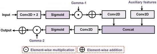
Figure 4.
Structural diagram of the GSCA module.
(1) Classical Spatial Self-Attention
Conventional spatial self-attention (non-local attention) computes pairwise similarity across all spatial positions to capture long-range dependencies. Given input features (where is batch size, the channel number, and , the spatial dimensions), and , the computation can be described as follows:
Projection:
where .
Similarity and Aggregation:
The computational complexity (ignoring batch dimension) is approximately which increases quadratically with spatial resolution. Consequently, training and inference become computationally expensive, and global aggregation often weakens local boundary and subtle variation information, making it difficult to suppress pseudo-changes from illumination or seasonal effects.
To overcome these limitations, the GSCA replaces global quadratic attention with a Local Convolution Approximation (LCA) module and a Cross-feature Conditional Guided Attention (CGA) mechanism. This two-step design reduces complexity to linear with respect to pixel count while preserving local spatial structure modeling and cross-feature conditioning capabilities.
(2) Local Convolution Approximation (LCA)
As shown in Figure 5, cropland changes typically exhibit low contrast, sparse distribution, and fine boundaries that can be easily disturbed by water, shadows, or seasonal crops. The LCA module enhances spatial responses with linear complexity during decoding, focusing on potential change regions while suppressing background noise.
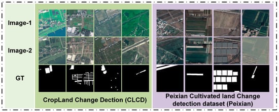
Figure 5.
Examples from the CLCD and Peixian change detection datasets. (White regions indicate areas where changes have occurred, while black regions represent unchanged areas.)
Given the main feature , the LCA process is formulated as:
where denotes a depthwise convolution with kernel size k to preserve local spatial structure, is a pointwise convolution for channel fusion, is the sigmoid function, denotes batch normalization, and is a learnable residual coefficient initialized to 0. The operator indicates element-wise multiplication.
(3) Cross-Feature Conditional Guided Attention (CGA)
Although LCA enhances local spatial features and improves sensitivity to fine-grained boundaries and textures, it cannot differentiate real changes from pseudo-changes caused by illumination, seasonal variations, or background noise. To address this limitation, we propose a Cross-feature Conditional Guided Attention (CGA) mechanism that uses auxiliary features (from skip connections) to modulate the main feature adaptively. This guided conditioning suppresses pseudo-changes while emphasizing real change regions. Unlike LCA, which enhances a single feature map locally, CGA achieves pixel-wise conditional enhancement through localized channel interactions, maintaining spatial sensitivity and complementing LCA’s deficiency in pseudo-change suppression.
Given the main feature and conditional feature , the CGA process is defined as follows:
Channel Reduction (1 × 1 Convolution):
where , and typically ranges from 4 to 8.
Local Conditional Fusion:
Conditional Attention Mask Generation:
Conditional Modulation and Residual Fusion:
where is a learnable residual coefficient initialized to 0.
Finally, the output of the GSCA module is defined as:
3. Datasets
CropLand Change Detection (CLCD) Dataset [28]:
The CLCD dataset consists of 600 pairs of cropland change samples, divided into 360, 120, and 120 pairs for training, validation, and testing, respectively. Each sample pair contains two 512 × 512 dual-temporal images and a corresponding binary change label. The images were captured by the Gaofen-2 (GF2) satellite over Guangdong Province, China, in 2017 and 2019, with a spatial resolution ranging from 0.5 to 2 m.
Peixian Cultivated Land Change Detection Dataset (Peixian) [46]:
The Peixian dataset contains 5170 pairs of 256 × 256 pixel GF2 pan-sharpened images collected from Peixian County, Jiangsu Province. The original dual-temporal images have a spatial resolution of 1 m. The dataset is divided into training, validation, and testing subsets at a ratio of 3:1:1. Data augmentation is performed through random flipping and rotation to construct a cropland change detection dataset representing the years 2018 and 2021.
Examples of cropland change samples from the CLCD and Peixian datasets are shown in Figure 5.
4. Experiments
4.1. Experimental Platform and Evaluation Metrics
All experiments were conducted on a workstation equipped with a 12th Gen Intel(R) Core(TM) i5-12490F processor, an NVIDIA GeForce RTX 4060 Ti GPU (16 GB VRAM), and 64 GB of system memory. The implementation was based on the PyTorch 1.10.2 deep learning framework, accelerated by CUDA 11.1 and cuDNN 8.1 libraries to ensure efficient training and inference.
To comprehensively evaluate the classification and segmentation performance of the proposed model in cropland change detection, six commonly used accuracy metrics were adopted: F1-score, Precision, Recall, Overall Accuracy (OA), Kappa coefficient, and Intersection over Union (IoU). These metrics are derived from the confusion matrix, where TP (True Positive) denotes the number of correctly predicted changed pixels, FP (False Positive) represents unchanged pixels incorrectly predicted as changed, FN (False Negative) corresponds to changed pixels misclassified as unchanged, and TN (True Negative) refers to pixels correctly identified as unchanged. The definitions and implications of each metric are as follows:
Precision (Pre.): Precision measures the accuracy of the model’s positive predictions and is defined as: . In cropland change detection, Precision reflects the proportion of correctly identified changed pixels among all pixels predicted as changed.
Recall (Rec.): Recall assesses the model’s ability to capture all true change regions and is defined as: . A higher Recall indicates that the model effectively detects most actual cropland changes.
F1-score (F1): F1-score balances Precision and Recall and is defined as: .
Overall Accuracy (OA): OA quantifies the overall classification correctness and is defined as: . In this context, OA represents the proportion of correctly classified pixels across the entire image, indicating the overall discriminative ability of the model.
Kappa Coefficient (Kap.): The Kappa coefficient accounts for the agreement between predicted and true labels beyond random chance and is calculated as: . where denotes the expected agreement under random classification. The Kappa coefficient ranges from −1 to 1, with higher values indicating stronger consistency between predictions and ground truth (presented as a percentage in this study).
Intersection over Union (IoU): IoU evaluates the spatial overlap between the predicted and actual change regions and is defined as: . In cropland change detection, IoU measures the spatial consistency between predicted and true change areas, serving as a key indicator of segmentation boundary accuracy.
For computational efficiency analysis, Parameters (Par., M) and Floating Point Operations (FLOPs, G) are used to quantify the model’s structural complexity and computational cost.
In this study, AdamW is adopted as the optimizer with a weight decay of 0.0025 and an initial learning rate of . The learning rate is scheduled using the CosineAnnealingWarmRestarts strategy. The loss function is the commonly used BCEWithLogitsLoss for binary classification. During evaluation, the network outputs are transformed into probabilities via a sigmoid function and binarized using a fixed threshold of 0.5, which is applied for metric computation during training and for performance evaluation in the validation stage. No form of data augmentation is employed in the entire experimental setup; all models are trained and tested on the original CLCD and Peixian datasets.
The number of training epochs is uniformly set to 100. This choice is based on a joint consideration of prediction-set performance convergence and computational efficiency. As illustrated in Figure 6, we conducted a total of 300 training epochs on the CLCD dataset, computing performance metrics on the prediction set every five epochs. The results indicate that all evaluation metrics gradually reach a stable plateau after approximately 70–80 epochs. Although certain metrics exhibit local optima at later epochs (e.g., around epoch 180), the performance gain compared with epoch 100 is less than 1–2%, while the training cost increases substantially. Balancing performance stability and computational efficiency, epoch 100 is therefore selected as the final model configuration.
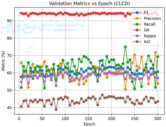
Figure 6.
Performance curves of the FarmChanger model across different training epochs.
Confidence interval estimation: To quantify the statistical uncertainty of micro-averaged metrics, a non-parametric bootstrap method based on sample-level confusion counts is employed in the comparative experiments (Section 4.3). Specifically, for each image in the test set, pixel-level confusion counts (TP, FP, TN, FN) are first computed. In each bootstrap resampling iteration (sampling with replacement, drawing N indices from N samples, repeated B = 1000 times), the confusion counts of the selected images are summed to form an aggregated confusion matrix, from which evaluation metrics such as Precision, Recall, F1-score, IoU, OA, and Kappa are calculated. Based on the empirical distributions of these metrics obtained from the B resamples, the 2.5th and 97.5th percentiles are taken to construct the 95% confidence intervals.
4.2. Ablation Study
To evaluate the effectiveness of each proposed module in cropland change detection, ablation experiments were conducted on two representative datasets—CLCD and Peixian—to assess the model’s stability and generalization capability under different terrain and imaging conditions. The ablation study focused on three key modules: FDFR, GSCA, and MSAD. For fair comparison, VGG was used as the baseline backbone network, and experiments were performed by either replacing or integrating these modules under identical hyperparameter settings (epoch = 100, batch size = 8, initial learning rate = 5 × 10⁻⁴) and training data. The quantitative results are summarized in Table 1 and Table 2, and the visual results are shown in Figure 7 and Figure 8.

Table 1.
Presents the quantitative evaluation results of the ablation study on the CLCD dataset (red bold numbers indicate the best performance for each metric, and purple bold numbers indicate the second best. The symbol “√” denotes that the corresponding module has been added.).
Table 2.
Presents the quantitative results of the ablation experiments on the Peixian dataset (red bold numbers indicate the highest values for each metric, and purple bold numbers indicate the second-best. The symbol “√” denotes that the corresponding module has been added.).
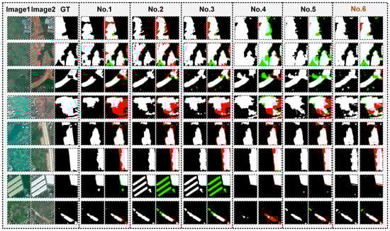
Figure 7.
Ablation study results on the CLCD dataset (green areas indicate misclassified regions, and red areas indicate undetected regions. The brown text indicates the proposed model in this work).
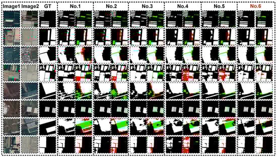
Figure 8.
Visual comparison of ablation experiments on the Peixian dataset (green areas indicate misclassified regions, and red areas indicate undetected regions) The brown text indicates the proposed model in this work.
(1) CropLand Change Detection (CLCD) Dataset
As shown in Table 1, the baseline model (No.1), which only employs the VGG backbone, achieves an F1-score of 57.20%, Precision of 66.84%, and Recall of 50.00%, indicating relatively low overall accuracy. This suggests that the baseline network struggles to accurately identify cropland change regions in complex backgrounds, being easily affected by shadows, bare soil, and phenological variations in crops.
After integrating the FDFR module into the VGG backbone (No.2), the F1-score slightly increases to 56.65%, demonstrating that the diffusion-based feature refinement mechanism improves global dependency modeling to some extent. However, the performance gain remains limited due to insufficient integration of spatial hierarchical features.
When the GSCA module is further introduced (No.3), the F1-score rises to 57.73%, and IoU improves to 40.58%, showing that the spatial cross-attention mechanism enhances the delineation of change region details. Nevertheless, under the constraint of a single-feature extraction backbone (VGG), the overall improvement remains modest.
Replacing the backbone with the MSAD architecture (No.4) leads to a significant performance boost, with the F1-score increasing to 60.02%, representing a 2.82 percentage point improvement over the baseline. This confirms the effectiveness of the multi-scale adaptive decoding structure in enhancing boundary continuity and suppressing pseudo-changes.
When FDFR is combined with MSAD (No.5), the F1-score further rises to 60.96%, with Precision and Recall becoming more balanced and the Kappa coefficient improving to 58.07%. This demonstrates that integrating refined features with global modeling enhances model stability and robustness.
Finally, when FDFR, GSCA, and MSAD are jointly employed (No.6), the model achieves optimal performance: an F1-score of 63.24%, Recall of 63.12%, Kappa coefficient of 60.29%, and IoU of 46.25%, representing an overall improvement of approximately 6 percentage points compared to the baseline. Although the parameter count slightly increases to 29.70 M, the FLOPs are only 49% of those of the VGG-based model, demonstrating an excellent balance between accuracy and computational efficiency.
(2) Peixian-Cultivated-Land-Change-Detection (Peixian) Dataset
As shown in Table 2, the baseline model (No.1, VGG backbone) already demonstrates relatively strong baseline performance (F1 = 77.92%). However, it still exhibits significant omission and false-alarm issues. After introducing the FDFR module (No.2), the F1-score improves from 77.92% to 78.68%, with simultaneous increases in Precision and Recall. This indicates that FDFR effectively mitigates pseudo-changes caused by illumination, shadow, and phenological differences in crops, leading to cleaner predictions and a noticeable reduction in false alarms (green misclassifications).
When the GSCA module is further integrated (No.3), the F1-score remains comparable (78.53%), but Precision and Recall become more balanced, suggesting that the cross-spatial attention mechanism enhances the semantic consistency of detected changes. However, under the limitation of a single VGG backbone, its performance gain remains modest.
Replacing the backbone with the MSAD architecture (No.4) results in a substantial performance improvement, with the F1-score reaching 84.57%, an increase of 6.65 percentage points over the baseline. This improvement highlights MSAD’s ability to capture continuous boundaries and fine-grained texture information through multi-scale feature fusion and adaptive decoding, significantly enhancing positional accuracy and overall stability.
Building upon MSAD, adding the FDFR module (No.5) further elevates performance, achieving an F1-score of 85.44% and Recall of 85.81%, indicating that diffusion-based feature refinement strengthens the model’s capacity to detect real change regions and reduces omission errors caused by surface inconsistencies.
Finally, when FDFR, GSCA, and MSAD are jointly employed (No.6), the model achieves its best overall performance on the Peixian dataset: F1 = 88.87%, Precision = 88.70%, Recall = 89.04%, OA = 97.12%, Kappa = 87.21%, and IoU = 79.97%. Compared with the baseline, the F1-score improves by 10.95 percentage points, demonstrating that the synergy among the three modules not only suppresses noise and enhances semantic consistency but also strengthens multi-scale representation. Their combined effect yields complementary improvements, substantially enhancing both accuracy and robustness.
The visual comparisons in Figure 7 and Figure 8 further confirm the progressive performance enhancement. The FDFR module effectively reduces false alarms caused by illumination and texture discrepancies, while the GSCA module improves the model’s sensitivity to subtle variations and increases overall recall. The MSAD backbone significantly enhances spatial structure and boundary delineation, yielding more continuous and compact change regions. When the three modules operate jointly, the model achieves optimal performance in controlling false and missed detections, preserving boundary precision, and maintaining texture details. These results comprehensively validate the effectiveness and practicality of the proposed module design in multi-scale semantic modeling and refined feature integration.
(3) Computational efficiency analysis of MSAD.
To examine whether the incorporation of SE and CBAM attention modules, and multi-scale convolutional branches, introduces additional computational burden in MSAD, a systematic evaluation of computational efficiency is conducted for each component. All experiments adopt the same input resolution (256 × 256) and a unified network configuration. The numbers of parameters and FLOPs are reported separately, and the results are summarized in Table 3.
Table 3.
Computational Efficiency Analysis of the MSAD Module. (The symbol “√” denotes that the corresponding module has been added.)
From the overall trend, it can be observed that the increases in both parameter count and FLOPs caused by the introduction of SE, CBAM, or multi-scale convolutional branches are negligible, with the maximum increase being less than 3%.
(4) Threshold sensitivity analysis of FDFR.
To investigate the effect of change-intensity threshold selection in FDFR, the following experiments are designed. The thresholding strategy is categorized according to the number of classes, including 2-class, 3-class, and 5-class settings. Based on these configurations, nine different FDFR variants are constructed:
- (A)
- 2 classes with a unified threshold of 0.1;
- (B)
- 2 classes with a unified threshold of 0.2;
- (C)
- 2 classes with a unified threshold of 0.3;
- (D)
- 3 classes with thresholds of 0.1 and 0.5;
- (E)
- 3 classes with thresholds of 0.05 and 0.1;
- (F)
- 5 classes with thresholds of 0.05, 0.1, 0.15, and 0.2;
- (G)
- 5 classes with thresholds of 0.1, 0.2, 0.3, and 0.4;
- (H)
- 5 classes with thresholds of 0.1, 0.3, 0.5, and 0.7;
- (I)
- 3 classes with thresholds of 0.1 and 0.3, as proposed in this study.
All experiments are conducted on the CLCD and Peixian datasets using identical hyperparameters (epoch = 100, batch size = 8, initial learning rate = ).
As shown in Table 4 and Figure 9 and Figure 10, the 3-class scheme with thresholds set to 0.1 and 0.3 achieves the best performance on both the CLCD and Peixian datasets. This consistent advantage mainly arises from the combined effects of the number of classes and the placement of thresholds.
Table 4.
Sensitivity analysis results of different threshold partitioning schemes for the FDFR module on the CLCD and Peixian datasets.
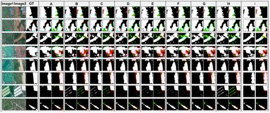
Figure 9.
Visualized performance comparison of different threshold partitioning schemes of the FDFR module on the CLCD dataset. (A–H denote different comparative settings, and I represents the proposed method).
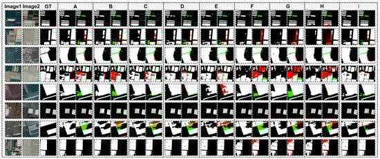
Figure 10.
Visualized performance comparison of different threshold partitioning schemes of the FDFR module on the Peixian dataset. (A–H denote different comparative settings, and I represents the proposed method).
First, an insufficient number of classes leads to inadequate discrimination of change intensity. As shown in Figure 9 and Figure 10 (A–C), in the 2-class schemes, the model can only divide change regions into “strong change” and “weak change” using a single threshold, failing to capture the distinctions among subtle, moderate, and significant changes. When a low threshold is used (e.g., scheme A), a large number of weak-change regions are included, resulting in improved Recall but a pronounced decrease in Precision, indicating that noise is mistakenly identified as true change. Conversely, when higher thresholds are adopted (schemes B and C), Precision improves, but subtle changes are missed, leading to a marked decline in Recall and consequently lower overall F1 and IoU scores. These observations indicate that 2-class partitioning is overly coarse and cannot balance the detection of changes with different intensities in complex scenarios.
Second, an excessive number of classes also introduces negative effects. As illustrated in Figure 9 and Figure 10 (F–H), the 5-class schemes provide more granular levels of change intensity; however, too many thresholds further subdivide weak-change regions, dispersing the model’s branch attention across multiple sub-intervals and leading to unstable representations. This issue is particularly evident in the CLCD dataset, which is characterized by complex textures and abundant noise, where the 5-class schemes yield the lowest Precision and IoU among all methods. Although slight improvements are observed on the relatively homogeneous Peixian dataset, the 5-class schemes still perform noticeably worse than the optimal configuration. This indicates that overly fine-grained change partitioning induces noise accumulation effects, thereby interfering with the model’s ability to focus on genuine changes.
In contrast, the 3-class scheme achieves a favorable balance between complexity and representational capacity. Nevertheless, the selection of threshold values remains critical. Among the three 3-class configurations, scheme D (0.1/0.5) sets an excessively high upper threshold, causing some significant changes to be misclassified as moderate changes, while scheme E (0.05/0.1) is overly biased toward weak changes, resulting in insufficient discrimination within change regions. Only the 0.1/0.3 configuration effectively covers both subtle and typical change intervals, thereby forming a more reasonable distribution of change intensity.
Specifically, the threshold of 0.1 effectively captures subtle variations induced by shadows and dark textures, which are ubiquitous in SAR imagery and contribute substantially to final recognition accuracy. Meanwhile, the threshold of 0.3 corresponds to a representative boundary in change intensity: regions below 0.3 are predominantly associated with noise disturbances or weak changes, whereas regions above 0.3 are more likely to represent genuine structural differences, such as water boundaries or pronounced land-cover changes. Because these two thresholds accurately partition change regions in both physical interpretation and statistical behavior, the 3-class scheme I achieves the optimal IoU, F1, and OA on both datasets.
4.3. Comparative Experiments
To comprehensively verify the effectiveness and superiority of the proposed FarmChanger (Farm.) model for cropland change detection, seven representative change detection networks were selected for comparison: ChangeFormer (ChangeF., 2022), TransUnetCD (Trans.CD., 2022), SNUNet (SNU., 2021), HANet (HA., 2022), CGNet (CG., 2021), HCGMNet (HCGM., 2023), and the latest state-of-the-art model HSANet (HSA., 2025). These models encompass mainstream design paradigms, including CNN-based architectures, Transformer-based architectures, CNN–Transformer hybrids, multi-scale fusion, attention mechanisms, and lightweight strategies, enabling a comprehensive validation of the proposed approach in terms of global modeling, boundary optimization, and multi-scale feature representation.
Table 5 presents the quantitative comparison of different models on the CLCD and Peixian datasets. Overall, the proposed model achieves the best performance on both datasets, particularly in terms of F1 and IoU scores, demonstrating its comprehensive advantages in multi-scale feature fusion, boundary optimization, and feature refinement.
Table 5.
Accuracy evaluation of comparison experiments (values in red bold indicate the best results within each dataset, while purple bold values denote the second-best results; “Effi.” represents Efficiency).
For the CLCD dataset, the F1 scores of the compared models range from 57.96% to 63.24%. As shown in the evaluation results, conventional CNN-based models (e.g., SNUNet, CGNet, HCGMNet) exhibit limited receptive fields and weak long-range dependency modeling, leading to frequent misclassification under large-scale farmland and complex background conditions. As illustrated in Figure 11, these models tend to produce evident false alarms and omissions in non-change regions. Transformer-based models such as ChangeFormer and TransUnetCD perform better in global feature modeling, achieving F1 scores of 61.88% and 59.10%, respectively. In contrast, the proposed FarmChanger achieves the highest F1 (63.24%), IoU (46.25%), and Kappa (60.29%) on the CLCD dataset, surpassing ChangeFormer by 1.36%, 1.44%, and 1.31%, respectively. The visual comparison in Figure 11 further confirms that FarmChanger effectively reduces omission and commission errors while preserving boundary completeness and clarity, achieving a superior balance between global dependency and local detail refinement.
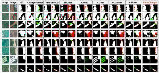
Figure 11.
Comparison of change detection results on the CLCD dataset (green areas indicate false detections, red areas indicate missed detections. The brown text indicates the proposed model in this work).
For the Peixian dataset, all models perform better than on CLCD due to its relatively uniform land-cover distribution and stable illumination conditions (Figure 12). Multi-scale and attention-based models (e.g., HANet, CGNet, HCGMNet, HSANet) show strong performance, with F1 scores exceeding 85%. Among them, HANet achieves an F1 of 87.06%, indicating that hierarchical attention mechanisms effectively handle farmland changes across scales. Nevertheless, FarmChanger further improves the results, achieving F1 = 88.87%, IoU = 79.97%, and Kappa = 87.21%, with both Precision and Recall exceeding 88%. As shown in Figure 12, FarmChanger exhibits superior stability in boundary integrity and semantic consistency, successfully balancing fine-grained detail extraction and overall structural coherence under complex surface conditions, outperforming existing state-of-the-art models in overall performance.
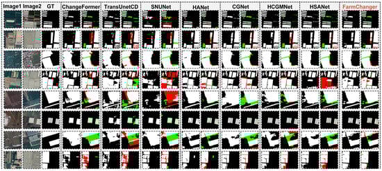
Figure 12.
Comparison of change detection results on the Peixian dataset (green areas indicate false detections, red areas indicate missed detections. The brown text indicates the proposed model in this work).
The confidence interval visualizations in Figure 13 and Figure 14 demonstrate the stability and reliability of FarmChanger’s performance across both the CLCD and Peixian datasets.
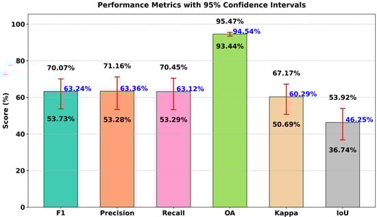
Figure 13.
Confidence intervals of FarmChanger on the CLCD dataset (numbers in black indicate the upper and lower bounds of the confidence intervals).
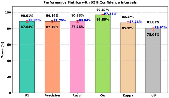
Figure 14.
Illustration of confidence intervals of FarmChanger on the Peixian dataset (numbers in black indicate the upper and lower bounds of the confidence intervals).
5. Conclusions
To address the challenges of multi-scale structure representation, pseudo-change interference, and boundary uncertainty in cultivated land change detection, this study proposes a lightweight diffusion-guided change detection network (FarmChanger). Through the collaborative integration of three core modules—MSAD, FDFR, and GSCA—the model achieves substantial improvements in multi-scale feature modeling, pseudo-change suppression, and fine-grained boundary reconstruction. Experimental results demonstrate that FarmChanger achieves superior and stable detection performance across datasets from different regions and with varying complexity, outperforming commonly used CNN- and Transformer-based models in key metrics such as F1 and IoU. However, although the model attains a good balance between accuracy and efficiency, minor misclassifications and omissions still occur under extreme illumination conditions and complex phenological variations. This indicates that current approaches relying on fixed attention structures and static scale modeling still exhibit certain limitations in complex remote sensing scenarios. In the future, the model’s generalization capability and practical applicability will be further enhanced by incorporating learnable attention scheduling mechanisms, adaptive scale-selection strategies, and the integration of multimodal and temporal information.
Author Contributions
Conceptualization, Y.C.; Methodology, Y.C.; Software, Y.C.; Validation, Y.C.; Formal analysis, Y.C.; Investigation, Y.C.; Resources, Y.C. and L.T.; Data curation, Y.C.; Writing—original draft, Y.C.; Writing—review & editing, S.Q., Y.Y., Z.L., W.Y., Y.Z. and L.T.; Visualization, Y.C.; Supervision, S.Q., Y.Y., Z.L., W.Y., Y.Z. and L.T.; Project administration, Y.C. and L.T.; Funding acquisition, Y.C. and L.T. All authors have read and agreed to the published version of the manuscript.
Funding
This research was funded by the Overseas Science and Education Cooperation Center under the project ‘Establishment of a Lunar Radiation Model’ (Project No. 178GJHZ2022056MI).
Data Availability Statement
The CropLand Change Detection (CLCD) Dataset is available from the GitHub repository at https://github.com/liumency/CropLand-CD (accessed on 6 August 2025). The Peixian Cultivated Land Change Detection Dataset (Peixian) can be obtained from https://github.com/niuzhan/Peixian-Cultivated-land-Change-detection-dataset (accessed on 16 August 2025).
Conflicts of Interest
The authors declare no conflict of interest.
References
- Zhu, Y.; Zhang, Y.; Ma, L.; Yu, L.; Wu, L. Simulating the dynamics of cultivated land use in the farming regions of China: A social-economic-ecological system perspective. J. Clean. Prod. 2024, 478, 143907. [Google Scholar] [CrossRef]
- Chen, J. Rapid urbanization in China: A real challenge to soil protection and food security. Catena 2007, 69, 1–15. [Google Scholar] [CrossRef]
- Zhao, Y.; Yuan, X.; Liu, Y. Understanding the transformation of rural areal system from changes in farmland landscape: A case study of Jiaocun township, Henan province. Habitat Int. 2025, 159, 103358. [Google Scholar] [CrossRef]
- Cheng, G.; Huang, Y.; Li, X.; Lyu, S.; Xu, Z.; Zhao, H.; Zhao, Q.; Xiang, S. Change detection methods for remote sensing in the last decade: A comprehensive review. Remote Sens. 2024, 16, 2355. [Google Scholar] [CrossRef]
- Yu, C.; Yang, H.; Ma, L.; Yang, J.; Jin, Y.; Zhang, W.; Wang, K.; Zhao, Q. Deep Learning-Based Change Detection in Remote Sensing: A Comprehensive Review. IEEE J. Sel. Top. Appl. Earth Obs. Remote Sens. 2025, 18, 24415–24437. [Google Scholar] [CrossRef]
- Jiang, H.; Peng, M.; Zhong, Y.; Xie, H.; Hao, Z.; Lin, J.; Ma, X.; Hu, X. A survey on deep learning-based change detection from high-resolution remote sensing images. Remote Sens. 2022, 14, 1552. [Google Scholar] [CrossRef]
- Tewkesbury, A.P.; Comber, A.J.; Tate, N.J.; Lamb, A.; Fisher, P.F. A critical synthesis of remotely sensed optical image change detection techniques. Remote Sens. Environ. 2015, 160, 1–14. [Google Scholar] [CrossRef]
- Omia, E.; Bae, H.; Park, E.; Kim, M.S.; Baek, I.; Kabenge, I.; Cho, B.-K. Remote sensing in field crop monitoring: A comprehensive review of sensor systems, data analyses and recent advances. Remote Sens. 2023, 15, 354. [Google Scholar] [CrossRef]
- Wan, L.; Xiang, Y.; You, H. A post-classification comparison method for SAR and optical images change detection. IEEE Geosci. Remote Sens. Lett. 2019, 16, 1026–1030. [Google Scholar] [CrossRef]
- Liu, H.; Zhou, Q. Accuracy analysis of remote sensing change detection by rule-based rationality evaluation with post-classification comparison. Int. J. Remote Sens. 2004, 25, 1037–1050. [Google Scholar] [CrossRef]
- Zhu, Q.; Guo, X.; Li, Z.; Li, D. A review of multi-class change detection for satellite remote sensing imagery. Geo-Spat. Inf. Sci. 2024, 27, 1–15. [Google Scholar] [CrossRef]
- Zhou, Z.; Hu, K.; Fang, Y.; Rui, X. SChanger: Change Detection from a Semantic Change and Spatial Consistency Perspective. IEEE J. Sel. Top. Appl. Earth Obs. Remote Sens. 2025, 18, 10186. [Google Scholar] [CrossRef]
- Han, C.; Wu, C.; Guo, H.; Hu, M.; Li, J.; Chen, H. Change guiding network: Incorporating change prior to guide change detection in remote sensing imagery. IEEE J. Sel. Top. Appl. Earth Obs. Remote Sens. 2023, 16, 8395–8407. [Google Scholar] [CrossRef]
- Long, J.; Shelhamer, E.; Darrell, T. Fully convolutional networks for semantic segmentation. In Proceedings of the IEEE Conference on Computer Vision and Pattern Recognition, San Francisco, CA, USA, 18–20 June 1996; pp. 3431–3440. [Google Scholar]
- Ronneberger, O.; Fischer, P.; Brox, T. U-net: Convolutional Networks for Biomedical Image Segmentation; Springer: Cham, Switzerland, 2015; pp. 234–241. [Google Scholar]
- Zhang, C.; Wei, S.; Ji, S.; Lu, M. Detecting large-scale urban land cover changes from very high resolution remote sensing images using CNN-based classification. ISPRS Int. J. Geo-Inf. 2019, 8, 189. [Google Scholar] [CrossRef]
- Micallef, N.; Seychell, D.; Bajada, C.J. Exploring the u-net++ model for automatic brain tumor segmentation. IEEE Access 2021, 9, 125523–125539. [Google Scholar] [CrossRef]
- Peng, D.; Zhang, Y.; Guan, H. End-to-end change detection for high resolution satellite images using improved UNet++. Remote Sens. 2019, 11, 1382. [Google Scholar] [CrossRef]
- Saidi, S.; Idbraim, S.; Karmoude, Y.; Masse, A.; Arbelo, M. Deep-learning for change detection using multi-modal fusion of remote sensing images: A review. Remote Sens. 2024, 16, 3852. [Google Scholar] [CrossRef]
- Touati, R.; Mignotte, M.; Dahmane, M. Partly uncoupled siamese model for change detection from heterogeneous remote sensing imagery. J. Remote Sens. GIS 2020, 9, 1–8. [Google Scholar]
- Xu, Q.; Chen, K.; Sun, X.; Zhang, Y.; Li, H.; Xu, G. Pseudo-Siamese capsule network for aerial remote sensing images change detection. IEEE Geosci. Remote Sens. Lett. 2020, 19, 1–5. [Google Scholar] [CrossRef]
- Farhadi, N.; Kiani, A.; Ebadi, H. OctaveNet: An efficient multi-scale pseudo-siamese network for change detection in remote sensing images. Multimed. Tools Appl. 2024, 83, 83941–83961. [Google Scholar] [CrossRef]
- Yang, K.; Xia, G.-S.; Liu, Z.; Du, B.; Yang, W.; Pelillo, M.; Zhang, L. Asymmetric siamese networks for semantic change detection in aerial images. IEEE Trans. Geosci. Remote Sens. 2021, 60, 1–18. [Google Scholar] [CrossRef]
- Jiang, H.; Hu, X.; Li, K.; Zhang, J.; Gong, J.; Zhang, M. PGA-SiamNet: Pyramid feature-based attention-guided Siamese network for remote sensing orthoimagery building change detection. Remote Sens. 2020, 12, 484. [Google Scholar] [CrossRef]
- Wang, M.; Tan, K.; Jia, X.; Wang, X.; Chen, Y. A deep siamese network with hybrid convolutional feature extraction module for change detection based on multi-sensor remote sensing images. Remote Sens. 2020, 12, 205. [Google Scholar] [CrossRef]
- Yan, W.; Cao, L.; Yan, P.; Zhu, C.; Wang, M. Remote sensing image change detection based on swin transformer and cross-attention mechanism. Earth Sci. Inform. 2025, 18, 106. [Google Scholar] [CrossRef]
- Yan, T.; Wan, Z.; Zhang, P. Fully Transformer Network for Change Detection of Remote Sensing Images; Springer: Cham, Switzerland, 2022; pp. 1691–1708. [Google Scholar]
- Liu, M.; Chai, Z.; Deng, H.; Liu, R. A CNN-transformer network with multiscale context aggregation for fine-grained cropland change detection. IEEE J. Sel. Top. Appl. Earth Obs. Remote Sens. 2022, 15, 4297–4306. [Google Scholar] [CrossRef]
- Chen, Y.; Liu, P.; Zhao, J.; Huang, K.; Yan, Q. Shallow-guided transformer for semantic segmentation of hyperspectral remote sensing imagery. Remote Sens. 2023, 15, 3366. [Google Scholar] [CrossRef]
- Li, G.; Huang, Q.; Wang, W.; Liu, L. Selective and multi-scale fusion mamba for medical image segmentation. Expert Syst. Appl. 2025, 261, 125518. [Google Scholar] [CrossRef]
- Cai, S.; Jiang, Y.; Xiao, Y.; Zeng, J.; Zhou, G. TransUMobileNet: Integrating multi-channel attention fusion with hybrid CNN-Transformer architecture for medical image segmentation. Biomed. Signal Process. Control 2025, 107, 107850. [Google Scholar] [CrossRef]
- Xie, Y.; Rui, X.; Zou, Y.; Tang, H.; Ouyang, N.; Ren, Y. STDPNet: Supervised transformer-driven network for high-precision oil spill segmentation in SAR imagery. Int. J. Appl. Earth Obs. Geoinf. 2025, 143, 104812. [Google Scholar] [CrossRef]
- Chen, Y.; Xie, Y.; Yao, W.; Zhang, Y.; Wang, X.; Yang, Y.; Tang, L. U-mga: A multi-module unet optimized with multi-scale global attention mechanisms for fine-grained segmentation of cultivated areas. Remote Sens. 2025, 17, 760. [Google Scholar] [CrossRef]
- Xie, Y.; Zhang, H.; Rui, X.; Tang, H.; Ouyang, N.; Zou, Y. MSAttU-Net: A water body extraction network for Nanjing that overcomes interference in shaded areas. IEEE Geosci. Remote Sens. Lett. 2025, 22, 1–5. [Google Scholar] [CrossRef]
- Han, C.; Wu, C.; Du, B. HCGMNet: A hierarchical change guiding map network for change detection. In Proceedings of the IGARSS 2023 IEEE International Geoscience and Remote Sensing Symposium, Pasadena, CA, USA, 16–21 July 2023; pp. 5511–5514. [Google Scholar]
- Thonfeld, F. The Impact of Sensor Characteristics and Data Availability on Remote Sensing Based Change Detection. Ph.D. Thesis, Rheinische Friedrich-Wilhelms-Universität Bonn, Bonn, Germany, 2014. [Google Scholar]
- Shafique, A.; Cao, G.; Khan, Z.; Asad, M.; Aslam, M. Deep learning-based change detection in remote sensing images: A review. Remote Sens. 2022, 14, 871. [Google Scholar] [CrossRef]
- Huang, Y.; Li, X.; Du, Z.; Shen, H. Spatiotemporal enhancement and interlevel fusion network for remote sensing images change detection. IEEE Trans. Geosci. Remote Sens. 2024, 62, 1–14. [Google Scholar] [CrossRef]
- Guo, Z.; Chen, H.; He, F. MSFNet: Multi-scale Spatial-frequency Feature Fusion Network for Remote Sensing Change Detection. IEEE J. Sel. Top. Appl. Earth Obs. Remote Sens. 2024, 18, 1912–1925. [Google Scholar] [CrossRef]
- Cao, H.; Tan, C.; Gao, Z.; Xu, Y.; Chen, G.; Heng, P.-A.; Li, S.Z. A survey on generative diffusion models. IEEE Trans. Knowl. Data Eng. 2024, 36, 2814–2830. [Google Scholar] [CrossRef]
- Wu, J.; Fu, R.; Fang, H.; Zhang, Y.; Yang, Y.; Xiong, H.; Liu, H.; Xu, Y. Medsegdiff: Medical image segmentation with diffusion probabilistic model. Proc. Mach. Learn. Res. 2022, 227, 1623–1639. [Google Scholar]
- Wu, J.; Ji, W.; Fu, H.; Xu, M.; Jin, Y.; Xu, Y. Medsegdiff-v2: Diffusion-based medical image segmentation with transformer. In Proceedings of the AAAI Conference on Artificial Intelligence, Washington, DC, USA, 25 February–4 March 2025; pp. 6030–6038. [Google Scholar]
- Xing, Z.; Wan, L.; Fu, H.; Yang, G.; Yang, Y.; Yu, L.; Lei, B.; Zhu, L. Diff-UNet: A diffusion embedded network for robust 3D medical image segmentation. Med. Image Anal. 2025, 105, 103654. [Google Scholar] [CrossRef]
- Amit, T.; Shaharbany, T.; Nachmani, E.; Wolf, L. Segdiff: Image segmentation with diffusion probabilistic models. arXiv 2021, arXiv:2112.00390. [Google Scholar]
- Baranchuk, D.; Rubachev, I.; Voynov, A.; Khrulkov, V.; Babenko, A. Label-efficient semantic segmentation with diffusion models. arXiv 2021, arXiv:2112.03126. [Google Scholar]
- Miao, L.; Li, X.; Zhou, X.; Yao, L.; Deng, Y.; Hang, T.; Zhou, Y.; Yang, H. SNUNet3+: A full-scale connected Siamese network and a dataset for cultivated land change detection in high-resolution remote-sensing images. IEEE Trans. Geosci. Remote Sens. 2023, 62, 1–18. [Google Scholar] [CrossRef]
- Wen, Y.; Zhang, Z.; Cao, Q.; Niu, G. Transc-gd-cd: Transformer-based conditional generative diffusion change detection model. IEEE J. Sel. Top. Appl. Earth Obs. Remote Sens. 2024, 17, 7144–7158. [Google Scholar] [CrossRef]
- Bandara, W.G.C.; Nair, N.G.; Patel, V.M. DDPM-CD: Denoising diffusion probabilistic models as feature extractors for remote sensing change detection. In Proceedings of the 2025 IEEE/CVF Winter Conference on Applications of Computer Vision (WACV), Tucson, AZ, USA, 26 February–6 March 2025; pp. 5250–5262. [Google Scholar]
- Wang, W.; Su, Q.; Wang, X. DDECNet: Dual-Branch Difference Enhanced Network with Novel Efficient Cross-Attention for Remote Sensing Change Detection; Springer: Singapore, 2025; pp. 125–136. [Google Scholar]
- Li, F.; Zhang, C.; Zhang, X.; Li, Y. MF-DCMANet: A multi-feature dual-stage cross manifold attention network for PolSAR target recognition. Remote Sens. 2023, 15, 2292. [Google Scholar] [CrossRef]


Disclaimer/Publisher’s Note: The statements, opinions and data contained in all publications are solely those of the individual author(s) and contributor(s) and not of MDPI and/or the editor(s). MDPI and/or the editor(s) disclaim responsibility for any injury to people or property resulting from any ideas, methods, instructions or products referred to in the content. |
© 2025 by the authors. Licensee MDPI, Basel, Switzerland. This article is an open access article distributed under the terms and conditions of the Creative Commons Attribution (CC BY) license.