Model–Data Dual-Driven Method for Mode-Switching Radar Target Detection

Highlights

What are the main findings?

• An innovative model-data dual-driven framework is proposed, effectively addressing the degradation of radar detection performance caused by mode-switching in highly maneuvering targets.
• An interpretable hierarchical residual network is designed, which accurately infers the target’s initial and switch points, while its decision-making rationale is revealed through visualization techniques.

What are the implications of the main findings?

• This study provides a new method with superior performance and higher efficiency for radar detection of complex maneuvering targets, which can be directly applied to the precise tracking and identification of high-speed targets such as fighter aircraft and missiles.
• The proposed dual-driven framework and interpretable network design offer a general methodological reference for handling other signal processing problems involving uncertain mode-switching.

Abstract

Maneuvering targets exhibit range migration (RM) and Doppler-frequency migration (DFM) during the coherent integration period. Most existing coherent integration methods model maneuvering target motion with a single motion mode. However, highly maneuvering targets often undergo mode-switching, which degrades the detection performance of conventional algorithms. To address this problem, this paper proposes a model–data dual-driven method for mode-switching radar targets. From the model-driven perspective, the range evolution over time is derived in the Cartesian coordinate system for transitions among constant-velocity (CV), constant-acceleration (CA), and constant-turn (CT) motions, thereby constructing multiple possible mode-switching scenarios. Subsequently, from the data-driven perspective, a hierarchical residual network and keypoint loss functions are designed to learn and capture the uncertainty associated with mode-switching, thereby accurately inferring the initial and switching points of the target. Furthermore, to enhance the interpretability of the network, probability heatmap visualization is employed to intuitively reveal the internal mechanisms of the network. Finally, by partitioning the Coherent Processing Interval (CPI) based on network-detected keypoints, the proposed method performs efficient piecewise coherent integration for different motion models by integrating along the slow-time echo-envelope migration path. Simulation results demonstrate that the proposed method not only effectively eliminates both RM and DFM but also achieves strong detection performance and favorable computational efficiency.

1. Introduction

Radar, as the core equipment of modern sensing systems, plays an indispensable role in various domains, including military defense, civil aviation, maritime surveillance, and meteorological observation. With its all-weather and all-time operating capability, radar enables high-precision detection and continuous tracking of airborne and maritime targets, thereby serving as a critical technological support for national security and societal needs. In the aerospace domain, high-speed maneuvering targets in near-space environments impose more stringent requirements and challenges on radar detection performance. Such targets are characterized by high maneuverability and low observability, rendering conventional radar architectures and signal processing methods ineffective for reliable detection. Consequently, breaking through the limitations of existing signal processing theories, exploring new radar processing mechanisms, and enhancing radar capability against high-speed maneuvering targets have become pressing scientific issues that must be addressed. For radar systems, waveforms with a large time–bandwidth product are typically employed to enhance range resolution and detection accuracy. However, due to the motion characteristics of high-speed maneuvering targets, which may migrate across multiple range and Doppler cells within the coherent processing interval (CPI), the performance of conventional detection algorithms can degrade significantly [1,2,3,4]. Consequently, achieving effective coherent integration in the signal domain has become a critical and challenging problem.

From the perspective of signal processing, pulse integration methods can be categorized into noncoherent integration and coherent integration depending on whether phase information is used. Coherent integration utilizes both amplitude and phase, whereas noncoherent integration relies only on amplitude. Noncoherent integration approaches include the maximum likelihood method, the Hough transform [5,6,7], and dynamic programming. Compared with coherent integration, noncoherent integration is easier to implement in engineering practice but yields lower energy-accumulation efficiency and smaller signal-to-noise ratio (SNR) gains. The mechanism of coherent integration is to compensate for inter-pulse phase fluctuations so that the signals add in phase, thereby achieving efficient energy accumulation. Nevertheless, current coherent integration methods face two issues. First, with the emergence of highly maneuvering targets and the improvement of radar range resolution, the envelope of the target echo crosses range bins over the integration time, i.e., range migration [8], which appears as energy dispersion in the range–pulse domain. Second, target acceleration or higher-order maneuvers induce highly nonlinear phase variations in the echoes, causing energy to disperse across multiple Doppler bins during the integration time, i.e., Doppler migration [9]. Unfortunately, the traditional moving target detection (MTD) algorithm is no longer adequate to handle these situations. To address these problems, many researchers and research teams have proposed a series of solutions. Perry et al. [10,11] introduced the Keystone transform (KT), which corrects RM by performing range–frequency scaling. This approach is applicable to multi-target and low-SNR scenarios and can effectively eliminate RM caused by target radial velocity. However, it fails to correct the range curvature induced by target radial acceleration [12]. Envelope-correlation methods [13], such as the cross-correlation method, minimum-entropy method, and spectral-peak tracking method, are also commonly used for coherent integration. Nevertheless, these methods perform poorly under low-SNR conditions, as weak correlation between adjacent echoes prevents accurate envelope alignment. Other classical multi-pulse integration methods, such as the sequential cross transform [14,15] and the scaled inverse Fourier transform [16,17], reduce computational cost at the expense of detection performance. The Radon–Fourier transform (RFT) [8] performs a joint search over the parameter space to handle both RM and DFM, but it is applicable only when the radial range varies linearly. To overcome this limitation, the generalized Radon–Fourier transform (GRFT) [18] was proposed, extending its applicability to more complex target motions. However, the associated parameter-space search is computationally intensive, limiting its engineering practicality. The short-time generalized Radon–Fourier transform (STGRFT) [19] further improves detection performance for maneuvering targets, but the additional filtering substantially increases computational complexity. Traditional coherent integration methods can be viewed as model-driven approaches that struggle to balance computational cost and detection performance and thus hamper further development. Moreover, most existing methods rely on a single motion model assumption and fail to account for mode-switching, thereby limiting detection capabilities in complex maneuvering scenarios.

The rapid advancement of deep learning and computing power has markedly accelerated progress in computer vision and natural language processing. Deep convolutional neural networks (CNNs) have achieved notable breakthroughs in optical-image target detection. Since 2010, applications of deep learning to radar datasets have received increasing attention. Early research focused primarily on classification and recognition of synthetic aperture radar (SAR) imagery and subsequently expanded to radar target detection and tracking. Compared with traditional methods that require handcrafted feature extraction, deep learning-based detectors provide superior automatic feature extraction and representation capabilities. Wang et al. [20] proposed a semi-supervised detection framework that improves the generalization of target detectors. Su et al. [21] introduced a method based on a spatiotemporal attention graph convolutional network operating on radar echoes. In this framework, multi-frame radar echoes are converted into graph signals to enable target detection in cluttered backgrounds, thereby enhancing detection performance. Yan et al. [22] combined a deep neural network with conventional coherent integration methods for maneuvering target detection, achieving improvements in both detection accuracy and the precision of parameter estimation. Jiang et al. [23] developed a fast parameter estimation approach using a residual network, attaining better detection performance with reduced computational complexity. Wang et al. [24] employed a fully convolutional network (FCN) to perform target trajectory detection and accumulated target energy along the detected trajectory, achieving a favorable balance between detection performance and computational complexity. Our research group has also contributed to improving target trajectory detection accuracy and network interpretability [25], further enhancing overall detection performance. In summary, the aforementioned deep learning-based radar target detection approaches can be regarded as data-driven methods with limited model-driven components. However, existing coherent integration methods face three key issues. First, most of these methods assume that the target follows a single motion mode within the observation period, i.e., only one kinematic state exists. Second, they typically employ polynomial signal models without accounting for the intrinsic characteristics of target motion. For instance, when the target performs constant-turn or circular maneuvers, conventional polynomial modeling fails to accurately describe such motion patterns, leading to model mismatch and detection performance degradation. Third, current studies still lack a unified framework that combines the advantages of both data-driven and model-driven paradigms, particularly for modeling targets with complex maneuvering behaviors involving mode-switching. Such hybrid approaches have been widely recognized and actively explored in other target detection domains [26,27,28,29].

Motivated by the aforementioned analysis, this paper proposes a model–data dual-driven method for mode-switching radar target detection. The model-driven component establishes precise kinematic representations of various motion modes and their spatial transitions, thereby enhancing detection robustness against maneuvering targets. Conversely, the data-driven component leverages a deep network trained on diverse motion trajectories, utilizing specialized loss functions to capture both the regularity and stochasticity of target motion. Fundamentally, detection performance hinges on the quality of feature representation. To this end, a multi-scale feature extraction network is developed to learn a nonlinear mapping from noisy radar echoes to target trajectories. This facilitates the accurate estimation of initial states and mode-switching instants, which are subsequently used to partition the coherent integration interval. Following this, parametric phase compensation and an energy-maximization criterion are applied to achieve effective coherent integration. Furthermore, to enhance interpretability, probability heatmap visualizations are employed to elucidate the network’s internal decision-making mechanisms. The main contributions of this article are summarized as follows:

(1) Construction of a comprehensive kinematic trajectory dataset for mode-switching targets. As described in [30,31,32], the CV model, the CT model, and their combinations can characterize target maneuverability. Building on this, we extend the dataset to include a richer set of motion models—namely CV, CT, CA, and their combinations—for mode-switching scenarios. This design captures a broad spectrum of real-world kinematics, thereby enhancing the generalization capability and detection performance of the proposed method.

(2) Development of a multi-scale feature extraction network. We develop a network architecture based on multi-scale feature extraction: shallow features are extracted using large convolutional kernels of different sizes, while deep features are extracted via multiple residual submodules. During the training process, classification and localization losses are jointly optimized for the initial points and mode-switching (switch) points of the target trajectories. This enables the network to learn robust feature representations, significantly improving the estimation accuracy of these keypoints.

(3) Enhanced interpretability via network output visualization. In the range-pulse spectrum, the keypoints identified by the network are highlighted with high posterior probabilities, yielding clear spectral-peak indications. This visualization not only facilitates the verification of initial and switching instants but also localizes candidate intervals for coherent integration, providing explicit guidance for subsequent parametric phase compensation.

(4) Efficient piecewise coherent integration strategy. Utilizing the keypoints estimated by the network, the CPI is adaptively partitioned into sub-intervals corresponding to distinct motion modes. Coherent integration is then achieved by performing phase compensation for the remaining motion parameters followed by an energy-maximization criterion. Consequently, the detrimental effects of both RM and DFM are effectively mitigated.

The remainder of this paper is organized as follows. Section 2 presents the signal model. Section 3 details the proposed method. Section 4 provides the simulation results and discussion. Section 5 concludes the paper.

2. Methodology

In a fully coherent pulse radar system, the linear frequency modulated (LFM) signal is commonly employed as the baseband waveform for target detection. Suppose that M pulses are transmitted during the detection period. the signal model of the m-th pulse can be expressed as follows:

$$S_t\left(\widehat{t},t_m\right)=rect\left({\displaystyle \frac{\widehat{t}}{T_p}}\right)\exp \left(j\pi \mu {\widehat{t}}^2\right)\exp \left[j2\pi f_c\left(\widehat{t}+t_m\right)\right]$$

(1)

where $rect\left(x\right)=\left\{\begin{array}{cc}1& \left|x\right|\le 0.5\\ 0& \left|x\right|>0.5\end{array}\right.$ denotes the rectangle window function. $j=\sqrt{-1}$ is the imaginary unit. The fast time and the slow time are denoted as $\widehat{t}$ and $t_m$, respectively. $t_m=m\times T_r(m=0,1,\dots ,M-1)$, where $T_r$ denotes the pulse repetition time. The coherent integration time is $T_{\mathrm{CPI}}=M\times T_r$. The frequency modulation rate is $\mu$, which can be expressed as $\mu =B/T_p$. $T_p$ and B denote the pulse duration and bandwidth, respectively. The carrier frequency is $f_c$.

During the observation period, let the instantaneous radial distance between the radar and the maneuvering target be denoted by $r\left(t_m\right)$. Then, the received baseband echo can be written as:

$$S_{\mathrm{r}}\left(\widehat{t},t_m\right)=A_{\mathrm{r}}rect\left({\displaystyle \frac{\widehat{t}-\raisebox{1ex}{$2r\left(t_m\right)$}\!\left/ \!\raisebox{-1ex}{$c$}\right.}{T_p}}\right)\exp \left[j\pi \mu {\left(\widehat{t}-{\displaystyle \frac{2r\left(t_m\right)}{c}}\right)}^2\right]\exp \left(-j4\pi {\displaystyle \frac{r\left(t_m\right)}{\lambda }}\right)$$

(2)

where $A_{\mathrm{r}}$ stands for the amplitude of echo. $\lambda$ denotes the wavelength. c is the light speed.

After pulse compression (PC), the range-compressed signal can be expressed as:

$$S_{\mathrm{cs}}(\widehat{t},t_m)=A_{\mathrm{cs}}\mathrm{sinc}\left[B\left(\widehat{t}-{\displaystyle \frac{2r\left(t_m\right)}{c}}\right)\right.\exp \left(-j{\displaystyle \frac{4\pi r\left(t_m\right)}{\lambda }}\right)$$

(3)

where $A_{\mathrm{cs}}$ indicates the amplitude of compressed signal.

3. Proposed Method

3.1. Target Trajectory Dataset Generation

Assume that the initial Cartesian position is ($p_{x,0}^{\mathrm{CV}},p_{y,0}^{\mathrm{CV}}$), and the velocity of target is ($v_x^{\mathrm{CV}},v_y^{\mathrm{CV}}$). Therefore, the instantaneous position of a CV target in the x and y directions are:

$$\begin{array}{cc}\hfill & p_x^{\mathrm{CV}}\left(t_m\right)=p_{x,0}^{\mathrm{CV}}+v_x^{\mathrm{CV}}{t}_m\hfill \\ \hfill & p_y^{\mathrm{CV}}\left(t_m\right)=p_{y,0}^{\mathrm{CV}}+v_y^{\mathrm{CV}}{t}_m.\hfill \end{array}$$

(4)

Then, according to $r_{\mathrm{CV}}\left(t_m\right)=\sqrt{{\left(p_x^{\mathrm{CV}}\left(t_m\right)\right)}^2+{\left(p_y^{\mathrm{CV}}\left(t_m\right)\right)}^2}$, the target instantaneous range $r_{\mathrm{CV}}\left(t_m\right)$ within the observation period can be expressed as:

$$\begin{array}{c}\hfill r_{\mathrm{CV}}\left(t_m\right)=\sqrt{r_{\mathrm{CV},0}^2+2r_{\mathrm{CV},0}{\dot{r}}_{\mathrm{CV},0}{t}_m+v_{\mathrm{CV},0}^2{t}_m^2}\end{array}$$

(5)

where $r_{\mathrm{CV},0}=\sqrt{{p_{x,0}^{\mathrm{CV}}}^2+{p_{y,0}^{\mathrm{CV}}}^2}$ denotes the initial range, ${\dot{r}}_{\mathrm{CV},0}=\left(p_{x,0}^{\mathrm{CV}}{v}_x^{\mathrm{CV}}+p_{y,0}^{\mathrm{CV}}{v}_y^{\mathrm{CV}}\right)/r_{\mathrm{CV},0}$ denotes the target’s radial velocity (relative to the radar) at the initial time, $v_{\mathrm{CV}}=\sqrt{{v_x^{\mathrm{CV}}}^2+{v_y^{\mathrm{CV}}}^2}$ denotes the absolute value of the target’s velocity.

Similarly, assume that the initial Cartesian position is $(p_{x,0}^{\mathrm{CT}},p_{y,0}^{\mathrm{CT}})$, the velocity of target is $(v_x^{\mathrm{CT}},v_y^{\mathrm{CT}})$, and the turn rate is ${\omega }_{\mathrm{CT},0}$. Therefore, the instantaneous position of a CT target in the x and y directions are:

$$\begin{array}{cc}\hfill & p_x^{\mathrm{CT}}\left(t_m\right)=p_{x,0}^{\mathrm{CT}}+{\displaystyle \frac{\sin {\omega }_{\mathrm{CT},0}{t}_m}{{\omega }_{\mathrm{CT},0}}}{v}_x^{\mathrm{CT}}-{\displaystyle \frac{1-\cos {\omega }_{\mathrm{CT},0}{t}_m}{{\omega }_{\mathrm{CT},0}}}{v}_y^{\mathrm{CT}}\hfill \\ \hfill & p_y^{\mathrm{CT}}\left(t_m\right)=p_{y,0}^{\mathrm{CT}}+{\displaystyle \frac{1-\cos {\omega }_{\mathrm{CT},0}{t}_m}{{\omega }_{\mathrm{CT},0}}}{v}_x^{\mathrm{CT}}+{\displaystyle \frac{\sin {\omega }_{\mathrm{CT},0}{t}_m}{{\omega }_{\mathrm{CT},0}}}{v}_y^{\mathrm{CT}}.\hfill \end{array}$$

(6)

Then, according to $r_{\mathrm{CT}}\left(t_m\right)=\sqrt{{\left(p_x^{\mathrm{CT}}\left(t_m\right)\right)}^2+{\left(p_y^{\mathrm{CT}}\left(t_m\right)\right)}^2}$, the target instantaneous range $r_{\mathrm{CT}}\left(t_m\right)$ within the observation period can be expressed as:

$$\begin{array}{c}\hfill r_{\mathrm{CT}}\left(t_m\right)=\sqrt{r_{\mathrm{CT},0}^2+{\displaystyle \frac{2\sin {\omega }_{\mathrm{CT},0}{t}_m}{{\omega }_{\mathrm{CT},0}}}{r}_{\mathrm{CT},0}{\dot{r}}_{\mathrm{CT},0}+{\displaystyle \frac{2\left(1-\cos {\omega }_{\mathrm{CT},0}{t}_m\right)}{{\omega }_{\mathrm{CT},0}^2}}{\sigma }_{\mathrm{CT},0}}\end{array}$$

(7)

where $r_{\mathrm{CT},0}=\sqrt{{\left(p_{x,0}^{\mathrm{CT}}\right)}^2+{\left(p_{y,0}^{\mathrm{CT}}\right)}^2}$ denotes the initial range. ${\dot{r}}_{\mathrm{CT},0}=\raisebox{1ex}{$\left(p_{x,0}^{\mathrm{CT}}{v}_x^{\mathrm{CT}}+p_{y,0}^{\mathrm{CT}}{v}_y^{\mathrm{CT}}\right)$}\!\left/ \!\raisebox{-1ex}{$r_{\mathrm{CT},0}$}\right.$ denotes the target’s radial velocity. ${\sigma }_{\mathrm{CT},0}={\left(v_x^{\mathrm{CT}}\right)}^2+{\left(v_y^{\mathrm{CT}}\right)}^2+{\omega }_{\mathrm{CT},0}\left(p_{y,0}^{\mathrm{CT}}{v}_x^{\mathrm{CT}}-p_{x,0}^{\mathrm{CT}}{v}_y^{\mathrm{CT}}\right)$ is introduced via a variable substitution. Since it is of the same order as the squared velocity, it is referred to as the pseudo velocity.

Likewise, assume that the initial Cartesian position is $(p_{x,0}^{\mathrm{CA}},p_{y,0}^{\mathrm{CA}})$; the velocity of the target is $(v_x^{\mathrm{CA}},v_y^{\mathrm{CA}})$, and the acceleration of the target is $(a_x^{\mathrm{CA}},a_y^{\mathrm{CA}})$. Therefore, the instantaneous position of a CA target in the x and y directions are:

$$\begin{array}{cc}\hfill & p_x^{\mathrm{CA}}\left(t_m\right)=p_{x,0}^{\mathrm{CA}}+v_x^{\mathrm{CA}}{t}_m+{\displaystyle \frac{1}{2}}{a}_x^{\mathrm{CA}}{t}_m^2\hfill \\ \hfill & p_y^{\mathrm{CA}}\left(t_m\right)=p_{y,0}^{\mathrm{CA}}+v_y^{\mathrm{CA}}{t}_m+{\displaystyle \frac{1}{2}}{a}_y^{\mathrm{CA}}{t}_m^2.\hfill \end{array}$$

(8)

Then, according to $r_{\mathrm{CA}}\left(t_m\right)=\sqrt{{\left(p_x^{\mathrm{CA}}\left(t_m\right)\right)}^2+{\left(p_y^{\mathrm{CA}}\left(t_m\right)\right)}^2}$, the target instantaneous range $r_{\mathrm{CA}}\left(t_m\right)$ within the observation period can be expressed as:

$$r_{\mathrm{CA}}\left(t_m\right)=\sqrt{\begin{array}{c}{r}_{\mathrm{CA},0}^2+2r_{\mathrm{CA},0}{v}_{\mathrm{CA}}\cos {\theta }_{\dot{r}v,0}{t}_m+\left(v_{\mathrm{CA},0}^2+r_{\mathrm{CA},0}{a}_{\mathrm{CA},0}\cos {\theta }_{va,0}\cos {\theta }_{\dot{r}v,0}\right)t_m^2\hfill \\ +v_{\mathrm{CA},0}{a}_{\mathrm{CA},0}\cos {\theta }_{va,0}{t}_m^3+0.25a_{\mathrm{CA},0}^2{t}_m^4.\hfill \end{array}}$$

(9)

where $r_{\mathrm{CA},0}=\sqrt{{\left(p_{x,0}^{\mathrm{CA}}\right)}^2+{\left(p_{y,0}^{\mathrm{CA}}\right)}^2}$ denotes the initial range. The angle between the target’s velocity and acceleration is defined as ${\theta }_{va}$ in the Cartesian coordinate system, then when the target executes CA motion, the velocity and acceleration vectors satisfy the collinearity condition, i.e., ${\theta }_{va,0}=0$ or $\pi$. Meanwhile, the angle between the target’s velocity and radial velocity is denoted as ${\theta }_{\dot{r}v,0}=[0,\pi ]$. $v_{\mathrm{CA},0}=\sqrt{{\left(v_x^{\mathrm{CA}}\right)}^2+{\left(v_y^{\mathrm{CA}}\right)}^2}$ denotes the absolute value of the target’s velocity, and the relationship between the target’s radial velocity and velocity can be expressed as ${\dot{r}}_{\mathrm{CA},0}=v_{\mathrm{CA},0}\cos {\theta }_{\dot{r}v,0}$. $a_{\mathrm{CA},0}=\sqrt{{\left(a_x^{\mathrm{CA}}\right)}^2+{\left(a_y^{\mathrm{CA}}\right)}^2}$ denotes the absolute value of the target’s acceleration.

By forming diverse combinations of the three basic motion types, we comprehensively cover potential mode-switching behaviors observed in practice.

Table 1. Mode-switching behaviors observed in practice.

Case	Mode-Switching	Case	Mode-Switching
Case 1	CVCA	Case 4	CACT
Case 2	CACV	Case 5	CVCT
Case 3	CTCA	Case 6	CTCV

shows the details. It is worth noting that Case 5 and Case 6 have been discussed in previous work [32]. Therefore, the following analysis focuses on Cases 1–4. Take Case 1 as an example; Case 1 indicates that the target first executes a segment of CV motion followed by a segment of CA motion, with the mode-switching occurring at an arbitrary pulse.

Case 1: the target first executes a segment of CV motion followed by a segment of CA motion, with the mode-switching occurring at $t_{\gamma }$, which can be expressed as follows:

$$\begin{array}{c}\hfill r_{\mathrm{CVCA}}\left(t_m\right)=\left\{\begin{array}{cccc}& \sqrt{r_{\mathrm{CV},0}^2+2r_{\mathrm{CV},0}{\dot{r}}_{\mathrm{CV},0}{t}_m+v_{\mathrm{CV},0}^2{t}_m^2},& & 0\le t_m\le t_{\gamma }\\ & \sqrt{\begin{array}{c}{r}_{\mathrm{CA},t_{\gamma }}^2+2r_{\mathrm{CA},t_{\gamma }}{v}_{\mathrm{CA},t_{\gamma }}\cos {\theta }_{\dot{r}v,t_{\gamma }}{t}_m\hfill \\ +\left(v_{\mathrm{CA},t_{\gamma }}^2+a_{\mathrm{CA},t_{\gamma }}{r}_{\mathrm{CA},t_{\gamma }}\cos {\theta }_{va,t_{\gamma }}\cos {\theta }_{\dot{r}v,t_{\gamma }}\right)t_m^2\hfill \\ +\cos {\theta }_{va,t_{\gamma }}{v}_{\mathrm{CA},t_{\gamma }}{a}_{\mathrm{CA},t_{\gamma }}{t}_m^3+0.25a_{\mathrm{CA},t_{\gamma }}^2{t}_m^4\hfill \end{array}},& & t_{\gamma }<t_m\le t_{M-1}.\end{array}\right.\end{array}$$

(10)

Case 2: the target first executes a segment of CA motion followed by a segment of CV motion, with the mode-switching occurring at $t_{\gamma }$, which can be expressed as follows:

$$\begin{array}{c}\hfill r_{\mathrm{CACV}}\left(t_m\right)=\left\{\begin{array}{cccc}& \sqrt{\begin{array}{c}{r}_{\mathrm{CA},0}^2+2r_{\mathrm{CA},0}{v}_{\mathrm{CA},0}\cos {\theta }_{\dot{r}v,0}{t}_m\hfill \\ +\left(v_{\mathrm{CA},0}^2+a_{\mathrm{CA},0}{r}_{\mathrm{CA},0}\cos {\theta }_{va,0}\cos {\theta }_{\dot{r}v,0}\right)t_m^2\hfill \\ +\cos {\theta }_{va,0}{v}_{\mathrm{CA},0}{a}_{\mathrm{CA},0}{t}_m^3+0.25a_{\mathrm{CA},0}^2{t}_m^4\hfill \end{array}},& & 0\le t_m\le t_{\gamma }\\ & \sqrt{r_{\mathrm{CV},t_{\gamma }}^2+2r_{\mathrm{CV},t_{\gamma }}{\dot{r}}_{\mathrm{CV},t_{\gamma }}{t}_m+v_{\mathrm{CV},t_{\gamma }}^2{t}_m^2},& & t_{\gamma }<t_m\le t_{M-1}.\end{array}\right.\end{array}$$

(11)

Case 3: the target first executes a segment of CT motion followed by a segment of CA motion, with the mode-switching occurring at $t_{\gamma }$, which can be expressed as follows:

$$\begin{array}{c}\hfill r_{\mathrm{CTCA}}\left(t_m\right)=\left\{\begin{array}{cccc}& \sqrt{r_{\mathrm{CT},0}^2+{\displaystyle \frac{2\sin {\omega }_{\mathrm{CT},0}{t}_m}{{\omega }_{\mathrm{CT},0}}}{r}_{\mathrm{CT},0}{\dot{r}}_{\mathrm{CT},0}+{\displaystyle \frac{2\left(1-\cos {\omega }_{\mathrm{CT},0}{t}_m\right)}{{\omega }_{\mathrm{CT},0}^2}}{\sigma }_{\mathrm{CT},0}},& & 0\le t_m\le t_{\gamma }\\ & \sqrt{\begin{array}{c}{r}_{\mathrm{CA},t_{\gamma }}^2+2r_{\mathrm{CA},t_{\gamma }}{v}_{\mathrm{CA},t_{\gamma }}\cos {\theta }_{\dot{r}v,t_{\gamma }}{t}_m\hfill \\ +\left(v_{\mathrm{CA},t_{\gamma }}^2+a_{\mathrm{CA},t_{\gamma }}{r}_{\mathrm{CA},t_{\gamma }}\cos {\theta }_{va,t_{\gamma }}\cos {\theta }_{\dot{r}v,t_{\gamma }}\right)t_m^2\hfill \\ +\cos {\theta }_{va,t_{\gamma }}{v}_{\mathrm{CA},t_{\gamma }}{a}_{\mathrm{CA},t_{\gamma }}{t}_m^3+0.25a_{\mathrm{CA},t_{\gamma }}^2{t}_m^4\hfill \end{array}},& & t_{\gamma }<t_m\le t_{M-1}.\end{array}\right.\end{array}$$

(12)

Case 4: the target first executes a segment of CA motion followed by a segment of CT motion, with the mode-switching occurring at $t_{\gamma }$, which can be expressed as follows:

$$\begin{array}{c}\hfill r_{\mathrm{CACT}}\left(t_m\right)=\left\{\begin{array}{cccc}& \sqrt{\begin{array}{c}{r}_{\mathrm{CA},0}^2+2r_{\mathrm{CA},0}{v}_{\mathrm{CA},0}\cos {\theta }_{\dot{r}v,0}{t}_m\hfill \\ +\left(v_{\mathrm{CA}}^2+a_{\mathrm{CA},0}{r}_{\mathrm{CA},0}\cos {\theta }_{va,0}\cos {\theta }_{\dot{r}v,0}\right)t_m^2\hfill \\ +\cos {\theta }_{va,0}{v}_{\mathrm{CA},0}{a}_{\mathrm{CA},0}{t}_m^3+0.25a_{\mathrm{CA},0}^2{t}_m^4\hfill \end{array}},& & 0\le t_m\le t_{\gamma }\\ & \sqrt{\begin{array}{c}{r}_{\mathrm{CT},t_{\gamma }}^2+{\displaystyle \frac{2\sin {\omega }_{\mathrm{CT},t_{\gamma }}{t}_m}{{\omega }_{\mathrm{CT},t_{\gamma }}}}{r}_{\mathrm{CT},t_{\gamma }}{\dot{r}}_{\mathrm{CT},t_{\gamma }}\hfill \\ +{\displaystyle \frac{2\left(1-\cos {\omega }_{\mathrm{CT},t_{\gamma }}{t}_m\right)}{{\omega }_{\mathrm{CT},t_{\gamma }}^2}}{\sigma }_{\mathrm{CT},t_{\gamma }}\hfill \end{array}}& & t_{\gamma }<t_m\le t_{M-1}.\end{array}\right.\end{array}$$

(13)

At this point, the accurate range evolution model of mode-switching target have been fully established, and the target trajectories used for subsequent network’s training and testing process will be generated based on the above equations. Suppose the maximum range migration of the target is D, and the length of each range cell is $\Delta r$. After discretization, the trajectory can be expressed as follows:

$$\begin{array}{cc}\hfill & \left[\mathrm{round}\left({\displaystyle \frac{r\left(t_0\right)}{\Delta r}}\right),\mathrm{round}\left({\displaystyle \frac{r\left(t_1\right)}{\Delta r}}\right),\dots ,\mathrm{round}\left({\displaystyle \frac{r\left(t_{M-2}\right)}{\Delta r}}\right),\mathrm{round}\left({\displaystyle \frac{r\left(t_{M-1}\right)}{\Delta r}}\right)\right]\hfill \\ & =\left[R{C}_0,R{C}_1,\dots ,R{C}_{M-2},R{C}_{M-1}\right]\hfill \end{array}$$

(14)

where $\mathrm{round}(\cdot )$ denotes the round function.

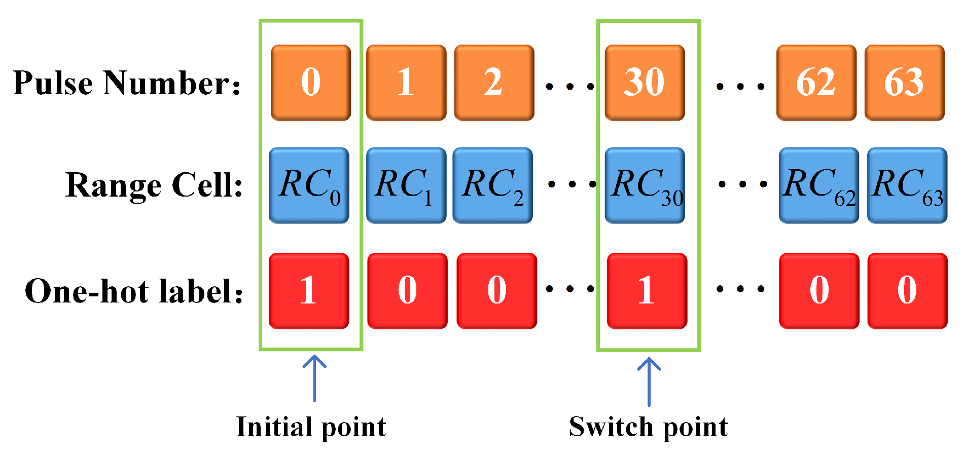
Figure 1 provides a more intuitive illustration of the above process. Assuming the number of pulses is $M=64$; the red boxes in the figure denote the labels of the initial point and switch point (marked as 1), while all other positions are labeled as 0. The training set $\Omega$ mainly consists of two parts: the radar echo signals $E\in {\mathbb{R}}^{2\times (2\times D+1)\times M}$ and the labels of keypoints $K_{d,m}$ (i.e.,the initial point and switch point), and d represents the range cell corresponding to the m-th pulse number. If there are Q groups of training samples, the dataset $\Omega$ can be expressed as follows:

$$\begin{array}{c}\hfill \Omega ={\left\{\left(E^q,K_{d,m}^q\right)\right\}}_{q=1,2,\dots ,Q}\end{array}$$

(15)

where the trajectory labels $K_{d,m}$ are formulated in a one-hot encoding format:

$$\begin{array}{c}\hfill \left\{\begin{array}{cc}{K}_{d,m}^q=1,& m=0,\gamma \\ K_{d,m}^q=0,& \mathrm{others}.\end{array}\right.\end{array}$$

(16)

where $\gamma$ denotes the pulse number corresponding to the mode-switching time.

When $E^q$ is the input of the network, the output is:

$$\begin{array}{c}\hfill {\widehat{K}}_{d,m}^q=\mathrm{Network}\left(E^q;w\right)\end{array}$$

(17)

where $w=\left[w_1,w_2,\dots ,w_{N_w}\right]$ represents the trainable hyperparameters of the network, and $N_w$ denotes the number of weights.

3.2. Architecture of the KDNet

In this section, a hierarchical residual network, referred to as the Keypoint Detection Network (KDNet), is proposed to detect two types of keypoints, i.e., the initial point and the switch point. The network mainly consists of two components: a hierarchical shrinking module (hsm) and a residual module (rm). The hierarchical shrinking module is designed to progressively reduce the resolution of the feature maps derived from the original radar echo signals while preserving key information from different receptive fields. This module is implemented by applying large convolutional kernels of various scales to perform down-sampling, thereby retaining as much feature information as possible. It serves as an essential component for feature compression and dimensionality reduction. For the residual module, its purpose is to deepen the network and extract more high-level features, while effectively preventing gradient vanishing or explosion. This module is implemented through multiple skip connections, enabling feature information to be transmitted to deeper layers without distortion.

The input size of data is $2\times \left(2\times D+1\right)\times M$, where the first term “2” represents the real and imaginary parts of the radar echo signal. When the radar echo data $E^q$ is fed into the hierarchical shrinking module, the output $h_{\mathrm{hsm}}$ is obtained by convolving the input with two different large-scale convolution kernels, $C_1=(14,7,32)$ and $C_2=(13,7,32)$. The number of channels in each convolutional layer of this module is 32. To represent the above computation process, we first define:

$$\begin{array}{c}\hfill f_{\mathrm{CBL},1}\left(\cdot \right)=f_{\mathrm{LR}}\left(f_{\mathrm{BN}}\left(C_1\left(\cdot \right)\right)\right)\end{array}$$

(18)

$$\begin{array}{c}\hfill f_{\mathrm{CBL},2}\left(\cdot \right)=f_{\mathrm{LR}}\left(f_{\mathrm{BN}}\left(C_2\left(\cdot \right)\right)\right)\end{array}$$

(19)

where $f_{\mathrm{BN}}$ denotes the batch normalization operation and $f_{\mathrm{LR}}$ represents the LeakyReLU activation function. Then, the output of the hierarchical shrinking module $h_{\mathrm{hsm}}$ is as follows:

$$\begin{array}{c}\hfill h_{\mathrm{hsm}}=f_{\mathrm{CBL},2}\left(f_{\mathrm{CBL},2}\left(f_{\mathrm{CBL},1}\left(f_{\mathrm{CBL},1}\left(E^q\right)\right)\right)\right).\end{array}$$

(20)

The structural parameters of the hierarchical shrinking module is shown in

Table 2. The structural parameters of the hierarchical shrinking module.

Module	Kernel Size	Channel	Stride	Padding
$C_1$	(14, 7)	32	(1, 1)	(0, 3)
$C_1$	(14, 7)	32	(1, 1)	(0, 3)
$C_2$	(13, 7)	32	(1, 1)	(0, 3)
$C_2$	(13, 7)	32	(1, 1)	(0, 3)

.

The residual module consists of three submodules, where the input is the output of hierarchical shrinking module $h_{\mathrm{hsm}}$, and the output of the residual module is $h_{\mathrm{rm}}$. We can also define:

$$\begin{array}{c}\hfill f_{\mathrm{CBL},3}^i\left(\cdot \right)=f_{\mathrm{LR}}\left(f_{\mathrm{BN}}\left(C_3^i\left(\cdot \right)\right)\right)\end{array}$$

(21)

$$\begin{array}{c}\hfill f_{\mathrm{CBL},4}^i\left(\cdot \right)=f_{\mathrm{LR}}\left(f_{\mathrm{BN}}\left(C_4^i\left(\cdot \right)\right)\right)\end{array}$$

(22)

where $C_3^i=(1,1,C_{out,i}),i=1,2,3$ and $C_4^i=(13,7,C_{out,i}),i=1,2,3$. It is noticed that the skip connections are implemented via $C_3^i$. The number of channels in each submodule are $C_{out,1}=64$, $C_{out,2}=82$ and $C_{out,3}=101$, respectively. Take the first residual submodule $h_{\mathrm{R},1}$ as an example, which can be expressed as follows:

$$\begin{array}{c}\hfill h_{\Delta \mathrm{R},1}=f_{\mathrm{CBL},3}^1\left(h_{\mathrm{hsm}}\right)+f_{\mathrm{CBL},4}^1\left(h_{\mathrm{hsm}}\right)\end{array}$$

(23)

$$\begin{array}{c}\hfill h_{\mathrm{R},1}=h_{\Delta \mathrm{R},1}+f_{\mathrm{CBL},4}^1\left(f_{\mathrm{CBL},4}^1\left(h_{\Delta \mathrm{R},1}\right)\right).\end{array}$$

(24)

Similarly, the second residual submodule $h_{\mathrm{R},2}$ is

$$\begin{array}{c}\hfill h_{\Delta \mathrm{R},2}=f_{\mathrm{CBL},3}^2\left(h_{\mathrm{R},1}\right)+f_{\mathrm{CBL},4}^2\left(h_{\mathrm{R},1}\right)\end{array}$$

(25)

$$\begin{array}{c}\hfill h_{\mathrm{R},2}=h_{\Delta \mathrm{R},2}+f_{\mathrm{CBL},4}^2\left(f_{\mathrm{CBL},4}^2\left(h_{\Delta \mathrm{R},2}\right)\right).\end{array}$$

(26)

The third residual submodule (the output of residual module) $h_{\mathrm{rm}}$ can be expressed as follows:

$$\begin{array}{c}\hfill h_{\Delta \mathrm{R},3}=f_{\mathrm{CBL},3}^3\left(h_{\mathrm{R},2}\right)+f_{\mathrm{CBL},4}^3\left(h_{\mathrm{R},2}\right)\end{array}$$

(27)

$$\begin{array}{c}\hfill h_{\mathrm{rm}}=h_{\Delta \mathrm{R},3}+f_{\mathrm{CBL},4}^3\left(f_{\mathrm{CBL},4}^3\left(h_{\Delta \mathrm{R},3}\right)\right).\end{array}$$

(28)

Finally, the convolutional kernel $C_5=\left(7,7,101\right)$ is employed to produce the probability maps $h_{\mathrm{keypoint}}$ corresponding to the initial point and the switch point, which can be expressed as follows:

$$\begin{array}{c}\hfill h_{\mathrm{keypoint}}=f_{\mathrm{sigmoid}}\left(f_{\mathrm{LR}}\left(f_{\mathrm{BN}}\left(C_5\left(h_{\mathrm{rm}}\right)\right)\right)\right)\end{array}$$

(29)

where $f_{\mathrm{sigmoid}}$ denotes the sigmoid function. The structural parameters of the residual module and the network output are listed in

Table 3. The structural parameters of the residual module and the network output.

Module	Kernel Size	Channel	Stride	Padding
$C_3^1$	(1, 1)	64	(2, 1)	(0, 0)
$C_4^1$	(13, 7)	64	(2, 1)	(6, 3)
$C_4^1$	(13, 7)	64	(1, 1)	(6, 3)
$C_4^1$	(13, 7)	64	(1, 1)	(6, 3)
$C_4^1$	(13, 7)	64	(1, 1)	(6, 3)
$C_3^2$	(1, 1)	82	(2, 1)	(0, 0)
$C_4^2$	(13, 7)	82	(2, 1)	(6, 3)
$C_4^2$	(13, 7)	82	(1, 1)	(6, 3)
$C_4^2$	(13, 7)	82	(1, 1)	(6, 3)
$C_4^2$	(13, 7)	82	(1, 1)	(6, 3)
$C_3^3$	(1, 1)	101	(2, 1)	(0, 0)
$C_4^3$	(13, 7)	101	(2, 1)	(6, 3)
$C_4^3$	(13, 7)	101	(1, 1)	(6, 3)
$C_4^3$	(13, 7)	101	(1, 1)	(6, 3)
$C_4^3$	(13, 7)	101	(1, 1)	(6, 3)
$C_5$	(7, 7)	101	(1, 1)	(0, 3)

.

3.3. Loss Function

Since one target trajectory contains only two keypoints, i.e., the initial point and the switch point, whereas the number non-keypoint samples overwhelmingly exceeds that of the keypoints, the datasets suffers from a serve class imbalance. Under such conditions, the conventional cross entropy loss tends to cause the network to overfit background noise and fail to effectively learn the discriminative features associate with keypoints.

To address the above issue and effectively supervise the feature learning around keypoint regions, a joint supervision loss function is developed. This strategy encourages the network to concentrate more on the features near the keypoints and on improving the detection accuracy. From the perspectives of keypoint classification and regression, the loss function is composed of two components: the Position-Aware Weighted Binary Cross-Entropy (PAW-BCE) loss and the Wing loss. The PAW-BCE loss is designed to distinguish the keypoints of the target trajectory from the background noise in radar echo signals. Specifically, it assigns higher weights to spatial positions corresponding to keypoints, thereby guiding the network to focus on these critical regions and enhancing the classification accuracy of keypoints. The PAW-BCE loss for a batch of data can be defined as follows:

$$\begin{array}{cc}{\mathcal{L}}_{\mathrm{PAW}-\mathrm{BCE}}=\hfill & -{\displaystyle \frac{W_{d,m}^q}{Q\times M\times (2\times D+1)}}\hfill \\ & \hfill \left(\sum _{q=1}^Q\sum _{d=1}^{2\times D+1}\sum _{m=0}^{M-1}{K}_{d,m}^q\log \left({\widehat{K}}_{d,m}^q\right)+\left(1-K_{d,m}^q\right)\log \left(1-{\widehat{K}}_{d,m}^q\right)\right)\end{array}$$

(30)

where $W_{d,m}^q$ denotes the position-aware weighted coefficients designed to enhance the significance of initial point and switch point, which is as follows:

$$\begin{array}{c}\hfill W_{d,m}^q=\left\{\begin{array}{cc}{\epsilon }_{{\mathrm{R}}_0},& (d,m)=\mathrm{initial}\mathrm{point}\\ {\epsilon }_{\mathrm{SP}},& (d,m)=\mathrm{switch}\mathrm{point}\\ 1,& \mathrm{others}.\end{array}\right.\end{array}$$

(31)

Since the variation range of the switch point in the range–pulse domain is larger than that of the initial point (as the anchor center of the sliding detection window is located at the initial point), the weight value at the switch point can be further increased, i.e., ${\epsilon }_{\mathrm{SP}}>{\epsilon }_{{\mathrm{R}}_0}$ so that the network pays more attention to the characteristic features around the switching point. As for the regression of keypoints, it is implemented using the Wing loss function, which is defined as follows:

$$\begin{array}{c}\hfill {\mathcal{L}}_{\mathrm{Wing}}\left(\delta \right)=\left\{\begin{array}{cc}\kappa ·\log \left(1+{\displaystyle \frac{\left|\delta \right|}{\varpi }}\right),& \left|\delta \right|<\kappa \\ \left|\delta \right|-Cons,& \mathrm{others}\end{array}\right.\end{array}$$

(32)

where $Cons=\kappa -\kappa ·\log \left(1+{\displaystyle \frac{\kappa }{\varpi }}\right)$ enforces continuity of the loss at the switching boundary precludes gradient discontinuities, $\varpi$ is a smoothing term for the logarithmic part that tempers the influence of small errors, $\kappa$ tunes the extent of the nonlinear segment, and $\delta$ represents the estimation residual. Overall, the loss function is:

$$\begin{array}{c}\hfill \mathcal{L}={\mathcal{L}}_{\mathrm{PAW}-\mathrm{BCE}}+\xi {\mathcal{L}}_{\mathrm{Wing}}\end{array}$$

(33)

where $\xi$ denotes the weight coefficient of the loss function. The weight parameter $\lambda$ was determined through empirical analysis. We observed that the model performance remains stable and insensitive to variations in $\xi$ within the range of $[0.5,1]$. In this work, we set $\xi =0.8$ to balance the loss terms.

3.4. Parameter Estimation

Based on the above method, the initial points and switch points can be obtained. Subsequently, energy accumulation is performed according to different motion phases, each corresponding to a specific precise range-evolution model. This section mainly discusses the coherent accumulation processes for four types of target motion: CVCA, CACV, CTCA, and CACT motion cases. For brevity and to avoid redundancy, only the procedures of parameter estimation for Case 1 (CVCA) and Case 3 (CTCA) are presented, as the remaining two (Case 2 and Case 4) can be derived in a similar manner to the above cases.

Case 1: According to Equation (10), the coherent integration method based on the CVCA motion target trajectory is as follows:

$$\begin{array}{cc}\hfill & r_{\mathrm{CVCA}}^s\left(t_m;{\dot{r}}_{\mathrm{CV},0}^s,v_{\mathrm{CV},0}^s,v_{\mathrm{CA},t_{\gamma }}^s,a_{\mathrm{CA},t_{\gamma }}^s,{\theta }_{va,t_{\gamma }}^s,{\theta }_{\dot{r}v,t_{\gamma }}^s\right)\hfill \\ \hfill & =\left\{\begin{array}{cc}\sqrt{r_{\mathrm{CV},0}^2+2r_{\mathrm{CV},0}{v}_{\mathrm{CV},0}^s\cos {\theta }_{\dot{r}v,0}^s{t}_m+{\left(v_{\mathrm{CV},0}^s\right)}^2{t}_m^2},& 0\le t_m\le t_{\gamma }\\ \sqrt{\begin{array}{c}{r}_{\mathrm{CA},t_{\gamma }}^2+2r_{\mathrm{CA},t_{\gamma }}{v}_{\mathrm{CA},t_{\gamma }}^s\cos {\theta }_{\dot{r}v,t_{\gamma }}^s{t}_m\hfill \\ +\left({\left(v_{\mathrm{CA},t_{\gamma }}^s\right)}^2+a_{\mathrm{CA},t_{\gamma }}^s{r}_{\mathrm{CA},t_{\gamma }}\cos {\theta }_{va,t_{\gamma }}^s\cos {\theta }_{\dot{r}v,t_{\gamma }}^s\right)t_m^2\hfill \\ +\cos {\theta }_{va,t_{\gamma }}^s{v}_{\mathrm{CA},t_{\gamma }}^s{a}_{\mathrm{CA},t_{\gamma }}^s{t}_m^3+0.25{\left(a_{\mathrm{CA},t_{\gamma }}^s\right)}^2{t}_m^4\hfill \end{array}},& t_{\gamma }<t_m\le t_{M-1}\end{array}\right.\hfill \end{array}$$

(34)

where ${\dot{r}}_{\mathrm{CV},0}^s,v_{\mathrm{CV},0}^s,v_{\mathrm{CA},t_{\gamma }}^s,a_{\mathrm{CA},t_{\gamma }}^s,{\theta }_{va,t_{\gamma }}^s,{\theta }_{\dot{r}v,t_{\gamma }}^s$ are the parameters to be searched, which are denoted with the superscript “s”.

According to (3) and (34), we can obtain the following:

$$\begin{array}{cc}\hfill & G\left({\dot{r}}_{\mathrm{CV},0}^s,v_{\mathrm{CV},0}^s,v_{\mathrm{CA},t_{\gamma }}^s,a_{\mathrm{CA},t_{\gamma }}^s,{\theta }_{va,t_{\gamma }}^s,{\theta }_{\dot{r}v,t_{\gamma }}^s\right)\hfill \\ \hfill =& \underset{0}{\overset{T}{\int }}{A}_{\mathrm{cs}}\mathrm{sinc}\left[B\left({\displaystyle \frac{2\left(r_{\mathrm{CVCA}}^s\left(t_m\right)-r_{\mathrm{CVCA}}\left(t_m\right)\right)}{c}}\right)\right]\times \exp \left[j4\pi {\displaystyle \frac{r_{\mathrm{CVCA}}^s\left(t_m\right)-r_{\mathrm{CVCA}}\left(t_m\right)}{\lambda }}\right]d{t}_m.\hfill \end{array}$$

(35)

When the search parameters match the true target parameters, i.e., ${\dot{r}}_{\mathrm{CV},0}^s={\dot{r}}_{\mathrm{CV},0},v_{\mathrm{CV},0}^s=v_{\mathrm{CV},0},v_{\mathrm{CA},t_{\gamma }}^s=v_{\mathrm{CA},t_{\gamma }},a_{\mathrm{CA},t_{\gamma }}^s=a_{\mathrm{CA},t_{\gamma }},{\theta }_{va,t_{\gamma }}^s={\theta }_{va,t_{\gamma }},{\theta }_{\dot{r}v,t_{\gamma }}^s={\theta }_{\dot{r}v,t_{\gamma }}$; we have the following:

$$r_{\mathrm{CVCA}}^s\left(t_m;{\dot{r}}_{\mathrm{CV},0}^s,v_{\mathrm{CV},0}^s,v_{\mathrm{CA},t_{\gamma }}^s,a_{\mathrm{CA},t_{\gamma }}^s,{\theta }_{va,t_{\gamma }}^s,{\theta }_{\dot{r}v,t_{\gamma }}^s\right)-r_{\mathrm{CVCA}}\left(t_m\right)\equiv 0.$$

(36)

The integration peak obtained during the accumulation process can be expressed as follows:

$$\begin{array}{cc}\hfill G\left({\dot{r}}_{\mathrm{CV},0}^s,v_{\mathrm{CV},0}^s,v_{\mathrm{CA},t_{\gamma }}^s,a_{\mathrm{CA},t_{\gamma }}^s,{\theta }_{va,t_{\gamma }}^s,{\theta }_{\dot{r}v,t_{\gamma }}^s\right)& =\underset{0}{\overset{T}{\int }}{A}_{\mathrm{cs}}\mathrm{sinc}\left({\displaystyle \frac{2B}{c}}\times 0\right)\times \exp \left(j{\displaystyle \frac{4\pi }{\lambda }}\times 0\right)d{t}_m\hfill \\ \hfill & =A_{\mathrm{cs}}T.\hfill \end{array}$$

(37)

It is noteworthy that prior to the matching process, the value ranges of the seven parameters involved in the CVCA target must be determined based on prior information. Specifically:

$$\begin{array}{c}\hfill {\dot{r}}_{\mathrm{CV},0}^s\left(n_{\mathrm{CV},0}^{\dot{r}}\right)={\dot{r}}_{\mathrm{CV},0}^{min}+n_{\mathrm{CV},0}^{\dot{r}}\Delta {\dot{r}}_{\mathrm{CV},0}\in \left[{\dot{r}}_{\mathrm{CV},0}^{min},{\dot{r}}_{\mathrm{CV},0}^{max}\right],n_{\mathrm{CV},0}^{\dot{r}}=0,1,\dots ,N_{\mathrm{CV},0}^{\dot{r}}-1\end{array}$$

(38)

$$\begin{array}{c}\hfill v_{\mathrm{CV},0}^s\left(n_{\mathrm{CV},0}^v\right)=v_{\mathrm{CV},0}^{min}+n_{\mathrm{CV},0}^v\Delta v_{\mathrm{CV},0}\in \left[v_{\mathrm{CV},0}^{min},v_{\mathrm{CV},0}^{max}\right],n_{\mathrm{CV},0}^v=0,1,\dots ,N_{\mathrm{CV},0}^v-1\end{array}$$

(39)

$$\begin{array}{c}\hfill v_{\mathrm{CA},t_{\gamma }}^s\left(n_{\mathrm{CA},t_{\gamma }}^v\right)=v_{\mathrm{CA},t_{\gamma }}^{min}+n_{\mathrm{CA},t_{\gamma }}^v\Delta v_{\mathrm{CA},t_{\gamma }}\in \left[v_{\mathrm{CA},t_{\gamma }}^{min},v_{\mathrm{CA},t_{\gamma }}^{max}\right],n_{\mathrm{CA},t_{\gamma }}^v=0,1,\dots ,N_{\mathrm{CA},t_{\gamma }}^v-1\end{array}$$

(40)

$$\begin{array}{c}\hfill a_{\mathrm{CA},t_{\gamma }}^s\left(n_{\mathrm{CA},t_{\gamma }}^a\right)=a_{\mathrm{CA},t_{\gamma }}^{min}+n_{\mathrm{CA},t_{\gamma }}^a\Delta a_{\mathrm{CA},t_{\gamma }}\in \left[a_{\mathrm{CA},t_{\gamma }}^{min},a_{\mathrm{CA},t_{\gamma }}^{max}\right],n_{\mathrm{CA},t_{\gamma }}^a=0,1,\dots ,N_{\mathrm{CA},t_{\gamma }}^a-1\end{array}$$

(41)

$$\begin{array}{c}\hfill {\theta }_{va,t_{\gamma }}^s\left(n_{\theta ,t_{\gamma }}^{va}\right)={\theta }_{va,t_{\gamma }}^{min}+n_{\theta ,t_{\gamma }}^{va}\Delta {\theta }_{va,t_{\gamma }}\in \left[{\theta }_{va,t_{\gamma }}^{min},{\theta }_{va,t_{\gamma }}^{max}\right],n_{\theta ,t_{\gamma }}^{va}=0,1,\dots ,N_{\theta ,t_{\gamma }}^{va}-1\end{array}$$

(42)

$$\begin{array}{c}\hfill {\theta }_{\dot{r}v,t_{\gamma }}^s\left(n_{\theta ,t_{\gamma }}^{\dot{r}v}\right)={\theta }_{\dot{r}v,t_{\gamma }}^{min}+n_{\theta ,t_{\gamma }}^{\dot{r}v}\Delta {\theta }_{\dot{r}v,t_{\gamma }}\in \left[{\theta }_{\dot{r}v,t_{\gamma }}^{min},{\theta }_{\dot{r}v,t_{\gamma }}^{max}\right],n_{\theta ,t_{\gamma }}^{\dot{r}v}=0,1,\dots ,N_{\theta ,t_{\gamma }}^{\dot{r}v}-1\end{array}$$

(43)

where $N_{\mathrm{CV},0}^{\dot{r}}$ and $N_{\mathrm{CV},0}^v$ denote the searching number of radial velocity and velocity in the CV phase, respectively. $N_{\mathrm{CA},t_{\gamma }}^v$, $N_{\mathrm{CA},t_{\gamma }}^a$, and $N_{\theta ,t_{\gamma }}^{\dot{r}v}$ denote the searching number of radial velocity, velocity, acceleration, the angle between velocity and acceleration, and the angle between radial velocity and velocity, respectively. Additionally, $\left[{\dot{r}}_{\mathrm{CV},0}^{min},{\dot{r}}_{\mathrm{CV},0}^{max}\right]$, $\left[v_{\mathrm{CV},0}^{min},v_{\mathrm{CV},0}^{max}\right]$, $\left[v_{\mathrm{CA},t_{\gamma }}^{min},v_{\mathrm{CA},t_{\gamma }}^{max}\right]$, $\left[a_{\mathrm{CA},t_{\gamma }}^{min},a_{\mathrm{CA},t_{\gamma }}^{max}\right]$, $\left[{\theta }_{va,t_{\gamma }}^{min},{\theta }_{va,t_{\gamma }}^{max}\right]$ and $\left[{\theta }_{\dot{r}v,t_{\gamma }}^{min},{\theta }_{\dot{r}v,t_{\gamma }}^{max}\right]$ represent the search ranges, which can be derived from prior information such as the target’s fundamental physical properties and empirical knowledge. $\Delta {\dot{r}}_{\mathrm{CV},0}$, $\Delta v_{\mathrm{CV},0}$, $\Delta v_{\mathrm{CA},t_{\gamma }}$, $\Delta a_{\mathrm{CA},t_{\gamma }}$, $\Delta {\theta }_{va,t_{\gamma }}$, and $\Delta {\theta }_{\dot{r}v,t_{\gamma }}$ correspond to the search intervals.

By incorporating all the search parameters into the trajectory equation of CVCA motion, we obtain the following:

$$\begin{array}{cc}\hfill & r_{\mathrm{CVCA}}^s\left(\begin{array}{c}{t}_m;{\dot{r}}_{\mathrm{CV},0}^s\left(n_{\mathrm{CV},0}^{\dot{r}}\right),v_{\mathrm{CV},0}^s\left(n_{\mathrm{CV},0}^v\right),v_{\mathrm{CA},t_{\gamma }}^s\left(n_{\mathrm{CA},t_{\gamma }}^v\right),\hfill \\ a_{\mathrm{CA},t_{\gamma }}^s\left(n_{\mathrm{CA},t_{\gamma }}^a\right),{\theta }_{va,t_{\gamma }}^s\left(n_{\theta ,t_{\gamma }}^{va}\right),{\theta }_{\dot{r}v,t_{\gamma }}^s\left(n_{\theta ,t_{\gamma }}^{\dot{r}v}\right)\hfill \end{array}\right)\hfill \\ \hfill & =\left\{\begin{array}{cc}\sqrt{r_{\mathrm{CV},0}^2+2r_{\mathrm{CV},0}{\dot{r}}_{\mathrm{CV},0}^s\left(n_{\mathrm{CV},0}^{\dot{r}}\right)t_m+{\left(v_{\mathrm{CV},0}^s\left(n_{\mathrm{CV},0}^v\right)\right)}^2{t}_m^2},& 0\le t_m\le t_{\gamma }\\ \sqrt{\begin{array}{c}{r}_{\mathrm{CA},t_{\gamma }}^2+2r_{\mathrm{CA},t_{\gamma }}{v}_{\mathrm{CA},t_{\gamma }}^s\left(n_{\mathrm{CA},t_{\gamma }}^v\right)\cos {\theta }_{\dot{r}v,t_{\gamma }}^s\left(n_{\theta ,t_{\gamma }}^{\dot{r}v}\right)t_m\hfill \\ +\left(\begin{array}{c}{\left(v_{\mathrm{CA},t_{\gamma }}^s\left(n_{\mathrm{CA},t_{\gamma }}^v\right)\right)}^2+a_{\mathrm{CA},t_{\gamma }}^s\left(n_{\mathrm{CA},t_{\gamma }}^a\right)r_{\mathrm{CA},t_{\gamma }}\hfill \\ \times \cos {\theta }_{va,t_{\gamma }}^s\left(n_{\theta ,t_{\gamma }}^{va}\right)\cos {\theta }_{\dot{r}v,t_{\gamma }}^s\left(n_{\theta ,t_{\gamma }}^{\dot{r}v}\right)\hfill \end{array}\right)t_m^2\hfill \\ +\cos {\theta }_{va,t_{\gamma }}^s\left(n_{\theta ,t_{\gamma }}^{va}\right)v_{\mathrm{CA},t_{\gamma }}^s\left(n_{\mathrm{CA},t_{\gamma }}^v\right)a_{\mathrm{CA},t_{\gamma }}^s\left(n_{\mathrm{CA},t_{\gamma }}^a\right)t_m^3\hfill \\ +0.25{\left(a_{\mathrm{CA},t_{\gamma }}^s\left(n_{\mathrm{CA},t_{\gamma }}^a\right)\right)}^2{t}_m^4\hfill \end{array}},& t_{\gamma }<t_m\le t_{M-1}\end{array}\right.\hfill \end{array}$$

(44)

The coherent integration output with respect to different search parameters can be expressed as follows:

$$\begin{array}{cc}\hfill & G\left(\begin{array}{c}{\dot{r}}_{\mathrm{CV},0}^s\left(n_{\mathrm{CV},0}^{\dot{r}}\right),v_{\mathrm{CV},0}^s\left(n_{\mathrm{CV},0}^v\right),v_{\mathrm{CA},t_{\gamma }}^s\left(n_{\mathrm{CA},t_{\gamma }}^v\right),a_{\mathrm{CA},t_{\gamma }}^s\left(n_{\mathrm{CA},t_{\gamma }}^a\right),{\theta }_{va,t_{\gamma }}^s\left(n_{\theta ,t_{\gamma }}^{va}\right),{\theta }_{\dot{r}v,t_{\gamma }}^s\left(n_{\theta ,t_{\gamma }}^{\dot{r}v}\right)\hfill \end{array}\right)\hfill \\ \hfill & =\sum _{m=0}^{M-1}{S}_{\mathrm{cs}}\left(〈{\displaystyle \frac{r_{\mathrm{CVCA}}^s\left(m{T}_r\right)}{\Delta r}}〉,m\right)\times \exp \left(j4\pi {\displaystyle \frac{r_{\mathrm{CVCA}}^s\left(m{T}_r\right)}{\lambda }}\right)\hfill \end{array}$$

(45)

Case 3: According to Equation (12), the coherent integration method based on the CTCA motion target trajectory is as follows:

$$\begin{array}{cc}\hfill & r_{\mathrm{CTCA}}^s\left(t_m;{\dot{r}}_{\mathrm{CT},0}^s,{\omega }_{\mathrm{CT},0}^s,{\sigma }_{\mathrm{CT},0}^s,v_{\mathrm{CA},t_{\gamma }}^s,a_{\mathrm{CA},t_{\gamma }}^s,{\theta }_{va,t_{\gamma }}^s,{\theta }_{\dot{r}v,t_{\gamma }}^s\right)\hfill \\ \hfill & =\left\{\begin{array}{cc}\sqrt{r_{\mathrm{CT},0}^2+{\displaystyle \frac{2\sin {\omega }_{\mathrm{CT},0}^s{t}_m}{{\omega }_{\mathrm{CT},0}^s}}{r}_{\mathrm{CT},0}{\dot{r}}_{\mathrm{CT},0}^s+{\displaystyle \frac{2\left(1-\cos {\omega }_{\mathrm{CT},0}^s{t}_m\right)}{{\left({\omega }_{\mathrm{CT},0}^s\right)}^2}}{\sigma }_{\mathrm{CT},0}^s},& 0\le t_m\le t_{\gamma }\\ \sqrt{\begin{array}{c}{r}_{\mathrm{CA},t_{\gamma }}^2+2r_{\mathrm{CA},t_{\gamma }}{v}_{\mathrm{CA}}^s\cos {\theta }_{\dot{r}v}^s{t}_m\hfill \\ +\left({\left(v_{\mathrm{CA},t_{\gamma }}^s\right)}^2+a_{\mathrm{CA},t_{\gamma }}^s{r}_{\mathrm{CA},t_{\gamma }}\cos {\theta }_{va,t_{\gamma }}^s\cos {\theta }_{\dot{r}v,t_{\gamma }}^s\right)t_m^2\hfill \\ +\cos {\theta }_{va,t_{\gamma }}^s{v}_{\mathrm{CA},t_{\gamma }}^s{a}_{\mathrm{CA},t_{\gamma }}^s{t}_m^3+0.25{\left(a_{\mathrm{CA},t_{\gamma }}^s\right)}^2{t}_m^4\hfill \end{array}},& t_{\gamma }<t_m\le t_{M-1}\end{array}\right.\hfill \end{array}$$

(46)

where ${\dot{r}}_{\mathrm{CT},0}^s,{\omega }_{\mathrm{CT},0}^s,{\sigma }_{\mathrm{CT},0}^s,v_{\mathrm{CA},t_{\gamma }}^s,a_{\mathrm{CA},t_{\gamma }}^s,{\theta }_{va,t_{\gamma }}^s,$ and ${\theta }_{\dot{r}v,t_{\gamma }}^s$ are the parameters to be searched, which are denoted with the superscript “s”.

According to (3) and (46), we can obtain the following:

$$\begin{array}{cc}\hfill & G\left({\dot{r}}_{\mathrm{CT},0}^s,{\omega }_{\mathrm{CT},0}^s,{\sigma }_{\mathrm{CT},0}^s,v_{\mathrm{CA},t_{\gamma }}^s,a_{\mathrm{CA},t_{\gamma }}^s,{\theta }_{va,t_{\gamma }}^s,{\theta }_{\dot{r}v,t_{\gamma }}^s\right)\hfill \\ \hfill & =\underset{0}{\overset{T}{\int }}{A}_{\mathrm{cs}}\mathrm{sinc}\left[B\left({\displaystyle \frac{2\left(r_{\mathrm{CTCA}}^s\left(t_m\right)-r_{\mathrm{CTCA}}\left(t_m\right)\right)}{c}}\right)\right]\times \exp \left(j4\pi {\displaystyle \frac{r_{\mathrm{CTCA}}^s\left(t_m\right)-r_{\mathrm{CTCA}}\left(t_m\right)}{\lambda }}\right)d{t}_m.\hfill \end{array}$$

(47)

When the search parameters match the true target parameters, i.e., ${\dot{r}}_{\mathrm{CT},0}^s={\dot{r}}_{\mathrm{CT},0},{\omega }_{\mathrm{CT},0}^s={\omega }_{\mathrm{CT},0},{\sigma }_{\mathrm{CT},0}^s={\sigma }_{\mathrm{CT},0},v_{\mathrm{CA},t_{\gamma }}^s=v_{\mathrm{CA},t_{\gamma }},a_{\mathrm{CA},t_{\gamma }}^s=a_{\mathrm{CA},t_{\gamma }},{\theta }_{va,t_{\gamma }}^s={\theta }_{va,t_{\gamma }},{\theta }_{\dot{r}v,t_{\gamma }}^s={\theta }_{\dot{r}v,t_{\gamma }}$; we have the following:

$$r_{\mathrm{CTCA}}^s\left(t_m;{\dot{r}}_{\mathrm{CT},0}^s,{\omega }_{\mathrm{CT},0}^s,{\sigma }_{\mathrm{CT},0}^s,v_{\mathrm{CA},t_{\gamma }}^s,a_{\mathrm{CA},t_{\gamma }}^s,{\theta }_{va,t_{\gamma }}^s,{\theta }_{\dot{r}v,t_{\gamma }}^s\right)-r_{\mathrm{CTCA}}\left(t_m\right)\equiv 0.$$

(48)

The integration peak obtained during the accumulation process can be expressed as follows:

$$\begin{array}{cc}\hfill G\left({\dot{r}}_{\mathrm{CT},0}^s,{\omega }_{\mathrm{CT},0}^s,{\sigma }_{\mathrm{CT},0}^s,v_{\mathrm{CA},t_{\gamma }}^s,a_{\mathrm{CA},t_{\gamma }}^s,{\theta }_{va,t_{\gamma }}^s,{\theta }_{\dot{r}v,t_{\gamma }}^s\right)& =\underset{0}{\overset{T}{\int }}{A}_{\mathrm{cs}}\mathrm{sinc}\left({\displaystyle \frac{2B}{c}}\times 0\right)\times \exp \left(j{\displaystyle \frac{4\pi }{\lambda }}\times 0\right)d{t}_m\hfill \\ \hfill & =A_{\mathrm{cs}}T.\hfill \end{array}$$

(49)

It is noteworthy that prior to the matching process, the value ranges of the seven parameters involved in the CTCA target must be determined based on prior information. Specifically:

$${\dot{r}}_{\mathrm{CT},0}^s\left(n_{\mathrm{CT},0}^{\dot{r}}\right)={\dot{r}}_{\mathrm{CT},0}^{min}+n_{\mathrm{CT},0}^{\dot{r}}\Delta {\dot{r}}_{\mathrm{CT},0}\in \left[{\dot{r}}_{\mathrm{CT},0}^{min},{\dot{r}}_{\mathrm{CT},0}^{max}\right],n_{\mathrm{CT},0}^{\dot{r}}=0,1,\dots ,N_{\mathrm{CT},0}^{\dot{r}}-1$$

(50)

$${\omega }_{\mathrm{CT},0}^s\left(n_{\mathrm{CT},0}^{\omega }\right)={\omega }_{\mathrm{CT},0}^{min}+n_{\mathrm{CT},0}^{\omega }\Delta {\omega }_{\mathrm{CT},0}\in \left[{\omega }_{\mathrm{CT},0}^{min},{\omega }_{\mathrm{CT},0}^{max}\right],n_{\mathrm{CT},0}^{\omega }=0,1,\dots ,N_{\mathrm{CT},0}^{\omega }-1$$

(51)

$${\sigma }_{\mathrm{CT},0}^s\left(n_{\mathrm{CT},0}^{\sigma }\right)={\sigma }_{\mathrm{CT},0}^{min}+n_{\mathrm{CT},0}^{\sigma }\Delta {\sigma }_{\mathrm{CT},0}\in \left[{\sigma }_{\mathrm{CT},0}^{min},{\sigma }_{\mathrm{CT},0}^{max}\right],n_{\mathrm{CT},0}^{\sigma }=0,1,\dots ,N_{\mathrm{CT},0}^{\sigma }-1$$

(52)

$$v_{\mathrm{CA},t_{\gamma }}^s\left(n_{\mathrm{CA},t_{\gamma }}^v\right)=v_{\mathrm{CA},t_{\gamma }}^{min}+n_{\mathrm{CA},t_{\gamma }}^v\Delta v_{\mathrm{CA},t_{\gamma }}\in \left[v_{\mathrm{CA},t_{\gamma }}^{min},v_{\mathrm{CA},t_{\gamma }}^{max}\right],n_{\mathrm{CA},t_{\gamma }}^v=0,1,\dots ,N_{\mathrm{CA},t_{\gamma }}^v-1$$

(53)

$$a_{\mathrm{CA},t_{\gamma }}^s\left(n_{\mathrm{CA},t_{\gamma }}^a\right)=a_{\mathrm{CA},t_{\gamma }}^{min}+n_{\mathrm{CA},t_{\gamma }}^a\Delta a_{\mathrm{CA},t_{\gamma }}\in \left[a_{\mathrm{CA},t_{\gamma }}^{min},a_{\mathrm{CA},t_{\gamma }}^{max}\right],n_{\mathrm{CA},t_{\gamma }}^a=0,1,\dots ,N_{\mathrm{CA},t_{\gamma }}^a-1$$

(54)

$${\theta }_{va,t_{\gamma }}^s\left(n_{\theta ,t_{\gamma }}^{va}\right)={\theta }_{va,t_{\gamma }}^{min}+n_{\theta ,t_{\gamma }}^{va}\Delta {\theta }_{va,t_{\gamma }}\in \left[{\theta }_{va,t_{\gamma }}^{min},{\theta }_{va,t_{\gamma }}^{max}\right],n_{\theta ,t_{\gamma }}^{va}=0,1,\dots ,N_{\theta ,t_{\gamma }}^{va}-1$$

(55)

$${\theta }_{\dot{r}v,t_{\gamma }}^s\left(n_{\theta ,t_{\gamma }}^{\dot{r}v}\right)={\theta }_{\dot{r}v,t_{\gamma }}^{min}+n_{\theta ,t_{\gamma }}^{\dot{r}v}\Delta {\theta }_{\dot{r}v,t_{\gamma }}\in \left[{\theta }_{\dot{r}v,t_{\gamma }}^{min},{\theta }_{\dot{r}v,t_{\gamma }}^{max}\right],n_{\theta ,t_{\gamma }}^{\dot{r}v}=0,1,\dots ,N_{\theta ,t_{\gamma }}^{\dot{r}v}-1$$

(56)

where $N_{\mathrm{CT},0}^{\dot{r}}$, $N_{\mathrm{CT},0}^{\omega }$, and $N_{\mathrm{CT},0}^{\sigma }$ denote the searching number of radial velocity, turn rate, and pseudo velocity in the CT phase, respectively. $N_{\mathrm{CA},t_{\gamma }}^v$, $N_{\mathrm{CA},t_{\gamma }}^a$, $N_{\theta ,t_{\gamma }}^{va}$, and $N_{\theta ,t_{\gamma }}^{\dot{r}v}$ denote the searching number of radial velocity, velocity, acceleration, the angle between velocity and acceleration, and the angle between radial velocity and velocity in the CA phase, respectively. Additionally, $\left[{\dot{r}}_{\mathrm{CT},0}^{min},{\dot{r}}_{\mathrm{CT},0}^{max}\right]$, $\left[{\omega }_{\mathrm{CT},0}^{min},{\omega }_{\mathrm{CT},0}^{max}\right]$, $\left[{\sigma }_{\mathrm{CT},0}^{min},{\sigma }_{\mathrm{CT},0}^{max}\right]$, $\left[v_{\mathrm{CA},t_{\gamma }}^{min},v_{\mathrm{CA},t_{\gamma }}^{max}\right]$, $\left[a_{\mathrm{CA},t_{\gamma }}^{min},a_{\mathrm{CA},t_{\gamma }}^{max}\right]$, $\left[{\theta }_{va,t_{\gamma }}^{min},{\theta }_{va,t_{\gamma }}^{max}\right]$, and $\left[{\theta }_{\dot{r}v,t_{\gamma }}^{min},{\theta }_{\dot{r}v,t_{\gamma }}^{max}\right]$ represent the search ranges, which can be derived from prior information such as the target’s fundamental physical properties and empirical knowledge. $\Delta {\dot{r}}_{\mathrm{CT},0}$, $\Delta {\omega }_{\mathrm{CT},0}$, $\Delta {\sigma }_{\mathrm{CT},0}$, $\Delta v_{\mathrm{CA},t_{\gamma }}$, $\Delta a_{\mathrm{CA},t_{\gamma }}$, $\Delta {\theta }_{va,t_{\gamma }}$, and $\Delta {\theta }_{\dot{r}v,t_{\gamma }}$ correspond to the search intervals.

By incorporating all the search parameters into the trajectory equation of CTCA motion, we obtain the following:

$$\begin{array}{cc}\hfill & r_{\mathrm{CTCA}}^s\left(\begin{array}{c}{t}_m;{\dot{r}}_{\mathrm{CT},0}^s\left(n_{\mathrm{CT},0}^{\dot{r}}\right),{\omega }_{\mathrm{CT},0}^s\left(n_{\mathrm{CT},0}^{\omega }\right),{\sigma }_{\mathrm{CT},0}^s\left(n_{\mathrm{CT},0}^{\sigma }\right),v_{\mathrm{CA},t_{\gamma }}^s\left(n_{\mathrm{CA},t_{\gamma }}^v\right),\hfill \\ a_{\mathrm{CA},t_{\gamma }}^s\left(n_{\mathrm{CA},t_{\gamma }}^a\right),{\theta }_{va,t_{\gamma }}^s\left(n_{\theta ,t_{\gamma }}^{va}\right),{\theta }_{\dot{r}v,t_{\gamma }}^s\left(n_{\theta ,t_{\gamma }}^{\dot{r}v}\right)\hfill \end{array}\right)\hfill \\ \hfill & =\left\{\begin{array}{cc}\sqrt{\begin{array}{c}{r}_{\mathrm{CT},0}^2+{\displaystyle \frac{2\sin {\omega }_{\mathrm{CT},0}^s\left(n_{\mathrm{CT},0}^{\omega }\right)t_m}{{\omega }_{\mathrm{CT},0}^s\left(n_{\mathrm{CT},0}^{\omega }\right)}}{r}_{\mathrm{CT},0}{\dot{r}}_{\mathrm{CT},0}^s\left(n_{\mathrm{CT},0}^{\dot{r}}\right)\hfill \\ +{\displaystyle \frac{2\left(1-\cos {\omega }_{\mathrm{CT},0}^s\left(n_{\mathrm{CT},0}^{\omega }\right)t_m\right)}{{\left({\omega }_{\mathrm{CT},0}^s\left(n_{\mathrm{CT},0}^{\omega }\right)\right)}^2}}{\sigma }_{\mathrm{CT},0}^s\left(n_{\mathrm{CT},0}^{\sigma }\right)\hfill \end{array}},& 0\le t_m\le t_{\gamma }\\ \sqrt{\begin{array}{c}{r}_{\mathrm{CA},t_{\gamma }}^2+2r_{\mathrm{CA},t_{\gamma }}{v}_{\mathrm{CA},t_{\gamma }}^s\left(n_{\mathrm{CA},t_{\gamma }}^v\right)\cos {\theta }_{\dot{r}v,t_{\gamma }}^s\left(n_{\theta ,t_{\gamma }}^{\dot{r}v}\right)t_m\hfill \\ +\left(\begin{array}{c}{\left(v_{\mathrm{CA},t_{\gamma }}^s\left(n_{\mathrm{CA},t_{\gamma }}^v\right)\right)}^2+a_{\mathrm{CA},t_{\gamma }}^s\left(n_{\mathrm{CA},t_{\gamma }}^a\right)r_{\mathrm{CA},t_{\gamma }}\hfill \\ \times \cos {\theta }_{va,t_{\gamma }}^s\left(n_{\theta ,t_{\gamma }}^{va}\right)\cos {\theta }_{\dot{r}v,t_{\gamma }}^s\left(n_{\theta ,t_{\gamma }}^{\dot{r}v}\right)\hfill \end{array}\right)t_m^2\hfill \\ +\cos {\theta }_{va,t_{\gamma }}^s\left(n_{\theta ,t_{\gamma }}^{va}\right)v_{\mathrm{CA},t_{\gamma }}^s\left(n_{\mathrm{CA},t_{\gamma }}^v\right)a_{\mathrm{CA},t_{\gamma }}^s\left(n_{\mathrm{CA},t_{\gamma }}^a\right)t_m^3\hfill \\ +0.25{\left(a_{\mathrm{CA},t_{\gamma }}^s\left(n_{\mathrm{CA},t_{\gamma }}^a\right)\right)}^2{t}_m^4\hfill \end{array}},& t_{\gamma }<t_m\le t_{M-1}\end{array}\right.\hfill \end{array}$$

(57)

The coherent integration output with respect to different search parameters can be expressed as follows:

$$\begin{array}{cc}\hfill & G\left(\begin{array}{c}{\dot{r}}_{\mathrm{CT},0}^s\left(n_{\mathrm{CT},0}^{\dot{r}}\right),{\omega }_{\mathrm{CT},0}^s\left(n_{\mathrm{CT},0}^{\omega }\right),{\sigma }_{\mathrm{CT},0}^s\left(n_{\mathrm{CT},0}^{\sigma }\right),v_{\mathrm{CA},t_{\gamma }}^s\left(n_{\mathrm{CA},t_{\gamma }}^v\right),\hfill \\ a_{\mathrm{CA},t_{\gamma }}^s\left(n_{\mathrm{CA},t_{\gamma }}^a\right),{\theta }_{va,t_{\gamma }}^s\left(n_{\theta ,t_{\gamma }}^{va}\right),{\theta }_{\dot{r}v,t_{\gamma }}^s\left(n_{\theta ,t_{\gamma }}^{\dot{r}v}\right)\hfill \end{array}\right)\hfill \\ \hfill & =\sum _{m=0}^{M-1}{S}_{\mathrm{cs}}\left(〈{\displaystyle \frac{r_{\mathrm{CTCA}}^s\left(m{T}_r\right)}{\Delta r}}〉,m\right)\times \exp \left(j4\pi {\displaystyle \frac{r_{\mathrm{CTCA}}^s\left(m{T}_r\right)}{\lambda }}\right)\hfill \end{array}$$

(58)

The integration output matrices are first computed by iteratively evaluating all combinations of search parameters. Based on these results, target detection is subsequently carried out using a Constant False Alarm Rate (CFAR) method [33], which is:

$$\eta =\sqrt{2{\widehat{\sigma }}^2\ln \left({\displaystyle \frac{1}{P_{fa}}}\right)}$$

(59)

where $P_{fa}$ denotes the false alarm probability, $\widehat{\sigma }$ is the estimated noise power and can be written as:

$$\widehat{\sigma }=\sum _{i=1}^{N_c}{\displaystyle \frac{\left|x_i\right|}{N_c}}$$

(60)

where the echo signal of the ith range cell is $x_i$, and $N_c$ denotes the window length for noise power estimation. A target is declared present if the energy peak surpasses the predefined threshold; otherwise, it is deemed absent. This decision process can be mathematically formulated as:

$$\left|G\left(\cdot \right)\right|\underset{H_0}{\stackrel{H_1}{\gtrless }}\eta$$

(61)

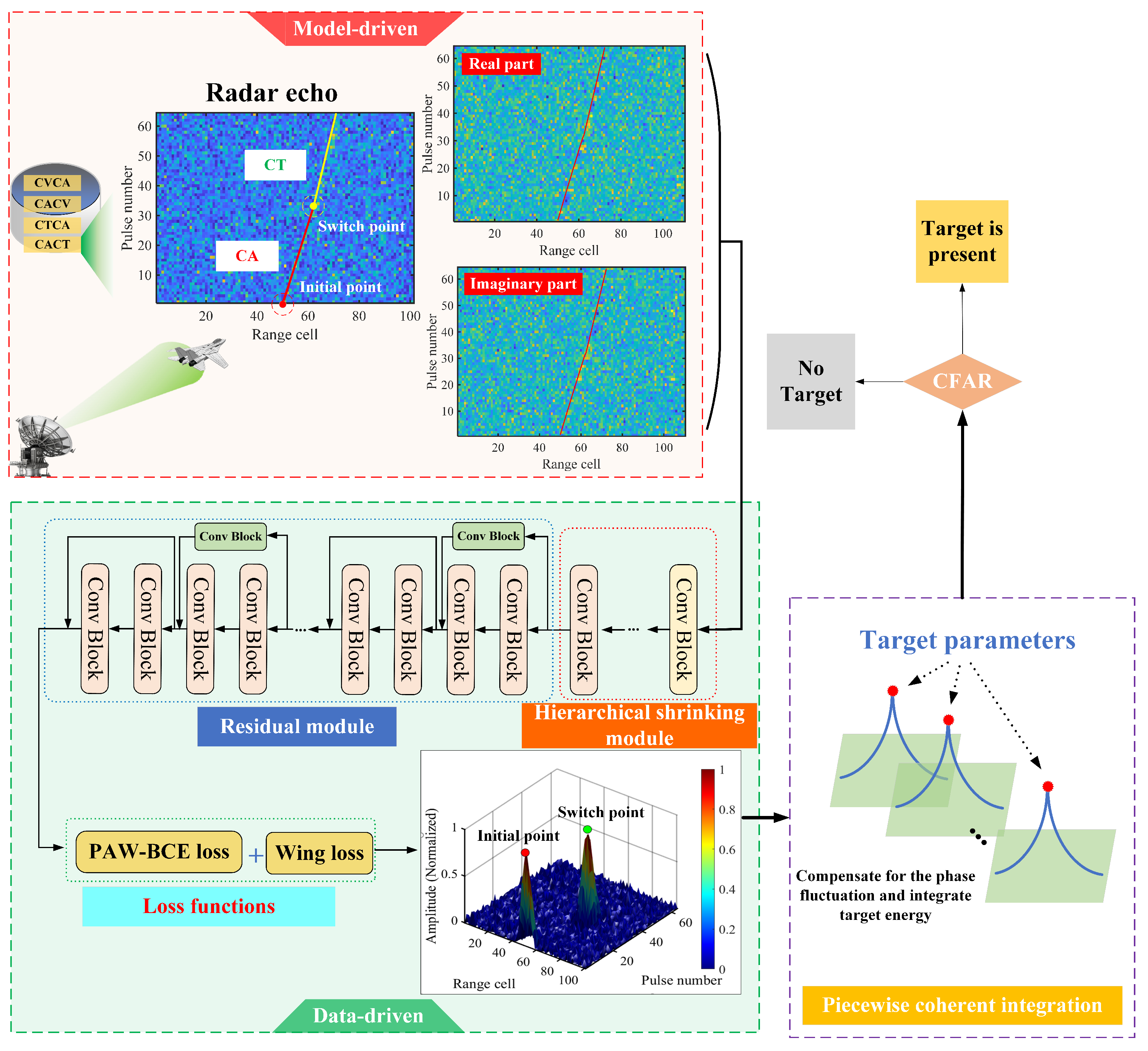
where $H_0$ represents the hypothesis of target absence, while represents the hypothesis of target presence. $H_1$ represents the energy accumulation in the four scenarios mentioned above. The overall structure of the proposed method is summarized in Figure 2.

3.5. Computational Cost

Floating-point operations (FLOPs) serve as an evaluation metric that directly reflects the computational efficiency of a network and are commonly used to measure its computational cost. Both the training and inference speeds of a network are affected by its computational complexity. The computational complexity of the proposed method in this paper arises from two aspects: the network part and the parameter estimation part. The first part is primarily determined by factors such as the convolutional kernel size, number of channels, padding, etc., which can be expressed as:

$$\begin{array}{cc}\hfill & \mathrm{FLOP}{\mathrm{s}}_{\mathrm{KDNet}}=\hfill \\ \hfill & \left({\displaystyle \frac{2C_{out}^l\left(C_{in}^l{S}_h^l{S}_w^l+1\right)}{{\displaystyle \prod _{i=1}^l}{S}_w^i}}\times \left({\displaystyle \frac{1}{{\displaystyle \prod _{i=1}^l}{S}_h^i}}\left(\begin{array}{c}M+\sum _{p=1}^{l-1}\prod _{q=1}^p{S}_h^q-\sum _{p=1}^l{K}_h^p\prod _{q=0}^{p-1}{S}_h^q\hfill \\ +2\times \sum _{p=1}^l{P}_h^p\prod _{q=0}^{p-1}{S}_h^q\hfill \end{array}\right)+1\right)\right)\times N_r\hfill \\ \hfill & +\left(\begin{array}{c}2C_{out}^l\left(C_{in}^l{S}_h^l{S}_w^l+1\right)\times \left({\displaystyle \frac{1}{{\displaystyle \prod _{i=1}^l}{S}_w^i}}\left(\begin{array}{c}\sum _{p=1}^{l-1}\prod _{q=1}^p{S}_w^q-\sum _{p=1}^l{K}_w^q\prod _{q=0}^{p-1}{S}_w^q\hfill \\ +2\times \sum _{p=1}^l{P}_w^q\prod _{q=0}^{p-1}{S}_w^q\hfill \end{array}\right)+1\right)\hfill \\ \times \left({\displaystyle \frac{1}{{\displaystyle \prod _{i=1}^l}{S}_h^i}}\left(\begin{array}{c}M+\sum _{p=1}^{l-1}\prod _{q=1}^p{S}_h^q-\sum _{p=1}^l{K}_h^q\prod _{q=0}^{p-1}{S}_h^q\hfill \\ +2\times \sum _{p=1}^l{P}_h^q\prod _{q=0}^{p-1}{S}_h^q\hfill \end{array}\right)+1\right)\hfill \end{array}\right)\hfill \\ \hfill & \end{array}$$

(62)

where L denotes the total number of layers. $C_{in}^l$ and $C_{out}^l$ indicate the numbers of input and output channels of the lth layer, respectively. $S_w^l$ and $S_h^l$ denote the stride along the width and height directions of the lth layer. $J_w^p$ and $J_h^p$ denote the width and height of the convolutional kernel at the $p\in \left[1,l-1\right]$th layer. $N_r$ represents the number of range cells.

The computational cost of the motion parameter estimation part depends on the motion model of the target trajectory. Specifically, for the CVCA and CACV motion cases, it can be expressed as follows:

$$\mathrm{FLOP}{\mathrm{s}}_{\mathrm{PE}\_\mathrm{CV}\_\mathrm{CA}}=N_{\mathrm{CV}}^{\dot{r}}{N}_{\mathrm{CV}}^v{N}_{\mathrm{CA}}^{\dot{r}}{N}_{\mathrm{CA}}^v{N}_{\mathrm{CA}}^a{N}_{\theta }^{va}{N}_{\theta }^{\dot{r}v}\left(8M-2\right)$$

(63)

Similarly, the computational complexity for the CTCA and CACT motion cases can be expressed as follows:

$$\mathrm{FLOP}{\mathrm{s}}_{\mathrm{PE}\_\mathrm{CT}\_\mathrm{CA}}=N_{\mathrm{CT}}^{\dot{r}}{N}_{\mathrm{CT}}^{\omega }{N}_{\mathrm{CT}}^{\sigma }{N}_{\mathrm{CA}}^{\dot{r}}{N}_{\mathrm{CA}}^v{N}_{\mathrm{CA}}^a{N}_{\theta }^{va}{N}_{\theta }^{\dot{r}v}\left(8M-2\right)$$

(64)

In summary, the computational complexity of the proposed algorithm can be expressed as follows:

$$\mathrm{FLOP}{\mathrm{s}}_{\mathrm{Network}\_\mathrm{CV}\_\mathrm{CA}}=\mathrm{FLOP}{\mathrm{s}}_{\mathrm{KDNet}}+\mathrm{FLOP}{\mathrm{s}}_{\mathrm{PE}\_\mathrm{CV}\_\mathrm{CA}}.$$

(65)

or:

$$\mathrm{FLOP}{\mathrm{s}}_{\mathrm{Network}\_\mathrm{CT}\_\mathrm{CA}}=\mathrm{FLOP}{\mathrm{s}}_{\mathrm{KDNet}}+\mathrm{FLOP}{\mathrm{s}}_{\mathrm{PE}\_\mathrm{CT}\_\mathrm{CA}}.$$

(66)

Several other coherent accumulation algorithms are introduced for comparison, namely GRFT [18], MTD [33], and FCN [24]. The FLOPs of the GRFT algorithm are given by:

$$\mathrm{FLOP}{\mathrm{s}}_{\mathrm{GRFT}\_\mathrm{CV}\_\mathrm{CA}}=N_{\mathrm{CV}}^r{N}_{\mathrm{CV}}^{\dot{r}}{N}_{\mathrm{CV}}^v{N}_{\mathrm{CA}}^r{N}_{\mathrm{CA}}^{\dot{r}}{N}_{\mathrm{CA}}^v{N}_{\mathrm{CA}}^a{N}_{\theta }^{va}{N}_{\theta }^{\dot{r}v}\left(8M-2\right)$$

(67)

or:

$$\mathrm{FLOP}{\mathrm{s}}_{\mathrm{GRFT}\_\mathrm{CT}\_\mathrm{CA}}=N_{\mathrm{CT}}^r{N}_{\mathrm{CT}}^{\dot{r}}{N}_{\mathrm{CT}}^{\omega }{N}_{\mathrm{CT}}^{\sigma }{N}_{\mathrm{CA}}^r{N}_{\mathrm{CA}}^{\dot{r}}{N}_{\mathrm{CA}}^v{N}_{\mathrm{CA}}^a{N}_{\theta }^{va}{N}_{\theta }^{\dot{r}v}\left(8M-2\right)$$

(68)

The FLOP of the MTD algorithm is:

$$\mathrm{FLOP}{\mathrm{s}}_{\mathrm{MTD}}=5M{N}_r{\log }_2\left(M\right)$$

(69)

The FLOP of the FCN is:

$$\mathrm{FLOP}{\mathrm{s}}_{\mathrm{FCN}}=k_{\mathrm{FCN}}{N}_r+b_{\mathrm{FCN}},k_{\mathrm{FCN}}=\sum _{l=1}^L{k}_{\mathrm{FCN}},b_{\mathrm{FCN}}=\sum _{l=1}^L{b}_{\mathrm{FCN}}.$$

(70)

4. Discussion of Simulation Results

In this section, multiple experiments and discussion are conducted to demonstrate the performance of the proposed method in terms of parameter estimation, detection probability, and computational complexity.

4.1. Parameter Settings

The radar system parameters are listed in

Table 4. Radar parameters.

Parameter	Values
Carrier frequency	3 GHz
Bandwidth	20 MHz
Sampling frequency	40 MHz
Pulse repetition frequency	200 Hz
Number of radar pulses	64

. As for the training process, the size of the training data is $2\times 101\times 64$.

Table 5. Training hyperparameters.

Parameter	Values
Learning rate	0.01
Batch size	40
Epoch	20

shows the training hyperparameters of network. The weighting coefficients, smoothing factors, and threshold are empirically determined through preliminary trials to ensure stable training and do not require further tuning across experiments. The switch point is ${\epsilon }_{\mathrm{SP}}=15$, the initial point is ${\epsilon }_{{\mathrm{R}}_0}=10$, and they satisfy ${\epsilon }_{\mathrm{SP}}>{\epsilon }_{{\mathrm{R}}_0}$. Meanwhile, the threshold is $\kappa =3$, and the smoothing factor of the logarithmic function is $\varpi =1$. To clarify the valid scope of the proposed method, we summarize the applicable boundary conditions in

Table 6. Target motion parameters.

Parameter	Values
Velocity	[−325 m/s, 325 m/s]
Acceleration	[−150 m/${\mathrm{s}}^2$, 150 m/${\mathrm{s}}^2$]
Turn rate	[−1 rad/s, 1 rad/s]
Switch point	[5th, 59th]
Target trajectory	4,000,000
SNR	[−3 dB, 6 dB]

. As shown in the table, the proposed method is effective under the conditions where the SNR ranges from −3 dB to 6 dB, and the target velocity and acceleration are within the ranges of [−325 m/s, 325 m/s] and [−150 m/${\mathrm{s}}^2$, 150 m/${\mathrm{s}}^2$], respectively. Regarding the number of targets, a sliding window detection scheme is employed to resolve multiple targets. These constraints ensure the reliable detection and parameter estimation of the targets.

It is worth noting that while this work focuses on single mode-switching scenarios, the proposed method can be extended to handle multiple motion state changes. By annotating multiple switching instants as key points in the training data, the network can learn to detect multiple transitions within a longer observation period, demonstrating the scalability of the proposed approach. Furthermore, although the training dataset in this work consists of CV, CA, and CT models, the proposed framework is applicable to non-constant motion. Due to the data-driven nature of the network, detecting complex maneuvers can be achieved by incorporating non-constant motion samples into the training set, allowing the model to learn the corresponding feature representations.

To evaluate the keypoint detection robustness across different SNRs, we define the detection accuracy for the initial point ($k=1$) and the switch point ($k=2$). Let ${\mathbf{p}}_{n,k}^{*}=(d_{n,k}^{*},m_{n,k}^{*})$ denote the ground truth position (range and pulse) in the n-th Monte Carlo trial, and let ${\widehat{\mathbf{p}}}_{n,k}=({\widehat{d}}_{n,k},{\widehat{m}}_{n,k})$ denote the estimated position. A detection is considered successful only if the estimated coordinates strictly match the ground truth. The accuracy for the k-th keypoint, denoted as ${\mathcal{A}}_k$, is calculated as:

$${\mathcal{A}}_k\left({\chi }_{\mathrm{SNR}}\right)={\displaystyle \frac{1}{N}}\sum _{n=1}^N\mathbb{I}\left({\widehat{\mathbf{p}}}_{n,k}={\mathbf{p}}_{n,k}^{*}\right),k\in \{1,2\}$$

(71)

where N is the total number of Monte Carlo trials, and $\mathbb{I}(·)$ is the indicator function, which equals 1 if the condition holds and 0 otherwise. ${\chi }_{\mathrm{SNR}}$ denotes the SNR after PC. Consequently, the average keypoint detection accuracy ${\mathcal{A}}_{\mathrm{avg}}$ is defined as follows:

$${\mathcal{A}}_{\mathrm{avg}}\left({\chi }_{\mathrm{SNR}}\right)={\displaystyle \frac{1}{2}}\left({\mathcal{A}}_1\left({\chi }_{\mathrm{SNR}}\right)+{\mathcal{A}}_2\left({\chi }_{\mathrm{SNR}}\right)\right).$$

(72)

4.2. Integration for Single Target

This section presents the integration performance tests for a single CVCA target, CACV target, CACT target, and CTCA target.

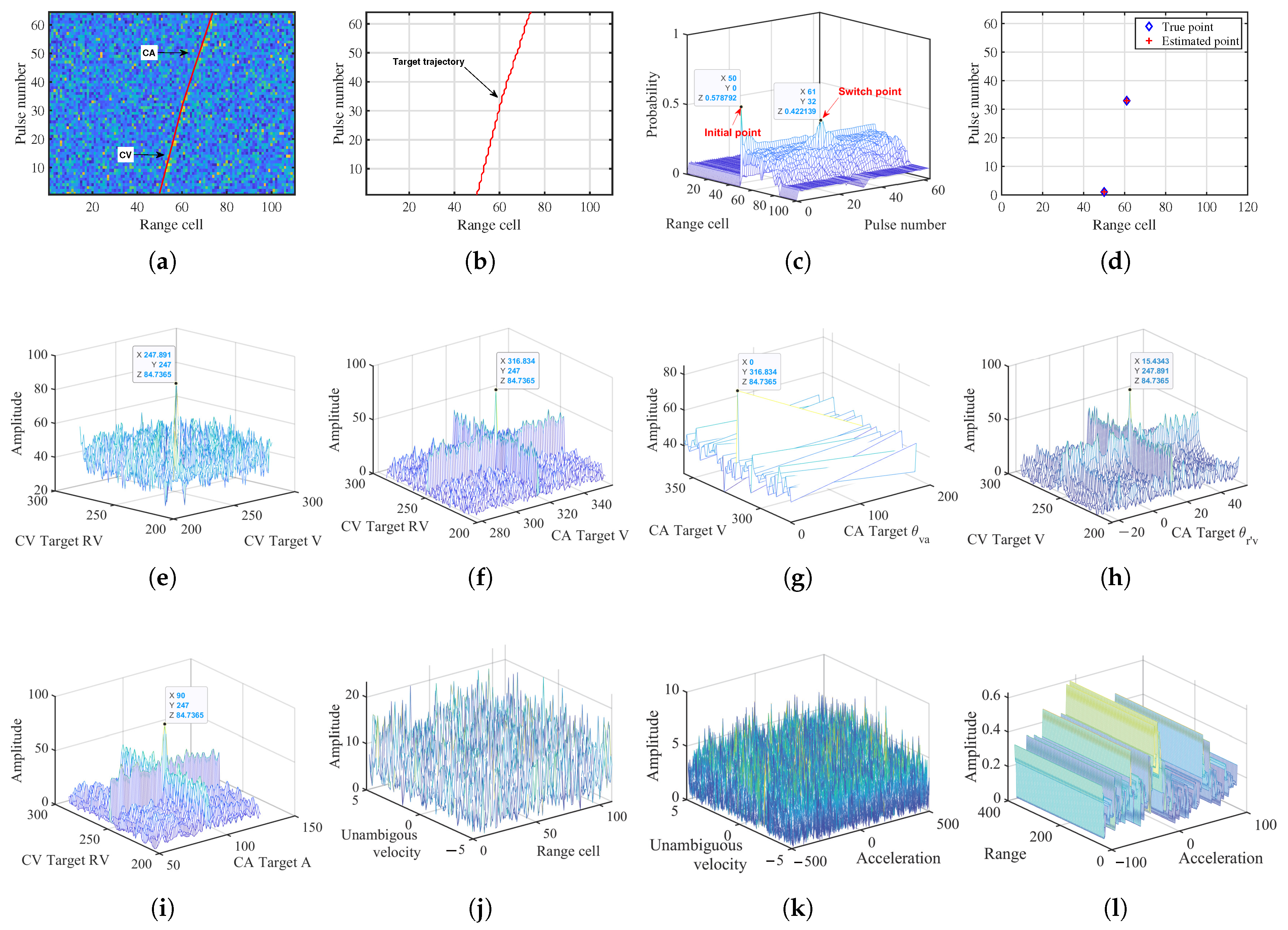
Case 1: In the CVCA motion scenario, the CVCA target’s motion parameters are as follows: the initial Cartesian position is $(p_{x,0}^{\mathrm{CV}},p_{y,0}^{\mathrm{CV}})=(112.5\mathrm{m},150\mathrm{m})$, the velocity of the target is $(v_x^{\mathrm{CV}},v_y^{\mathrm{CV}})=(165\mathrm{m}/\mathrm{s},185\mathrm{m}/\mathrm{s})$. When the motion mode switches from CV to CA, the velocity of the target is $(v_x^{\mathrm{CA}},v_y^{\mathrm{CA}})=(228\mathrm{m}/\mathrm{s},220\mathrm{m}/\mathrm{s})$, the acceleration of the target is $(a_x^{\mathrm{CA}},a_y^{\mathrm{CA}})=(72{\mathrm{m}/\mathrm{s}}^2,54{\mathrm{m}/\mathrm{s}}^2)$. The mode-switching occurs at the 32nd pulse. The SNR after PC is 2 dB. The true value of the target parameter is calculated to be $({\dot{r}}_{\mathrm{CV},0},v_{\mathrm{CV},0},v_{\mathrm{CA},t_{\gamma }},a_{\mathrm{CA},t_{\gamma }},{\theta }_{va,t_{\gamma }},{\theta }_{\dot{r}v,t_{\gamma }})$ = $(247\mathrm{m}/\mathrm{s},247.89\mathrm{m}/\mathrm{s},316.83\mathrm{m}/\mathrm{s},90{\mathrm{m}/\mathrm{s}}^2,0°,15.43°)$.

Figure 3a displays the pulse-compressed signal with a SNR of 2 dB. Figure 3b shows the target trajectory marked by a solid line. Figure 3c presents the probability heatmap generated by the KDNet output. Figure 3d shows the comparative result between the ground truth keypoints and the estimated keypoints. Figure 3e displays the estimated radial velocity ${\widehat{\dot{r}}}_{\mathrm{CV},0}$ and the estimated velocity ${\widehat{v}}_{\mathrm{CV},0}$ during the CV phase. Figure 3f shows the estimated radial velocity ${\widehat{\dot{r}}}_{\mathrm{CV},0}$ during the CV phase and the estimated velocity ${\widehat{v}}_{\mathrm{CA},t_{\gamma }}$ during the CA phase. Figure 3g displays the estimated velocity ${\widehat{v}}_{\mathrm{CA},t_{\gamma }}$ and the estimated angle ${\widehat{\theta }}_{va}$ during the CA phase. Figure 3h presents the estimated velocity ${\widehat{v}}_{\mathrm{CV},0}$ during the CV phase and the estimated angle ${\widehat{\theta }}_{\dot{r}v}$ during the CA phase. Figure 3i shows the estimated radial velocity ${\widehat{\dot{r}}}_{\mathrm{CV},0}$ during the CV phase and the estimated acceleration ${\widehat{a}}_{\mathrm{CA},t_{\gamma }}$ during the CA phase. Figure 3j displays the integration results of MTD. Figure 3k shows the integration results of FCN-dechirp. Figure 3l presents the integration results of third-order GRFT.

As illustrated in Figure 3e–i, the estimated target parameters are obtained as $({\widehat{\dot{r}}}_{\mathrm{CV},0},{\widehat{v}}_{\mathrm{CV},0},{\widehat{v}}_{\mathrm{CA},t_{\gamma }},{\widehat{a}}_{\mathrm{CA},t_{\gamma }},{\widehat{\theta }}_{va,t_{\gamma }},{\widehat{\theta }}_{\dot{r}v,t_{\gamma }})$ = $(247\mathrm{m}/\mathrm{s},247.89\mathrm{m}/\mathrm{s},316.83\mathrm{m}/\mathrm{s},90{\mathrm{m}/\mathrm{s}}^2,0°,$$15.43°)$. The results demonstrate that the proposed algorithm can accurately estimate both the initial point and the switch point, with parameter estimates closely approximating ground truth values.

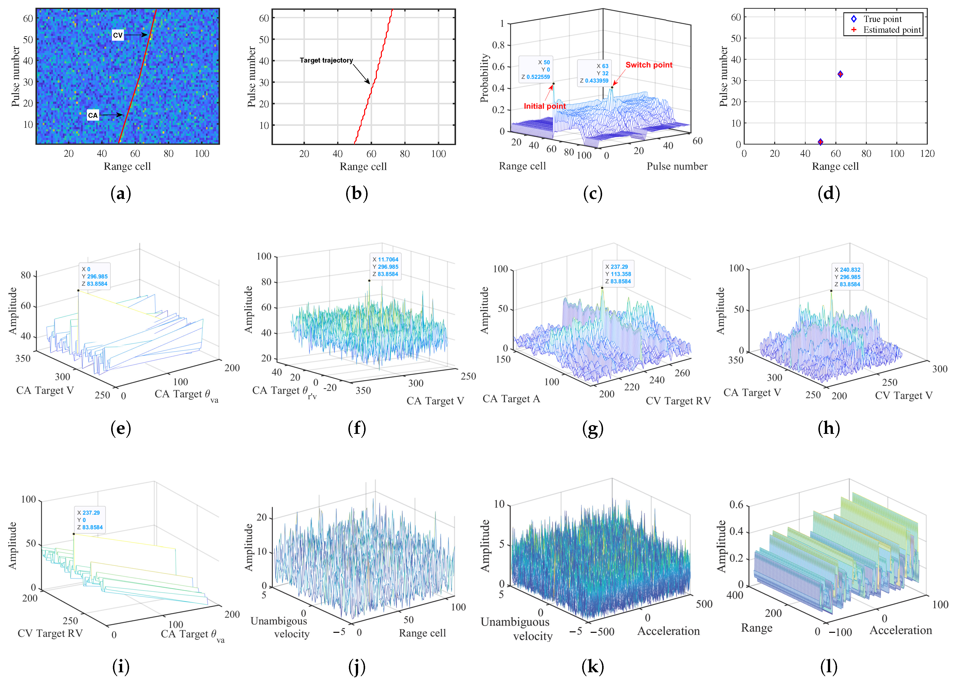
Case 2: In the CACV motion scenario, the CACV target’s motion parameters are as follows: the initial Cartesian position is $(p_{x,0}^{\mathrm{CA}},p_{y,0}^{\mathrm{CA}})=(112.5\mathrm{m},150\mathrm{m})$, the velocity of the target is $(v_x^{\mathrm{CA}},v_y^{\mathrm{CA}})=(210\mathrm{m}/\mathrm{s},210\mathrm{m}/\mathrm{s})$, the acceleration of the target is $(a_x^{\mathrm{CA}},a_y^{\mathrm{CA}})=(85{\mathrm{m}/\mathrm{s}}^2,75{\mathrm{m}/\mathrm{s}}^2)$. When the motion mode switches from CA to CV, the velocity of the target is $(v_x^{\mathrm{CV}},v_y^{\mathrm{CV}})=(180\mathrm{m}/\mathrm{s},160\mathrm{m}/\mathrm{s})$. The mode-switching occurs at the 32nd pulse. The SNR after PC is 2 dB. The true value of the target parameter is calculated to be $(v_{\mathrm{CA},0},a_{\mathrm{CA},0},{\theta }_{va,0},{\theta }_{\dot{r}v,0},{\dot{r}}_{\mathrm{CV},t_{\gamma }},v_{\mathrm{CV},t_{\gamma }})$ = $(296.99\mathrm{m}/\mathrm{s},113.36{\mathrm{m}/\mathrm{s}}^2,0°,11.71°,237.29\mathrm{m}/\mathrm{s},240.83\mathrm{m}/\mathrm{s})$.

Figure 4a displays the pulse-compressed signal with a SNR of 2 dB. Figure 4b shows the target trajectory marked by a solid line. Figure 4c presents the probability heatmap generated by the KDNet output. Figure 4d shows the comparative result between the ground truth keypoints and the estimated keypoints. Figure 4e displays the estimated velocity ${\widehat{v}}_{\mathrm{CA},0}$ and the estimated ${\widehat{\theta }}_{va}$ during the CA phase. Figure 4f presents the estimated velocity ${\widehat{v}}_{\mathrm{CA},0}$ and the estimated angle ${\widehat{\theta }}_{\dot{r}a}$ during the CA phase. Figure 4g shows the estimated acceleration ${\widehat{a}}_{\mathrm{CA},0}$ during the CA phase and the estimated radial velocity ${\widehat{\dot{r}}}_{\mathrm{CV},t_{\gamma }}$ during the CV phase. Figure 4h displays the estimated velocity ${\widehat{v}}_{\mathrm{CV},t_{\gamma }}$ during the CV phase and the estimated velocity ${\widehat{v}}_{\mathrm{CA},0}$ during the CA phase. Figure 4i shows the estimated radial velocity ${\widehat{\dot{r}}}_{\mathrm{CV},t_{\gamma }}$ during the CV phase and the estimated angle ${\widehat{\theta }}_{va}$ during the CA phase. Figure 4j displays the integration results of MTD. Figure 4k shows the integration results of FCN-dechirp. Figure 4l presents the integration results of third-order GRFT.

As illustrated in Figure 4e–i, the estimated target parameters are obtained as $({\widehat{v}}_{\mathrm{CA},0},{\widehat{a}}_{\mathrm{CA},0},{\widehat{\theta }}_{va,0},{\widehat{\theta }}_{\dot{r}v,0},{\widehat{\dot{r}}}_{\mathrm{CV},t_{\gamma }},{\widehat{v}}_{\mathrm{CV},t_{\gamma }})$ = $(296.99\mathrm{m}/\mathrm{s},113.36{\mathrm{m}/\mathrm{s}}^2,0°,11.71°,237.29\mathrm{m}/\mathrm{s}$, $240.83\mathrm{m}/\mathrm{s})$. The results indicate that the proposed algorithm achieves accurate estimation of both the initial and switch points, yielding parameter estimates that remain closely aligned with the ground-truth values.

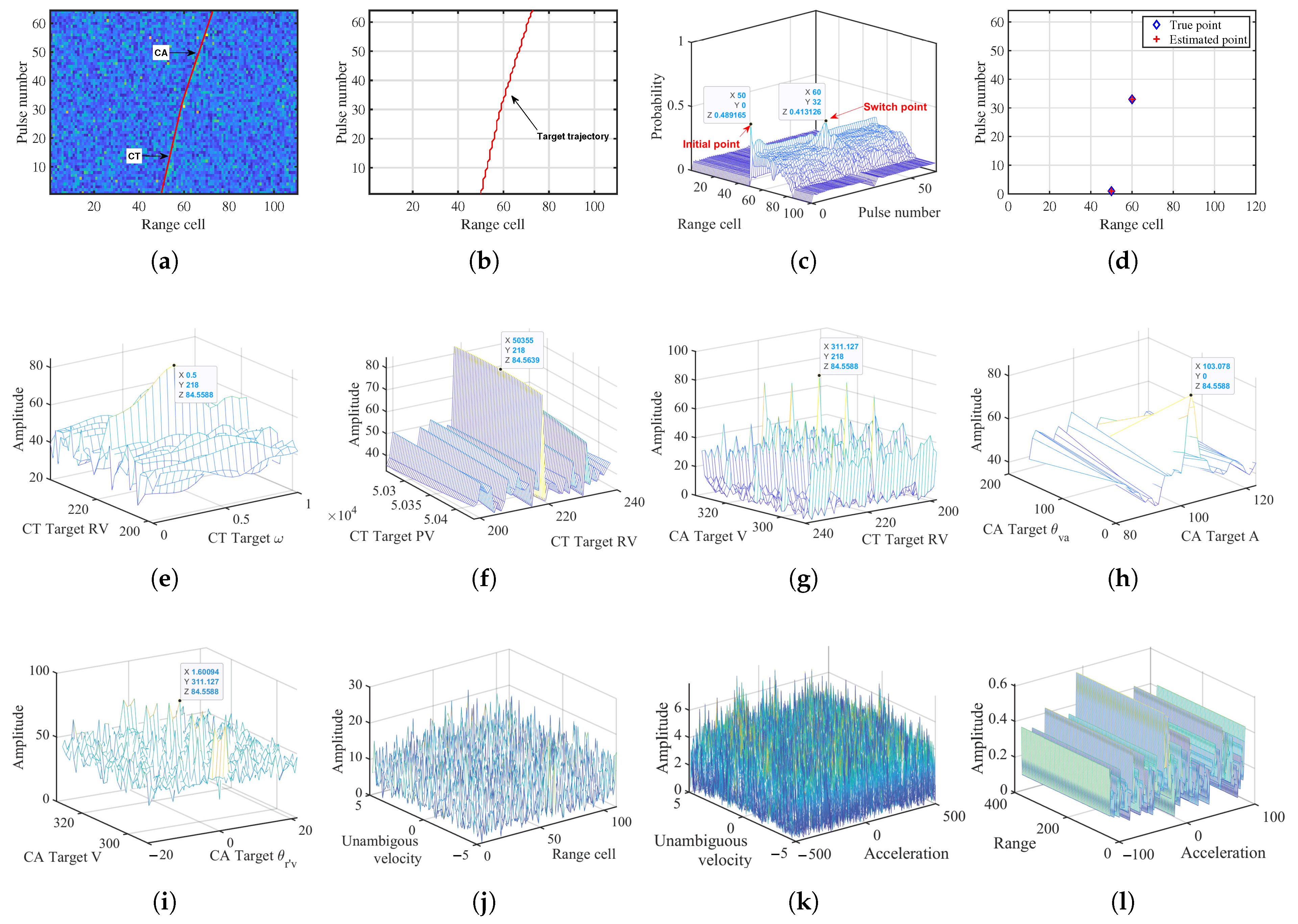
Case 3: In the CTCA motion scenario, the CTCA target’s motion parameters are: the initial Cartesian position is $(p_{x,0}^{\mathrm{CT}},p_{y,0}^{\mathrm{CT}})$ = $(112.5\mathrm{m},150\mathrm{m})$, the velocity of the target is $(v_x^{\mathrm{CT}},v_y^{\mathrm{CT}})$ = $(165\mathrm{m}/\mathrm{s},155\mathrm{m}/\mathrm{s})$, the turn rate is ${\omega }_{\mathrm{CT},0}=0.5\mathrm{rad}/\mathrm{s}$. When the motion mode switches from CT to CA, the velocity of the target is $(v_x^{\mathrm{CA}},v_y^{\mathrm{CA}})=(210\mathrm{m}/\mathrm{s},220\mathrm{m}/\mathrm{s})$, the acceleration of the target is $(a_x^{\mathrm{CA}},a_y^{\mathrm{CA}})=(75{\mathrm{m}/\mathrm{s}}^2,85{\mathrm{m}/\mathrm{s}}^2)$. The mode-switching occurs at the 32nd pulse. The SNR after PC is 2 dB. The true value of the target parameter is calculated to be $({\dot{r}}_{\mathrm{CT},0},{\sigma }_{\mathrm{CT},0},{\omega }_{\mathrm{CT},0},v_{\mathrm{CA},t_{\gamma }},a_{\mathrm{CA},t_{\gamma }},{\theta }_{va,t_{\gamma }},{\theta }_{\dot{r}v,t_{\gamma }})=(218\mathrm{m}/\mathrm{s},50350{\mathrm{m}}^2/{\mathrm{s}}^2,0.5\mathrm{rad}/\mathrm{s},311.13\mathrm{m}/\mathrm{s},103.08{\mathrm{m}/\mathrm{s}}^2,0°,1.60°)$.

Figure 5a displays the pulse-compressed signal with a SNR of 2 dB. Figure 5b shows the target trajectory marked by a solid line. Figure 5c presents the probability heatmap generated by the KDNet output. Figure 5d shows the comparative result between the ground truth keypoints and the estimated keypoints. Figure 5e displays the estimated radial velocity ${\widehat{\dot{r}}}_{\mathrm{CT},0}$ and the estimated turn rate ${\widehat{\omega }}_{\mathrm{CT},0}$ during the CT phase. Figure 5f presents the estimated pseudo velocity ${\widehat{\sigma }}_{\mathrm{CT},0}$ and estimated radial velocity ${\widehat{\dot{r}}}_{\mathrm{CT},0}$ during the CT phase. Figure 5g shows the estimated velocity ${\widehat{v}}_{\mathrm{CA},t_{\gamma }}$ during the CA phase and estimated radial velocity ${\widehat{\dot{r}}}_{\mathrm{CT},0}$ during the CT phase. Figure 5h presents the estimated angle ${\widehat{\theta }}_{va,t_{\gamma }}$ and estimated acceleration ${\widehat{a}}_{\mathrm{CA},t_{\gamma }}$ during the CA phase. Figure 5i displays the estimated angle ${\widehat{\theta }}_{\dot{r}v,t_{\gamma }}$ and the estimated velocity ${\widehat{v}}_{\mathrm{CA},t_{\gamma }}$ during the CA phase. Figure 5j displays the integration results of MTD. Figure 5k shows the integration results of FCN-dechirp. Figure 5l presents the integration results of third-order GRFT.

As illustrated in Figure 5e–i, the estimated target parameters are obtained as $({\widehat{\dot{r}}}_{\mathrm{CT},0},{\widehat{\sigma }}_{\mathrm{CT},0},{\widehat{\omega }}_{\mathrm{CT},0},{\widehat{v}}_{\mathrm{CA},t_{\gamma }},{\widehat{a}}_{\mathrm{CA},t_{\gamma }},{\widehat{\theta }}_{va,t_{\gamma }},{\widehat{\theta }}_{\dot{r}v,t_{\gamma }})$ = $(218\mathrm{m}/\mathrm{s},50355{\mathrm{m}}^2/{\mathrm{s}}^2,0.5\mathrm{rad}/\mathrm{s},311.13\mathrm{m}/\mathrm{s},103.08{\mathrm{m}/\mathrm{s}}^2,0°,1.60°)$. The results verify that the proposed algorithm reliably localizes both the initial and switch points, producing parameter estimates that closely match the ground-truth references.

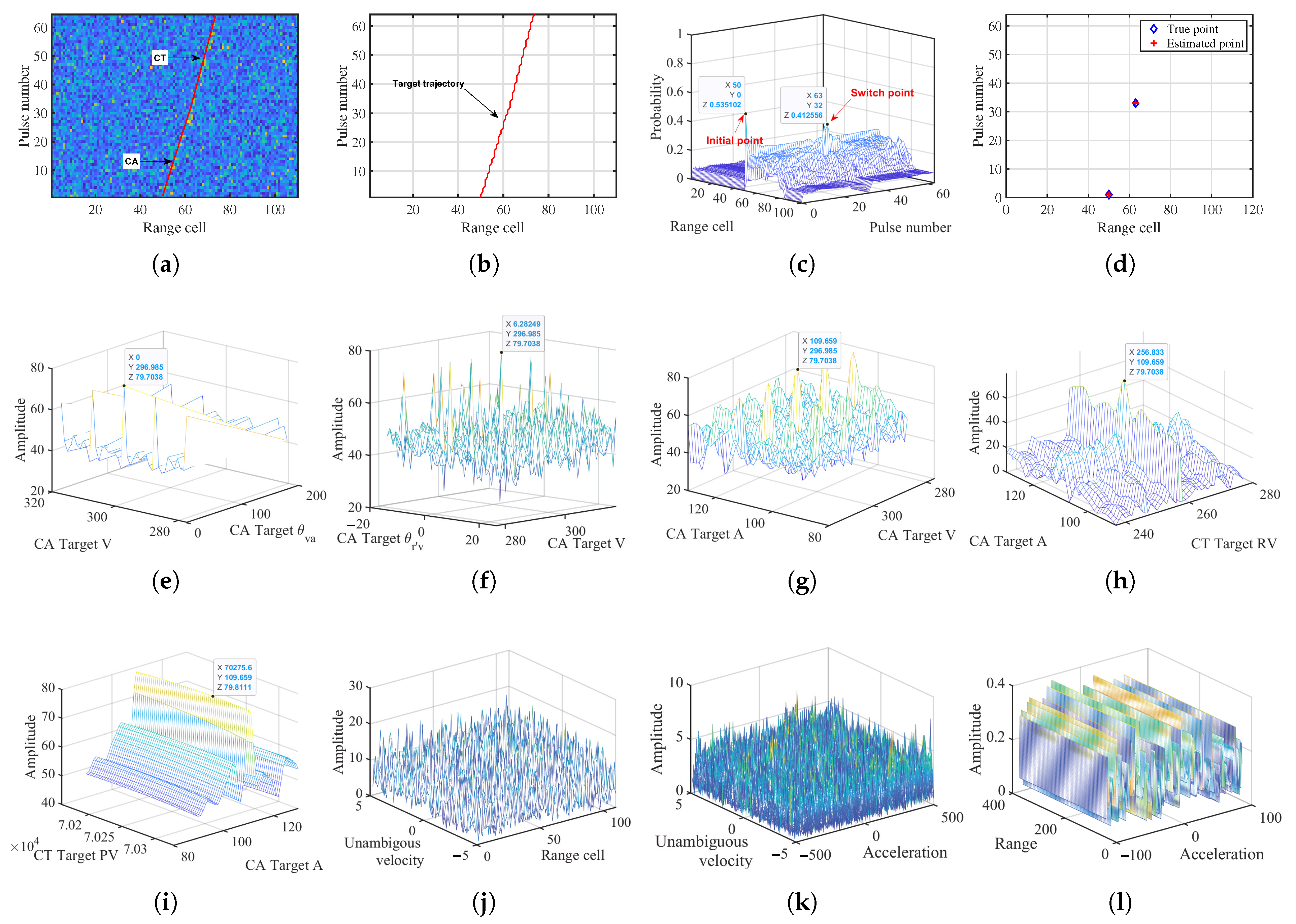
Case 4: In the CACT motion scenario, the CACT target’s motion parameters are as follows: the initial Cartesian position is $(p_{x,0}^{\mathrm{CA}},p_{y,0}^{\mathrm{CA}})=(112.5\mathrm{m},150\mathrm{m})$, the velocity of the target is $(v_x^{\mathrm{CA}},v_y^{\mathrm{CA}})=(210\mathrm{m}/\mathrm{s},210\mathrm{m}/\mathrm{s})$, the acceleration of the target is $(a_x^{\mathrm{CA}},a_y^{\mathrm{CA}})=(75{\mathrm{m}/\mathrm{s}}^2,80{\mathrm{m}/\mathrm{s}}^2)$. When the motion mode switches from CA to CT, the velocity of the target is $v_x^{\mathrm{CT}},v_y^{\mathrm{CT}}=(180\mathrm{m}/\mathrm{s},185\mathrm{m}/\mathrm{s})$, the turn rate is ${\omega }_{\mathrm{CT},t_{\gamma }}=0.6\mathrm{rad}/\mathrm{s}$. The mode-switching occurs at the 32nd pulse. The SNR after PC is 2 dB. The true value of the target parameter is calculated to be $(v_{\mathrm{CA},0},a_{\mathrm{CA},0},{\theta }_{va,0},{\theta }_{\dot{r}v,0},{\dot{r}}_{\mathrm{CT},t_{\gamma }},{\sigma }_{\mathrm{CT},t_{\gamma }},{\omega }_{\mathrm{CT},t_{\gamma }})$ = $(296.98\mathrm{m}/\mathrm{s},109.66{\mathrm{m}/\mathrm{s}}^2,0°,6.28°,256.83\mathrm{m}/\mathrm{s},70244{\mathrm{m}}^2/{\mathrm{s}}^2,0.6\mathrm{rad}/\mathrm{s})$.

Figure 6a displays the pulse-compressed signal with a SNR of 2 dB. Figure 6b shows the target trajectory marked by a solid line. Figure 6c presents the probability heatmap generated by the KDNet output. Figure 6d shows the comparative result between the ground truth keypoints and the estimated keypoints. Figure 6e displays the estimated velocity ${\widehat{v}}_{\mathrm{CA},0}$ and estimated angle ${\widehat{\theta }}_{va,0}$ during the CA phase. Figure 6f presents the estimated angle ${\widehat{\theta }}_{\dot{r}v,0}$ and the estimated velocity ${\widehat{v}}_{\mathrm{CA},0}$ during the CA phase. Figure 6g shows the estimated acceleration ${\widehat{a}}_{\mathrm{CA},0}$ and estimated velocity ${\widehat{v}}_{\mathrm{CA},0}$ during the CA phase. Figure 6h displays the estimated acceleration ${\widehat{a}}_{\mathrm{CA},0}$ during the CA phase and estimated radial velocity ${\widehat{\dot{r}}}_{\mathrm{CT},t_{\gamma }}$ during the CT phase. Figure 6i displays the estimated pesudo velocity ${\widehat{\sigma }}_{\mathrm{CT},t_{\gamma }}$ during the CT phase and the estimated acceleration ${\widehat{a}}_{\mathrm{CA},0}$ during the CA phase. Figure 6j show the integration results of MTD. Figure 6k displays the integration results of FCN-dechirp. Figure 6l presents the integration results of third-order GRFT.

As illustrated in Figure 6e–i, the estimated target parameters are obtained as $({\widehat{v}}_{\mathrm{CA},0},{\widehat{a}}_{\mathrm{CA},0},{\widehat{\theta }}_{va,0},{\widehat{\theta }}_{\dot{r}v,0},{\widehat{\dot{r}}}_{\mathrm{CT},t_{\gamma }},{\widehat{\sigma }}_{\mathrm{CT},t_{\gamma }},{\widehat{\omega }}_{\mathrm{CT},t_{\gamma }})$ = $(296.98\mathrm{m}/\mathrm{s},109.66{\mathrm{m}/\mathrm{s}}^2,0°,6.28°,$$256.83\mathrm{m}/\mathrm{s},70275.6{\mathrm{m}}^2/{\mathrm{s}}^2,0.6\mathrm{rad}/\mathrm{s})$. The results indicate that the proposed algorithm achieves accurate estimation of both the initial and switch points, yielding parameter estimates that remain closely aligned with the ground-truth values.

From the above four simulation scenarios, it can be observed that, compared with the MTD, FCN-dechirp, and GRFT, the proposed method achieves superior detection performance and parameter estimation accuracy. Specifically, the MTD algorithm requires that the target is confined to a single range-Doppler cell, and its coherent integration performance degrades significantly when mode-switching occurs. The FCN-dechirp algorithm is limited by its network architecture and feature extraction ability, making it difficult to accurately estimate the target trajectory and thus leading to notable parameter-estimation errors. The GRFT algorithm performs energy integration using a single high-order range equation and fails to capture the piecewise motion characteristics under mode-switching conditions, which also prevents it from achieving accurate parameter estimates. In contrast, the proposed method can accurately localize the keypoints along the target trajectory and perform piecewise coherent integration, yielding parameter estimates that are close to the ground truth. Therefore, the proposed method outperforms the competing approaches in both detection capability and parameter-estimation performance.

4.3. Integration for Multiple Target

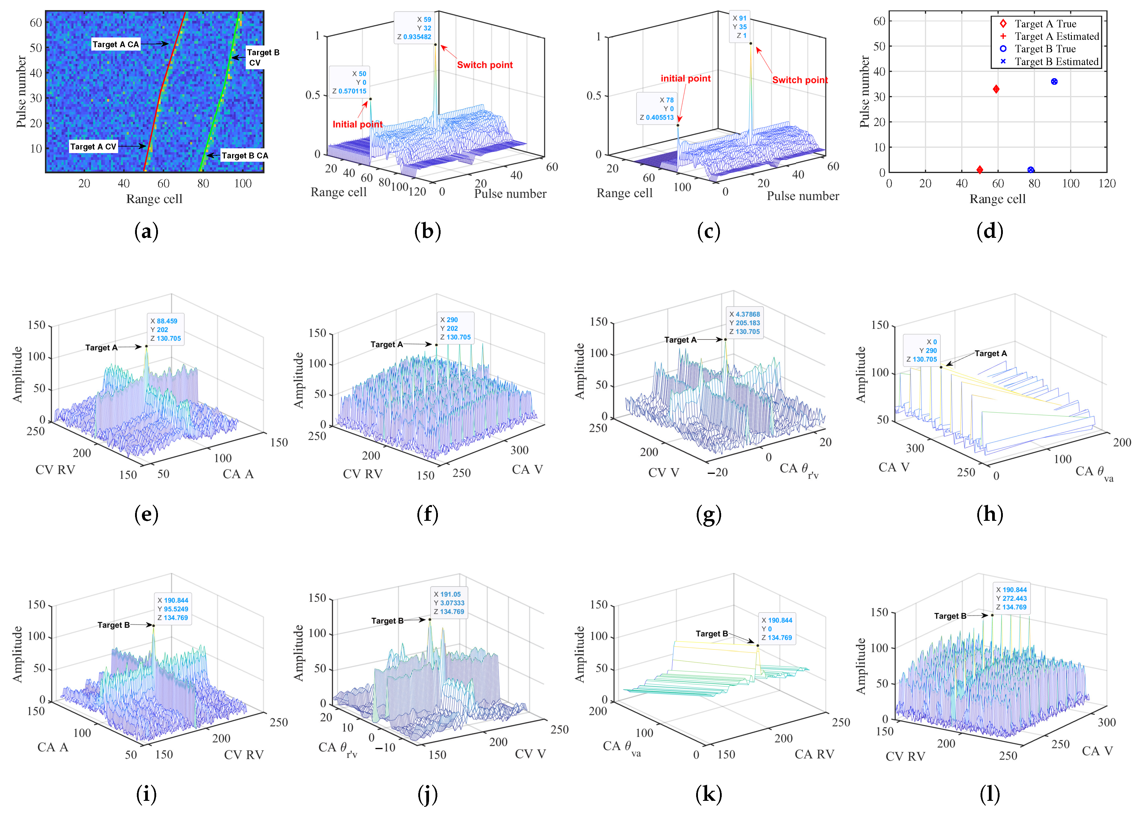
Due to space limitations, we discuss only the cases involving CVCA and CACV here. Two targets, denoted by Target A and Target B, whose motion parameters are given in

Table 7. The motion parameters of Target A and Target B.

Parameters	Target A CV	Target A CA	Target B CA	Target B CV
Position	(112.5 m, 150 m)	-	(187.5 m, 225 m)	-
Velocity	(150 m/s, 140 m/s)	(185 m/s, 152 m/s)	(185 m/s, 200 m/s)	(130 m/s, 140 m/s)
Acceleration	-	(60${\mathrm{m}/\mathrm{s}}^2$, 65${\mathrm{m}/\mathrm{s}}^2$)	(65${\mathrm{m}/\mathrm{s}}^2$, 70${\mathrm{m}/\mathrm{s}}^2$)	-

. The radar parameters show in Table 4. Target A demonstrates a CVCA motion with mode-switching occurring at the 58th range cell and 32nd pulse, while Target B exhibits a CACV motion, showing mode-switching behavior at the 91st range cell and 35th pulse. The SNR after PC is 7 dB. The true value of the Target A parameter is $\left({\dot{r}}_{\mathrm{CV},0},v_{\mathrm{CV},0},v_{\mathrm{CA},t_{\gamma }},a_{\mathrm{CA},t_{\gamma }},{\theta }_{va,t_{\gamma }},{\theta }_{\dot{r}v,t_{\gamma }}\right)$ = $(202\mathrm{m}/\mathrm{s},205.18\mathrm{m}/\mathrm{s},290\mathrm{m}/\mathrm{s},88.46{\mathrm{m}/\mathrm{s}}^2,0°,$$4.38°)$. The true value of the Target B parameter is $\left(v_{\mathrm{CA},0},a_{\mathrm{CA},0},{\theta }_{va,0},{\theta }_{\dot{r}v,0},{\dot{r}}_{\mathrm{CV},t_{\gamma }},v_{\mathrm{CV},t_{\gamma }}\right)$ = $(272.44\mathrm{m}/\mathrm{s},95.52{\mathrm{m}/\mathrm{s}}^2,0°,3.07°,190.84\mathrm{m}/\mathrm{s},191.05\mathrm{m}/\mathrm{s})$.

Figure 7a displays the pulse-compressed signal with a SNR of 7 dB. Figure 7b shows the probability heatmap generated by the KDNet output for the CVCA target. Figure 7c presents the probability heatmap generated by the KDNet output for the CACV target. Figure 7d shows the comparative result between the ground truth keypoints and the estimated keypoints. Figure 7e displays the estimated radial velocity ${\widehat{\dot{r}}}_{\mathrm{CV},0}$ during the CV phase and the estimated acceleration ${\widehat{a}}_{\mathrm{CA},t_{\gamma }}$ during the CA phase of Target A. Figure 7f shows the estimated radial velocity ${\widehat{\dot{r}}}_{\mathrm{CV},0}$ during the CV phase and the estimated velocity ${\widehat{v}}_{\mathrm{CA},t_{\gamma }}$ during the CA phase of Target A. Figure 7g presents the estimated velocity ${\widehat{v}}_{\mathrm{CA},t_{\gamma }}$ and the estimated angle ${\widehat{\theta }}_{\dot{r}v,t_{\gamma }}$ during the CA phase of Target A. Figure 7h displays the estimated velocity ${\widehat{v}}_{\mathrm{CA},t_{\gamma }}$ and the estimated angle ${\widehat{\theta }}_{va,t_{\gamma }}$ during the CA phase of Target A. Figure 7i shows the estimated acceleration ${\widehat{a}}_{\mathrm{CA},0}$ during the CA phase and the estimated radial velocity ${\widehat{\dot{r}}}_{\mathrm{CV},t_{\gamma }}$ during the CV phase of Target B. Figure 7j presents the estimated angle ${\widehat{\theta }}_{\dot{r}v,0}$ during the CA phase and the estimated velocity ${\widehat{v}}_{\mathrm{CV},t_{\gamma }}$ during the CV phase of Target B. Figure 7k displays the estimated angle ${\widehat{\theta }}_{va,0}$ and the estimated radial velocity ${\widehat{\dot{r}}}_{\mathrm{CA},0}$ during the CA phase of Target B. Figure 7l shows the estimated radial velocity ${\widehat{\dot{r}}}_{\mathrm{CV},t_{\gamma }}$ during the CV phase and the estimated velocity ${\widehat{v}}_{\mathrm{CA},0}$ during the CA phase of Target B.

As illustrated in Figure 7e–h, the estimated parameters of Target A are obtained as $({\widehat{\dot{r}}}_{\mathrm{CV},0},{\widehat{v}}_{\mathrm{CV},0},{\widehat{v}}_{\mathrm{CA},t_{\gamma }},{\widehat{a}}_{\mathrm{CA},t_{\gamma }},{\widehat{\theta }}_{va,t_{\gamma }},{\widehat{\theta }}_{\dot{r}v,t_{\gamma }})$ = $(202\mathrm{m}/\mathrm{s},205.18\mathrm{m}/\mathrm{s},290\mathrm{m}/\mathrm{s},88.46{\mathrm{m}/\mathrm{s}}^2,0°,$$4.38°)$, and the estimated parameters of Target B are obtained as $({\widehat{v}}_{\mathrm{CA},0},{\widehat{a}}_{\mathrm{CA},0},{\widehat{\theta }}_{va,0},{\widehat{\theta }}_{\dot{r}v,0},$${\widehat{\dot{r}}}_{\mathrm{CV},t_{\gamma }},{\widehat{v}}_{\mathrm{CV},t_{\gamma }})$ = $(272.44\mathrm{m}/\mathrm{s},95.52{\mathrm{m}/\mathrm{s}}^2,0°,3.07°,190.84\mathrm{m}/\mathrm{s},191.05\mathrm{m}/\mathrm{s})$. The results demonstrate that the proposed algorithm can accurately estimate both the initial point and the switch point for Target A and Target B, with parameter estimates closely approximating their respective ground-truth values. This improvement primarily stems from the fact that the proposed method can effectively extract keypoint features of target trajectories, thereby enabling accurate detection and estimation of the keypoint locations for different targets and yielding superior energy focusing and parameter-estimation performance in piecewise coherent integration. Notably, in the context of sliding window detection, for any given target, energy focusing occurs solely when the estimated keypoints match the target’s true trajectory. Furthermore, introducing ID tracking is also an effective approach to avoid ambiguity in multi-target detection.

4.4. Detection Performance

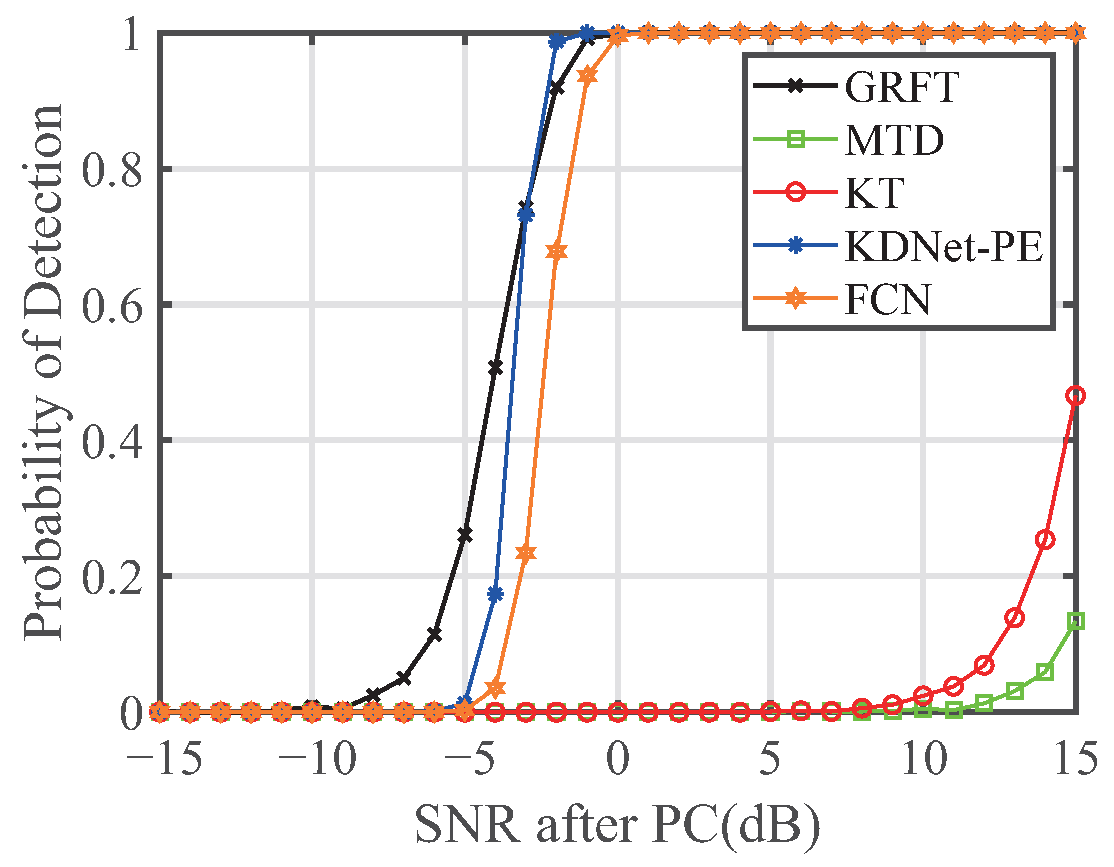
To evaluate the detection performance of the proposed algorithm, Monte Carlo simulations are conducted to compare the proposed method with the GRFT, FCN, KT, and MTD. The test parameters are set as follows: the false alarm probability is $P_{fa}={10}^{-6}$, and the post-pulse-compression SNR varies from −15 dB to 15 dB. For each SNR level, 1000 Monte Carlo trials are performed. Figure 8 illustrates the relationship between the detection probability and the SNR. As shown in the figure, the detection performance in descending order is as follows: GRFT, KDNet, FCN, KT, and MTD. When the detection probability reaches 80%, the SNRs required by KDNet and the FCN are approximately 0.2 dB and 2 dB higher than that of the GRFT, respectively. In comparison, the KT and MTD methods suffer from the limitations imposed by RM and DFM, which lead to degraded detection performance. Moreover, the FCN fails to accurately estimate the target trajectory, thereby preventing reliable estimation of the target’s motion parameters. The performance of KDNet approaches that of the GRFT algorithm, which is considered near-optimal. Experimental results further indicate that the proposed approach sustains reliable detection capability in low-SNR environments, attaining performance comparable to that of GRFT.

4.5. Keypoint Detection Performance

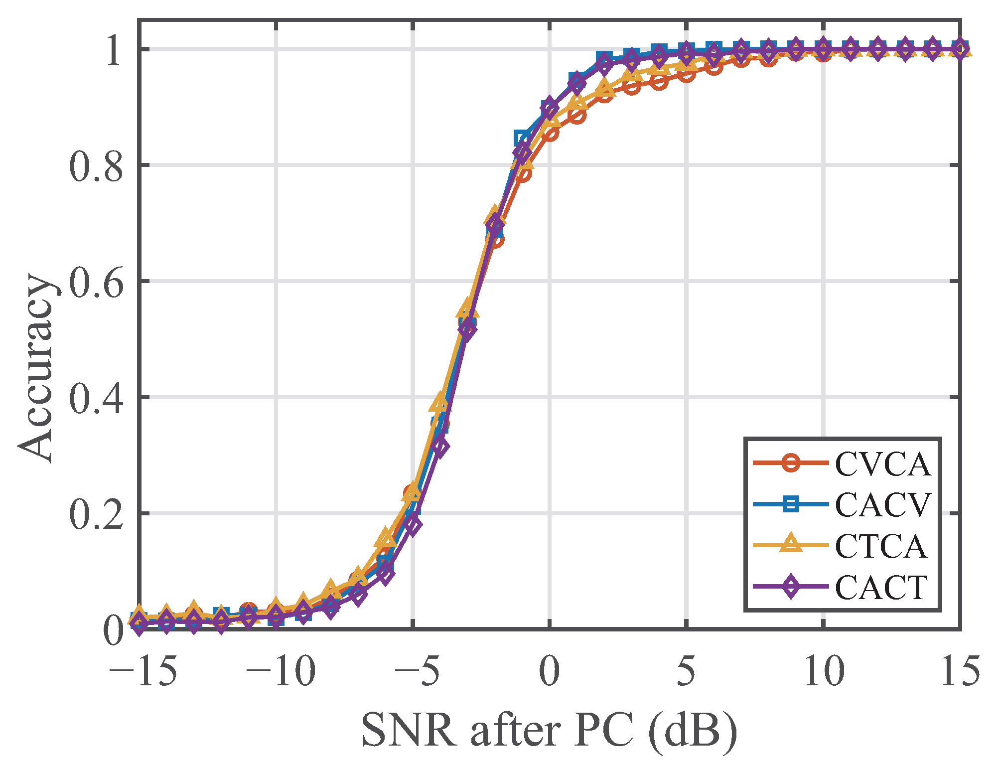
In this section, we evaluate the keypoint detection performance across different SNRs. The target parameters employed in this evaluation are consistent with those in Case 1 to Case 4. We conducted 1000 Monte Carlo trials for each scenario at every SNR level, spanning a range from $-15$ dB to 15 dB. As illustrated in Figure 9, the keypoint detection accuracy ${\mathcal{A}}_{\mathrm{avg}}$ exhibits a rapid upward trend within the SNR range of $-5$ dB to 5 dB. Specifically, the average accuracy reaches approximately 85% at 0 dB and converges to nearly 100% for SNRs above 5 dB. These results demonstrate superior detection performance, effectively verifying the reliability of the proposed algorithm in precise keypoint localization.

4.6. Computational Cost Analysis

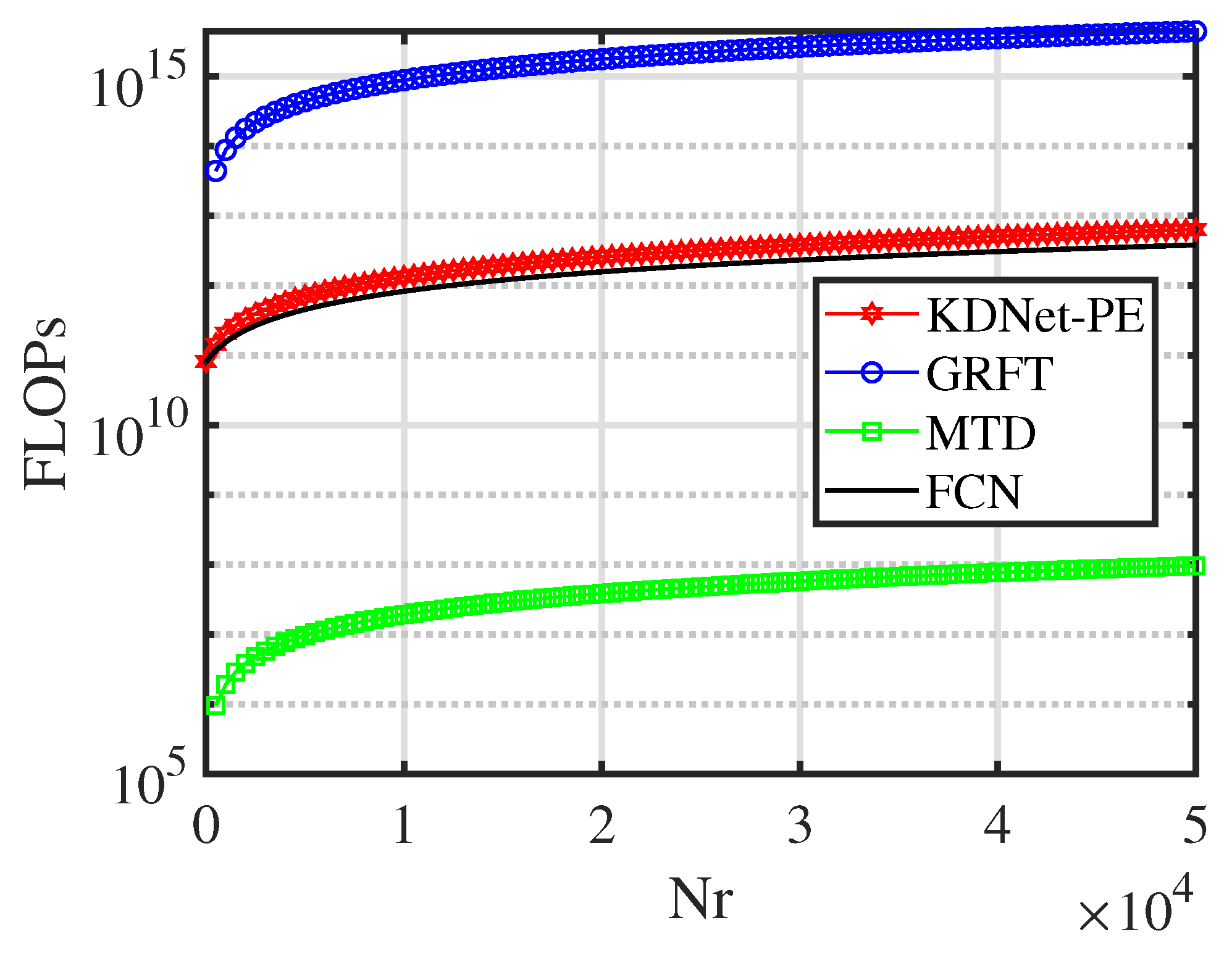
In this section, the computational complexities of various algorithms are analyzed and compared. The algorithms involved in the comparison include KDNet-PE, FCN, GRFT, and MTD. As shown in Figure 10, the computational cost, ranked from lowest to highest, is MTD, FCN, KDNet-PE, and GRFT. The computational complexity of the GRFT is 38.63 times higher than that of KDNet-PE. The computational complexity of KDNet-PE is 1.67 times higher than that of FCN. The practical running time shows in

Table 8. Practical running time.

Algorithm	Time (s)
GRFT	9737.3
KDNet-PE	276.2
MTD	1.6
FCN	170.3

Hardware configuration: Intel Core Ultra 9 CPU @ 5.10GHz and NVIDIA GeForce RTX 4060 GPU; Software environment: MATLAB R2024a, Python 3.9, and PyTorch 1.13.1.

. The measured execution time aligns well with the algorithm’s theoretical complexity, though minor deviations may arise from hardware performance and other implementation-level factors.

5. Conclusions

This paper proposes a model–data dual-driven method for mode-switching radar target detection. From the model-driven perspective, the range evolution laws under various mode-switching conditions are derived in the Cartesian coordinate system, based on which a trajectory database is constructed to provide diverse training samples. From the data-driven perspective, a hierarchical residual network is designed to extract multi-scale features from radar echoes embedded with mode-switching targets. Additionally, a joint loss function, combining PAW-BCE loss and Wing loss, is introduced to supervise the precise localization of the trajectory’s initial and switching points. To enhance model interpretability, network output visualization is incorporated to provide an intuitive representation of keypoint information. Leveraging the detected switching points, the candidate CPI is determined, followed by a parameter search to achieve target focusing and parameter estimation. Simulation results across different mode-switching scenarios demonstrate that the proposed approach effectively mitigates the effects of RM and DFM. The accurate range-evolution modeling and precise keypoint estimation jointly ensure efficient energy integration and reliable parameter estimation, compared with existing coherent integration methods. Validating the proposed method with real radar data, exploring its robustness in complex electromagnetic environments, and optimizing the search efficiency via a hierarchical subspace search strategy remain important directions for our future work.

References

1. Chen, Z.; Peng, X.; Yang, J.; Zhong, Z.; Song, Q.; Zhang, Y. A Hybrid Integration Method Based on SMC-PHD-TBD for Multiple High-Speed and Highly Maneuverable Targets in Ubiquitous Radar. Remote Sens. 2024, 16, 2618. [Google Scholar] [CrossRef] [Scilit]
2. Liu, G.; Tian, Y.; Wen, B.; Liu, C. Combined Coherent and Non-Coherent Long-Time Integration Method for High-Speed Target Detection Using High-Frequency Radar. Remote Sens. 2024, 16, 2139. [Google Scholar] [CrossRef] [Scilit]
3. Gao, L.; Li, X.; Wang, M.; Sun, Z.; Cui, G.; Yeo, T. Multichannel Multiframe Integration Detection Method for Weak Target With Coherent MIMO Radar. IEEE Trans. Aerosp. Electron. Syst. 2025, 61, 6518–6536. [Google Scholar] [CrossRef] [Scilit]
4. Wang, J.; Wu, Y.; Deng, X.; Zhang, L.; Wang, J.; Zhou, L. Highly Maneuvering Target Detection Based on Neural Network and Generalized Radon-Fourier Transform. IEEE Geosci. Remote. Sens. Lett. 2023, 20, 1–5. [Google Scholar] [CrossRef] [Scilit]
5. Carlson, B.; Evans, E.; Wilson, S. Search radar detection and track with the Hough transform. I. system concept. IEEE Trans. Aerosp. Electron. Syst. 1994, 30, 102–108. [Google Scholar] [CrossRef] [Scilit]
6. Carlson, B.; Evans, E.; Wilson, S. Search radar detection and track with the Hough transform. II. detection statistics. IEEE Trans. Aerosp. Electron. Syst. 1994, 30, 109–115. [Google Scholar] [CrossRef] [Scilit]
7. Carlson, B.; Evans, E.; Wilson, S. Search radar detection and track with the Hough transform. III. Detection performance with binary integration. IEEE Trans. Aerosp. Electron. Syst. 1994, 30, 116–125. [Google Scholar] [CrossRef] [Scilit]
8. Yu, J.; Xu, J.; Peng, Y.; Xia, X. Radon-Fourier Transform for Radar Target Detection (III): Optimality and Fast Implementations. IEEE Trans. Aerosp. Electron. Syst. 2012, 48, 991–1004. [Google Scholar] [CrossRef] [Scilit]
9. Chen, X.; Guan, J.; Chen, W.; Zhang, L.; Yu, X. Sparse long-time coherent integration-based detection method for radar low-observable manoeuvring target. IET Radar Sonar Navig. 2020, 14, 538–546. [Google Scholar] [CrossRef] [Scilit]
10. Perry, R.; DiPietro, R.; Fante, R. SAR imaging of moving targets. IEEE Trans. Aerosp. Electron. Syst. 1999, 35, 188–200. [Google Scholar] [CrossRef] [Scilit]
11. Perry, R.; DiPietro, R.; Fante, R. Coherent integration with range migration using keystone formatting. In Proceedings of the IEEE Radar Conference, Boston, MA, USA, 17–20 April 2007; pp. 863–868. [Google Scholar]
12. Kong, L.; Li, X.; Cui, G.; Yi, W.; Yang, Y. Coherent Integration Algorithm for a Maneuvering Target With High-Order Range Migration. IEEE Trans. Signal Process. 2015, 63, 4474–4486. [Google Scholar] [CrossRef] [Scilit]
13. Li, X.; Cui, G.; Yi, W.; Kong, L. A Fast Maneuvering Target Motion Parameters Estimation Algorithm Based on ACCF. IEEE Signal Process. Lett. 2015, 22, 270–274. [Google Scholar] [CrossRef] [Scilit]
14. Li, X.; Cui, G.; Yi, W.; Kong, L. Sequence-Reversing Transform-Based Coherent Integration for High-Speed Target Detection. IEEE Trans. Aerosp. Electron. Syst. 2017, 53, 1573–1580. [Google Scholar] [CrossRef] [Scilit]
15. Li, X.; Cui, G.; Yi, W.; Kong, L. Radar maneuvering target detection and motion parameter estimation based on TRT-SGRFT. Signal Process. 2017, 133, 107–116. [Google Scholar] [CrossRef] [Scilit]
16. Zheng, J.; Su, T.; Zhu, W.; He, X.; Liu, Q. Radar High-Speed Target Detection Based on the Scaled Inverse Fourier Transform. IEEE J. Sel. Top. Appl. Earth Observ. Remote Sens. 2015, 8, 1108–1119. [Google Scholar] [CrossRef] [Scilit]
17. Zheng, J.; Su, T.; Liu, H.; Liao, G.; Liu, Z.; Liu, Q. Radar High-Speed Target Detection Based on the Frequency-Domain Deramp-Keystone Transform. IEEE J. Sel. Top. Appl. Earth Observ. Remote Sens. 2016, 9, 285–294. [Google Scholar] [CrossRef] [Scilit]
18. Xu, J.; Xia, X.; Peng, S.; Yu, J.; Peng, Y.; Qian, L. Radar Maneuvering Target Motion Estimation Based on Generalized Radon-Fourier Transform. IEEE Trans. Signal Process. 2012, 60, 6190–6201. [Google Scholar] [CrossRef] [Scilit]
19. Li, X.; Sun, Z.; Yeo, T.; Zhang, T.; Yi, W.; Cui, G.; Kong, L. STGRFT for Detection of Maneuvering Weak Target With Multiple Motion Models. IEEE Trans. Signal Process. 2019, 67, 1902–1917. [Google Scholar] [CrossRef] [Scilit]
20. Wang, J.; Li, S. Maritime Radar Target Detection Model Self-Evolution Based on Semisupervised Learning. IEEE Trans. Geosci. Remote Sens. 2024, 62, 1–11. [Google Scholar] [CrossRef] [Scilit]
21. Su, N.; Chen, X.; Guan, J.; Huang, Y.; Wang, X.; Xue, Y. Radar Maritime Target Detection via Spatial-Temporal Feature Attention Graph Convolutional Network. IEEE Trans. Geosci. Remote Sens. 2024, 62, 1–15. [Google Scholar] [CrossRef] [Scilit]
22. Yan, B.; Li, Y.; Kou, Q.; Chen, R.; Ren, Z.; Cheng, W.; Dong, L.; Luan, L. A Deep Learning-Based Method for Detection of Multiple Maneuvering Targets and Parameter Estimation. Remote Sens. 2025, 17, 2574. [Google Scholar] [CrossRef] [Scilit]
23. Jiang, W.; Liu, H.; Jiu, B.; Zhao, Y.; Li, K.; Zhang, Y. Full-Dimensional Partial-Search Generalized Radon-Fourier Transform for High-Speed Maneuvering Target Detection. IEEE Trans. Aerosp. Electron. Syst. 2024, 60, 5445–5457. [Google Scholar] [CrossRef] [Scilit]
24. Wang, C.; Zheng, J.; Jiu, B.; Liu, H. Model-and-Data-Driven Method for Radar Highly Maneuvering Target Detection. IEEE Trans. Aerosp. Electron. Syst. 2021, 57, 2201–2217. [Google Scholar] [CrossRef] [Scilit]
25. Wang, B.; Zhou, G. Multiscale Feature Learning Based on Deep Pyramid Residual Shrinking Network for Radar Target Detection. IEEE Trans. Aerosp. Electron. Syst. 2025, 61, 3544–3563. [Google Scholar] [CrossRef] [Scilit]
26. Chen, W.; Sang, H.; Wang, J.; Zhao, Z. DSTIGCN: Deformable Spatial-Temporal Interaction Graph Convolution Network for Pedestrian Trajectory Prediction. IEEE Trans. Intell. Transp. Syst. 2025, 26, 6923-–6935. [Google Scholar] [CrossRef] [Scilit]
27. Li, W.; Zhang, Y.; Li, L.; Lv, Y.; Wang, M. A Pedestrian Trajectory Prediction Model for Right-Turn Unsignalized Intersections Based on Game Theory. IEEE Trans. Intell. Transp. Syst. 2024, 25, 9643-–9658. [Google Scholar] [CrossRef] [Scilit]
28. Wong, C.; Xia, B.; Zou, Z.; Wang, Y.; You, X. SocialCircle: Learning the Angle-based Social Interaction Representation for Pedestrian Trajectory Prediction. In Proceedings of the IEEE/CVF Conference on Computer Vision and Pattern Recognition (CVPR), Seattle, WA, USA, 16–22 June 2024; pp. 19005–19015. [Google Scholar]
29. Zheng, S.; Zhou, X.; Zhang, L.; Qi, P.; Qiu, K.; Zhu, J.; Yang, X. Toward Next-Generation Signal Intelligence: A Hybrid Knowledge and Data-Driven Deep Learning Framework for Radio Signal Classification. IEEE Trans. Cogn. Commun. 2023, 9, 564–579. [Google Scholar] [CrossRef] [Scilit]
30. Li, X.; Jilkov, V. Survey of maneuvering target tracking. Part I: Dynamic models. IEEE Trans. Aerosp. Electron. Syst. 2003, 39, 1333–1364. [Google Scholar]
31. Huang, D.; Xue, A.; Guo, Y. Penalty Dynamic Programming Algorithm for Dim Targets Detection in Sensor Systems. Sensors 2012, 12, 5028–5046. [Google Scholar] [CrossRef] [Scilit] [PubMed]
32. Wang, L.; Zhou, G. A unified method based on pseudo-spectrum for track-before-detect of targets with motion model uncertainty. Digit. Signal Process. 2021, 114, 103078. [Google Scholar] [CrossRef] [Scilit]
33. Mark, A.R. Fundamentals of Radar Signal Processing; McGraw-Hill: New York, NY, USA, 2005. [Google Scholar]
Figure 1. The labels of the target trajectory.
Remotesensing 18 00144 g001
Figure 2. The overall structure of the proposed method.
Remotesensing 18 00144 g002
Figure 3. Integration for a single CVCA target. (a) The pulse-compressed signal with a SNR of 2 dB. (b) The trajectory of CVCA target. (c) Probability heatmap generated by the KDNet output. (d) The comparative result between the ground truth keypoints and the estimated keypoints. (e) The estimated radial velocity r ˙ ^ CV , 0 and the estimated velocity v ^ CV , 0 during the CV phase. (f) The estimated radial velocity r ˙ ^ CV , 0 during the CV phase and the estimated velocity v ^ CA , t γ during the CA phase. (g) The estimated velocity v ^ CA , t γ and the estimated angle θ ^ v a during the CA phase. (h) The estimated velocity v ^ CV , 0 during the CV phase and the estimated angle θ ^ r ˙ v during the CA phase. (i) The estimated radial velocity r ˙ ^ CV , 0 during the CV phase and the estimated acceleration a ^ CA , t γ during the CA phase. (j) Result of MTD. (k) Result of FCN-dechirp. (l) Result of third-order GRFT.
Remotesensing 18 00144 g003
Figure 4. Integration for a single CACV target. (a) The pulse-compressed signal with a SNR of 2 dB. (b) The trajectory of CACV target. (c) Probability heatmap generated by the KDNet output. (d) The comparative result between the ground truth keypoints and the estimated keypoints. (e) The estimated velocity v ^ CA , 0 and the estimated θ ^ v a during the CA phase. (f) The estimated velocity v ^ CA , 0 and the estimated angle θ ^ r ˙ a during the CA phase. (g) The estimated acceleration a ^ CA , 0 during the CA phase and the estimated radial velocity r ˙ ^ CV , t γ during the CV phase. (h) The estimated velocity v ^ CV , t γ during the CV phase and the estimated velocity v ^ CA , 0 during the CA phase. (i) The estimated radial velocity r ˙ ^ CV , t γ during the CV phase and the estimated angle θ ^ v a during the CA phase. (j) Result of MTD. (k) Result of FCN-dechirp. (l) Result of third-order GRFT.
Remotesensing 18 00144 g004
Figure 5. Integration for a single CTCA target. (a) The pulse-compressed signal with a SNR of 2 dB. (b) The trajectory of CTCA target. (c) Probability heatmap generated by the KDNet output. (d) The comparative result between the ground truth keypoints and the estimated keypoints. (e) The estimated radial velocity r ˙ ^ CT , 0 and the estimated turn rate ω ^ CT , 0 during the CT phase. (f) The estimated radial velocity r ˙ ^ CT , 0 and the estimated pseudo velocity σ ^ CT , 0 during the CT phase. (g) The estimated velocity v ^ CA , t γ during the CA phase and estimated radial velocity r ˙ ^ CT , 0 during the CT phase. (h) The estimated angle θ ^ v a , t γ and estimated acceleration a ^ CA , t γ during the CA phase. (i) The estimated angle θ ^ r ˙ v , t γ and the estimated velocity v ^ CA , t γ during the CA phase. (j) Result of MTD. (k) Result of FCN-dechirp. (l) Result of third-order GRFT.
Remotesensing 18 00144 g005
Figure 6. Integration for a single CACT target. (a) The pulse-compressed signal with a SNR of 2 dB. (b) The trajectory of CACT target. (c) Probability heatmap generated by the KDNet output. (d) The comparative result between the ground truth keypoints and the estimated keypoints. (e) The estimated velocity v ^ CA , 0 and estimated angle θ ^ v a , 0 during the CA phase. (f) The estimated angle θ ^ r ˙ v , 0 and the estimated velocity v ^ CA , 0 during the CA phase. (g) The estimated acceleration a ^ CA , 0 and estimated velocity v ^ CA , 0 during the CA phase. (h) The estimated acceleration a ^ CA , 0 during the CA phase and estimated radial velocity r ˙ ^ CT , t γ during the CT phase. (i) The estimated pesudo velocity σ ^ CT , t γ during the CT phase and the estimated acceleration a ^ CA , 0 during the CA phase. (j) Result of MTD. (k) Result of FCN-dechirp. (l) Result of third-order GRFT.
Remotesensing 18 00144 g006
Figure 7. Integration for CVCA target and CACV target. (a) The pulse-compressed signal with a SNR of 7 dB. (b) Probability heatmap generated by the KDNet output for the CVCA target. (c) Probability heatmap generated by the KDNet output for the CACV target. (d) The comparative result between the ground truth keypoints and the estimated keypoints. (e) The estimated radial velocity r ˙ ^ CV , 0 during the CV phase and the estimated acceleration a ^ CA , t γ during the CA phase of Target A. (f) The estimated radial velocity r ˙ ^ CV , 0 during the CV phase and the estimated velocity v ^ CA , t γ during the CA phase of Target A. (g) The estimated velocity v ^ CA , t γ and the estimated angle θ ^ r ˙ v , t γ during the CA phase of Target A. (h) The estimated velocity v ^ CA , t γ and the estimated angle θ ^ v a , t γ during the CA phase of Target A. (i) The estimated acceleration a ^ CA , 0 during the CA phase and the estimated radial velocity r ˙ ^ CV , t γ during the CV phase of Target B. (j) The estimated angle θ ^ r ˙ v , 0 during the CA phase and the estimated velocity v ^ CV , t γ during the CV phase of Target B. (k) The estimated angle θ ^ v a , 0 and the estimated radial velocity r ˙ ^ CA , 0 during the CA phase of Target B. (l) The estimated radial velocity r ˙ ^ CV , t γ during the CV phase and the estimated velocity v ^ CA , 0 during the CA phase of Target B.
Remotesensing 18 00144 g007
Figure 8. Comparison of detection probabilities.
Remotesensing 18 00144 g008
Figure 9. The keypoint detection performance across different SNRs.
Remotesensing 18 00144 g009
Figure 10. The computational cost.
Remotesensing 18 00144 g010