IceBench: A Benchmark for Deep-Learning-Based Sea-Ice Type Classification

Abstract

Sea ice plays a critical role in the global climate system and maritime operations, making timely and accurate classification essential. However, traditional manual methods are time-consuming, costly, and have inherent biases. Automating sea-ice type classification addresses these challenges by enabling faster, more consistent, and scalable analysis. While both traditional and deep-learning approaches have been explored, deep-learning models offer a promising direction for improving efficiency and consistency in sea-ice classification. However, the absence of a standardized benchmark and comparative study prevents a clear consensus on the best-performing models. To bridge this gap, we introduce IceBench, a comprehensive benchmarking framework for sea-ice type classification. Our key contributions are three-fold: First, we establish the IceBench benchmarking framework, which leverages the existing AI4Arctic Sea Ice Challenge Dataset as a standardized dataset, incorporates a comprehensive set of evaluation metrics, and includes representative models from the entire spectrum of sea-ice type-classification methods categorized in two distinct groups, namely pixel-based classification methods and patch-based classification methods. IceBench is open-source and allows for convenient integration and evaluation of other sea-ice type-classification methods, hence facilitating comparative evaluation of new methods and improving reproducibility in the field. Second, we conduct an in-depth comparative study on representative models to assess their strengths and limitations, providing insights for both practitioners and researchers. Third, we leverage IceBench for systematic experiments addressing key research questions on model transferability across seasons (time) and locations (space), data downsampling, and preprocessing strategies. By identifying the best-performing models under different conditions, IceBench serves as a valuable reference for future research and a robust benchmarking framework for the field.

1. Introduction

Sea ice plays a pivotal role in the global climate system. It significantly impacts maritime operations, affecting shipping routes, resource exploration, and coastal communities in polar regions. As such, timely and accurate classification of sea-ice types is essential for a wide range of applications, from climate modeling to maritime safety [1,2,3]. Traditionally, sea-ice type classification has relied on manual ice charting methods [4,5]. Although ice charting has proven valuable, its reliance on human annotation makes the process time-consuming and costly. These limitations reduce its reliability, especially as the demand for large-scale, up-to-date, and accurate sea-ice classification grows in response to accelerating climate change.

To address these challenges, automating sea-ice classification has become increasingly important. Early methods relied on traditional machine learning, but deep learning captures intricate spatial and textural patterns directly from raw data. This shift has revolutionized sea-ice type classification, enhancing accuracy, scalability, and real-time mapping capabilities [6,7]. Deep-learning models require large amounts of data to train effectively and learn meaningful patterns. However, progress in deep-learning-based sea-ice type classification was initially hindered by the lack of publicly available datasets. Without sufficient labeled data, models struggled to generalize and reach their full potential. Recent efforts to develop and share large-scale datasets have addressed this limitation, providing valuable resources for training and evaluation [8]. As a result, deep-learning models can better learn intricate features directly from raw data, reducing the need for manual feature engineering and further enhancing classification accuracy.

While the availability of large-scale datasets has accelerated progress in deep-learning-based sea-ice classification, a major challenge remains: the lack of a standardized model benchmark framework. Various deep-learning approaches have been developed using different datasets, preprocessing techniques, and model architectures. Although this diversity has fostered innovation, it has also made it difficult to systematically evaluate and compare model performance. Without a common benchmark, determining the most effective approaches and understanding their strengths and limitations across different conditions remain challenging.

To address this issue, we introduce IceBench, a comprehensive benchmarking framework for automated sea-ice type classification. IceBench encompasses a diverse set of deep-learning methods, categorized into pixel-based and patch-based classification approaches, each offering distinct advantages. By establishing a standardized evaluation framework, IceBench facilitates objective model comparisons, enhances reproducibility, and provides valuable insights into the most effective strategies for sea-ice classification. Building on this standardized framework, IceBench offers several key benefits. First, it ensures that models are evaluated on a common ground, allowing researchers to assess performance consistently and practitioners to select the most suitable methods for different scenarios [9,10]. Second, it helps track advancements in deep-learning techniques for sea-ice type classification, offering insights into emerging trends and improvements. Third, IceBench facilitates the identification of state-of-the-art methods, serving as a reliable reference for future research and development. Lastly, it promotes reproducibility by providing clear guidelines on datasets, evaluation metrics, and experimental setup.

This paper makes several key contributions to the field of sea-ice type classification:

• We introduce a comprehensive benchmark that includes the existing AI4Arctic Sea Ice Challenge Dataset [11] as a standardized dataset, evaluation metrics, and representative models for each classification category. This benchmark establishes a common ground for the evaluation of current and future sea-ice classification methods.
• We conduct a detailed comparative study on existing sea-ice classification models using IceBench. This study helps identify the strengths and weaknesses of different approaches, guiding future research directions.
• We use IceBench to perform extensive experimentation toward addressing long-lasting research questions in this field. Specifically, our investigation focuses on the transferability of models across seasons (time) and locations (space), data downsampling alternatives, and data preparation strategies. We also perform a parameter sensitivity analysis to evaluate the impact of various data parameters on model performance, including patch size and dataset size.

In summary, this study provides insight into the factors that influence classification accuracy and the trade-offs, offering valuable guidance and tools for future research and practice in sea-ice classification. IceBench is released as an open-source software that allows for convenient integration and evaluation of other sea-ice type-classification methods to facilitate reproducibility (The IceBench code is available at https://github.com/UCD-BDLab/IceBench (accessed on 1 May 2025).

The remainder of this paper is organized as follows. Section 2 reviews related work in sea-ice type classification, focusing on both pixel-based and patch-based approaches and the application of deep-learning techniques in this domain. Section 3 details the components of our benchmarking framework, including the datasets, evaluation metrics, and methods. In Section 4, we describe the experimental evaluation, covering the methodology, results, and behavioral analysis of the models under various conditions. Finally, Section 5 presents the discussion and conclusion, summarizing key findings and suggesting future research directions.

2. Related Work

In this section, we review the related work in sea-ice classification under the two categories of patch-based classification and pixel-based classification (or segmentation). We also review relevant benchmarking efforts in related fields, as there is currently no established benchmarking framework specifically for sea-ice type classification.

2.1. Sea-Ice Classification

This subsection covers existing deep-learning models developed for sea-ice type classification, including patch-based and pixel-based approaches. This categorization is based on three factors: (1) Conceptual basis: Pixel-based methods classify each pixel individually for fine boundary delineation, while patch-based methods label entire regions, capturing broader patterns. (2) Practical significance: Pixel-based models are suited for tasks requiring precise boundaries (e.g., navigation safety), whereas patch-based models are more efficient for large-scale monitoring, as shown in our efficiency metrics. (3) Architectural differences: Pixel-based methods typically use encoder–decoder structures with skip connections, while patch-based methods rely on hierarchical feature extractors, warranting separate evaluation. We discuss various deep-learning models that have been utilized to address the challenges unique to the sea-ice type, highlighting their strengths and limitations.

2.1.1. Patch-Based Sea-Ice Type Classification

In this section, we focus on patch-based approaches for sea-ice classification, where a single label is assigned to an entire image region or patch, providing a unified classification for the area rather than individual pixels. Patch-based methods offer computational efficiency and the ability to capture broader contextual features but come with limitations such as reduced resolution at patch boundaries and potential loss of fine spatial details when multiple ice types are present within a single patch. Given the large datasets and computational constraints often present in remote sensing, these patch-based methods provided an early and scalable way to apply deep learning to sea-ice imagery.

Accordingly, early studies leveraging this approach focused on applying Convolutional Neural Networks (CNNs). For example, Li et al. [12] employed a CNN to analyze Synthetic Aperture Radar (SAR) images from the Chinese Gaofen-3 satellite, enhancing classification accuracy by training the network with synthetic patches assembled from smaller ones, which effectively differentiated between sea ice and non-ice areas. Boulze et al. [13] developed a CNN model to classify different types of sea ice in Sentinel-1 SAR data, demonstrating the model’s superior performance over traditional algorithms, thus showcasing CNN’s computational efficiency. Other approaches such as 3D-CNNs or Squeeze-and-Excitation (SE)-based networks have also been explored for improving classification [14,15].

Building on the foundational concept of CNNs, AlexNet [16] transformed computer vision by showcasing the effectiveness of deep networks in patch-based classification. It introduced Rectified Linear Units (ReLUs) for faster training and dropout to reduce overfitting, paving the way for more advanced architectures. Building on the foundational work of AlexNet, Xu et al. [17] applied CNN-based transfer learning with fine-tuned AlexNet models to improve sea-ice and open-water classification from SAR imagery.

Deeper architectures, exemplified by VGG16 [18] with its standardized small filters enabling better hierarchical feature extraction, were also adopted. Khaleghian et al. [19] evaluated various CNN architectures for sea-ice classification and found that a modified VGG16 model, trained from scratch on an augmented dataset, outperformed others.

The challenge of training very deep networks was significantly eased by Residual Networks (ResNet) [20], which introduced skip connections to maintain gradient flow. Specific adaptations include the Sea-Ice Residual Convolutional Network (SI-ResNet) developed by Song et al. [21], designed for classifying sea-ice types from Sentinel-1 SAR imagery, this model integrates residual learning and ensemble strategies to enhance accuracy. Similarly, Lyu et al. [22] Utilized Normalizer-Free ResNet (NFNet) to classify sea-ice types from RADARSAT Constellation Mission (RCM) data, outperforming Random Forests and effectively handling complex dual-polarized SAR characteristics. Zhang et al. [23] introduced MSI-ResNet (Mini Sea Ice) a mini residual network using fully polarimetric Gaofen-3 SAR data, optimizing polarization combinations to outperform SVMs in sea-ice type classification. Additionally, Chen et al. [24] introduced AM-ResNet, an attention-based multi-label classification network that enhances feature representation through a SE module and improves computational efficiency through neural network pruning, leading to improved accuracy. Jiang et al. [25] combined ResNet features with Iterative Region Growing with Semantics (IRGS) [26] segmentation for sea-ice–water classification from RADARSAT-2 imagery, achieving 99.67% accuracy and detailed mapping.

Densely Connected Convolutional Networks (DenseNet) [27], which maximize feature reuse through dense connectivity, were also applied to patch-based sea-ice classification. Kruk et al. [28] developed a model using DenseNet121 to classify sea-ice types from SAR imagery. Their model achieved high classification accuracies and demonstrated the model’s effectiveness in distinguishing different ice stages from RADARSAT-2 data. Additionally, Han et al. [29] introduced a dual-branch DenseNet with a Squeeze-and-Excitation mechanism for sea-ice classification, significantly improving accuracy by leveraging complementary SAR and optical data and outperforming single-source fusion methods. Nagi et al. [30] utilized DenseNet to automatically detect Marginal Ice Zones (MIZs) in RADARSAT-2 satellite images, showcasing the model’s capability as a fixed feature extractor.

Despite their strengths, patch-based methods face several inherent limitations in sea-ice classification. The assignment of a single label to each patch can lead to misclassifications at boundaries between different ice types, where patches may contain multiple classes. This issue is particularly pronounced in transition zones such as the marginal ice zone or areas with mixed ice conditions. Additionally, the patch size selection presents a critical trade-off: larger patches capture more contextual information but blur fine-scale features, while smaller patches preserve details but may lose broader spatial relationships essential for accurate ice type determination. Furthermore, the discontinuity between independently classified patches can result in artificial boundaries in the final classification map, requiring post-processing steps to ensure spatial coherence.

2.1.2. Pixel-Based Sea-Ice Type Classification

Pixel-based classification methods assign a label to each pixel in an image, enabling fine-grained scene understanding and high-resolution sea-ice maps. These methods are particularly valuable for applications requiring detailed spatial information, such as monitoring dynamic ice edge transitions or analyzing fine-scale ice type variability.

The shift to deep learning for pixel-based sea-ice classification is driven by its ability to automatically extract hierarchical features and improve accuracy without manual feature engineering. Among deep-learning architectures, U-Net and DeepLab variants have proven particularly effective for sea-ice segmentation. The U-Net model [31], originally developed for biomedical image segmentation, has been widely adopted for sea-ice classification due to its encoder–decoder structure and skip connections, which enable effective multi-scale feature capture and precise pixel-based classification. Ren et al. [32] and Huang et al. [33] have both employed U-Net-based models aimed at classifying sea ice and open water in SAR images. Ren et al. [32] focused on distinguishing sea ice from open water, achieving precision and recall rates over 91%, while Huang et al. [33] extended pixel-based classification to differentiate various ice types, such as multi-year and first-year ice. Further innovations introduced multitasking and attention mechanisms to enhance segmentation quality. Cantu [34] developed a hierarchical multitask U-Net model specifically for automated sea-ice mapping, which enhances consistency by simultaneously predicting sea-ice concentration, types, and floe size. Similarly, Ren et al. [35] implemented position and channel attention mechanisms within the Dual-Attention U-Net (DAU-Net) to refine the classification of sea ice and open water. Ji et al. [36] improved U-Net by adding batch normalization and an adaptive optimizer, enhancing Arctic sea-ice segmentation, while Wang et al. [37] combined multiple specialized U-Nets through stacking to achieve highly accurate segmentation.

DeepLab [38] models extend pixel-level classification by introducing atrous convolutions and the Atrous Spatial Pyramid Pooling (ASPP) module, which allows for multi-scale feature extraction without sacrificing resolution. DeepLabv2 [39] was the first iteration to combine both a ResNet backbone and the ASPP module, significantly improving contextual feature capture for dense prediction tasks. Later versions, such as DeepLabv3 [40] and DeepLabv3+ [41], further refined this architecture by improving the decoder design and integrating advanced attention mechanisms. Pires de Lima et al. [42] developed a sea-ice segmentation algorithm for Sentinel-1 images using ResNet as the backbone and ASPP, achieving high accuracy for ice and water segmentation and outperforming a baseline U-Net model and adding characterization of uncertainty in model outputs [43]. Jalayer et al. [44] employed the DeepLabV3 model and demonstrated that incorporating geospatial encoding information enhances performance. Sun et al. [45] introduced CA-DeepLabV3+, enhancing DeepLabv3+ with a coordinate attention mechanism to improve feature representation across channel and spatial dimensions, enabling more effective capture of fine details and large-scale sea-ice patterns. Balasooriya et al. [46] discussed the implementation and performance of DeepLabv3 for in-situ sea-ice segmentation, highlighting its efficiency and suitability for real-time applications on mobile and embedded platforms. Zhang et al. [47] Introduced Ice-Deeplab, a specialized adaptation of DeepLabv3+ for sea-ice segmentation that incorporates a Convolution Block Attention Module (CBAM) and an enhanced decoder to better capture complex sea-ice features.

Pixel-based methods excel at preserving precise spatial boundaries between ice types and capturing fine-scale features critical for accurate sea-ice mapping. They maintain spatial continuity without patch-boundary artifacts and provide a superior representation of heterogeneous regions with mixed ice conditions. However, these approaches typically require more computational resources.

2.2. Benchmarking

We further examine benchmarking frameworks in related fields, such as land cover classification and cloud detection, to understand how standardized evaluations have been successfully implemented in adjacent domains. These insights are critical for developing a robust benchmarking framework for sea-ice type classification, enabling consistent and meaningful comparisons across different models.

In [48], the authors present a comprehensive benchmark of 62 deep-learning models for multi-label, multi-class land use land cover (LULC) image classification using the BigEarthNet [49] dataset of Sentinel-2 satellite imagery. They have been motivated by a lack of reproducibility and comparability in the literature. With this benchmark, they evaluated traditional CNNs, Vision Transformers, and Multi-Layer Perceptron (MLP) models, considering accuracy, training efficiency, and inference time. The authors proposed lightweight, scalable models based on Wide Residual Networks that outperformed ResNet50 by 4.5% in F1-score with fewer parameters, aiming to facilitate the development of efficient deep-learning architectures for remote sensing applications.

Similarly, in [50], the authors engage in a comprehensive benchmarking of deep-learning models for cloud detection using satellite imagery from Landsat-8 and Sentinel-2. This work systematically contrasts these modern approaches against traditional operational algorithms. The findings indicate that while deep-learning methods perform exceedingly well when tested within the same dataset, their effectiveness aligns closely with that of established methods when evaluated across disparate datasets or different sensor platforms. The paper underscores the significant influence of the training dataset on the performance of deep-learning models, advocating for the establishment of standardized datasets from different sensors and robust benchmarking protocols to enhance future models for cloud detection.

Despite advancements in sea-ice classification, a standardized benchmarking framework has yet to be established. While deep-learning models have become the dominant approach for attempting to automate sea-ice type classification, the absence of a dedicated model benchmark makes it challenging to systematically evaluate and compare their performance.

3. IceBench

In this section, we introduce IceBench, a benchmark framework for evaluating deep-learning models in patch-based and pixel-based sea-ice classification. As shown in Figure 1, IceBench comprises three key components: dataset, models, and evaluation metrics. Each component is selected based on current literature to address specific needs in sea-ice type classification, making IceBench a robust tool for consistent and meaningful model comparisons.

3.1. Dataset

This section covers the candidate datasets considered for IceBench, the selected benchmark dataset, and the labeling process used for generating ground truth annotations.

Candidate and Selected Dataset for IceBench

A variety of datasets have been developed to support sea-ice type classification, each offering unique advantages in terms of resolution, data modality, and geographical coverage.

Table 1. Overview of candidate sea-ice datasets.

Dataset	Variables	Labels	Area and Time	# Files	Pixel/Spatial Resolution
AI4Arctic/ASIP Sea-Ice Dataset (ASID-v2) [51]	Sentinel-1 EW (HH, HV), AMSR2, Incidence Angle, Geographical Data, Ice Charts from DMI	Provided as SIGRID code	DMI charting areas (9 locations), 3/2018–5/2019	461 NetCDF	Sentinel-1 and Ice Charts: 40 m; AMSR2: 2 km; Image Area: $400\times 400$ km
AI4Arctic Challenge Dataset (RTT) [11]	Sentinel-1 EW (HH, HV), AMSR2, Incidence Angle, Geographical Data, ERA5 Weather Data, Ice Charts from DMI/CIS, Distance-to-land map	6 classes: OW, NI, YI, Thin FYI, Thick FYI, Old Ice	CIS/DMI regions (16 locations), 1/2018–12/2021	533 NetCDF (513 train, 20 test)	Sentinel-1 and Ice Charts: 80 m; AMSR2: 2 km; Image Area: $400\times 400$ km
AI4Arctic Challenge Dataset (Raw) [11]	Sentinel-1 EW (HH, HV), AMSR2, Incidence Angle, Geographical Data, ERA5 Weather Data, Ice Charts from DMI/CIS, Distance-to-land map	Provided as SIGRID code	CIS/DMI regions (16 locations), 1/2018–12/2021	533 NetCDF (513 train, 20 test)	Sentinel-1 and Ice Charts: 40 m; AMSR2: 2 km; Image Area: $400\times 400$ km
SI-STSAR-7 [52]	Sentinel-1 A/B SAR (HH, HV)	7 classes (OW, NI, GI, GWI, ThinFI, MedFI, ThickFI)	Hudson Bay, 10/2019–5/2020, 10/2020–4/2021	164,564 samples	Image size: $32\times 32$ pixels
S1 SAR-based sea-ice cover [53]	Sentinel-1 A/B SAR (EW mode)	Sea-ice coverage	Arctic, 2019–2021	2500/month	Resolution 40 m, Image area: $400\times 400$ km
SAR-based Ice Types Dataset [54]	Sentinel-1A EW Level-1 GRD	5 classes (Water, Brash/Pancake, Young, Level FYI, Deformed)	North of Svalbard, Sep–Mar, 2015–2018	19,029 samples	Resolution 40 m, Image sizes: $32\times 32$ pixels

summarizes the key features of these candidate datasets. Below, we briefly present each dataset:

AI4Arctic/ASIP Sea-Ice Dataset (ASID-v2) [51]: Produced through collaboration between the Danish Meteorological Institute (DMI), Technical University of Denmark (DTU), and Nansen Environmental Remote Sensing Center (NERSC), this dataset provides 461 netCDF files containing dual-polarized C-band Sentinel-1 EW images (HH, HV), Advanced Microwave Scanning Radiometer 2 (AMSR2) data, and manually created ice charts from DMI. It covers a time span from March 2018 to May 2019 and includes detailed geographical data and incidence angles, essential for accurate model training and sea-ice analysis. Additionally, the dataset includes Sentinel-1 SAR data with ESA noise correction and Sentinel-1 SAR data with NERSC noise correction. This dataset, accessible through the DTU data portal, is tailored for Arctic sea-ice monitoring and facilitates research on the variability of ice conditions across multiple seasons.

AI4Arctic Sea-Ice Challenge Dataset [11]: Originally assembled for the AutoICE competition [55], this dataset comprises 533 files (513 for training and 20 for testing) that combine C-band Sentinel-1 SAR imagery, AMSR2 brightness temperatures, ERA5 weather data, and manual ice charts from the DMI and the Canadian Ice Service (CIS). Unique to this dataset is the availability of two versions: a raw version for detailed custom processing and a ready-to-train (RTT) version that simplifies the initial data preparation for model development. The Sentinel-1 SAR data was processed with noise correction by the Nansen Environmental and Remote Sensing Center [56]. For the RTT version of the dataset, a polygon is assigned an ice type label if that type constitutes at least 65% of the partial concentration within the polygon.

SI-STSAR-7 Dataset [52]: Comprising 80 Sentinel-1 A/B SAR images from two freeze seasons in Hudson Bay (2019–2021), this dataset includes 32 × 32-pixel dual-polarized patches labeled with seven sea-ice classes. It includes seven sea-ice classes: Open Water (OW), New Ice (NI), Gray Ice (GI), Gray White Ice (GWI), Thin First-Year Ice (ThinFI), Medium First-Year Ice (MedFI), and Thick First-Year Ice (ThickFI). Class labels are derived from weekly regional ice charts from the CIS, identifying regions where total ice concentration exceeds 90% and the dominant ice type covers at least 90% of the total ice area [57].

Sentinel-1 SAR-based Sea-Ice Cover Dataset [53]: Generated from Sentinel-1A and 1B SAR satellites in Extra Wide (EW) swath mode, this dataset covers the Arctic region from 2019 to 2021. The SAR data have a pixel size of 40 × 40 m, and the derived sea-ice cover product has a spatial resolution of 400 m. Approximately 2500 SAR scenes are acquired each month, offering comprehensive monthly sea-ice cover data for the Arctic. This dataset is provided in the NetCDF format, making it compatible with standard geospatial tools.

SAR-based Ice Types/Ice Edge Dataset for Deep-Learning Analysis [54]: This dataset includes 31 Sentinel-1A EW scenes (2015–2018). With a spatial resolution of 40 × 40 m, this dataset includes manually annotated polygons representing five sea-ice classes: Water, Brash/Pancake Ice, Young Ice, Level First-Year Ice, and Deformed Ice. Additional Sentinel-2 optical imagery was used to support the manual annotations while preprocessing with the European Space Agency’s Sentinel Application Platform (SNAP) software (https://step.esa.int/main/download/snap-download/, 14 March 2025) removed thermal noise. The dataset provides valuable labeled patches for understanding sea-ice characteristics and edge transitions.

After evaluating these datasets against our requirements for a comprehensive benchmark, we selected the raw version of the AI4Arctic Sea Ice Challenge Dataset [11] for IceBench. Our selection was based on several key advantages. The dataset offers exceptional data diversity by combining multiple complementary data sources (dual-polarized Sentinel-1 SAR imagery, AMSR2 passive microwave data, ERA5 weather parameters, and expert-annotated ice charts from both CIS and DMI services) while providing extensive spatiotemporal coverage with 533 files spanning multiple years (2018–2021) and 16 different Arctic regions. With extensive spatial and temporal coverage (CIS/DMI regions across 16 locations, 1/2018–12/2021), it effectively captures seasonal variations and regional differences in sea-ice conditions, enabling models to learn from a wide range of environmental patterns. The raw version’s preservation of complete SIGRID code annotations enables flexible class definition and investigation of different labeling strategies. Furthermore, its use in the AutoICE competition establishes it as a recognized standard for comparison with existing approaches, and its public accessibility promotes reproducibility and community engagement with the benchmark. Nonetheless, the dataset is geographically constrained to specific Arctic regions and does not include other areas such as the Antarctic. Nonetheless, given its breadth, richness, and adoption, this dataset currently represents the best available option in the sea-ice research community for developing and benchmarking deep-learning models.

The labels for the selected AI4Arctic Sea Ice Challenge Dataset were derived from ice charts. These charts, produced by national ice centers such as the Canadian Ice Service (CIS), provide essential data on sea-ice conditions and follow World Meteorological Organization (WMO) standards to ensure consistency and accuracy in sea-ice monitoring. The WMO developed the egg code, a standardized system for encoding sea-ice information by representing key ice parameters—such as concentration, stage of development, and form—within an oval diagram [58]. Additionally, the Sea-Ice Grid (SIGRID) format digitally encodes ice chart data into a machine-readable vector format, facilitating interoperability across different ice services and applications such as forecasting and navigation. Each ice chart divides a region into polygons representing homogeneous sea-ice conditions, with multiple parameters assigned to each polygon. The key parameters include:

• Total Sea-Ice Concentration (SIC): Indicates the percentage of sea-ice coverage within each polygon, ranging from 0% to 100% (complete ice coverage). Partial sea-ice concentration specifies the concentration levels of individual sea-ice types within a polygon.
• Stage of Development (SOD): Represents the type of sea ice, classifying it based on age and formation stage into categories such as new, young, first-year, multi-year, and old ice.
• Floe Size (FLOE): Refers to the size of the floating ice pieces within a polygon, with classifications ranging from small pancake ice to large floes.

Ice charts are predominantly created by ice analysts who manually annotate these parameters based on SAR and auxiliary data. Although ice charts offer high-quality annotations, they rely on the subjective judgment of analysts and limit their use as precise ground truth data [11,59,60]. Figure 2 illustrates an example ice chart created by the Greenland Ice Service, which is annotated according to the WMO egg code standards.

Ice charts are commonly used as a reference for labeling SAR images in sea-ice type classification. These ice charts provide polygon-level ice type information, including total ice concentration and the partial concentrations of up to three ice types. Researchers often simplify each polygon to its dominant ice type (e.g., if one type exceeds 65% coverage). While efficient and rooted in standardized reporting, such polygon-level labels can miss spatial variations within each polygon. For finer-scale studies, researchers may generate their own labels at the pixel level by manually examining the imagery, a process that is far more time-consuming and demands expert knowledge. Although pixel-level labeling can capture subtler spatial details, it still relies on manual interpretation and thus introduces additional subjectivity. Consequently, whether researchers rely on existing ice chart labels or create new pixel-level labels, both approaches ultimately involve manual annotation. The choice typically depends on the desired level of detail and the available resources.

3.2. Methods

For IceBench to serve as a comprehensive benchmark for sea-ice classification, we have carefully selected a representative set of deep-learning-based models, including both baseline and state-of-the-art methods. We categorize sea-ice type-classification models into two distinct groups—patch-based and pixel-based—to highlight the trade-off between computational efficiency and spatial resolution. Patch-based models classify larger image regions, enabling faster inference, which is advantageous for rapid mapping scenarios. In contrast, pixel-based models perform fine-grained segmentation, making them better suited for applications that demand high spatial accuracy. To select representative models in each category, we conducted a thorough literature review, identifying dominant and widely used models proven effective for sea-ice type classification. This ensures IceBench remains relevant and valuable to the research community.

3.2.1. Patch-Based Classification Models

For patch-based classification, we selected a range of CNN-based architectures that have been previously applied to sea-ice classification or demonstrated strong performance in related remote sensing tasks. These models take fixed-size image patches as input and produce a single label for the entire region, making them suitable for tasks where inference speed and regional-level labeling are prioritized. Key models include:

• CNN [13]: A baseline shallow architecture that enables fast training and inference with minimal complexity. Several studies have adapted and modified the CNN architecture to improve its performance specifically for sea-ice type-classification tasks [12,13,14,15]. For our implementation, we utilized the publicly available GitHub repository, which corresponds to the implementation used in the work by Boulze et al. [13] (https://github.com/nansencenter/s1_icetype_cnn (accessed 1 March 2025))
• AlexNet [16]: An early deep network that helped make training faster and reduced overfitting, useful for detailed image features. While AlexNet was originally designed for general image analysis tasks in [16], some studies have tailored it for sea-ice classification with modifications to better handle SAR imagery [17].
• VGG16 [18]: A deeper architecture with uniform convolutional blocks, offering improved feature extraction. While originally introduced in [18] for general image classification, VGG16 has been employed in sea-ice classification task [19].
• ResNet variants [20]: Representing scalable deep architectures with skip connections for better optimization. ResNet has since been adapted in several studies with task-specific modifications to enhance its performance for sea-ice classification [21,22,23,24,25]. In IceBench, we implement three versions of ResNet—ResNet-50, ResNet-101, and ResNet-152—offering a range of model complexities to assess performance across different computational constraints and classification challenges.
• DenseNet121 [27]: Connects layers in a way that allows features to be reused, making it efficient and good at detailed feature extraction. Initially introduced for general image classification by [27], subsequent studies have adapted DenseNet for sea-ice classification tasks, demonstrating its versatility and effectiveness in this domain [28,29,30].

These models were originally introduced in their respective foundational papers and have since been extended or modified by various studies to address specific challenges in sea-ice type classification. Where a GitHub link is cited, it indicates the implementation used; otherwise, the models were configured based on the original papers. Collectively, these architectures provide a diverse set of methods for patch-based classification, contributing distinct strengths in feature extraction, depth, and connectivity, ensuring a comprehensive evaluation across different scenarios for sea-ice classification.

3.2.2. Pixel-Based Classification Models

For pixel-based classification, which involves segmenting images at the pixel level, we selected U-Net and DeepLabv3, two architectures specifically designed for segmentation and well-suited to the high-resolution requirements of sea-ice analysis:

• U-Net [31]: Known for its U-shape architecture that helps capture both broad context and fine details for precise pixel-level mapping. U-Net has been successfully adapted for sea-ice type classification in numerous studies [32,33,34,35,36,37]. For our implementation, we utilized the publicly available code from the AI4Arctic Sea Ice Challenge repository (https://github.com/astokholm/AI4ArcticSeaIceChallenge (accessed 1 March 2025)). The U-Net model uses a series of convolutional layers with filter sizes [16, 32, 64, 64], a kernel size of (3,3), and a stride of (1,1), ensuring fine-grained feature extraction within its encoder–decoder architecture.
• DeepLabv3 [42]: Uses a special type of convolution to gather information from different scales in the image, improving its ability to define boundaries accurately. This architecture has been successfully applied to sea-ice segmentation tasks in various studies [42,45,46,47]. We used DeepLabv3 with a ResNet18 backbone and dilated convolutions at rates [12, 24, 36] for capturing multi-scale contextual information, utilizing publicly available code from the repository at https://github.com/geohai/sea-ice-segment (accessed 1 March 2025). The model leverages an ASPP module for multi-scale feature extraction, supports flexible input channels, and refines outputs using bilinear interpolation.

These models were chosen based on their strong performance in pixel-level sea-ice segmentation. Their accuracy makes them ideal for addressing the challenges of sea-ice segmentation, where fine-grained spatial detail is crucial.

To evaluate implementation feasibility, we quantified model complexity using two key metrics: storage size (MB) and total trainable parameters (M).

Table 2. Comparison of Model Complexity.

Model	Params (M)	Size (MB)
CNN	0.02	0.28
AlexNet	57.06	653
VGG16	134.29	1638
ResNet50	23.56	271
ResNet101	42.55	488
ResNet152	58.20	688
DenseNet121	7.00	82
U-Net	0.52	4
DeepLabV3	1.43	11

compares the complexity of models in IceBench. It is important to note that models such as the different ResNet variants (ResNet-50, ResNet-101, and ResNet-152) and others listed have inherent differences in complexity by design. This comparison of complexity metrics is presented to illustrate these variations in resource requirements based on their architectural design, showing the trade-offs involved. Patch-based models vary in efficiency, CNN-based architectures are lightweight and suited for fast inference, and VGG16 offers high capacity at a significant computational cost. DenseNet121 and ResNet variants strike a balance, with deeper architectures improving feature extraction but increasing resource demands. For pixel-based segmentation, U-Net is lightweight and efficient for real-time applications, whereas DeepLabV3, though slightly larger, enhances spatial detail extraction with advanced convolutions. This comparison underscores the importance of selecting the right model based on the specific application needs—lighter models are preferable for real-time inference and low-power environments, whereas larger models provide higher accuracy at the cost of increased computational and storage demands.

3.3. Metrics

In this section, we present the evaluation metrics used to assess the performance of models in IceBench. Our framework includes both accuracy metrics, which measure classification and segmentation accuracy, and efficiency metrics, which assess computation resource requirements. These metrics allow for a comprehensive evaluation of the capabilities of the models in various scenarios.

3.3.1. Accuracy Metrics

We employ a mostly unified set of accuracy metrics applicable to both patch-based and pixel-based tasks. While some metrics, such as Intersection over Union (IoU), are more specific to pixel-based classification, others are common across both types of tasks. All metrics are computed using weighted averages, where class contributions are weighted by their respective patch/pixel frequencies.

• Accuracy: This is the most straightforward evaluation metric that measures the proportion of correct predictions (both true positives and true negatives) among all predictions:

  $$Accuracy={\displaystyle \frac{TP+TN}{TP+TN+FP+FN}}$$

  (1)

  where True Positives ($TP$) are instances correctly predicted as positive, True Negatives ($TN)$ are instances correctly identified as negative, False Positives ($FP$) are instances incorrectly predicted as positive, and False Negatives ($FN$) are instances incorrectly predicted as negative. Accuracy is most effective when the dataset has a balanced number of positive and negative samples.
• Precision: Precision reflects the proportion of true positive predictions among all positive predictions:

  $$Precision={\displaystyle \frac{TP}{TP+FP}}$$

  (2)
  Precision is critical in scenarios where minimizing false positives is a priority.
• Recall: Recall indicates the proportion of true positives identified among all actual positive instances:

  $$Recall={\displaystyle \frac{TP}{TP+FN}}$$

  (3)
  Recall is essential to identify instances that might otherwise be overlooked.
• F1-score: The F1-score is the harmonic mean of precision and recall, making it a reliable metric for evaluating models on imbalanced datasets where accuracy may be misleading. It is defined as:

  $$F1=2\times {\displaystyle \frac{precision\times recall}{precision+recall}}$$

  (4)
  In IceBench, the F1-score is a primary evaluation metric as it provides a balanced measure of model performance, ensuring a robust assessment in scenarios where class imbalances are common, such as sea-ice classification.
• Intersection over Union (IoU): Also known as the Jaccard Index, IoU quantifies the overlap between predicted and ground truth segmentation masks in pixel-based tasks:

  $$JaccardIndex\left(IoU\right)={\displaystyle \frac{|A\cap B|}{|A\cup B|}}={\displaystyle \frac{TP}{TP+FP+FN}}$$

  (5)
  A and B represent the predicted and ground truth segmentation masks, while $TP$, $FP$, and $FN$ denote true positive, false positive, and false negative pixels, respectively. The IoU metric is a key measure for evaluating segmentation quality, as it directly quantifies the overlap between the predicted and actual labels.

3.3.2. Efficiency Metrics

Within the IceBench framework, we consider three categories of efficiency metrics that capture memory footprint, use of computing power, and time complexity of the models. We use efficiency metrics to evaluate the performance of the models during training and inference. In each category, we leverage complementary metrics for comprehensive evaluation.

• Memory Footprint Metrics: These metrics measure memory resources throughout the model lifecycle for both training and inference phases:
  • Maximum Memory—Training (MaxMT): Maximum memory usage needed during the training process, measured in GB.
  • Average Memory—Training (AvgMT): Average memory consumption during the entire training duration, measured in GB.
  • Maximum Memory—Inference (MaxMI): Maximum memory usage needed during inference, measured in GB.
  • Average Memory—Inference (AvgMI): Average memory usage required during inference, measured in GB.
  Metrics for training and inference are chosen to provide detailed insights into resource usage across different phases of the model lifecycle.
• Compute Power Metrics: These metrics quantify the consumption of compute resources, specifically CPU and GPU utilization.
  • Total Compute—Training (TotCT): total compute power used during training, measured in core hours.
  • Total Compute—Inference (TotCI): total compute power used during inference, measured in core hours.
  The core hours for CPU and GPU usage are calculated as follows:

  $$\begin{array}{cc}\hfill \mathrm{Core}\mathrm{Hours}& =\mathrm{Usage}\mathrm{Fraction}\times \mathrm{Duration}\times \mathrm{Computing}\mathrm{Units}\hfill \end{array}$$

  (6)
  In this formula, “Usage” (%) represents the utilization of the CPU and GPU during the specified time interval. “Duration” (hours) refers to the total time for which the usage is measured. “Computing Units” indicates the number of CPUs or GPUs employed. This formula ensures that the calculated core hours accurately reflect the computational resources consumed during both the training and inference phases.
• Time Complexity Metrics: These metrics measure the time required for model operations:
  • Average Time per Epoch—Training (AvgET): Average time required to train one epoch, measured in minutes.
  • Total Time—Training (TotTT): Total time required until convergence during training, measured in hours.
  • Total Time—Inference (TotTI): Total time required to make a prediction, measured in minutes.
  The metrics provide a clear understanding of the temporal requirements for both training and inference.

By including these accuracy and efficiency metrics, IceBench enables a comprehensive evaluation of models with common metrics, including an assessment of trade-offs between accuracy and efficiency.

4. Experimental Comparative Study

This section presents a systematic model evaluation, outlining the experimental setup, including data processing, model selection, and validation. We then compare performance across multiple metrics to identify the most effective approaches.

4.1. Experimental Methodology

Ensuring reliable and reproducible results in the evaluation of models requires a well-structured experimental design. Our approach to determining optimal data and model parameters drew from multiple sources, combining insights from the extensive literature review for sea-ice classification tasks, prior successful implementations, and the AutoICE Challenge results. Figure 3 provides an overview of the initial data and model parameters that form the foundation for our experimental pipeline, detailed in the following subsections.

4.1.1. Data Processing: Feature Selection, Preprocessing, and Labeling

Our experiments utilize the raw version of the AI4Arctic Sea Ice Challenge Dataset, which serves as the foundation for feature extraction and model training [11]. The data are openly available at this link (https://doi.org/10.11583/DTU.21284967.v3 (accessed 1 March 2025)). This dataset includes 513 training files and 20 test files, and we consistently use the same training and test sets throughout our experiments. Based on insights from Chen et al.’s [24] results on this dataset and related literature, we determined that model performance could be enhanced through the integration of diverse feature sets. To achieve this, we identified 16 features that encompass spatial, spectral, environmental, and temporal characteristics of sea ice. These features are summarized in

Table 3. Key variables used for model training.

Variable	Description
nersc_sar_primary	Sentinel-1 image in HH polarization with NERSC noise correction
nersc_sar_secondary	Sentinel-1 image in HV polarization with NERSC noise correction
sar_incidence_angle	The incidence angle of the SAR sensor
distance_map	Distance-to-land zones numbered with IDs ranging from 0 to 41
sar_grid_latitude and sar_grid_longitude	Geographic information describing the common grid of the Sentinel-1
btemp_FFP	Brightness temperatures (Tb) for frequencies FF = [18.7, 36.5] and polarizations P = [v, h]
u10m_rotated	ERA5 eastward component of the 10m wind rotated to account for the Sentinel-1 flight direction
v10m_rotated	ERA5 northward component of the 10m wind rotated to account for the Sentinel-1 flight direction
t2m	ERA5 2m air temperature
tcwv	ERA5 total column water vapor
tclw	ERA5 total column cloud liquid water
month	Month of SAR data acquisition

and include inputs such as SAR imagery, brightness temperatures, meteorological parameters, and geographic and temporal data. For SAR-based features, we incorporated HH and HV polarizations alongside incidence angles, as they effectively represent sea-ice properties. Additionally, distance maps and geospatial coordinates (longitude and latitude) were included to account for spatial variability in sea-ice distribution. To distinguish between different ice types and open water, we leveraged passive microwave data from the AMSR2 instrument. Specifically, the 18.7 and 36.5 GHz frequencies for both horizontal and vertical polarizations were used, as these frequencies capture the spectral nuances of sea ice. We also included environmental variables that influence sea-ice dynamics, such as wind components (eastward and northward at 10 m), air temperature (at 2 m), total column water vapor, and total column cloud liquid water. Since seasonal patterns play a crucial role, we added the month of image acquisition as a temporal variable to complete our feature set.

Data preprocessing and preparation formed a critical foundation for our model training pipeline, encompassing multiple steps to ensure data quality and computational efficiency. At the highest level, our preprocessing workflow addressed three key challenges: feature alignment, computational optimization, and patch extraction strategies. The initial preprocessing phase focused on feature alignment, where we aligned all features with the Sentinel-1 SAR shape through resampling and interpolation, using a combination of averaging and max-pooling kernels specialized to different data types. Building upon this aligned dataset, we addressed the computational challenges of high-resolution data processing. After careful analysis, we recognized that using a downsampling factor of one (i.e., no downsampling) was computationally intensive and impractical for pixel-based models due to resource constraints. Therefore, following the findings of Chen et al. [24], we adopted a downsampling ratio of 5 that provided a reasonable trade-off between resolution and computational feasibility, ensuring that the spatial details necessary for accurate classification were preserved.

To ensure high-quality training data, our patch selection criteria, derived from an extensive literature review of sea-ice type classification, incorporated quality control measures. Our quality control approach focused on two primary considerations: the exclusion of land pixels and maintaining minimum distances from polygon borders to ensure patch purity. Distance from polygon borders was used to filter patches; patches close to polygon borders often contain mixed ice types, so we set a minimum distance threshold from borders, ensuring all pixels within a patch belong to a single ice type.

The final phase of our data preprocessing pipeline involved implementing distinct patch extraction strategies for pixel-based and patch-based classifications. For pixel-based classification, we implemented dynamic random cropping with a $256\times 256$ pixel size to expose models to different spatial regions, increasing data variability and improving generalization to diverse ice conditions. The epoch length was set to 500 steps for stable training. In contrast, patch-based classification requires a more structured approach. We systematically generated single-label patches across the entire training dataset, carefully maintaining patch purity by selecting regions where a single ice type was dominant. We implemented a systematic approach using fixed-size patches of $224\times 224$ pixels with a stride of 100 pixels during the extraction process. For the patch-based approach, the dataset comprises 23,144 training samples and 578 validation samples. These dimensions were carefully chosen to balance the capture of meaningful spatial patterns while maintaining computational efficiency.

Moreover, to increase the robustness and generalizability of our models, we applied data augmentation techniques. Data augmentation helps prevent overfitting by artificially expanding the training dataset and introducing variability. Data augmentation is applied randomly across different epochs during training rather than being precomputed. We applied transformations such as rotation by up to ±10 degrees to simulate different viewing perspectives and vertical flipping to introduce mirror images. These augmentations mimic real-world variations and help the model become invariant to such changes.

We utilized the ice charts provided in the dataset for labeling purposes. While previous studies commonly employ a 50% threshold to determine the dominant ice type, we used a more conservative approach. After normalizing the partial concentrations by the total SIC, we established a 65% threshold for identifying dominant ice types. This higher threshold significantly reduces labeling ambiguity and enhances the model’s ability to distinguish between different ice classes. For practical implementation, we grouped similar SODs into broader categories, resulting in a simplified but meaningful set of six ice-type classes. For details on the grouped codes and classes, refer to

Table 4. Sea-Ice Type Class Names with Corresponding Labels and Codes.

Label	SIGRID-3 Code	Class Name
0	0, 80	Open Water
1	81, 82	New Ice
2	83–85	Young Ice
3	87–89	Thin First-Year Ice (FYI)
4	86, 91, 93	Thick First-Year Ice (FYI)
5	95–97	Old Ice (more than 1 Year)

. To ensure consistent and efficient label assignment, we leveraged the AutoICE Challenge starter pack available at https://github.com/astokholm/AI4ArcticSeaIceChallenge (accessed 1 March 2025), which automates the process of translating ice chart annotations into a defined class structure.

4.1.2. Model Parameter Selection and Validation Strategy

Figure 3 provides an overview of the initial model parameters. We selected distinct model parameters for each approach, considering their fundamental architectural differences. Our pixel-based models were initialized with parameters from Chen et al. [24], whose approach achieved the highest performance in the AutoICE Challenge. This included network architectures, hyperparameters, learning rates, batch sizes, and optimization algorithms that were proven effective in their experiments. For the patch-based models, we conducted a thorough literature review to identify optimal ranges for model parameters. We considered best practices and successful configurations from recent studies in the field [13,21,28]. Parameters such as patch size, stride, network depth, and activation functions were selected based on their effectiveness in similar image classification tasks. We also took into account the general impact of these parameters across different models to ensure that our selections were robust and widely applicable. The chosen parameters were fine-tuned to suit the specifics of our dataset and classification objectives.

While 70:30 or 80:20 train/test splits are indeed common in many machine learning contexts, our approach prioritizes maximizing training data while maintaining reliable validation, which is particularly important when working with specialized remote sensing datasets that have limited geographical and temporal coverage. For model validation, we used a fixed validation set of 18 randomly selected from train files, ensuring consistent evaluation during training and parameter tuning. Early stopping was applied with a patience of 30 epochs to prevent overfitting. Final model evaluation was conducted using the AutoICE Challenge test set, allowing direct performance comparison with other approaches in the field. The evaluation methodology was tailored to each model type. The testing methodology was adapted to accommodate each model’s architectural requirements. The pixel-based models processed the entire test files, preserving spatial continuity and mimicking real-world deployment conditions. In contrast, the patch-based models evaluated single-label patches extracted from the test files, matching the dimensions used during training. This approach maintained methodological consistency while allowing us to apply standard performance metrics.

4.1.3. Experimental Setup

For our experimental setup, we utilized the PyTorch framework, known for its flexibility and efficiency in deep-learning research. The experiments were conducted on a system equipped with an NVIDIA RTX A6000 GPU and an Intel Xeon Silver 4310 CPU (2.10 GHz base, 48 cores) with 62 GB of RAM. The code used to implement the models and conduct the experiments described in this paper is available at the IceBench repository.

4.2. Experimental Results

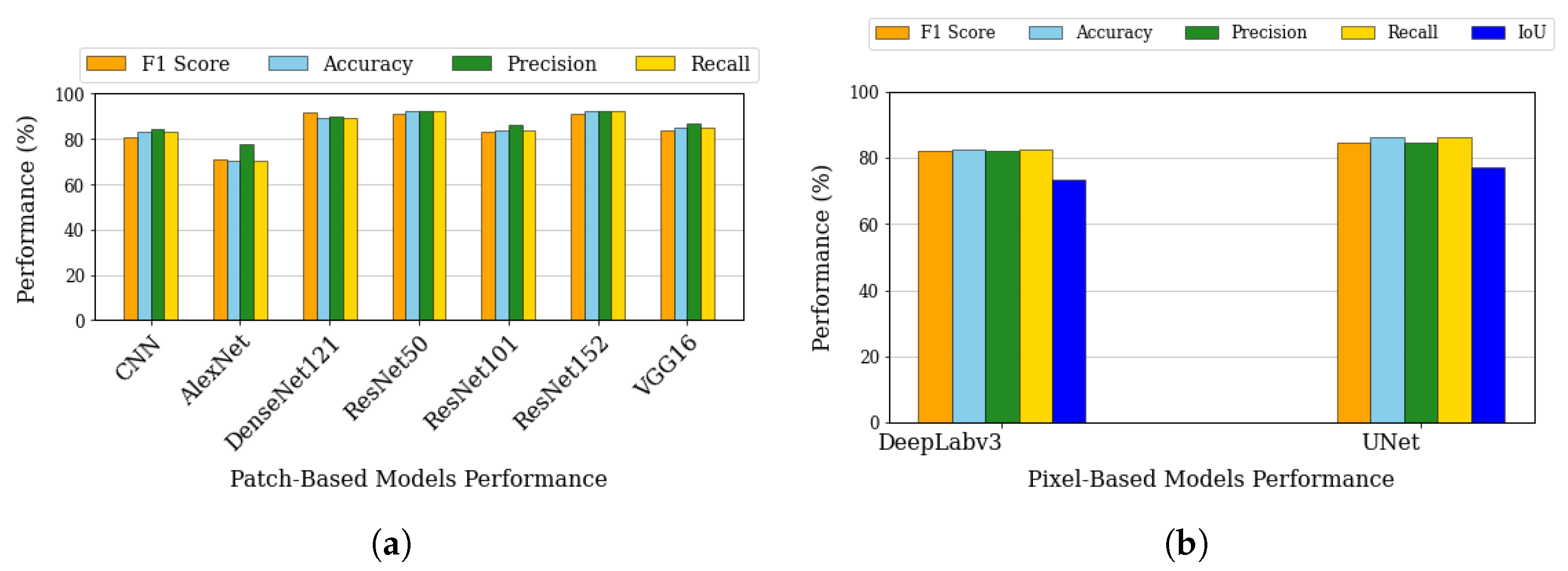
We conducted a comprehensive evaluation of models within the IceBench framework. Our evaluation began with a systematic assessment of all models using standardized metrics and testing protocols. For each model, we computed accuracy metrics as well as computational efficiency metrics. We identified the top-performing models within each classification category based on the F1-score metric. The final phase of our analysis involved a thorough comparison between the leading models from both approaches, examining their relative strengths, limitations, and performance trade-offs.

Beginning with patch-based classification, our analysis encompassed various architectures as shown in Figure 4a. DenseNet121 achieves the highest F1-score at 91.57%, while ResNet152 demonstrates a very similar F1-score. Meanwhile, ResNet50 and ResNet152 achieve the highest accuracy at 92.22%. While these metrics are significantly better than simpler architectures like AlexNet (F1: 70.87%) and basic CNN (F1: 80.53%), VGG16 falls behind the top performers like DenseNet121 and ResNet variants. This middling performance could be attributed to VGG16’s relatively simple architecture that uses repeated blocks of convolutional layers with small filters. While this design is effective for many computer vision tasks, it lacks advanced features like skip connections (ResNet) or dense connectivity (DenseNet) that help modern architectures achieve superior performance in complex tasks like sea-ice classification. When training DenseNet121 from scratch instead of using ImageNet weights [61], the F1-score dropped significantly to 78.29%, highlighting the advantage of transfer learning. Based on these compelling results, we selected DenseNet121 with ImageNet pre-trained weights (hereafter referred to simply as DenseNet) as our top-performing patch-based model [62].

Similarly, for the pixel-based segmentation approach, we focused on pixel-based classification architectures, specifically evaluating U-Net and DeepLabV3 models. As shown in Figure 4b, U-Net achieves higher scores in F1 (84.78% vs. 82.00%), accuracy (86.36% vs. 82.70%), precision (84.68% vs. 82.17%), recall (86.36% vs. 82.70%), and IoU (77.18% vs. 73.51%). U-Net’s better performance can be attributed to its symmetric encoder–decoder architecture with skip connections, which is particularly effective for sea-ice pixel-based classification as it preserves both fine-grained spatial details and global context information. The skip connections allow the network to maintain high-resolution features from the encoder path, which is crucial for accurate ice-type boundary delineation. While DeepLabv3 also shows solid performance above 80% in most metrics, its slightly lower performance might be due to its atrous convolution approach, which, although effective for general pixel-base classification, may not be as optimal for capturing the specific texture and boundary patterns characteristic of different sea-ice types. Both models achieve relatively high IoU scores (over 70%), indicating good overlap between predicted and ground truth segmentations, with U-Net’s higher IoU of 77.18% suggesting more precise boundary predictions.

This architectural distinction mirrors the dual challenges in sea-ice analysis: broad-scale pattern recognition for identifying ice regimes versus precise delineation of boundaries between ice types. Patch-based approaches excel at capturing the distributed patterns and textural signatures that characterize homogeneous ice areas—similar to how human ice analysts first assess the general impression of an ice scene before detailed analysis. DenseNet’s dense connectivity fosters extensive feature reuse and smooth gradient flow, which together boost patch-level ice-type classification accuracy. Meanwhile, pixel-based models demonstrate superior performance in boundary regions where fine-grained transitions occur. This advantage stems from their encoder–decoder architecture with skip connections preserving spatial precision—analogous to how ice analysts conduct detailed edge tracing after initial characterization. The superior performance metrics in precision and IoU metrics for U-Net specifically highlight its strength in accurate boundary delineation.

While our accuracy metrics provided insights into classification capabilities, we complemented this with efficiency metrics focused on practical deployment considerations.

Table 5. Comparison of Model Efficiency Metrics for Pixel-based and Patch-based Models.

Model	Training Phase					Inference Phase
	AvgMT (GB)	MaxMT (GB)	TotCT (Hrs)	AvgET (Min)	TotTT (Hrs)	AvgMI (GB)	MaxMI (GB)	TotCI (Hrs)	TotTI (Min)
Pixel-based Models
U-Net	2.3	3.4	38.3	4.6	7.2	3.8	4.1	0.03	4.4
DeepLabv3	2.2	3.3	27.5	4.6	5.5	3.7	4.1	0.03	4.0
Patch-based Models
CNN	4.1	5.1	13.8	12.3	6.5	4.9	4.9	0.01	0.71
AlexNet	5.0	5.2	15.7	12.3	7.1	5.0	5.0	0.01	0.70
DenseNet121	4.2	4.4	17.9	12.6	7.2	4.9	4.9	0.01	0.73
ResNet50	5.1	5.5	15.1	12.4	6.3	4.9	4.9	0.01	0.74
ResNet101	4.3	5.1	18.6	12.5	7.4	5.0	5.0	0.01	0.74
ResNet152	4.3	5.2	17.4	12.4	6.3	5.0	5.0	0.01	0.75
VGG16	3.8	5.9	19.0	12.4	7.5	4.6	4.6	0.01	0.73

presents these efficiency metrics across all models, with values reported as averages over multiple runs. These two approaches exhibit distinct computational footprints, driven by how each method processes images, their respective epoch lengths, and overall convergence pattern. Resource utilization patterns reveal notable trends across approaches, leveraging 48 CPUs and 1 GPU for both training and inference.

Pixel-based models require higher core-hour consumption due to slower training convergence and full-resolution image processing during validation and inference. Their smaller epoch length enables each epoch to process less data, resulting in lower memory usage per training step and faster per-epoch computation. However, they require more epochs to achieve convergence during training compared to patch-based models, leading to substantially longer total computation times (27.5–38.3 h) than their patch-based counterparts (13.8–19.0 h). Additionally, their computationally intensive inference phase results in longer inference times of approximately four minutes due to their decoder-heavy architecture, which upsamples feature maps back to the original image resolution. While both patch-based and pixel-based models apply convolution operations over all pixels, pixel-based models typically include additional decoder stages, which increase computational complexity and memory usage during inference. In contrast, patch-based models flatten feature maps and apply a fully connected layer for region-level classification, enabling faster inference. During training, patch-based models exhibit higher memory consumption and significantly longer epoch durations due to their larger epoch length, which is five times larger compared to pixel-based models. As a result, these models have a longer epoch duration (about 12 min per epoch) and a greater number of iterations, with total training times ranging from approximately 6.3 to 7.5 h. Additionally, the smaller fixed patch size used during inference facilitates considerably faster inference (around 0.7 min total), as fewer data are processed at once. Among the patch-based models, the ResNet family exhibits similar performance profiles with minimal differences in computational efficiency. DenseNet offers a balanced performance profile with moderate memory usage during training. However, VGG16 records the highest memory spike during training, making it less ideal for resource-constrained environments. Overall, pixel-based models preserve spatial relationships but are computationally intensive, while patch-based models offer faster inference, making them ideal for real-time applications. The choice depends on priorities: training efficiency, inference speed, or memory constraints.

Based on the accuracy metrics, we identified U-Net and DenseNet as the top performers in pixel-based and patch-based categories, respectively. The key challenge in this comparison arises from their distinct classification granularities: U-Net generates pixel-wise predictions, while DenseNet assigns a single classification to entire patches. To ensure a fair comparison between these two models, we established a uniform evaluation methodology using pixel-level ground truth as the reference standard. Test images were processed by both model types, and the DenseNet’s predictions were mapped back to the pixel level to align with the ground truth for direct comparison.

Table 6. Comparative Performance Metrics of U-Net and DenseNet for Fair Evaluation.

Model	F1-Score	Accuracy	Precision	Recall	IoU
U-Net	84.78	86.36	84.68	86.36	77.18
Densenet121	53.89	54.77	63.79	54.77	38.51

presents these comparative results, revealing a significant performance disparity. The DenseNet showed markedly lower performance metrics when evaluated against pixel-level ground truth, primarily due to its inability to handle mixed-label scenarios. When patches contain pixels from multiple ice classes, a common occurrence in real-world sea-ice imagery, the model must make a single classification decision for the entire patch, inevitably compromising pixel-level accuracy.

This direct comparison between the leading models yields crucial insights into the practical implications of model selection for sea-ice type-classification tasks. While patch-based approaches offer computational efficiency and good performance for homogeneous regions, their accuracy decreases significantly when precise pixel-level classifications are required, particularly in areas with diverse ice types. These findings underscore the importance of aligning model selection with specific application requirements—choosing pixel-based approaches for applications requiring high spatial precision and patch-based approaches for scenarios where computational efficiency and broader ice type characterization are prioritized.

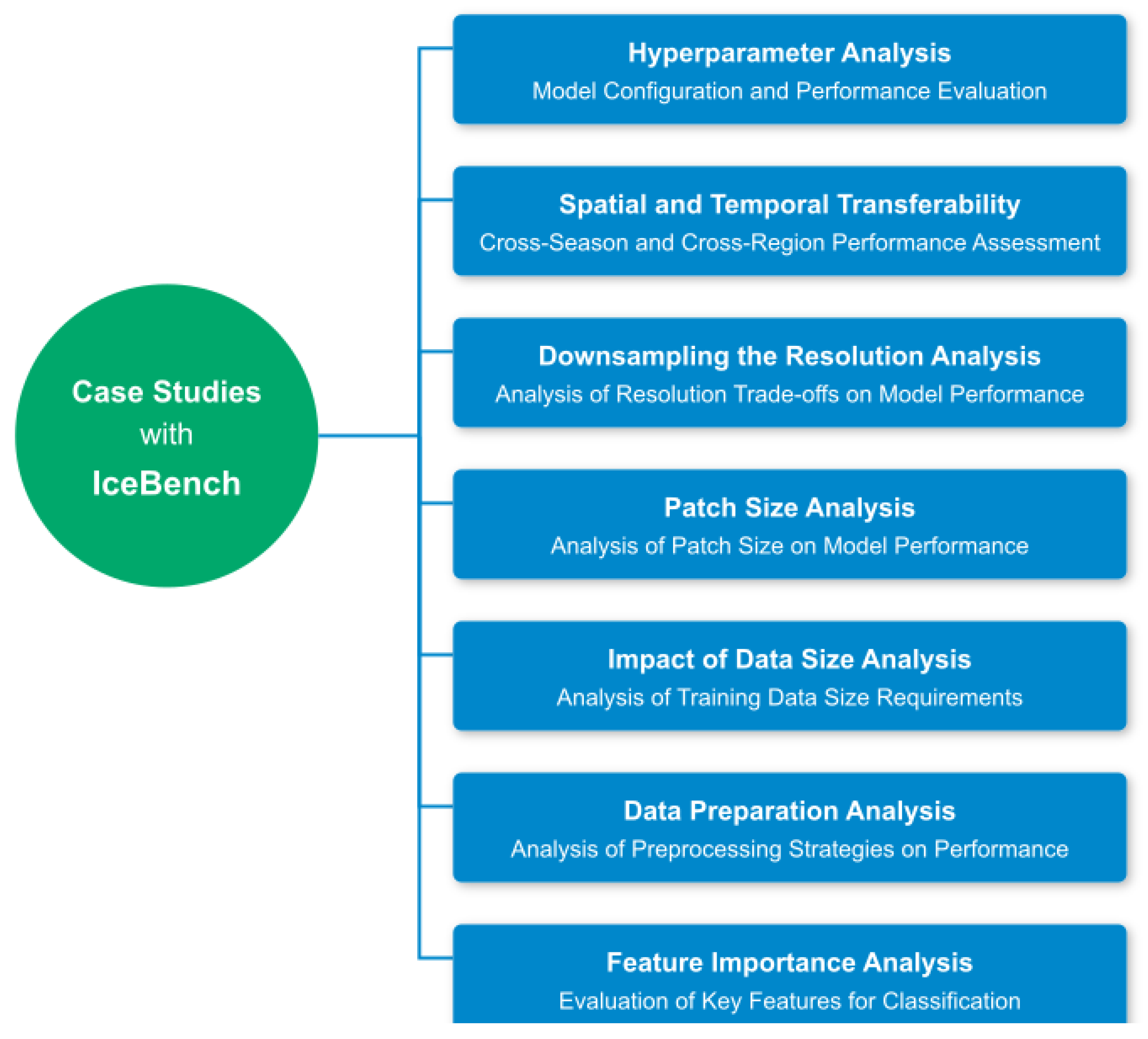
5. Case Studies with IceBench

Understanding the sensitivity of sea-ice type-classification models to various parameters is essential for building robust, operational systems. Therefore, in this section, we use IceBench to investigate critical factors influencing model performance in real-world scenarios. Figure 5 outlines the key research questions that guide our analysis.

Toward this end, we addressed six key research questions:

• How well do the models generalize across different temporal and spatial domains? We evaluate the models’ ability to transfer knowledge to unseen seasons and geographical areas.
• What is the optimal balance between spatial context and computational efficiency? We investigate the impact of image downsampling ratios on model performance.
• How does patch size affect model performance? We analyze the trade-offs between patch dimensions and computational resources.
• What is the minimum training data size needed for robust performance? We examine the relationship between dataset volume and model accuracy.
• How do different data preparation strategies affect model performance? We assess the impact of preprocessing approaches and land masking methods.
• Which input channels are most critical for classification accuracy? We identify the most influential spectral and auxiliary channels for effective classification.

Before addressing our research questions in these case studies, we first validated the effectiveness of our hyperparameter optimization process to ensure that the model configurations are well-calibrated and provide a reliable baseline for subsequent analyses. Our investigation encompassed both classification approaches, focusing on key parameters that significantly influence model performance: learning rate, batch size, optimizer choice, scheduler configuration, and the number of U-Net layers.

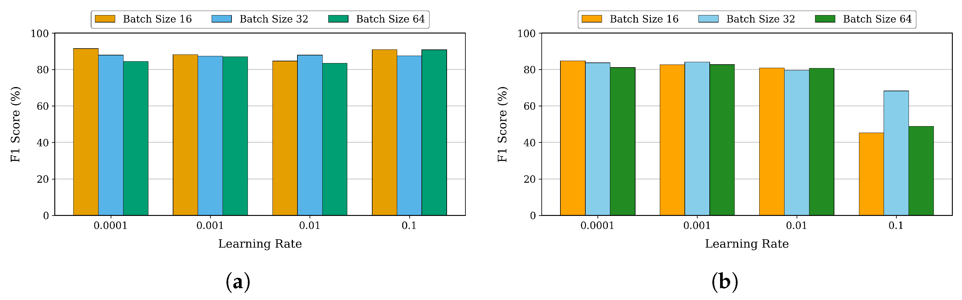
Our initial experiment focused on two key hyperparameters: learning rate and batch size. The learning rate dictates the step size for updating weights, directly influencing convergence speed and stability. Batch size determines the number of samples processed per update, balancing training efficiency and stability.

For DenseNet, we tested different learning rates and batch sizes, as shown in Figure 6a. Using the Adam optimizer with a Reduce-on-Plateau scheduler as our baseline, we tested learning rates from 0.0001 to 0.1 and batch sizes of 16, 32, and 64, evaluating their impact on training performance based on F1-score. At a conservative learning rate of 0.0001, the model demonstrated robust performance across all batch sizes, with batch size 16 showing slightly superior results. When increasing the learning rate to 0.001, we observed a minor degradation in F1-scores across batch sizes, though the model maintained stable performance. Interestingly, at a higher learning rate of 0.1, the model showed remarkable resilience, achieving an F1-score of 91.00% with batch size 16 and even surpassing lower learning rate configurations in accuracy and precision. At this higher learning rate, larger batch sizes also showed promise, with batch size 64 achieving a strong F1-score of 90.85%.

Expanding our analysis to pixel-based segmentation, we conducted a similar evaluation for the U-Net model. Figure 6b presents the F1-scores across different learning rates (0.0001 to 0.1) and batch sizes (16, 32, and 64), using SGD optimizer with a Cosine Annealing scheduler as the baseline configuration. U-net demonstrated distinct behavior patterns across different parameter combinations. At a lower learning rate of 0.0001, we observed consistently superior performance, particularly with a batch size of 16, achieving an F1-score of 84.78%, accuracy of 86.36%, and a Jaccard Index of 77.18%. As we increased the batch size to 64 under this learning rate, the performance showed slight degradation while maintaining overall robustness. When testing higher learning rates of 0.001 and 0.01, the model maintained strong performance, especially with smaller batch sizes of 16 and 32. However, at a learning rate of 0.1, we observed a significant drop in F1-scores across all batch sizes, indicating this learning rate exceeded the optimal range for stable training. Smaller batch sizes, especially batch size 16, consistently achieve higher F1-scores due to better gradient estimates and more frequent updates. In summary, lower learning rates (0.0001 and 0.001) with smaller batch sizes (16 and 32) yield better F1-scores.

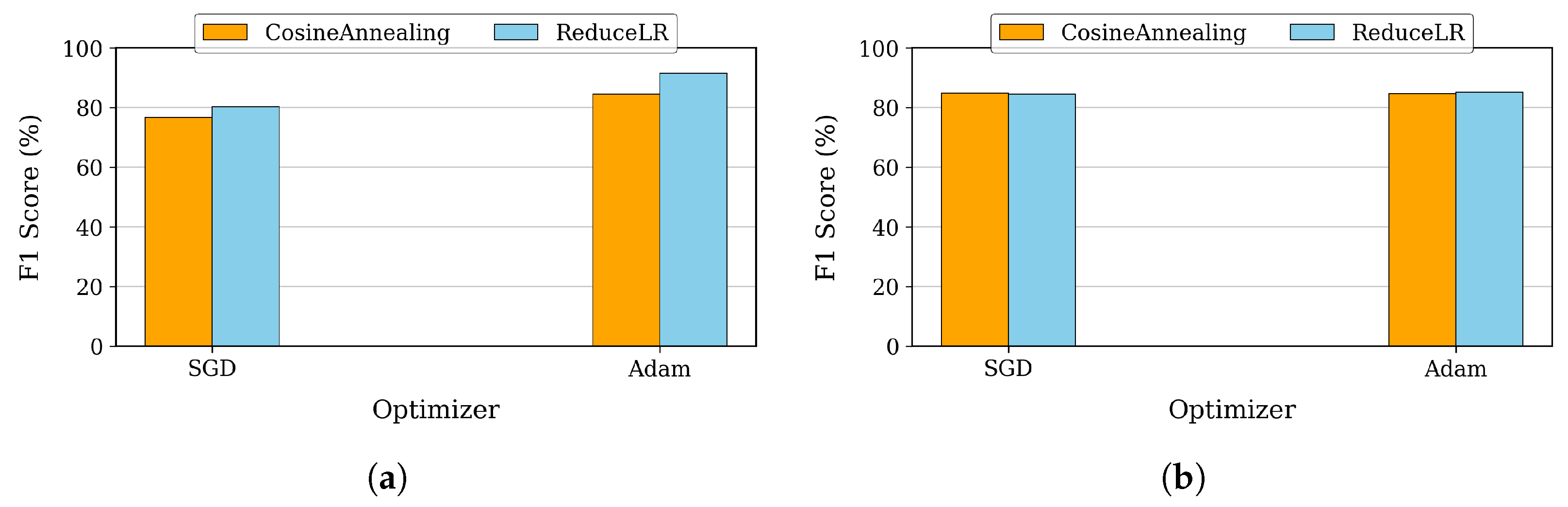
Building on our hyperparameter analysis, we next examined the impact of optimizer choice and scheduler configuration on model performance. These factors play a crucial role in training dynamics—optimizers influence weight updates and convergence speed, while schedulers adjust learning rates to enhance stability and prevent overfitting. For DenseNet, we compared the performance of Adam and SGD optimizers, each paired with either a Reduce-on-Plateau or Cosine Annealing scheduler. Figure 7a illustrates the F1-scores across these configurations, highlighting their effects on training efficiency and classification accuracy. The combination of the Adam optimizer with the Reduce-on-Plateau scheduler emerged as the optimal choice, achieving our highest F1-score of 91.57%. This comprehensive analysis revealed that for patch-based classification, a learning rate of 0.0001 combined with a batch size of 16 provides the best balance for effective learning while demonstrating the model’s robustness across a wide range of parameter settings.

Similarly, for U-Net, we evaluated the impact of optimizer and scheduler selection on segmentation performance. As shown in Figure 7b, we tested SGD and Adam optimizers alongside Cosine Annealing and Reduce-on-Plateau schedulers, analyzing their influence on F1-scores and convergence behavior. The combination of the Adam optimizer with the Reduce-on-Plateau scheduler proved most effective, achieving an F1-score of 85.03% with batch size 16. This superior performance of smaller batch sizes, particularly batch size 16, can be attributed to more frequent model updates and better gradient estimates.

Continuing our investigation, we analyzed the impact of model architecture variations on performance, specifically focusing on the depth of U-Net. Our experiments compared U-Net variants with 4 and 5 encoding/decoding layers. The 5-layer configuration (with layer depths of 32, 32, 64, 64, 128) achieved an F1-score of 82.63%, accuracy of 83.60%, and a Jaccard Index of 73.54%. Interestingly, the 4-layer architecture [32, 32, 64, 64] demonstrated superior performance with an F1-score of 84.78%, accuracy of 86.36%, and a Jaccard Index of 77.18%. This finding suggests that increasing model complexity beyond four layers does not necessarily yield better results for our specific task.

Throughout these experiments, our initial parameter selections consistently demonstrated strong performance, validating our preliminary choices for the sea-ice type-classification task.

5.1. Spatial and Temporal Transferability

In sea-ice monitoring, a model’s ability to generalize across different locations and seasons is essential for practical deployment. This transferability determines whether a model trained on data from one location or season can maintain its performance when applied to another.

We first define the seasons and then group ice monitoring locations based on their ice distribution patterns according to conventional seasons (spring, summer, fall, and winter). Then, in Section 5.1.1, we assess seasonal and spatial transferability by training models on specific conventional seasons and locations and testing them on different ones. In Section 5.1.2, we perform a similar analysis based on cryospheric seasons, evaluating how well the model generalizes across spatial and temporal variations under these ice-specific seasonal phases. To ensure robust validation, we reserved 10% of the training data as a validation set. During training, we select the best-performing model based on the lowest validation loss and then evaluate its performance on test sets drawn from different locations and seasons.

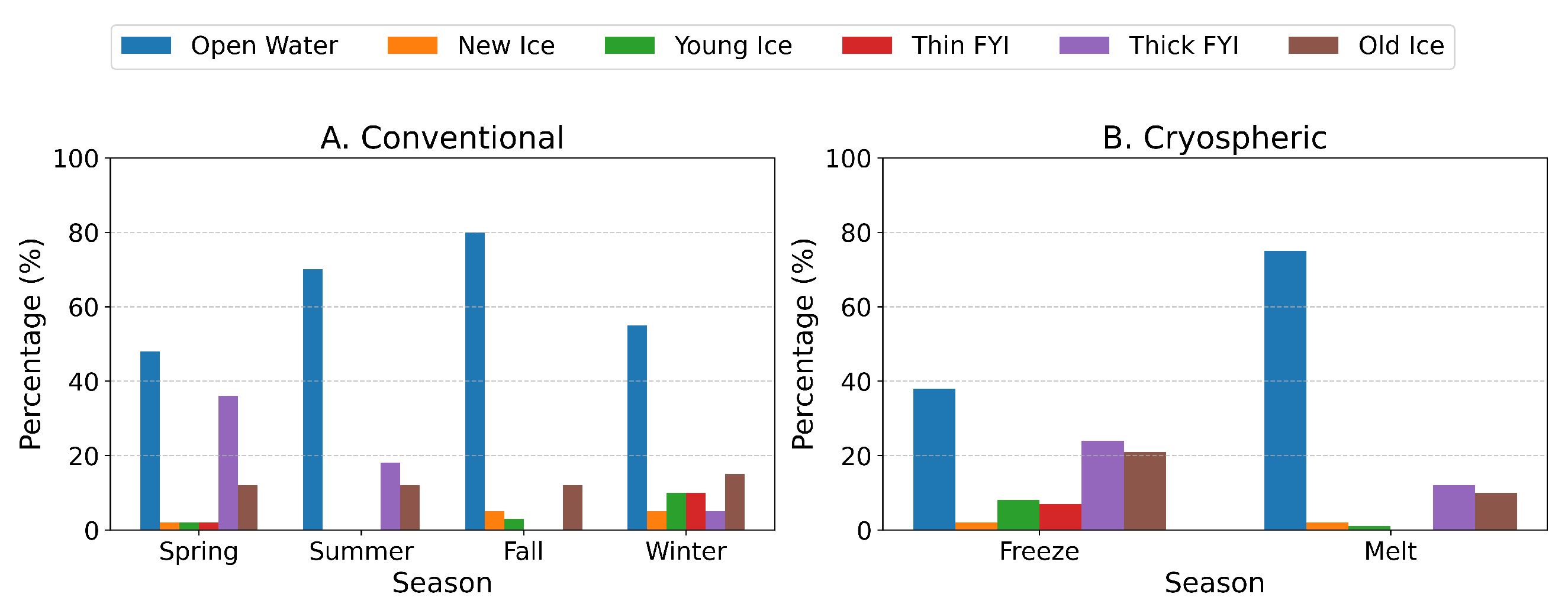
Structuring Seasonal Definitions for Ice Analysis: To capture the complex dynamics of ice conditions, we established two complementary seasonal classification definitions. Our first approach follows the conventional seasonal divisions—spring, summer, fall, and winter. While this categorization provides a familiar structure, it does not fully reflect the key transitions in ice-covered regions, where freeze and melt cycles drive environmental changes more significantly than calendar-based seasons. Recognizing this limitation, we developed a cryospheric seasonal classification, which directly captures the critical phases of ice formation and melting across different regions.

The cryospheric classification system is a more specialized approach and introduces cryospheric seasons that divide the year into melt and freeze periods based on the location’s temperature conditions. This cryospheric classification draws from the Arctic Sea-Ice Melt dataset, which provides crucial information about thermal transitions in sea-ice conditions. These periods are defined using the melt and freeze variables from the Arctic Sea-Ice Melt dataset, which tracks thermal transitions. The melt season captures the period when sea-ice shifts from frozen to melting, while the freeze season marks the return from melting back to frozen conditions. This dataset, part of the NASA Earth Science data collection, consists of daily averaged brightness temperature observations from the Scanning Multichannel Microwave Radiometer (SMMR) and the Special Sensor Microwave/Imager (SSM/I) sensors. The data are mapped onto a 25 km polar stereographic grid, providing high-resolution insights into sea-ice thermal changes. Additionally, the dataset includes yearly maps of key ice phases: early melt (initial signs of melting), melt (sustained melting until freeze begins), early freeze (first observed freezing conditions), and freeze (continuous freezing conditions) [63].

We used Arctic Sea-Ice Melt data with the AI4Arctic Sea Ice Challenge Dataset by mapping where our data overlaps with the Arctic dataset and analyzing how they relate spatially. A conservative definition of the melt and freeze seasons is to use the dataset’s melt and freeze variables, where the melt season spans from melt onset to freeze, and the ice growth season extends from freeze to the following year’s melt. To determine whether a given day falls in the melt or freeze season, we compare the day of the year from our scene files to the Arctic dataset’s average melt and freeze dates. If the day occurs between the average melt date and the average freeze date, it is classified as melt season (264 files). If the day either occurs after the average freeze date or before the average melt date, it is classified as freeze season (212 files). This classification system lets us precisely identify seasonal ice conditions for any given date in our dataset. These definitions allow us to assess how well the model performs under varied environmental conditions, enhancing our understanding of its adaptability and effectiveness in different seasonal contexts.

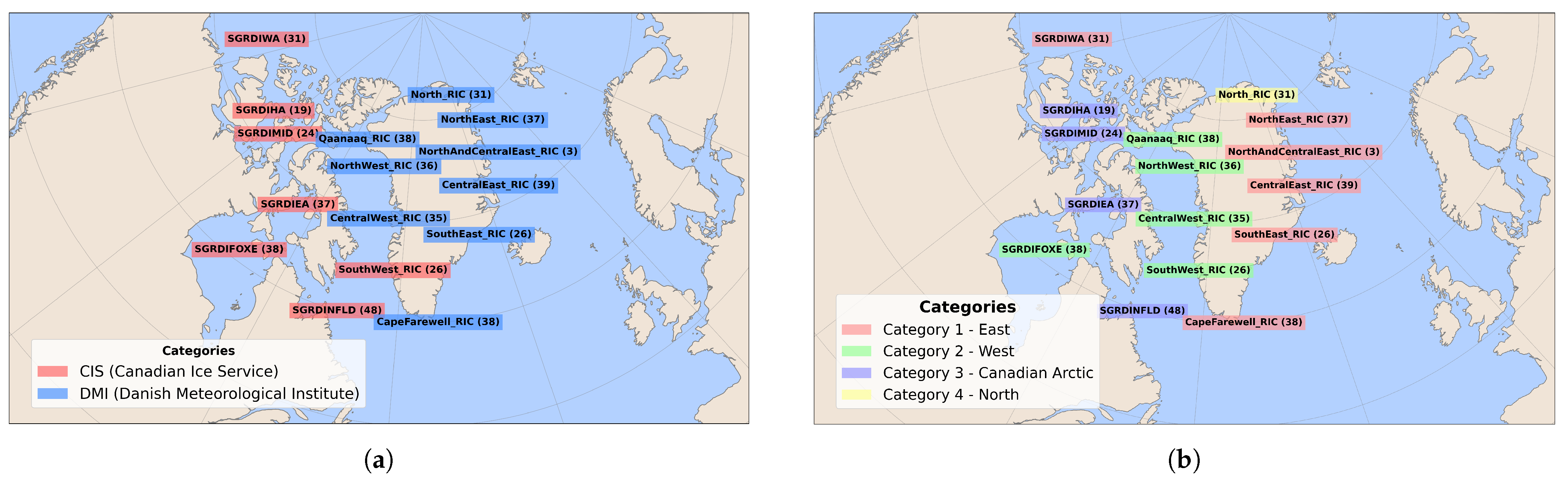
Grouping Ice Regions by Seasonal Behavior: To better understand the model’s generalizability across different locations, we conducted a systematic analysis of regional variations in ice distribution. The dataset includes 16 distinct locations monitored by the CIS and DMI centers from January 2018 to December 2021, as shown in Figure 8a.

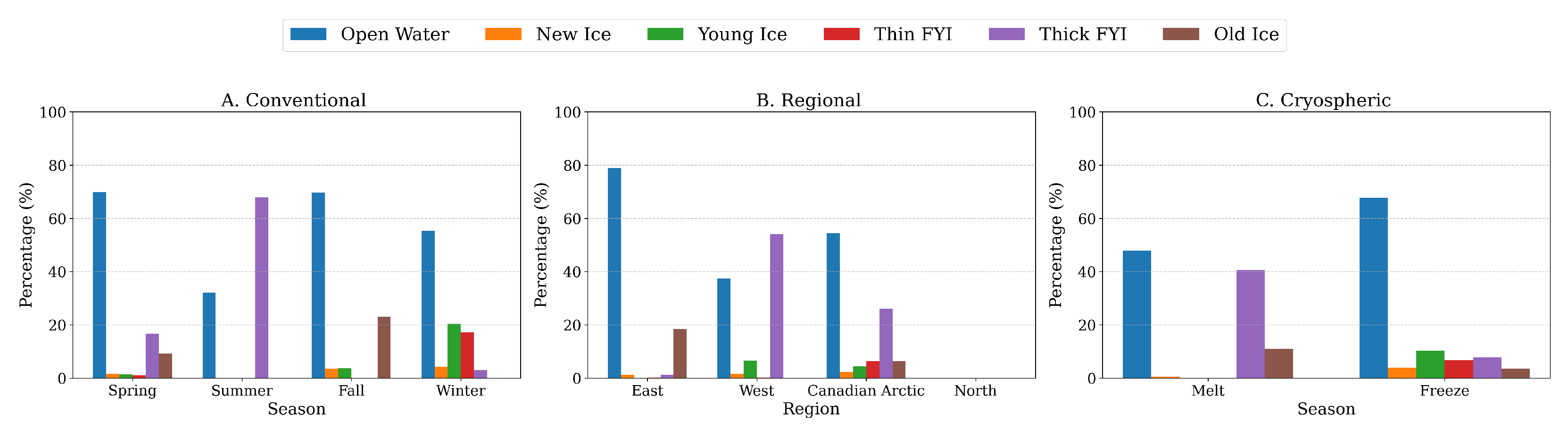
By carefully analyzing how ice classes are distributed across different locations throughout the conventional seasons, we uncovered distinct regional ice patterns. Our approach began by quantifying the percentage of each ice class at every location across all four seasons. This analysis revealed natural groupings among locations based on their seasonal ice behavior, allowing us to classify them into four distinct categories. Figure 8b illustrates this classification, highlighting how ice regions were grouped based on their seasonal ice distribution patterns. To further examine these groups, Figure 9 provides a detailed visualization of the seasonal ice type distribution within each category, offering a comprehensive comparison of ice characteristics across different regions.

These categories, primarily defined by their geographic locations, exhibit markedly different seasonal patterns in ice evolution. The Eastern region (Category 1) demonstrates persistent Open water and Old ice throughout the year, with notable seasonal fluctuations in Thick First-Year Ice (FYI) while maintaining relatively stable ice class proportions. The Western region (Category 2) shows clearer seasonal transitions, dominated by thick FYI during spring, shifting to predominantly Open water in summer and fall, with diverse ice distribution in winter months. Moving to the Canadian region (Category 3), we observe a consistent Open-water presence year-round, complemented by seasonal variations where thick FYI becomes predominant in spring and summer, Young ice prevails in winter, and New Ice forms during fall. The Northern region (Category 4) is distinguished by its substantial Old ice presence, with seasonal shifts showing increased Open water during fall and winter and higher concentrations of thick FYI in spring and summer.

These distinct seasonal distribution patterns across categories provide crucial insights into the regional characteristics of sea-ice behavior and evolution throughout the year.

5.1.1. Transferability Across Conventional Seasons and Geographic Regions

To evaluate the model’s ability to generalize across different conventional seasons and geographic regions, we designed two sets of experiments. The first experiment focuses on seasonal transferability, where the model is trained on data from a specific conventional season and then tested on different conventional seasons within the test dataset. The second experiment examines geographic transferability, where the model is trained on data from a specific geographic location and tested on different categorized locations in the test dataset. These categories correspond to the four regional groupings we previously defined.

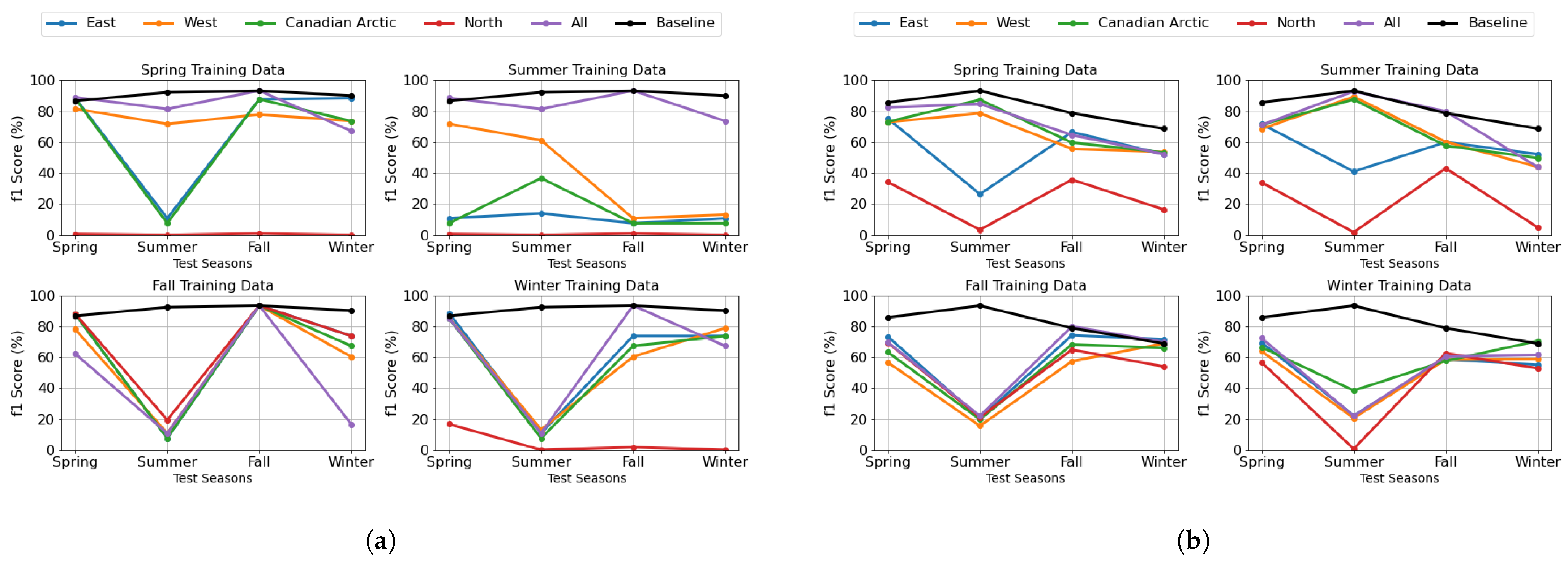
We began our season transferability analysis by investigating how models perform when trained on a specific conventional season and tested across conventional seasons while also accounting for geographic variations. Figure 10a,b provide a comprehensive visualization of this interaction between seasonal and geographic factors for the DenseNet and U-Net models, respectively. These plots show how well each season-specific model generalizes to the other seasons, providing an overall view of how sensitive the system is to shifts in seasonal conditions. Each subplot in the figures represents a model trained on a specific conventional season, as indicated in the title of the plot. The x-axis shows test seasons; the y-axis shows the F1-score (%) for model performance. Each colored line represents one of the four regional groups, illustrating how the model trained on a specific season performs when applied to different geographic locations. The “All” category includes all regions, meaning the model was trained on a particular season regardless of location. The “Baseline” category, shown in the legend, represents a model trained on all locations and all seasons, serving as a reference for overall performance comparison.

Model performance heavily depends on the seasonal class distribution between training and testing data. Figure 9 and Figure 11A show the differences in ice class distributions between the training and test data. Models excel when tested during their training season but struggle with off-season scenarios due to distribution mismatches. The performance drops occur because models adapt to specific seasonal ice conditions and struggle with underrepresented features. A baseline model trained on diverse data from all seasons and locations achieves more consistent cross-scenario performance, highlighting the importance of diverse training data for robust generalization. Winter and summer test data pose challenges due to their ice compositions. Winter has more young and new ice, while summer contains thicker FYI, both of which are harder to classify. Models trained in other seasons struggle due to limited exposure to these ice types. Regional variations further impact model generalization: Canadian Arctic and West show stable results in spring and summer, benefiting from a more balanced mix of ice types. The thick FYI observed in the test data during these seasons primarily originates from the Canadian Arctic and the West. North has high variability but performs well when trained on fall, as its train data contains more open water. It also does well on spring test data, which has thick FYI, aligning with its training conditions. East is performing poorly on summer tests due to a low percentage of thick FYI in its training data. The models trained on different regions in fall and winter perform the worst on summer test data because the training lacks enough thick FYI. However, the Canadian Arctic model trained in winter performs slightly better in summer due to some exposure to thick FYI during training.

In this analysis, we focus on the purple line (“All”) in each subplot, which represents a model trained using data from all categorized locations while being specific to the season indicated in the subplot title. This allows us to evaluate how well a model trained on a particular conventional season generalizes when tested across different seasons, providing insight into the temporal transferability of the model. The U-Net and DenseNet models perform best when trained on summer, followed by spring, while winter training results in the lowest performance. Figure 11A and Figure 12A illustrate the seasonal distribution of ice classes in the train and test data. These distributions reveal that spring and summer share similar class distributions, dominated by open water, thick FYI, and old ice, explaining their similar performance levels. The observed temporal transferability patterns, where models trained on transitional seasons (spring and summer) demonstrate better cross-seasonal performance, highlight the importance of capturing ice in various evolutionary stages. These transitional periods encompass both stable ice conditions and dynamic change processes, providing models with exposure to the full continuum of ice states rather than just the extremes of winter formation or summer melt. Spring-trained model: Performs well on spring and summer since the training data contains a large proportion of thick FYI and open water, which are also dominant in spring and summer test data. However, it struggles on winter due to the presence of young ice, which is less represented in the training set. Summer-trained model: Achieves its best performance on summer, followed by spring, due to the high proportion of thick FYI and open water in both seasons. Performance drops in winter, as it lacks sufficient exposure to young ice during training. Fall-trained model: Performs best on fall and spring, as the class distribution in these test seasons closely aligns with the fall training data. However, it struggles in winter, where young ice is dominant, and in summer, which has a large portion of thick FYI, making generalization difficult. Winter-trained model: Surprisingly, achieves its highest performance on spring, likely due to similar class distributions between winter training data and spring in the test, which are thick FYI and old ice. Performance on fall is also reasonable, but it struggles with summer, which contains a significant proportion of thick FYI, a condition it has not encountered as frequently in training. In general, models trained in spring and summer demonstrate moderate generalizability and perform well in seasons with similar class distributions.

After analyzing seasonal transferability, we examined geographic transferability by training models on specific categorized locations and evaluating their performance across different regional groups. Figure 13a,b visualize this analysis for the DenseNet and U-Net models, respectively. Each subplot reflects a model trained on a specific location (title), tested across regions (x-axis) with F1-score (%) on the y-axis. Colored lines indicate training seasons. “Fourseason” models use all seasons; “Baseline” models use all locations and seasons. Note: test dataset does not contain any files from the North location, and therefore, this category is not represented in the results. Figure 9 and Figure 11B show the differences in ice class distributions between the training and test sets.

The patch-based model, as shown in Figure 13a, exhibits regional specificity in its performance. Models trained on data from specific regions achieve optimal performance when tested on data from the same region but show degradation when applied to different regions. The East test location emerges as a particularly interesting case, demonstrating consistently robust performance across different training scenarios, suggesting regional characteristics that facilitate better model generalization. However, when tested on West and Canadian Arctic locations, performance declines notably. The West test location shows the strongest performance with West-specific training data, highlighting effective within-region generalization. The moderate generalization capability of models trained on West regions compared to other regions reveals important insights about Arctic sea-ice dynamics. This enhanced transferability likely stems from the region’s exposure to diverse oceanographic and atmospheric conditions. The region effectively captures a wider spectrum of ice formation, deformation, and melting processes. The pixel-based U-Net model demonstrates different geographic adaptation patterns, as illustrated in Figure 13b. The East test region maintains superior performance regardless of training location, indicating robust feature characteristics in this region. West-trained models achieve optimal results within their home region, matching East region performance levels, but struggle with Canadian Arctic data. Notably, this strong home-region performance shows seasonal variation, with deterioration during fall and winter seasons. Models trained on Canadian Arctic data show good performance in East regions, while North-trained models perform best in East regions and demonstrate moderate success in Canadian regions compared to their West region performance.

The architectural differences between U-Net and DenseNet significantly contribute to their distinct adaptation patterns across different spatial and temporal domains. U-Net’s encoder–decoder structure with skip connections is specifically designed for precise pixel-level segmentation, allowing it to preserve fine-grained spatial details while maintaining global context. This architecture enables U-Net to better handle variations within images and adapt more consistently to unseen conditions. When exposed to novel environmental conditions, U-Net’s skip connections help maintain critical low-level feature information throughout the network, providing resilience when adapting to new ice formations or seasonal transitions. In contrast, DenseNet’s strength lies in its dense connectivity pattern, where each layer receives feature maps from all preceding layers. While this dense feature reuse creates powerful hierarchical representations ideal for patch-based classification, it prioritizes feature abstraction over spatial precision.

5.1.2. Transferability Across Cryospheric Seasons and Geographic Regions

Expanding our analysis from conventional seasons to cryospheric seasons, we conducted the same set of experiments as defined for conventional season transferability but instead used melt and freeze periods. These experiments reveal distinct patterns in both DenseNet and U-Net models, providing insight into their ability to generalize across seasonal transitions and geographic regions in the context of cryospheric seasons.

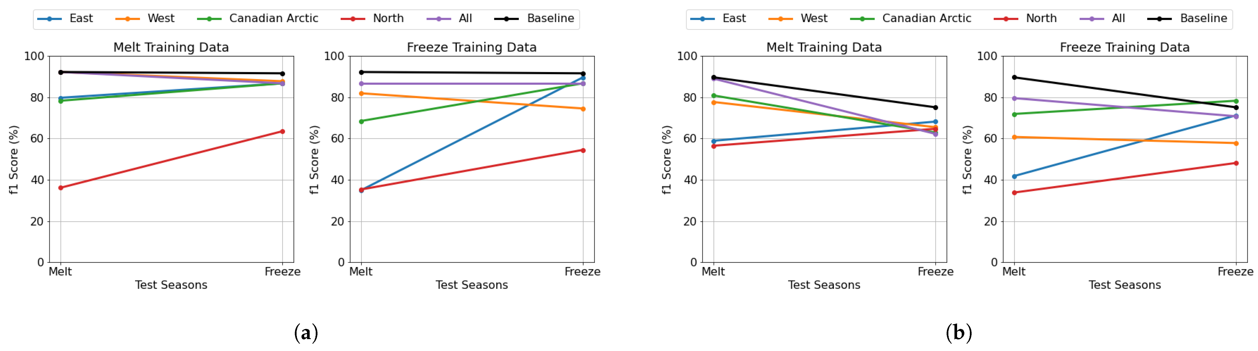
For the seasonal transferability experiment using cryospheric seasons, we evaluated how well models trained on one cryospheric season (melt or freeze) perform when tested on the other. Figure 14a presents the DenseNet model’s performance, while Figure 14b shows corresponding results for the U-Net model. Each subplot represents a model trained on a melt or freezes cryospheric season, while the x-axis denotes the test cryospheric season and the y-axis indicates the F1-score (%). Each colored line corresponds to a specific categorized location. Additionally, two reference categories are included: “All” (purple) represents a model trained on data from all categorized locations within a specific cryospheric season, and “Baseline” (black) represents a model trained on all locations and both cryospheric seasons, serving as a general performance reference.

The patch-based model demonstrates varying transferability patterns across cryospheric seasons. When trained on melt data, the model maintains robust F1-scores (79–90%) for East, West, and Canadian Arctic regions across both test seasons. Interestingly, the North region exhibits an unexpected improvement from 30% during melt testing to 65% during freeze testing. This enhanced performance during freeze testing can be attributed to the higher proportion of open water in freeze test files, which typically presents a simpler classification task. Conversely, the more complex mix of open water and thick FYI in melt test data creates a more challenging classification scenario. Models trained on freeze data show different adaptation patterns. The East, Canadian Arctic, and North regions demonstrate significant improvement from melt-to-freeze testing periods. The West region maintains relatively stable performance across both test seasons. Notably, the baseline performance remains consistently high across both training scenarios, indicating robust overall generalization. The pixel-based U-Net model exhibits distinct regional patterns compared to the DenseNet approach. Under melt data training, the West, Canadian Arctic, and all regions show a gradual decline in performance from melt-to-freeze test seasons, while the East and North regions maintain more stable performance with slight improvements. For freeze training data, the East region shows dramatic improvement when tested across seasons, while the West maintains stable performance throughout. The Canadian Arctic consistently achieves the highest scores, though the North region remains challenging.

In this analysis, we conduct a temporal evaluation by examining the purple line (“All”) in each subplot, which represents a model trained on data from all categorized locations while being specific to the cryospheric season indicated in the subplot title. This allows us to assess the model’s ability to generalize across melt and freeze periods, providing insights into its seasonal transferability. To better understand how seasonal variations impact model performance, we analyze the distribution of ice classes across melt and freeze periods, as shown in Figure 12B for the train and Figure 11C for test. These class distributions highlight key differences in ice conditions between seasons, which directly affect model adaptability. The patch-based classification model demonstrates strong seasonal stability, maintaining consistent performance in both melt and freeze periods. This stability is further enhanced when the model is trained on data that combines both seasons, suggesting that patch-level features remain relatively stable across cryospheric transitions. In contrast, the pixel-based model exhibits seasonal sensitivity. When trained on melt or freeze season data, the model’s performance drops when tested on freeze season. Specifically, training on melt data and testing under melt conditions yields nearly 90% F1-score, but the performance declines to around 62% when tested under freeze conditions. Similarly, training on freeze data achieves approximately 79% F1-score when tested under melt conditions and about 71% F1-score when tested under freeze conditions. Furthermore, as shown in Figure 11C, the classes of new ice and young ice are significantly less present in the melt test data, making it easier for the model to achieve higher performance on melt season predictions. These ice types are particularly challenging for the model due to their variability and transitional nature, which makes their lower prevalence in the melt season beneficial for model accuracy. The increased presence of new and young ice in the freeze test data likely contributes to the performance drop, as these classes introduce more complexity in the classification process.

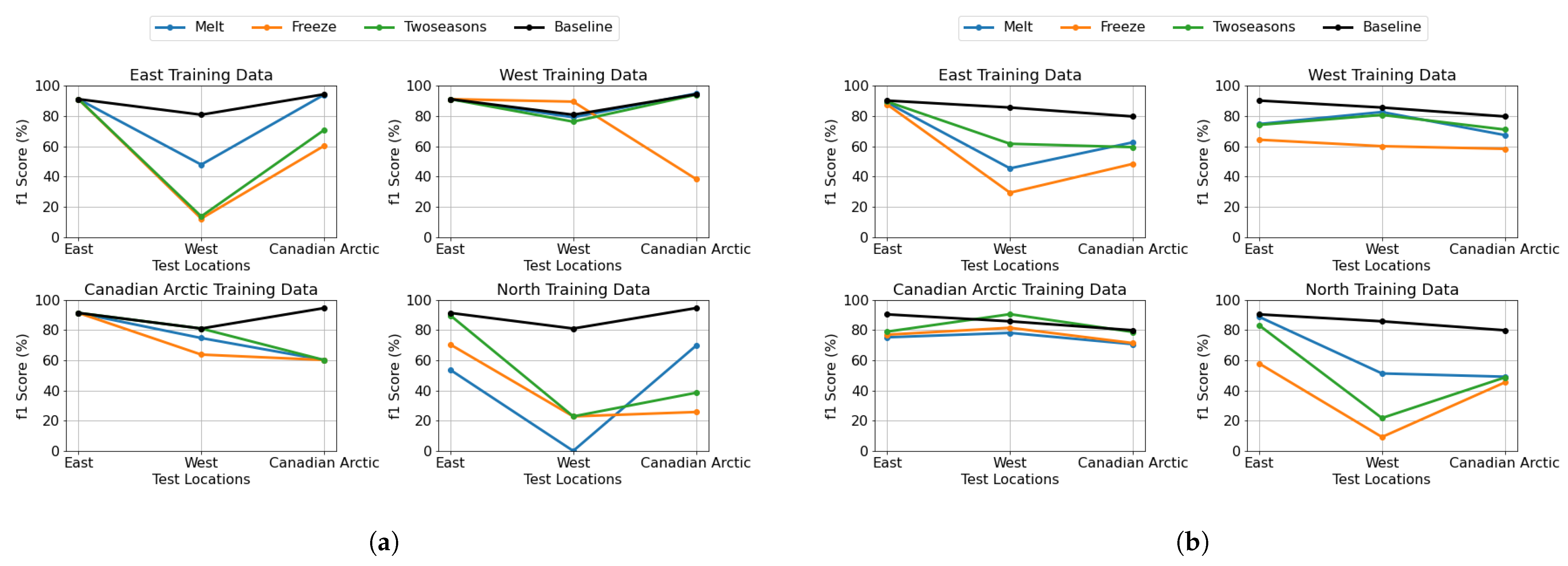
Our analysis of geographic transferability under cryospheric seasonal conditions examines how models trained on specific categorized locations perform when tested on different regional groups during melt and freeze periods. Figure 15a,b illustrate these results for the DenseNet and U-Net models, respectively. Each subplot represents a model trained on a specific categorized location, while the x-axis indicates the test location, showing performance across different regional groups. Each colored line corresponds to a specific cryospheric season melt and freeze, demonstrating how the model trained on one location performs when tested on different regions during each season. The “Twoseasons” category refers to a model trained on both melt and freeze seasons for a specific location. Figure 9 and Figure 11C help illustrate regional ice class distributions.

The pixel-based model shows distinct regional adaptation patterns. The East-trained model achieves impressive F1-scores of approximately 90% on its home region but experiences significant performance degradation (40–60%) when tested on West and Canadian Arctic regions. In contrast, the West-trained model maintains consistent F1-scores between 60 and 80% across all regions, demonstrating strong generalization capabilities. The Canadian Arctic-trained model emerges as the most generalizable, performing exceptionally well on both the East and its home region (80–90% F1-scores) and achieving its best performance on the West region. The North-trained model exhibits high variability, excelling in the East region (80–90% F1-scores) but struggling with the Canadian Arctic and West regions (20–50%). For patch-based classification, we observe different regional adaptation characteristics. The East-trained model demonstrates near-perfect performance in its home region but struggles significantly with the West region while showing improved performance (60–90% F1-scores) on Canadian Arctic data. The West-trained model shows remarkable generalization, excelling not only in its home region but also in East and Canadian Arctic regions, particularly during the melt season. The Canadian Arctic-trained model maintains consistently high performance (60–90% F1-scores) on both East and West regions but, surprisingly, shows lower performance in its home region. The North-trained model achieves high performance (80–100% F1-scores) on East region data but demonstrates poor generalization to West and Canadian Arctic regions (20–40%).

Across both approaches, the West region emerges as the good generalizable, suggesting that it captures a diverse range of characteristics of sea-ice applicable across different regions. East and North regions show similar patterns in both tasks, with models trained on these regions generalizing poorly to other areas but showing some mutual compatibility. Canadian Arctic-trained models demonstrate good generalizability, maintaining moderate performance across East and on West region testing, suggesting they learn features that transfer well across different Arctic environments. The baseline models (trained on all locations and seasons) consistently perform best across all test scenarios, confirming the value of diverse training data. Models trained on two seasons generally outperform single-season models in most regions, indicating the importance of seasonal diversity. Region-specific seasonal patterns are also evident—East-trained patch-based models using melt season data perform better, while North-trained pixel-based models show better performance than the two-season model when trained with melt data.

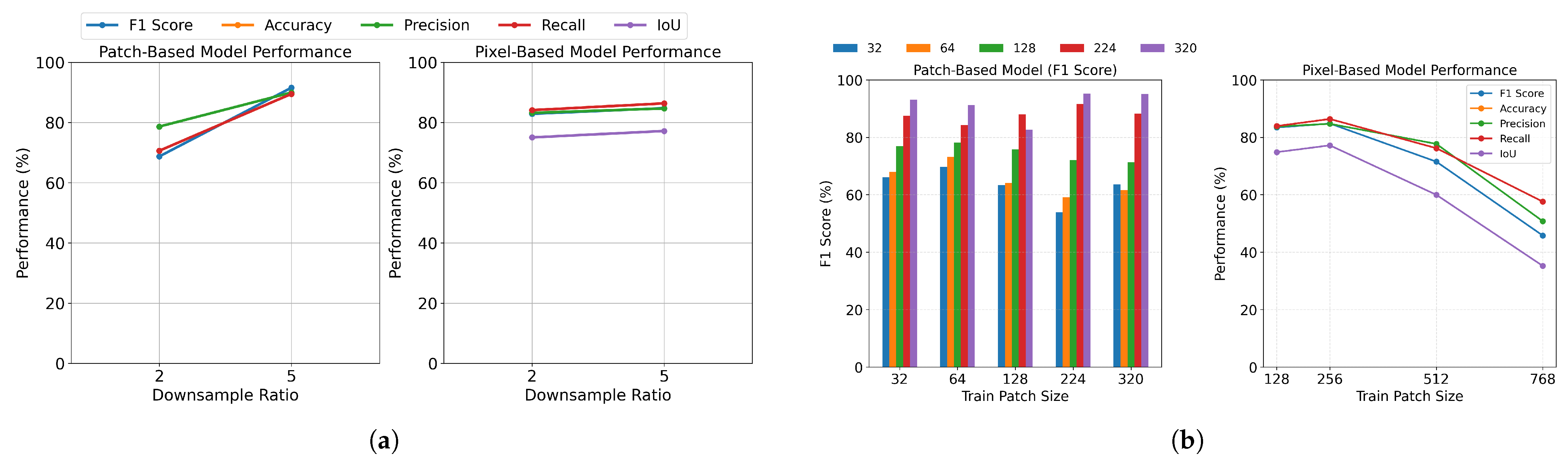
5.2. Exploring the Impact of Downsampling the Resolution

The downsampling ratio of images significantly influences model performance by balancing computational efficiency with detail preservation. While high-resolution scenes contain more detailed information critical for accurate classification in sea-ice monitoring, they demand greater computational resources.

Figure 16a presents two subplots comparing the two models’ performance across different downsampling ratios. The x-axis represents the tested ratios (2 and 5), while the y-axis shows accuracy metrics (%), with each line indicating a different accuracy metric.

Our experimental results demonstrate that for patch-based classification, a downsampling ratio of 5 yielded superior results compared to a ratio of 2. This suggests that moderate resolution reduction does not significantly compromise the model’s ability to identify larger-scale patterns in sea-ice imagery. In pixel-based classification tasks, both downsampling ratios (2 and 5) demonstrated comparable performance, indicating that pixel-level features remain relatively preserved even at lower resolutions. Interestingly, downsampling ratios (2 and 5) demonstrated comparable performance, indicating that pixel-level features remain relatively preserved even at lower resolutions. This may be attributed to the nature of SAR imagery, which often contains speckle noise and high-frequency artifacts. At very high resolutions, speckle noise and micro-variations become more prominent without providing additional discriminative information about ice type. Downsampling effectively acts as a form of noise suppression, smoothing small variations and potentially improving the signal-to-noise ratio in the input features, which can help models focus on broader spatial patterns relevant to ice-type classification.

This performance pattern can be interpreted through the lens of feature preservation versus computational efficiency. While higher resolutions theoretically retain more detailed information, our results suggest that a moderate reduction in resolution can maintain classification accuracy while significantly reducing computational overhead. This finding has practical implications for deploying these models in resource-constrained environments or real-time applications. A notable observation in our study concerns the case of downsampling ratio 1 (original resolution). Despite the theoretical advantage of maximum detail preservation, we had to exclude this configuration from our analysis due to its prohibitive computational requirements. This exclusion highlights the practical limitations that must be considered when deploying deep-learning models in real-world applications.

5.3. Exploring the Impact of Patch Size

Patch size defines the dimensions of sub-images extracted from the larger image, influencing the trade-off between fine-scale detail and broader spatial context. Smaller patches capture intricate ice features but may miss large-scale patterns, while larger patches provide more context but can overlook finer details. To ensure a fair evaluation, we selected patch sizes of 32 to 320 pixels for patch-based models and 128 to 768 pixels for pixel-based models, reflecting common practices in each approach.

Figure 16b presents two subplots comparing pixel-based and patch-based model performance. In the left subplot, the F1-scores of the patch-based model are plotted across five test scenarios, each represented by a different bar color. The plot reveals significant performance patterns across varying training and testing patch sizes for sea-ice classification. The DenseNet model exhibits optimal performance when trained on larger patch sizes (224–320 pixels), achieving F1-score rates exceeding 90%. While all training patch sizes can achieve high performance with larger test patches, the 224-pixel training patch size emerges as particularly effective, yielding the highest F1-score when combined with 320-pixel test patches. Notably, the model trained on larger patches demonstrates superior generalization capabilities across different test patch sizes, suggesting they better capture the contextual information necessary for accurate ice type discrimination. An important observation is the decreasing number of test patches as patch size increases. This reduction in test sample size should be considered when interpreting the results, as it may affect the statistical significance of performance differences. On the right subplot, the pixel-based classification subplot shows optimal performance at a moderate patch size of 256 pixels, with metrics declining for larger patches. As patch sizes increase from 32 to 224 pixels, all evaluation metrics show consistent improvement. This upward trend suggests that patch-based approaches benefit from larger contextual windows, which likely provide richer spatial information for classification decisions. The pixel-based method performs optimally at moderate patch sizes (256 pixels) before declining with larger contexts.

These findings emphasize the critical role of patch size selection in optimizing sea-ice classification models, with larger training patches providing the best balance between feature capture and generalization ability.

5.4. Exploring the Impact of Data Size

Data size is critical for training deep-learning models, particularly for sea-ice classification, where diverse and representative samples enhance generalization. The patch-based model uses pre-generated patches, while for this experiment, the pixel-based model was trained on patches generated with a patch size of 256 and a stride of 100 rather than using random cropping. Figure 17 consists of two subplots, each illustrating the effect of dataset size on the pixel-based and patch-based models. The x-axis represents the number of training samples, while the y-axis shows performance metrics (%), with different lines corresponding to various accuracy measures.

The pixel-based model demonstrates a consistent and gradual learning trajectory. Beginning with minimal effectiveness at small data sizes (50–64 samples), it exhibits steady improvement as the training volume increases. Performance metrics generally plateau after approximately 5000–10,000 samples, indicating the model reaches its learning capacity at this threshold, with additional data offering diminishing returns. A critical insight is that when the data size exceeds 1000 samples, the improvement across all metrics becomes marginal. All evaluation metrics for the pixel-based model follow similar growth patterns. In contrast, the patch-based model achieves strong performance even with limited training data and improves further with larger datasets. This early advantage suggests that the patch-based approach captures relevant features more efficiently. However, its learning curve is more variable, with fluctuations such as an F1-score drops around the 240–320 sample range, possibly due to batch composition effects.

5.5. Exploring the Impact of Data Preparation Methods

Previous studies have demonstrated that variations in preprocessing techniques can significantly influence model generalization, feature extraction, and robustness. Motivated by these findings, we systematically evaluated key data preparation strategies to assess their impact on both patch-based and pixel-based classification tasks. As shown in

Table 7. Classification results of pixel-based and patch-based models with different data preparation strategies.

Scenario	Pixel-Based Model					Patch-Based Model
	F1-score	Accuracy	Precision	Recall	IoU	F1-score	Accuracy	Precision	Recall
With/Without Data Augmentation
With Aug.	84.78	86.36	84.68	86.36	77.18	91.57	89.51	89.97	89.51
Without Aug.	83.44	83.70	84.89	83.70	75.41	81.92	76.54	89.38	76.54
Removing/Including Land Pixels
Remove Land Pixels	83.51	84.35	83.27	84.35	74.73	81.92	76.54	89.38	76.54
Include Land Pixels	84.78	86.36	84.68	86.36	77.18	91.57	89.51	89.97	89.51
Distance to Border (Multiple Thresholds)
Distance to Border (10)	75.02	77.54	79.08	77.54	63.58	70.46	66.05	75.19	66.05
Distance to Border (20)	67.81	72.12	70.78	72.12	55.94	79.27	79.19	87.77	79.19
Distance to Border (40)	69.37	73.96	69.51	73.96	57.14	68.60	63.84	74.92	63.84

, we examined three major data preparation methods: data augmentation, land pixel inclusion, and distance-to-border thresholding. Each technique addresses specific challenges in sea-ice image analysis and contributes to the overall robustness of the classification models.

First and foremost, data augmentation is a widely used technique that artificially increases the diversity of the training dataset by applying transformations such as rotation, flipping, scaling, and cropping. This helps the model generalize better by exposing it to different variations of the data. The results presented in Table 7 for the patch-base model demonstrate its effectiveness for the patch-based model, where data augmentation substantially improved performance, elevating the F1-score from 81.92% to 91.57%. For the pixel-based model, shown in Table 7 for pixel-based, the impact was more modest but still positive, with the F1-score increasing from 83.44% to 84.78%. These improvements indicate that augmentation helps models develop better generalization capabilities by exposing them to diverse ice conditions and mitigating overfitting issues.

Additionally, the consideration of distance to the border represents another technique evaluated for its impact on model performance. The reason for applying a distance-to-border threshold is to reduce label noise introduced by the uncertainty and imprecision in manually drawn ice chart boundaries. As noted in [13], it is challenging for ice analysts to delineate sea-ice regions with pixel-level precision, especially near polygon edges. Border pixels often contain mixed ice types or poorly defined transitions, which can mislead the learning process. This approach aims to increase patch purity by excluding ambiguous regions near class transitions. However, Table 7 shows that the impact of distance-to-border thresholds varies significantly between classification approaches and threshold values. For pixel-based classification, performance consistently deteriorates as the threshold increases, with F1-scores declining from 75.02% at 10 pixels to 67.81% at 20 pixels. This suggests that edge regions provide essential information for accurate pixel-based classification, where precise boundary determination is crucial. For patch-based classification, the relationship is more complex. Performance initially improves from a 10-pixel threshold (F1-score: 70.46%) to a 20-pixel threshold (F1-score: 79.27%), but then degrades dramatically at 40 pixels (F1-score: 68.60%). This non-linear response demonstrates that while the patch-based approach benefits from some boundary noise reduction, excessive exclusion of border regions ultimately removes valuable contextual information necessary for classification. These findings highlight the delicate balance required when applying distance-to-border thresholds and suggest that an optimal threshold exists that may vary by classification approach.

Furthermore, land pixel removal is another technique evaluated for its impact on model performance. By filtering out these pixels, we ensure that the model focuses solely on the relevant sea-ice data. Interestingly, as evident in Table 7, the inclusion of land pixels emerged as a beneficial factor for both classification approaches. In patch-based classification, this inclusion led to a substantial improvement in the F1-score from 81.92% to 91.57%, accompanied by significant enhancements in accuracy and recall. DenseNet’s dense connectivity makes it sensitive to data distribution. Removing land pixels with contextual cues can disrupt feature reuse and degrade performance. The pixel-based classification showed similar benefits, with the F1-score rising from 83.51% to 84.78%. Coastlines represent critical transition zones where ice formation processes differ substantially from open ocean environments. By preserving land pixels, models can learn these coast-proximal patterns and the gradual transitions that occur when moving away from land. Furthermore, the contrast between land and water/ice provides stable reference points that improve the model’s ability to calibrate its classification thresholds across varying illumination and atmospheric conditions. These improvements suggest that land pixels provide valuable contextual information, particularly at coastline interfaces where the distinction between land, water, and ice types is critical.

5.6. Feature Importance Analysis

Understanding how different input features influence model behavior is crucial for both model interpretation and validation in sea-ice classification. Our analysis employs multiple attribution methods to quantify and compare feature importance across both approaches, providing insights into how each model makes decisions across six different ice types.

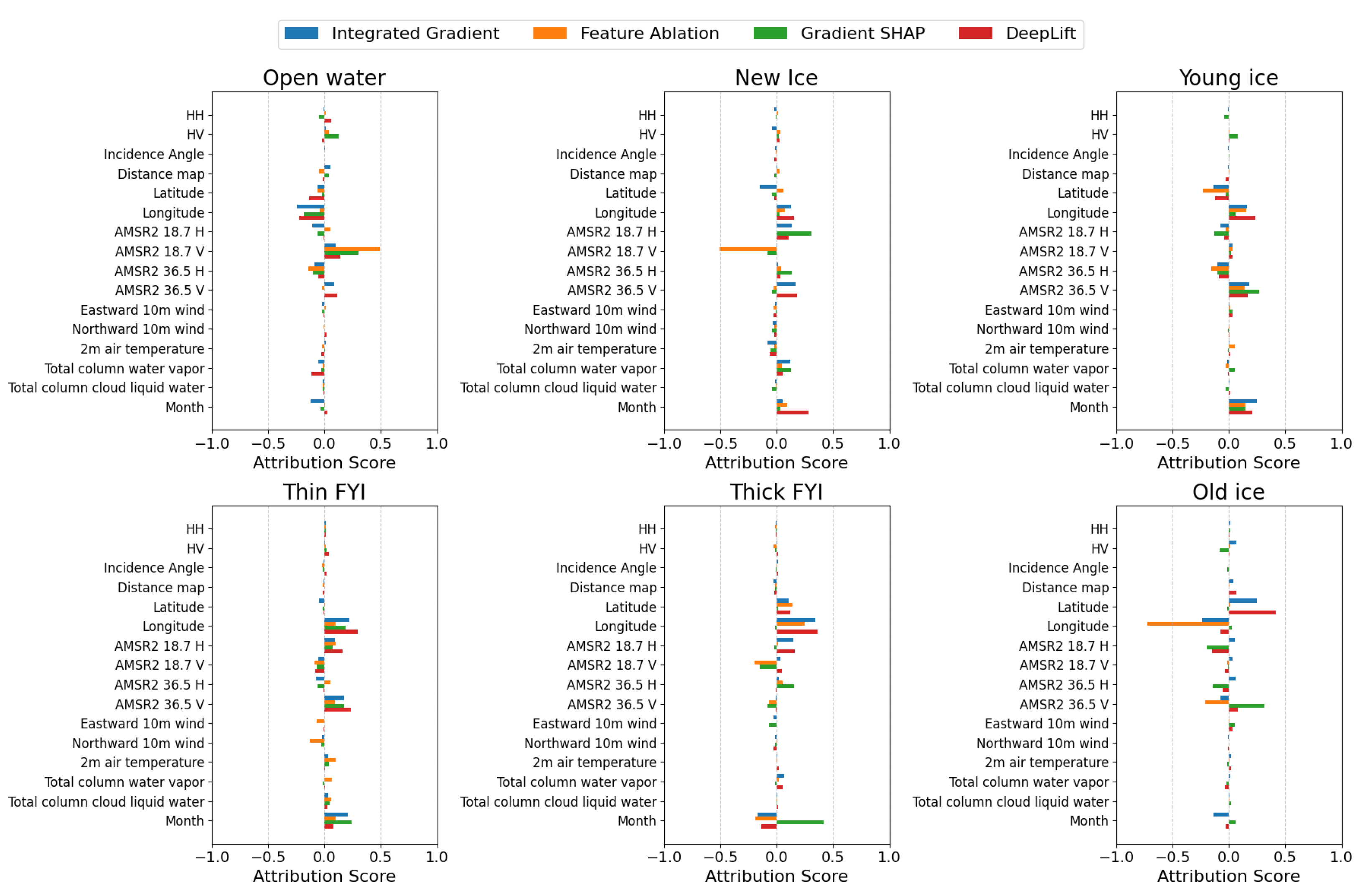
For this investigation, we employed Captum, a comprehensive model interpretability library. The analysis incorporates four attribution methods: Integrated Gradient, which computes attribution by integrating gradients along a specified path from baseline to input; Feature Ablation, which systematically removes features to measure their impact; Gradient SHAP, which applies Shapley values from cooperative game theory; and DeepLift SHAP, which combines Shapley values with the DeepLift framework to assess feature contributions relative to a reference point [64].

The patch-based classification model’s feature importance analysis, shown in Figure 18, reveals distinctive patterns across different ice classes. In the plot, HH and HV stand for the SAR primary (nersc_sar_primary) and SAR secondary (nersc_sar_secondary), respectively.

Longitude emerges as a dominant feature, demonstrating consistently high importance across most ice types. This geographical dependency suggests that spatial location plays a fundamental role in ice type determination. The model exhibits varying reliance on features such as distance maps and temperature metrics, indicating these parameters have specialized relevance for specific ice conditions. Seasonal patterns, captured through the “month” feature, show substantial importance in certain ice classifications, highlighting the temporal dynamics of ice formation and transformation. Temperature-related features and meteorological variables like total column water vapor and liquid water demonstrate varying significance, particularly in identifying thick FYI. Notably, some features display negative attribution scores, indicating that their absence serves as evidence against particular ice classifications, demonstrating the model’s sophisticated decision-making process.

The segmentation model’s feature importance results, illustrated in Figure 19, present distinct patterns from the classification model. For open-water detection, the model primarily relies on brightness temperature features, specifically AMSR2 18.7 GHz vertical and AMSR2 36.5 GHz horizontal polarizations, along with SAR-derived features. These spectral and backscatter characteristics prove crucial for distinguishing open water from ice surfaces. Similar to the classification model, geographical features maintain high importance across ice classes in the segmentation model, reinforcing the critical role of spatial information in ice type determination. The temporal component, represented by the month feature, demonstrates significant attribution scores across multiple ice types, capturing the seasonal variations in ice dynamics. While meteorological variables such as 2-meter air temperature and atmospheric water content show relatively lower attribution scores, they contribute meaningful refinements to the segmentation process.

The comparison between patch-based and pixel-based models reveals both shared and distinct patterns in feature utilization. While both models heavily rely on geographical features, the pixel-based model shows greater sensitivity to spectral characteristics, particularly in open-water detection. The patch-based model demonstrates a more nuanced use of meteorological variables, while the pixel-based model places greater emphasis on direct observational data from SAR and AMSR2 sensors. These differences reflect the complementary nature of the two approaches, each optimized for their specific task in sea-ice analysis.

6. Discussion and Conclusions

We introduced a comprehensive IceBench framework designed to evaluate the performance of deep-learning models in the context of sea-ice type classification. This IceBench provides a systematic approach to assess various aspects of model performance, including accuracy and efficiency. The primary objective of our IceBench is to provide clear, reproducible metrics that allow for the comparison of different models and techniques.

The findings from our IceBench highlight several key insights into model performance and evaluation. One primary observation is the sensitivity to hyperparameters such as learning rate and batch size. Our results show that a moderate learning rate combined with a larger batch size balances learning efficiency and computational stability. Another important aspect is the adaptability of models across different scenarios. The IceBench tests demonstrate that models designed with adaptability in mind exhibit stronger performance across a diverse set of test conditions. This highlights the importance of versatility in real-world applications, where models must generalize effectively to unseen data. The ability to maintain robust performance under varying conditions is a key factor in ensuring the practical applicability of deep-learning-based sea-ice type classification. Additionally, our framework explores the influence of seasonal and geographic variability on model robustness. Models trained and tested on data from different seasons showed varying levels of performance, with those trained in transitional seasons like spring and summer demonstrating better generalization across all seasons. Similarly, geographical diversity in training data improved model performance, reinforcing the importance of incorporating datasets from multiple locations to enhance generalization capabilities.

Furthermore, IceBench also reveals the impact of architectural choices, particularly between pixel-based and patch-based models. While deeper networks improve accuracy at higher computational costs, patch-based models capture spatial dependencies more effectively, whereas pixel-based models excel in fine-grained classification. This trade-off between complexity, spatial resolution, and efficiency emphasizes the need for model selection based on task-specific and computational constraints. Beyond performance insights, IceBench provides answers to key research questions in sea-ice classification, including the impact of downsampling resolution, patch size, data size, and data preparation methods on model performance. Additionally, feature importance analysis helps identify the most influential input features, guiding model interpretability and optimization. Furthermore, IceBench promotes standardization in model evaluation, enabling more meaningful comparisons and accelerating innovation in the field. Its findings also contribute to scalable and sustainable models, helping design models that balance effectiveness with computational efficiency to meet the growing demands of modern AI.