CAGFNet: A Cross-Attention Image-Guided Fusion Network for Disparity Estimation of High-Resolution Satellite Stereo Images

Abstract

Disparity estimation in high-resolution satellite stereo images is a critical task in remote sensing and photogrammetry. However, significant challenges arise due to the complexity of satellite stereo image scenes and the dynamic variations in disparities. Stereo matching becomes particularly difficult in areas with textureless regions, repetitive patterns, disparity discontinuities, and occlusions. Recent advancements in deep learning have opened new research avenues for disparity estimation. This paper presents a novel end-to-end disparity estimation network designed to address these challenges through three key innovations: (1) a cross-attention mechanism for robust feature extraction, (2) an image-guided module that preserves geometric details, and (3) a 3D feature fusion module for context-aware disparity refinement. Experiments on the US3D dataset demonstrate State-of-the-Art performance, achieving an endpoint error (EPE) of 1.466 pixels (14.71% D1-error) on the Jacksonville subset and 0.996 pixels (10.53% D1-error) on the Omaha subset. The experimental results confirm that the proposed network excels in disparity estimation, exhibiting strong learning capability and robust generalization performance.

1. Introduction

Disparity estimation is a fundamental problem in the fields of photogrammetry, remote sensing, and computer vision [1]. The key task is to accurately establish pixel correspondences for matching feature points in stereo image pairs through stereo matching techniques, thereby generating disparity maps and extracting depth information from the scene [2]. High-precision disparity maps are essential for applications such as 3D reconstruction, robot navigation, and virtual reality [3]. In particular, accurate disparity estimation is indispensable for fields such as geospatial surveying, urban planning, natural disaster modeling, and environmental monitoring [4]. In recent years, neural network-based stereo matching methods have made substantial progress in improving the accuracy and computational efficiency of disparity maps.

Traditional disparity estimation methods typically employ handcrafted features and heuristic optimization, including block matching [5], graph cuts [6], belief propagation [7], and dynamic programming [8] that construct energy functions for disparity optimization. While semi-global matching [9] improves robustness through cost volume construction and multi-directional path optimization, these methods exhibit significant limitations under illumination variations, occlusions, and noise interference, particularly demonstrating low matching accuracy and high computational complexity in high-resolution remote sensing image processing.

The development of Convolutional Neural Networks (CNNs) and attention mechanisms has greatly advanced visual tasks such as object detection [10], semantic segmentation [11], and depth estimation [12]. The application of CNNs in stereo matching has also gradually matured. Early studies attempted to use CNNs to improve various modules in traditional stereo matching workflows, such as replacing handcrafted metrics with a learned matching cost function via deep networks [13,14] or optimizing cost aggregation strategies [15] and disparity map refinement [16,17] through deep learning. These improvements often lead to significant performance gains in matching, but they still cannot completely eliminate dependence on some handcrafted modules, and it remains difficult to optimize the overall objective of disparity estimation in a unified manner [18].

Despite the significant advantages of deep learning in stereo matching, processing high-resolution satellite stereo images remains challenging due to factors like terrain irregularities, sparse textures, and large-scale perspective variations [19]. Complex terrains, such as mountains and canyons, cause drastic disparity changes, hindering accurate depth capture, while sparse textures lead to unstable matching due to insufficient visual features. Large-angle variations further complicate matching, as traditional methods fail and deep learning models struggle with precision [20]. Additionally, common interferences in satellite images—such as occlusion, cloud shadows, and lighting variations—negatively impact disparity estimation accuracy. Occlusion prevents correct matching between views, while cloud shadows and lighting inconsistencies create visual discrepancies between left and right images, increasing matching difficulty [21].

To tackle the issues, this paper proposes a Cross-Attention and Guided Fusion Network (CAGFNet). The key innovations include (1) a multi-scale convolutional and cross-attention feature extraction module that dynamically focuses on critical regions; (2) direct 3D convolution processing of cost volumes to encode cross-disparity contextual information; (3) an image guide module (IMGD) incorporating original image 3D features to compensate for deep feature information loss; and (4) a 3D efficient multi-scale attention module (3D EMA) for multi-source feature fusion, with a guided attention mechanism for disparity refinement. The EPE and D1 on the Jacksonville subset of the US3D dataset are 1.466 and 14.71%, respectively, while on the Omaha subset, the EPE and D1 are 0.996 and 10.53%, respectively. The main contributions are as follows:

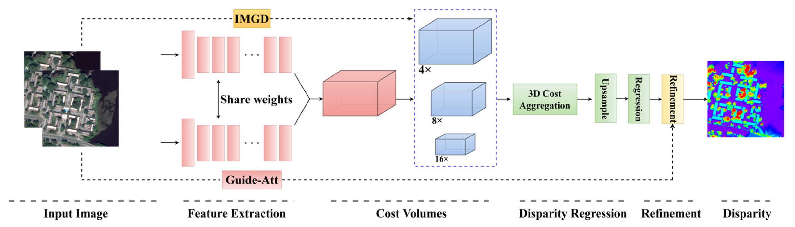
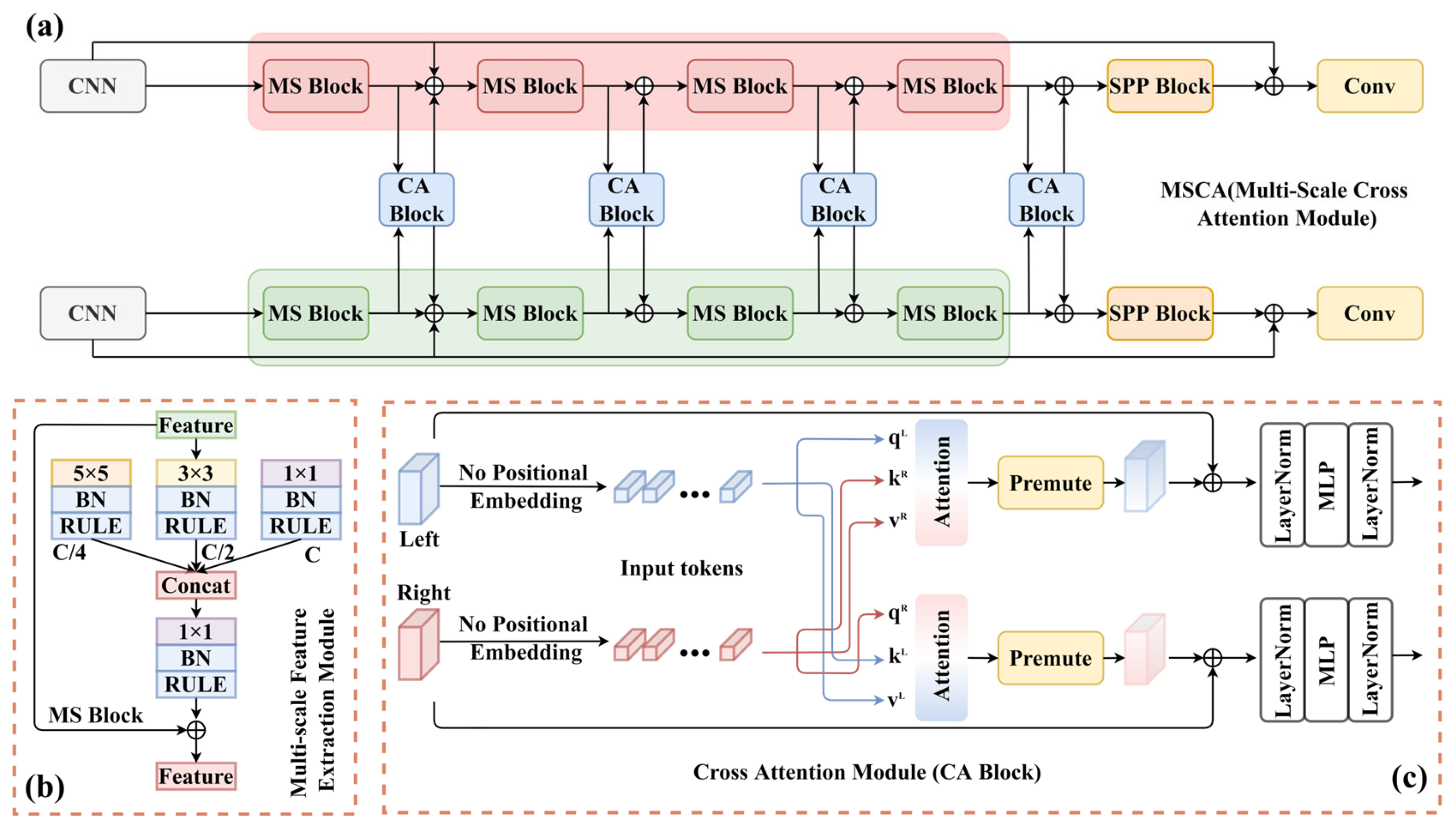
• We propose CAGFNet, an end-to-end deep learning network for disparity estimation. It integrates multi-scale convolution and cross-attention for feature extraction, along with 3D convolution and multi-scale cost volume processing to learn depth relationships across scales, improving precision and robustness;
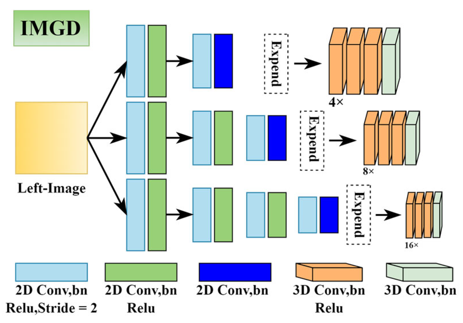
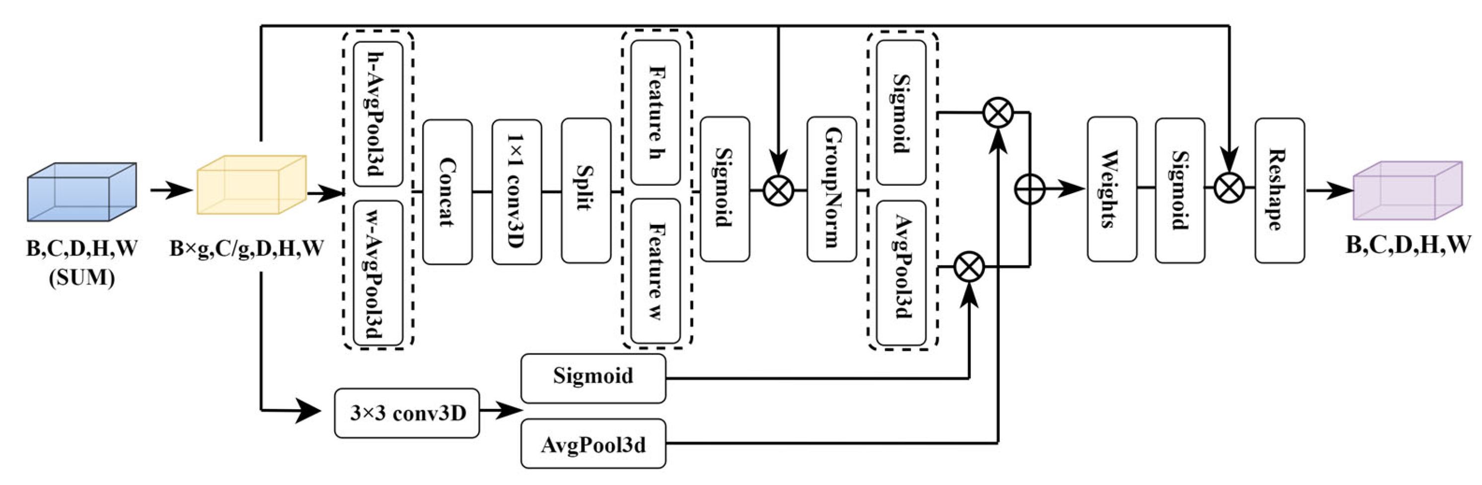
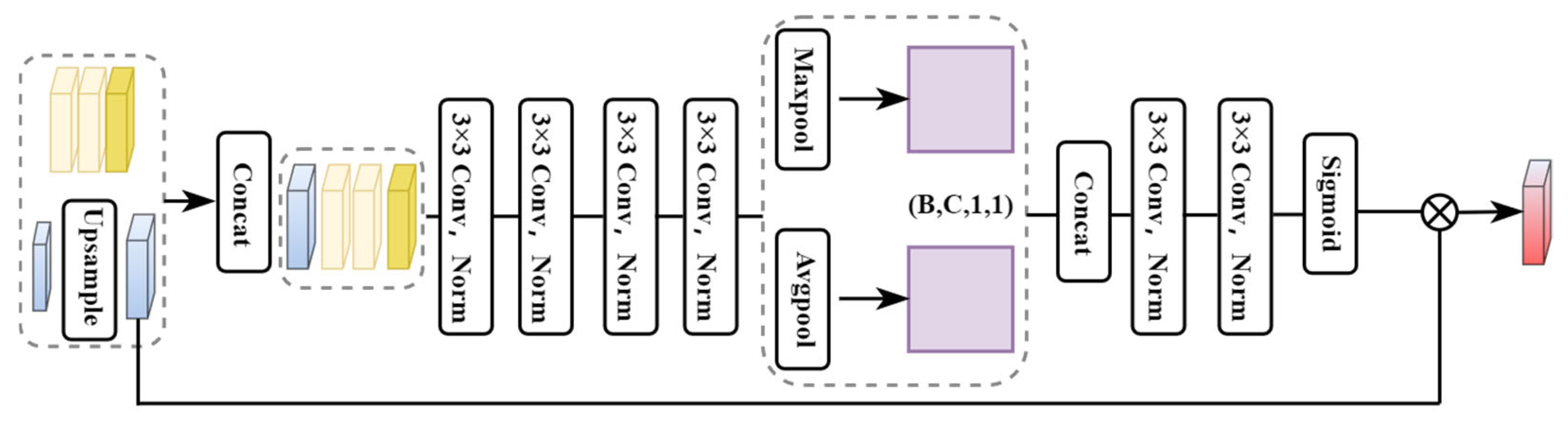
• The IMGD and 3D EMA modules restore and fuse multi-scale features, while the guide attention module refines disparity results, enhancing accuracy in complex scenes;
• Extensive experiments on the US3D and WHU Aerial Stereo datasets validate the functionality of each module and demonstrate the model’s effectiveness and generalization capability.

2. Related Work

End-to-end deep learning methods have revolutionized stereo matching technology by consolidating the traditional multi-step process into a single network, which directly predicts disparity maps from stereo image pairs, significantly improving performance. These methods can be broadly classified into two paradigms: one uses an encoder–decoder structure (e.g., DispNet) to directly regress disparity maps, achieving high accuracy but requiring a large amount of labeled data; the other (e.g., PSMNet) retains a multi-stage architecture while implementing full differentiation, achieving end-to-end optimization through trainable modules such as feature extraction and cost aggregation, striking a better balance between accuracy and data requirements. Both paradigms face the challenge of high labeling costs for remote sensing data, prompting researchers to develop more efficient learning strategies.

MC-CNN [14] introduced deep learning into the field of stereo matching, using CNNs to learn feature matching costs and generating disparity maps via a sliding window, significantly improving matching accuracy, but it did not implement end-to-end learning. DispNet [3] is the first end-to-end model adopting an encoder–decoder structure. CRL [22] improves upon DispNet by using cascaded residual learning to progressively refine disparity estimation. ShapeNet [23] utilizes feature projection and back projection, leveraging 3D geometric properties for measurable 3D reconstruction. GCNet [17] innovatively uses 3D convolutions to optimize the cost volume, effectively addressing occlusion and viewpoint variation issues. iResNet [24] achieves high performance and fast operation through multi-scale features and initial disparity optimization. Stereonet [25] is designed for real-time applications, improving accuracy and edge details through a hierarchical refinement module. PSMNet [26] introduces multi-scale feature extraction and spatial attention mechanisms, significantly enhancing matching accuracy and efficiency. MCUA [27] improves matching accuracy by merging multi-level information to enhance feature representation. GANet [28] enhances the cost volume aggregation accuracy through guided convolutions and non-local optimization modules, demonstrating excellent performance, particularly in large occlusion and repetitive pattern scenarios. GWCNet [29] builds the cost volume using an intra-group correlation module, enhancing the robustness of feature matching. LEAStereo [30] utilizes neural architecture search to automatically optimize the network structure, improving both accuracy and efficiency. STTR [31] incorporates the Transformer architecture, enhancing its robustness and generalization ability. ACVNet [32] optimizes the construction of the cost volume using an attention mechanism to fuse image features in multiple dimensions. CGI-Stereo [33] integrates geometric and contextual information through the CGF module, while AFV constructs an efficient cost volume, balancing real-time performance with high accuracy. ELFNet [34] improves accuracy and robustness in complex scenarios through a local–global feature fusion mechanism. The DeepSim-Nets [35] network, by learning pixel-level matching with contrastive loss, generalizes well to different geometric structures and outperforms hybrid and end-to-end methods. LightStereo [36] optimizes 2D cost aggregation through channel enhancement techniques, improving both computational efficiency and accuracy. Ref. [37] proposed a data-driven neural MRF model that improves stereo matching accuracy and speed by designing latent functions and message passing using neural networks. MC-Stereo [38] innovates a multi-peak search strategy and cascading search range, addressing the multi-peak issue in iterative optimization and improving stereo matching accuracy. Ghost-Stereo [39] is a lightweight stereo matching network based on GhostNet, which enhances performance through the Ghost-CVE and Ghost-CVA modules while reducing computational complexity. MoCha-Stereo [40] optimizes edge matching through the MCCV and REMP modules, improving disparity estimation accuracy. DCVSMNet [41] integrates geometric information through two small cost volumes and a coupling module, offering fast inference and strong generalization ability.

Many innovative works have also emerged in the field of disparity estimation for remote sensing imagery. Ref. [42] proposed an edge-aware bidirectional pyramid network, enhancing accuracy and preserving edge details. Ref. [43] introduced a bidirectional guided attention network, improving 3D semantic detection performance. Ref. [4] proposed a dual-scale matching network, combining features from different scales to improve accuracy in complex scenes. HMSMNet [18] enhances accuracy and efficiency in high-resolution images through multi-level feature fusion and an adaptive multi-scale matching strategy. S²Net [44] improves stereo matching accuracy and robustness by fusing semantic and geometric features through multi-task learning. HF²Net [45] introduces a hybrid feature fusion network that generates high-precision digital surface models, improving 3D reconstruction accuracy. CSStereo [46] combines contrastive learning and feature selection to solve the stereo matching challenges in drone scenarios, achieving superior performance. The novel CNN stereo matching network [47] achieves an inference speed of 92 ms through multi-scale cost volume and negative disparity adaptation. The single-branch network S³Net [48] jointly optimizes semantic segmentation and stereo matching through self-fusion and mutual-fusion modules, improving mIoU to 67.39 and reducing D1-Error to 9.579. SemStereo [49] jointly optimizes semantic segmentation and stereo matching performance through a semantic cascading structure and SSR/LRSC modules. The dual-branch multi-scale stereo matching network [50] integrates disparity attention mechanisms to improve matching accuracy in difficult areas of satellite images, while the model is lightweight.

3. Materials and Methods

Figure 1 illustrates the architecture of CAGFNet, which incorporates three key innovations: (1) multi-scale cross-attention feature extraction, (2) image-guided 3D cost volume fusion, and (3) multi-scale disparity regression and refinement. The network extends PSMNet with improved feature learning and regression modules (details in Section 3).

3.1. Feature Extraction Module

The overall framework is shown in Figure 2a, which we refer to as the MSCA (Multi-Scale Cross-Attention Module). The MSCA module is designed to extract robust features from satellite stereo images by combining two key capabilities: (1) analyzing image content at multiple scales (MS Block) and (2) dynamically focusing on important regions through cross-view attention (CA Block).

First, high-resolution satellite stereo images contain rich detailed information, especially large-scale terrain features, which requires the feature extraction module to process large-scale images while improving efficiency without sacrificing accuracy [51,52]. At the same time, such images often contain vast areas of sparse texture regions (such as water surfaces, deserts, and glaciers), which lack significant matching features and can lead to difficulties in feature extraction [53,54]. To tackle these issues, we adopted a multi-scale feature extraction mechanism similar to RP-Block [55], which captures detailed information at different scales, reduces information loss, and enhances the understanding of sparse texture regions through a convolutional network with multi-layer receptive fields, improving the accuracy and effectiveness of feature extraction. As shown in Figure 2b, multi-scale convolution captures information at different scales using convolution kernels of different sizes (5 × 5, 3 × 3, and 1 × 1). The 5 × 5 convolution kernel covers a larger receptive field and captures large-scale features, such as the overall structure of the image or large areas (e.g., buildings, forests, lakes, etc.). The 3 × 3 convolution kernel is used to capture mid-scale features, balancing computational cost and detail extraction ability, suitable for processing local terrain contours (e.g., roads, rivers, etc.). The 1 × 1 convolution kernel is used to integrate channel information, reduce the number of parameters, and enhance model efficiency while retaining the interrelationships between channels. This parallel multi-scale convolution design ensures that the model can capture both global and local details simultaneously, especially performing well in high-resolution satellite stereo images with complex terrain.

Additionally, satellite stereo images exhibit characteristics such as complex terrain, lighting variations, noise interference, and large-scale disparity variations [56]. These factors accentuate the differences between the left and right views, making it challenging for conventional matching methods to deliver accurate depth information.

To tackle these issues, we designed a Cross-Attention Module (CA Block), which dynamically focuses on key regions in the image and enhances feature selection accuracy by integrating information from both the left and right views. Unlike conventional attention mechanisms that operate within a single view, our CA Block uniquely establishes bidirectional attention relationships between views, enabling more robust feature matching. The core principle of the Cross-Attention Module is that by calculating attention weights between the left and right views, the model can dynamically adjust its focus based on the importance of different regions. Specifically, the CA Block establishes an attention relationship between the left and right views, enabling certain regions in the left image to align with the most relevant parts in the right image and vice versa. In this way, the CA Block effectively addresses matching difficulties caused by differences in perspective, occlusion, or texture variation.

As shown in Figure 2c, the CA Block is not only capable of adapting to global feature extraction but also captures local details, improving matching performance and robustness in complex scenarios. This design of the cross-attention mechanism enables the model to more accurately identify key features in the left and right views, ultimately improving accuracy and demonstrating strong adaptability when handling complex remote sensing images.

The input image is initially processed through a simple CNN architecture (as shown in

Table 1. The CNN framework design in Figure 2a.

Name	Layer Setting	Output Dimension
CNN
Input		H × W × 3
initial_conv	[3 × 3, 132] × 3	$\frac{1}{2}$H × $\frac{1}{2}$W × 32
res_block1	[3 × 3, 132] × 3	$\frac{1}{2}$H × $\frac{1}{2}$W × 32
res_block2	[3 × 3, 164] × 3	$\frac{1}{2}$H × $\frac{1}{2}$W × 64
res_block3	[3 × 3, 128] × 3	$\frac{1}{2}$H × $\frac{1}{2}$W × 128

) before passing through the MS and CA Blocks. By stacking multiple consecutive MS and CA Blocks, the model progressively extracts multi-scale information at different levels. This structure effectively leverages the combination of multi-scale information and the attention mechanism, ensuring the model can capture both global features and critical details with high precision. Additionally, the module incorporates the SPP module to further integrate multi-level feature information, ensuring the effective coordination of both global and local features [26]. The overall design guarantees high accuracy, making it well-suited for handling complex terrain, lighting variations, and noise interference in large-scale scenarios while endowing the model with excellent generalization ability and robustness.

3.2. Cost Volume Construction

The core of cost volume construction involves aligning and computing the difference between the features of the left and right views, generating a tensor that represents disparity information.

We adopted the cost volume construction method used in PSMNet. First, the feature maps of the left and right views are extracted, denoted as $F_L$ and $F_R$, respectively. These feature maps contain spatial information at different levels. For each disparity hypothesis $d$, the feature $F_L$ of the left image, remains unchanged, while the feature $F_R$ of the right image needs to be horizontally shifted (i.e., translated) based on the disparity $d$. The feature of the right image is shifted by $d$ pixels, denoted as $F_R(x+d,y)$, where $\left(x,y\right)$ represents the pixel position. For each disparity hypothesis $d$, the features of the left image and the shifted features of the right image are concatenated along the channel dimension. The formulation for constructing the cost volume is given by Equation (1):

$$C\left(x,y,d\right)=Concat\left(F_L\left(x,y\right),F_R\left(x+d,y\right)\right)$$

(1)

$C\left(x,y,d\right)$ is the cost volume at pixel position $\left(x,y\right)$ and disparity hypothesis $d$. This process is repeated for all pixel positions $\left(x,y\right)$ and for all disparity values $d$, ultimately yielding a 4D cost volume with dimensions H × W × D × 2C, where H and W are the height and width of the image, D is the maximum disparity range, and 2C is the number of channels after concatenating the features of the left and right images. The advantage of this method lies in explicitly constructing the feature alignment relationships for different disparities, allowing the model to effectively perform feature matching in the disparity space, thereby improving the accuracy of depth estimation.

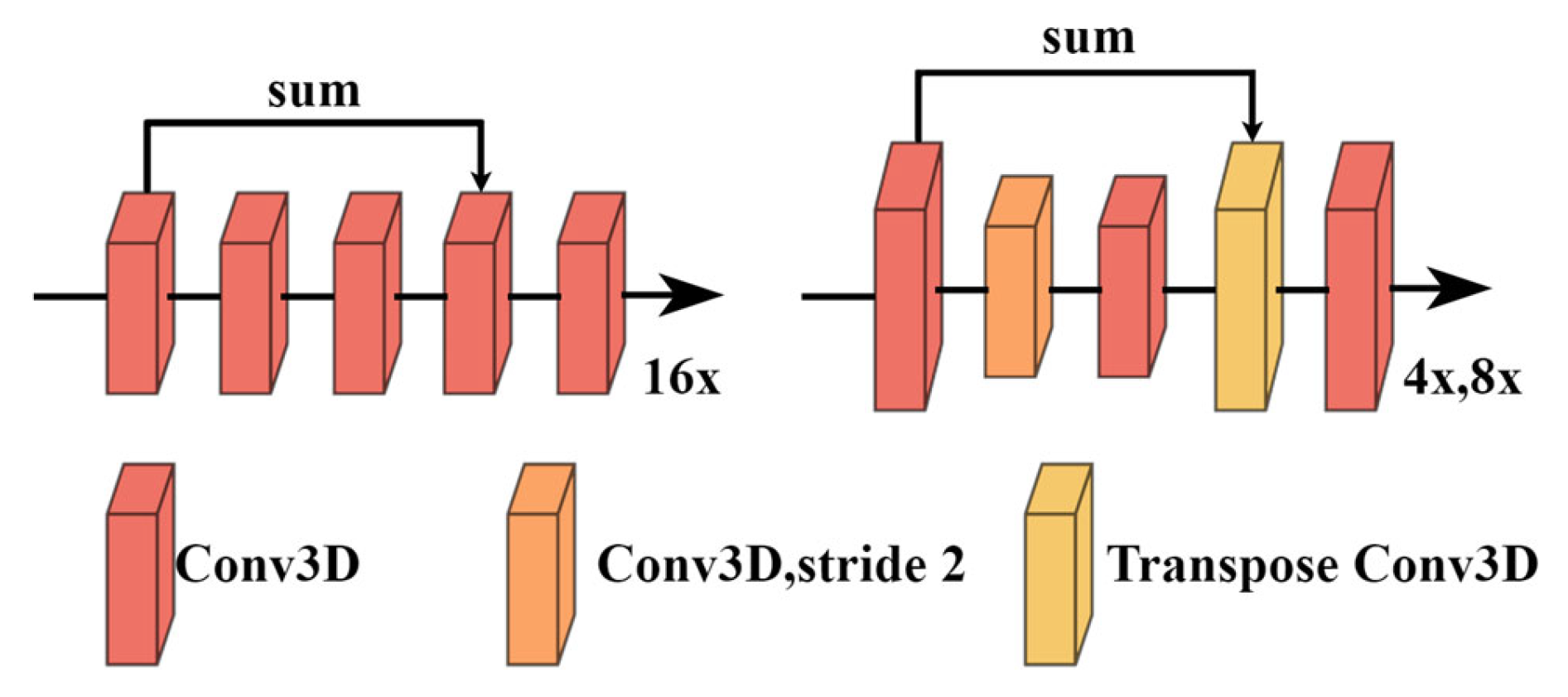
3.3. Three-Dimensional Cost Aggregation

This process integrates and smooths information across disparity layers, which aids in recovering high-quality disparity maps in complex scenes. Inspired by SSPCV-Net [57] and HMSMNet, and taking into account the characteristics of the images, we designed the 3D cost aggregation process, as shown in Figure 3. Unlike SSPCV-Net and HMSMNet, we did not apply pooling to downscale the original extracted features. Instead, we directly applied 3D convolution to the constructed cost volume, generating cost volumes at different scales. This approach avoids the information loss caused by pooling, preserving more details and improving depth inference. Additionally, during this process, we introduced 3D feature information from the original images through the IMGD module, which compensates for the loss of information in deep feature extraction. In terms of feature fusion, we designed a 3D EMA feature fusion module based on EMA [58] to integrate the original image, cost volume, and cost volumes at different scales. The fused cost volume was input into an hourglass module for preliminary cost aggregation and disparity regression, resulting in initial disparity predictions. Finally, the initial disparity results were refined through the feature map guidance module, Guide Attention, to produce the final disparity map.

Image guide (IMGD) module: It employs multi-scale 2D–3D convolutions to extract global-to-local features from the original image, which are then fused with the cost volume to compensate for information loss in deep networks.

As shown in Figure 4, it is implemented using both 2D and 3D convolutions. It employed 4 2D convolutions and 4 3D convolutions to generate a 3D feature module at 1/4 size, focusing on the shallow global information of the original image. Similarly, it employed 6 2D convolutions and 4 3D convolutions to generate a 3D feature module at 1/8 size, focusing on the local information of the original image. Lastly, it employed 8 2D convolutions and 4 3D convolutions to generate a 3D feature module at 1/16 size, focusing on the detailed information of the original image. The feature results of the IMGD module were fused with the corresponding scale of the cost volume using 3DEMA to enhance the feature representation capability of each cost volume and compensating for information loss during the deeper feature processing.

The 3D efficient multi-scale attention (3DEMA) module: It optimizes the feature fusion process across multi-scale cost volumes using an efficient multi-scale attention mechanism.

As shown in Figure 5, it adds the input features to be fused and reshapes them, denoted as $Featur{e}_{group}$, which are then fed into two branch modules, one for the upper and one for the lower part. The upper branch module uses two 3D average pooling layers to separately process the length and width of the input features. The results are concatenated and fed into a 1 × 1 3D convolution layer for feature mixing. The output is then separated and passed through a Sigmoid function, resulting in the output feature, $Featur{e}_{up}$, which can be computed using Equation (2):

$$Featur{e}_{up}=Featur{e}_{group}\ast Featur{e}_h.Sigmoid\left(\right)\ast Featur{e}_w.Sigmoid\left(\right)$$

(2)

$Featur{e}_{up}$ is then separately passed through a Sigmoid function and a 3D average pooling layer.

The lower branch first inputs the $Featur{e}_{group}$ into a 3 × 3 3D convolution layer for feature mixing, producing $Featur{e}_{down}$. This is then passed through a Sigmoid function and a 3D average pooling layer. The result is multiplied by the upper branch output to generate the feature weight vector, weights, which can be computed using Equation (3):

$$\begin{gathered} wights=Featur{e}_{down}.AvgPool3D\left(\right)\ast Featur{e}_{up}.Sigmoid\left(\right) \\ +Featur{e}_{up}.AvgPool3D\left(\right)\ast Featur{e}_{down}.Sigmoid\left(\right) \end{gathered}$$

(3)

Finally, the fused features are output as Feature, which can be computed using Equation (4):

$$Feature=Reshape\left(Featur{e}_{group}\ast weight.Sigmoid\left(\right)\right)$$

(4)

The 3DEMA module batches the input features along the channel dimension and performs feature extraction separately along the height and width. By integrating multi-scale feature extraction and an adaptive feature weighting mechanism, it effectively enhances the recognition ability of object features under complex terrain and lighting conditions. At the same time, by learning the correlation between features, it optimizes feature representation. This enables stronger adaptability and reliability when handling difficult scenarios, such as high disparity, occlusion, and repetitive textures.

We applied different hourglass modules to the cost volumes at different scales, as shown in Figure 6. At the 16× scale, the cost volume undergoes no down-sampling or transposed convolution to avoid excessive down-sampling that could result in the loss of details, thereby preserving high-resolution features. At the 4× and 8× scales, we applied a single down-sampling and transposed convolution to effectively reduce the computational load and capture broader contextual information. This multi-scale processing approach balances computational efficiency with information retention, ensuring the model performs well at all scales. The overall design uses five 3D convolutions, reducing the number of convolution layers to effectively lower computational complexity and memory consumption, thereby improving the model’s operational efficiency. At the same time, the hourglass module, with appropriate processing at different scales, extracts and merges key features across multiple scales, thereby balancing performance and efficiency.

Guide attention module: By fusing image edge features, color information, and the initial disparity map, attention weights are generated via 3D convolution and dual pooling paths to perform pixel-level optimization on the coarse disparity map.

As shown in Figure 7, our feature map guidance module uses the Sobel operator to compute the gradient features of the left and right images. Specifically, we also introduced the Lab color space features of the right image, which, together with the coarse disparity map obtained after disparity regression, formed a 13-channel feature image. This was then input into four 3 × 3 3D convolution modules and normalized. The results were subsequently fed into max pooling and average pooling layers. The results were concatenated and input into two 3 × 3 3D convolutions. After passing through the Sigmoid function, the results were multiplied by the original coarse disparity map to obtain the final refined disparity result.

3.4. Disparity Regression

We used the computation method in Equation (5) to regress disparity:

$$\widehat{d}=\sum _{d=0}^{D_{max}}d\ast p\left(d\right)$$

(5)

The specific procedure is to first restore the regularized cost volume to its original size using trilinear interpolation for up-sampling. Then, the up-sampled cost volume is processed with the Softmax function, converting it into a disparity probability distribution $p\left(d\right)$. The final disparity value is computed by performing a weighted average over the different disparity hypotheses d.

3.5. Loss Function

To optimize disparity estimation accuracy, this model uses the L1 loss function as the regression loss for disparity estimation. The L1 loss function has the advantage of being insensitive to outliers. Compared to the L2 loss function, it is more robust when there are large deviations in the predicted results [59].

Given the predicted disparity map $\widehat{d}(x,y)$ and the ground truth disparity map $d(x,y)$, the $L_1$ loss function is defined as the sum of the absolute differences between the predicted and ground truth, as shown in Equation (6):

$$L_1={\displaystyle \frac{1}{N}}\sum _{\left(x,y\right)}{smooth}_{L_1}\left(d\left(x,y\right)-\widehat{d}\left(x,y\right)\right)$$

(6)

Here,

$${smooth}_{L_1}\left(x\right)=\left\{\begin{array}{l}0.5x^2, if \left|x\right|<1\\ \left|x\right|-0.5,otherwise\end{array}\right.$$

(7)

Here, $N$ represents the total number of pixels in the image, $(x,y)$ denotes the pixel coordinates, $\widehat{d}\left(x,y\right)$ is the predicted disparity at pixel $(x,y)$, and $d(x,y)$ is the corresponding ground truth disparity.

Since the model outputs multiple disparity maps (${Dis}_0,{Dis}_1,{Dis}_2,{Dis}_3$), during the training process, we computed the loss values for all the outputs, as shown in Equation (8):

$$L_{Total}={\lambda }_0\ast {Dis}_0+{\lambda }_1\ast {Dis}_1+{\lambda }_2\ast {Dis}_2+{\lambda }_3\ast {Dis}_3$$

(8)

By supervising disparity maps at different levels, the training process can assign clear stereo semantics to each sequential branch in the network. The result of the previous branch provides guidance for the subsequent branches, which further correct the overall error distribution through the backpropagation of errors, thereby maximizing the accuracy of the final disparity results.

4. Results

In this section, we present the experimental setup and provide a comprehensive evaluation of the performance of CAGFNet, showcasing both the quantitative and visual results.

4.1. Experiment Setting

4.1.1. Datasets

The US3D dataset [60,61] was provided by the IEEE GRSS (Geoscience and Remote Sensing Society) and focuses on 3D reconstruction and stereo matching tasks in urban environments, particularly in the application of high-resolution satellite stereo images. Tracks 2 and 3 of this competition involve stereo matching and 3D modeling tasks. It provides 4292 RGB images, along with corresponding ground truth disparity maps. These images were collected from the WorldView-3 satellite, covering the cities of Jacksonville and Omaha in the United States, with a size of 1024 × 1024 pixels and an image resolution of approximately 0.3 m. All images were preprocessed with RPC-based orthorectification and epipolar rectification to eliminate off-nadir distortions [60,62]. Ground truth disparities were derived from airborne lidar (80 cm ANPS) and projected into rectified coordinates with sub-pixel residual errors (<0.1 px).

The WHU Aerial Stereo dataset [63] was generated from a highly accurate 3D digital surface model (DSM) derived from thousands of real aerial images and refined via manual editing, covering 6.7 × 2.2 km² over Meitan County, China, with 0.1 m ground resolution. The area includes dense high-rise buildings, sparse factories, forested mountains, bare ground, and rivers. The dataset consists of 1776 aerial images (5376 × 5376 pixels) captured at 550 m altitude with 10 cm resolution, organized into 11 flight strips (90% heading overlap and 80% side overlap). All images have fixed orientation angles (0,0,0), ensuring adjacent pairs form epipolar-aligned stereo images. We used its stereo pair subset.

Table 2. Data used in our experiments.

Stereo Pair	Mode	Size	Data Splitting	Usage
Jacksonville	RGB	1024 × 1024	1739/200/200	Training/Validation/Test
Omaha	RGB	1024 × 1024	1753/200/200	Training/Validation/Test
WHU	RGB	768 × 384	240	Test

presents the partitioning of the datasets used in the experiment.

4.1.2. Evaluation Metrics

We used the two metrics proposed by [60] for accuracy evaluation, namely, the average breakpoint error and the error pixel ratio. The formulas for both are as follows:

$$EPE={\displaystyle \frac{1}{N}}\sum _{k\in T}\left|d_k-d_k^{^}\right|$$

(9)

$$D1={\displaystyle \frac{1}{N}}\sum _{k\in T}\left[\left|d_k-d_k^{^}\right|>t\right]$$

(10)

Here, $d_k$ and $d_k^{^}$ represent the ground truth disparity and the estimated disparity, respectively. $N$ and $T$ represent the number of labeled pixels and the set of pixels in the image, respectively, and t is the disparity threshold, typically set to 3. For both error metrics, lower values are preferred.

4.1.3. Training Strategies

We conducted two experiments to assess the performance of the CAGFNet network:

• Train and test separately on the Jacksonville and Omaha subsets to assess the model’s performance;
• Train on one subset and test on the other to evaluate the model’s generalization ability.

4.1.4. Implementation Details

We trained CAGFNet end-to-end using Adam (β₁ = 0.9, β₂ = 0.999) with three key design considerations:

Input size (512 × 256): Balances memory constraints with sufficient spatial context for disparity learning, while maintaining the original image aspect ratio.

Cosine annealing: Gradually reduces the initial 0.001 learning rate over 100 epochs to improve convergence in the final training stages.

Loss weighting (λ₀-₃ = 0.5, 0.5, 0.7, 1): Prioritizes fine-scale disparity refinement (higher weight for deeper outputs).

No data augmentation was applied to preserve the geometric relationships in the original satellite imagery. The 128-pixel maximum disparity accommodates typical urban height variations at the input resolution. The model was trained in a PyTorch 1.11.0 environment on Windows 10 with a batch size of 12. Our computer was equipped with an Intel Xeon Gold 5218R processor (Intel Corporation, Santa Clara, CA, USA) and an NVIDIA A100 Tensor Core GPU (Nvidia Corporation, Santa Clara, CA, USA), along with 128 GB of operating memory.

4.2. Results and Comparisons

DenseMapNet [64], PSMNet [26], StereoNet [25], ACVNet [32], HMSMNet [18], and DCVSMNet [41] were selected for comparison. DenseMapNet is a compact model and acts as the reference baseline for the US3D dataset. PSMNet and StereoNet are classic models in computer vision, representing advanced achievements in deep learning and efficient network architectures, and are widely used in stereo matching tasks. ACVNet and DCVSMNet rank highly in the KITTI benchmark, demonstrating excellent performance in real-world environments. HMSMNet is specifically designed for disparity estimation in remote sensing images, effectively handling complex terrains and uneven lighting conditions. However, these methods have some differences. For a fair comparison, we configured them to be identical to our method, using the same programming language, operating system, and hardware. Below, we evaluate the disparity estimation performance of CAGFNet alongside the comparison models.

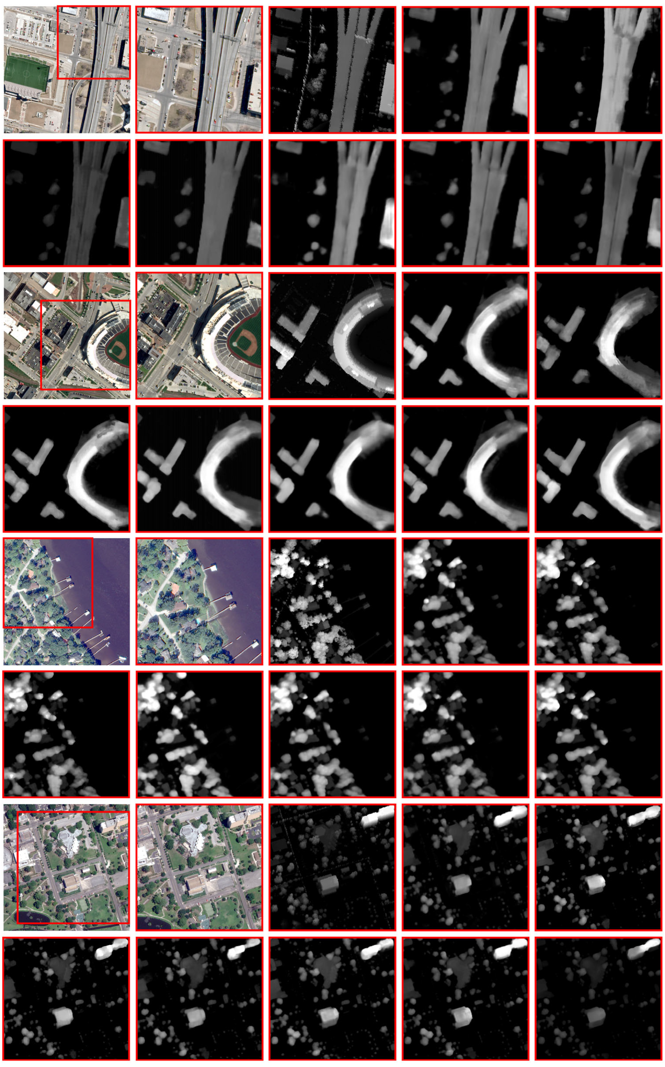
Results on the US3D Dataset

Table 3. Quantitative comparison of different methods on the US3D dataset.

Method	Jacksonville		Omaha
	EPE (Pixel)	D1 (%)	EPE (Pixel)	D1 (%)
DenseMapNet	2.857	33.60	1.306	14.40
StereoNet	1.791	19.01	1.282	14.03
PSMNet	1.711	16.00	1.422	12.92
ACVnet	1.838	17.70	1.632	15.58
HMSMNet	1.529	15.25	1.082	11.53
DCVSMNet	2.034	20.29	1.759	18.59
CAGFNet	1.466	14.71	0.996	10.53

Bold values indicate optimal scores in each metric.

presents the quantitative accuracy comparison for the entire test set of Jacksonville and Omaha. Our proposed CAGFNet yields the best results, significantly surpassing the official baseline. Compared to HMSMNet, on the Jacksonville dataset, EPE and D1 improved by approximately 6% and 5%, respectively, and on the Omaha dataset, EPE and D1 improved by approximately 9% and 10%, respectively.

Figure 8 displays the disparity maps generated by these methods, and our model provides the highest quality disparity results. First, in areas with intricate structures, such as trees and buildings, our model effectively recovers detailed information. Secondly, in regions with disparity discontinuities, our model provides accurate results across all disparity ranges. Additionally, in textureless regions, such as roads, our model produces the smoothest results.

Difficult areas in satellite images make stereo matching challenging. We selected several stereo pairs with typical scenes, including textureless areas, repetitive pattern regions, disparity discontinuities, and occlusion areas, to evaluate these models accurately.

Textureless areas: In textureless regions, pixel intensity variations are minimal, making it difficult to distinguish features, which can lead to poor prediction results. We present the disparity prediction results for these areas in Figure 9. In the overpass area, disparity changes should smoothly decrease or increase. In the first row, we show the disparity prediction results for the overpass region, where our results appear smoother. On the rooftops of houses, water surfaces, and flat grasslands, the disparity results should be consistent and stable. In the second and third rows, we provide such examples, and it is evident that our results are more consistent and stable within the region.

Repeated texture regions: In areas with repeating patterns, the image blocks have similar structures and appearances, causing ambiguous matching. We describe several examples in Figure 10. These images contain similar texture, color, and morphological features. The disparity maps generated by DenseMapNet and StereoNet are almost unusable. In the disparity map predicted by PSMNet, the shapes of some houses are distorted or missing. In the disparity maps predicted by ACVNet, HMSMNet and DCVSMNet, some houses are incorrectly connected to the boundaries of adjacent ones. In contrast, our model successfully distinguishes between house instances and recovers their accurate shapes, thereby reducing ambiguity.

Disparity discontinuity or occlusion areas: Disparity discontinuity may lead to edge-fattening issues [65]. If occlusion exists, matching cannot be performed, and disparity can only be estimated approximately [64]. In Figure 11, we show some examples caused by high features leading to disparity discontinuity and occlusion areas. Compared to other networks, our model effectively mitigates the “edge-thickening” issue at building edges. Except for HMSMNet and CAGFNet, other models gave incorrect disparity predictions in the surrounding ground areas. HMSMNet and DCVSMNet provided incorrect predictions in areas other than the ground, such as the road above a tall building in Figure 11, JAX_264_003_011, where an incorrect high value was predicted. Our model provides more consistent predictions, suggesting that our method better handles the matching of occlusion areas.

From the three image examples above, we qualitatively evaluated the performance of different models.

Table 4. EPE metrics of disparity maps predicted by different models in textureless areas.

	EPE (Pixel)
	DenseMapNet	StereoNet	PSMNet	ACVNet	HMSMNet	DCVSMNet	CAGFNet
JAX_204_004_011	1.606	2.755	1.195	1.194	1.092	1.541	0.975
JAX_156_007_022	2.058	5.463	0.797	0.753	0.71	0.787	0.632
OMA134_003_002	1.369	3.168	1.367	1.319	1.258	1.338	1.095

Bold values indicate optimal scores in each metric.

,

Table 5. D1 metrics of disparity maps predicted by different models in textureless areas.

	D1 (%)
	DenseMapNet	StereoNet	PSMNet	ACVNet	HMSMNet	DCVSMNet	CAGFNet
JAX_204_004_011	18.76	31.92	10.32	10.44	10.23	18.46	10.1
JAX_156_007_022	24.66	46.75	4.47	3.81	3.92	5.38	3.31
OMA134_003_002	15.58	33.49	12.51	11.56	12.5	14.13	11.35

Bold values indicate optimal scores in each metric.

,

Table 6. EPE metrics of disparity maps predicted by different models in repeated texture regions.

	EPE (Pixel)
	DenseMapNet	StereoNet	PSMNet	ACVNet	HMSMNet	DCVSMNet	CAGFNet
JAX_280_023_003	2.709	3.191	1.869	1.753	1.827	2.005	1.711
JAX_427_016_013	2.785	4.211	2.028	2.012	1.907	2.228	1.815
OMA132_003_039	1.155	3.229	1.198	1.074	0.966	1.001	0.875

Bold values indicate optimal scores in each metric.

,

Table 7. D1 metrics of disparity maps predicted by different models in repeated texture regions.

	D1 (%)
	DenseMapNet	StereoNet	PSMNet	ACVNet	HMSMNet	DCVSMNet	CAGFNet
JAX_280_023_003	31.35	35.01	19.23	17.93	18.58	21.79	17.71
JAX_427_016_013	29.22	40.76	20.73	20.58	19.21	23.21	18.85
OMA132_003_039	13.79	31.63	10.45	7.93	8.72	8.78	8.14

Bold values indicate optimal scores in each metric.

,

Table 8. EPE metrics of disparity maps predicted by different models in disparity discontinuity or occlusion areas.

	EPE (Pixel)
	DenseMapNet	StereoNet	PSMNet	ACVNet	HMSMNet	DCVSMNet	CAGFNet
JAX_072_011_006	1.658	2.217	1.296	1.251	1.133	1.261	1.054
JAX_264_003_011	2.608	4.821	1.485	1.126	1.578	1.316	0.996
OMA212_008_030	0.48	2.022	0.753	0.753	0.488	0.632	0.305

Bold values indicate optimal scores in each metric.

and

Table 9. D1 metrics of disparity maps predicted by different models in disparity discontinuity or occlusion areas.

	D1 (%)
	DenseMapNet	StereoNet	PSMNet	ACVNet	HMSMNet	DCVSMNet	CAGFNet
JAX_072_011_006	21.66	24.81	12.13	11.17	10.86	14.03	10.86
JAX_264_003_011	33.02	35.92	12.18	9.55	20	13.94	9.03
OMA212_008_030	5.43	22.24	3.97	3.48	3.18	4.95	2.71

Bold values indicate optimal scores in each metric.

present the quantitative error metrics for each model on each test image, showing that CAGFNet achieves higher accuracy across the board. This is primarily due to the integration of a cross-attention mechanism in the feature extraction network, which computes the attention weights between the left and right views, allowing the model to dynamically adjust its focus based on the importance of different regions. This effectively enhances the model’s matching ability in textureless and repetitive pattern areas, thereby reducing the challenges posed by disparity discontinuities. Secondly, the image-guided module introduces the raw features of the right image, compensating for the information loss in deep feature extraction, particularly enhancing the matching accuracy in disparity discontinuity and occlusion areas, ensuring smoother and more consistent disparity estimation in these regions. The 3D feature fusion module provides more stable feature support by integrating multi-scale features, helping the network effectively handle complex geometric transformations in areas with significant disparity jumps (e.g., disparity discontinuity regions). Finally, the hierarchical disparity prediction module adopts a coarse-to-fine strategy, progressively optimizing disparity estimation from low to high scales, avoiding common errors in matching and disparity jumps in disparity discontinuity and occlusion regions seen in traditional methods. The refinement module combines image gradients and Lab color space information, excelling in restoring local details, particularly in disparity discontinuity and occlusion regions, where it can more accurately recover boundaries and details, ensuring accuracy and structural consistency. The results show that the proposed network performs excellently in handling disparity discontinuities and occlusion issues, significantly improving the matching accuracy and robustness in complex regions.

While our model demonstrates superior performance in repetitive texture regions compared to existing methods like DenseMapNet, StereoNet, PSMNet, ACVNet, HMSMNet, and DCVSMNet—successfully distinguishing house instances and recovering accurate shapes, as shown in Figure 10—certain limitations remain in extreme cases. The primary challenges occur when (1) repeating patterns have intervals smaller than our maximum disparity setting (128 pixels), causing the cross-attention mechanism to occasionally confuse adjacent structures and (2) areas with extremely uniform textures (e.g., large, tiled roofs) lead to a reduced signal-to-noise ratio in the cost volume. Potential solutions being explored include multi-modal fusion with LiDAR data for geometric constraints, the integration of semantic segmentation priors to provide structural awareness, and the development of adaptive attention mechanisms that dynamically adjust receptive fields based on local texture complexity.

5. Discussion

In one section, we conducted generalization and ablation experiments to assess the model generalization ability and the effectiveness of each module.

5.1. Generalization Experiments

In our generalization experiments, we compared the performance of the disparity estimation models.

First, it is worth noting that our model outperforms other models in terms of the EPE metric, achieving the highest accuracy, as shown in

Table 10. Comparison of generalization ability of different models.

	Training Set	Testing Set
		Jacksonville		Omaha
		EPE (Pixel)	D1 (%)	EPE (Pixel)	D1 (%)
DenseMapNet	Jacksonville		29.41	2.512	28.86
	Omaha	2.612
StereoNet	Jacksonville			4.269	35.02
	Omaha	5.041	45.99
PSMNet	Jacksonville			2.118	19.33
	Omaha	2.666	27.48
ACVNet	Jacksonville			2.164	19.87
	Omaha	2.463	25.35
HMSMNet	Jacksonville			1.885	18.44
	Omaha	2.417	26.3
DCVSMNet	Jacksonville			2.064	19.20
	Omaha	2.411	26.4
CAGFNet	Jacksonville			1.87	19.79
	Omaha	2.349	25.77

Bold values indicate optimal scores in each metric.

. This indicates that our model is capable of more accurately estimating disparity at a fine pixel level. The improvement in precision makes it more suitable for practical applications that require detailed handling, particularly tasks that demand high-precision disparity estimation. However, despite our model’s exceptional performance on the EPE metric, the results on the D1 metric are slightly less favorable. The D1 metric reflects the range of disparity estimation errors, i.e., how many pixels of error are considered “acceptable”. Although there is a slight disadvantage on the D1 metric, this gap does not diminish the practical advantages of our model, especially in scenarios where high precision is required. In these cases, our model would excel in handling details and accuracy.

Table 11. Test results of different models on WHU Aerial Stereo dataset.

Method	EPE (Pixel)	D1 (%)	Total Params (MB)	FLOPS (G)
DenseMapNet	38.998	33.44	0.19	7.37
StereoNet	38.943	32.74	0.65	45.99
PSMNet	39.278	33.75	5.22	381.53
ACVnet	37.349	30.28	7.12	436.55
HMSMNet	38.801	33.08	4.51	324.41
DCVSMNet	38.758	32.99	4.29	70.6
CAGFNet	38.573	32.42	5.7	497.71

Bold values indicate optimal scores in each metric.

presents the test results, model parameters, and FLOPS of different models on the WHU Aerial Stereo dataset. Although our model achieved the optimal performance on the Jacksonville and Omaha datasets, it performed worse than ACVNet on the cross-domain tested aerial data. We analyzed that the low-texture regions and dynamic objects in the aerial data led to a decline in the generalization ability of the pretrained weights. The design of the cascaded cost volume based on the attention mechanism in ACVNet may be more adaptable to such scenarios. However, our model outperforms ACVNet in terms of the number of parameters. In the future, we will enhance the generalization ability by fusing the features of aerial data.

In conclusion, our model demonstrates superior performance in high-precision disparity estimation, achieving the lowest EPE on both the Jacksonville and Omaha datasets, which proves its exceptional capability for detail-sensitive applications. While showing slightly higher D1-error than competitors, this trade-off reflects our design emphasis on pixel-level accuracy over error tolerance. The model maintains parameter efficiency compared to ACVNet, despite the latter’s better generalization on aerial data (WHU dataset) due to its attention-based cascaded cost volume design specialized for low-texture regions. Future work will focus on (1) enhancing cross-domain generalization through multi-spectral feature fusion and (2) optimizing the cost volume construction to better handle aerial-specific challenges like dynamic objects while preserving the current advantages in parameter efficiency and precision-critical scenarios.

5.2. Ablation Experiment

We evaluated the contribution of each module in CAGFNet to disparity estimation performance through ablation experiments. The experiments were performed on the US3D dataset, where key modules are progressively removed or replaced to examine the contribution of each module to the overall model performance. The specific experimental design is as follows:

Model I: The feature extraction module of PSMNet is replaced with CAGFNet multi-scale convolution and the cross-attention mechanism (MSCA module) to validate the effectiveness of the feature extraction module.

Model II: The 3D cost aggregation module of PSMNet is replaced with the CAGFNet 3D cost aggregation module to assess the performance improvement provided by the 3D cost aggregation module.

Model III: The 3D feature fusion module (3D EMA module) in CAGFNet is removed to analyze its effect on multi-scale feature fusion.

Model IV: The image-guided module (IMGD module) in CAGFNet is removed to verify its role in restoring original image features.

Model V: The disparity refinement module (refinement module) in CAGFNet is removed to assess its contribution to the final disparity map optimization.

By comparing the performance of the aforementioned variant models, we can quantify the contribution of each module in CAGFNet, thereby validating the rationality and effectiveness of its design. The experimental results indicate that each module significantly contributes to the improvement of disparity estimation accuracy and robustness, further proving the overall design advantage of CAGFNet.

Table 12. Comparison of the results from different models in the ablation experiment.

Model	Jacksonville		Omaha		Total Params (MB)	FLOPS (G)
	EPE (Pixel)	D1 (%)	EPE (Pixel)	D1 (%)
Model Ⅰ (Feature Change)	1.643	14.90	1.270	10.60	5.44	410.53
Model Ⅱ (Cost Change)	1.561	15.70	1.158	10.90	5.48	468.72
Model Ⅲ (Drop 3DEMA)	1.516	15.20	1.063	11.41	5.69	489.11
Model Ⅳ (Drop Image Guide)	1.532	15.32	1.062	11.01	5.22	423.82
Model V(Drop Refinement)	1.581	14.52	1.246	10.71	5.65	489.34
PSMNet	1.711	16.02	1.422	12.91	5.22	381.53
CAGFNet	1.466	14.72	0.996	10.51	5.70	497.71

Bold values indicate optimal scores in each metric.

shows quantitative results of the ablation experiments, and Figure 12 provides the visualization results. The results show that the complete CAGFNet achieves the highest accuracy, while the other five ablation models show a decrease in accuracy compared to the complete CAGFNet, though they still outperform PSMNet.

The accuracy of Model I, after replacing the MSCA module, improved by approximately 7% and 11% in EPE and D1, respectively, on the Jacksonville dataset and by about 15% and 23% on the Omaha dataset. From the visual results, Model I is smoother compared to PSMNet and recovers more details, with additional fine features of the terrain being displayed. We believe that the MSCA module, with its convolution kernels at different scales and the cross-attention mechanism between the left and right images, enables the model to focus on features at various scales and key attributes, thereby improving disparity map recovery.

The accuracy of Model II, after replacing the 3D convolution module, increased by approximately 15% and 3% in EPE and D1 on the Jacksonville dataset and by 26% and 20% on the Omaha dataset. From the visual results, Model II is smoother than PSMNet, but compared to the complete CAGFNet, it lacks some image details, which indirectly highlights the advantages of the MSCA module.

The results of Model III, compared to CAGFNet, show overestimated values in high-disparity regions. We believe that the 3D EMA module, with its batch-wise reorganization and feature extraction at both high and wide scales, demonstrates better adaptability and reliability in handling challenging scenarios such as high disparity, occlusion, and repetitive textures. Compared to CAGFNet, Model IV does not restore image details completely, especially for smaller terrain features. This indicates that by introducing the image guide module, which focuses on shallow information from the original image, the feature representation of each cost volume can be improved, alleviating the loss of information during deep feature extraction. The results of Model V, compared to CAGFNet, show incomplete image detail recovery, with some errors in the recovery of high-disparity regions. Therefore, in designing the refinement module, we intentionally included max pooling and average pooling operations to enhance the model’s ability to capture local details. These pooling operations, combined with image gradient information, further refine the disparity results.

In terms of model parameters, the MSCA module significantly enhances detail recovery capability by introducing multi-scale convolutional kernels and cross-view attention mechanisms while only increasing parameters by 0.22 M and computations by 29 G FLOPs. This leads to reductions of 7% and 15% in the EPE metric on the Jacksonville and Omaha datasets, respectively, and decreases of 11% and 23% in the D1-error metric. Although the 3D cost volume aggregation module incurs higher computational costs (an additional 87.19 G FLOPs), it demonstrates particularly outstanding performance in complex scenarios on the Omaha dataset, achieving a 26% improvement in EPE. Experimental data further confirm the unique advantages of the 3D EMA module in handling high-disparity regions, as well as the critical value of the image guide module in feature preservation. Particularly noteworthy is the refinement module, which innovatively combines max pooling and average pooling operations to reduce local detail recovery errors by 13–17%. Overall, through synergistic optimization of these modules, CAGFNet achieves reductions of 24% and 42% in EPE metrics on the Jacksonville and Omaha datasets, respectively, at the cost of only a 0.48 M parameter increase, demonstrating an excellent performance–computation efficiency balance. That said, we acknowledge that the current computational scale of 5.70 M parameters and 497.71 G FLOPs does increase computational overheads to some extent, which will be an important direction for future optimization work.

6. Conclusions

This paper presents a novel end-to-end deep learning model, CAGFNet, for the disparity estimation of high-resolution satellite stereo images. The network incorporates a cross-attention mechanism to extract key features and employs a hierarchical learning strategy to refine the disparity estimation layer by layer. Additionally, an image-guided module and a 3D feature fusion module were designed to integrate prior information from the original optical images, effectively compensating for information loss during deep feature extraction. Finally, an image guide attention module was used to regress high-quality, full-resolution disparity maps, ensuring the precise preservation of local structures. A comprehensive comparison with several classic stereo matching networks demonstrates that the proposed network excels in high-resolution remote sensing image disparity estimation tasks, particularly in handling disparity discontinuities and occlusion areas. The EPE and D1 on the Jacksonville subset of the US3D dataset are 1.466 and 14.71%, respectively, while on the Omaha subset, the EPE and D1 are 0.996 and 10.53%, respectively. Moreover, comprehensive ablation experiments validate the effectiveness of each module in the proposed design.

The method shows potential for practical applications in defense, urban planning, and disaster monitoring, where accurate disparity estimation is required. Future work will focus on (1) optimizing model efficiency through parameter reduction techniques, (2) extending validation to additional satellite sensors like GaoFen-7, and (3) investigating fusion with auxiliary data sources such as LiDAR for improved accuracy in complex terrain. The code will be made available to support further research in this field.

References

1. Laga, H.; Jospin, L.V.; Boussaid, F.; Bennamoun, M. A survey on deep learning techniques for stereo-based depth estimation. IEEE Trans. Pattern Anal. Mach. Intell. 2020, 44, 1738–1764. [Google Scholar] [CrossRef] [PubMed]
2. Tulyakov, S.; Ivanov, A.; Fleuret, F. Practical deep stereo (pds): Toward applications-friendly deep stereo matching. Adv. Neural Inf. Process. Syst. 2018, 31, 5875–5885. [Google Scholar]
3. Mayer, N.; Ilg, E.; Hausser, P.; Fischer, P.; Cremers, D.; Dosovitskiy, A.; Brox, T. A large dataset to train convolutional networks for disparity, optical flow, and scene flow estimation. In Proceedings of the IEEE Conference on Computer Vision and Pattern Recognition, Las Vegas, NV, USA, 27–30 June 2016; pp. 4040–4048. [Google Scholar]
4. He, S.; Zhou, R.; Li, S.; Jiang, S.; Jiang, W. Disparity estimation of high-resolution remote sensing images with dual-scale matching network. Remote Sens. 2021, 13, 5050. [Google Scholar] [CrossRef]
5. Horn, B.K.; Schunck, B.G. Determining optical flow. Artif. Intell. 1981, 17, 185–203. [Google Scholar] [CrossRef]
6. Kolmogorov, V.; Zabih, R. Computing visual correspondence with occlusions using graph cuts. In Proceedings of the Eighth IEEE International Conference on Computer Vision, Vancouver, BC, Canada, 7–14 July 2001; pp. 508–515. [Google Scholar]
7. Sun, J.; Zheng, N.-N.; Shum, H.-Y. Stereo matching using belief propagation. IEEE Trans. Pattern Anal. Mach. Intell. 2003, 25, 787–800. [Google Scholar]
8. Veksler, O. Stereo correspondence by dynamic programming on a tree. In Proceedings of the 2005 IEEE Computer Society Conference on Computer Vision and Pattern Recognition, San Diego, CA, USA, 20–25 June 2005; pp. 384–390. [Google Scholar]
9. Hirschmuller, H. Accurate and efficient stereo processing by semi-global matching and mutual information. In Proceedings of the 2005 IEEE Computer Society Conference on Computer Vision and Pattern Recognition, San Diego, CA, USA, 20–25 June 2005; pp. 807–814. [Google Scholar]
10. Redmon, J.; Divvala, S.; Girshick, R.; Farhadi, A. You only look once: Unified, real-time object detection. In Proceedings of the IEEE Conference on Computer Vision and Pattern Recognition, Las Vegas, NV, USA, 27–30 June 2016; pp. 779–788. [Google Scholar]
11. Chen, L.-C.; Papandreou, G.; Kokkinos, I.; Murphy, K.; Yuille, A.L. Deeplab: Semantic image segmentation with deep convolutional nets, atrous convolution, and fully connected crfs. IEEE Trans. Pattern Anal. Mach. Intell. 2017, 40, 834–848. [Google Scholar] [CrossRef]
12. Eigen, D.; Fergus, R. Predicting depth, surface normals and semantic labels with a common multi-scale convolutional architecture. In Proceedings of the IEEE International Conference on Computer Vision, Santiago, Chile, 7–13 December 2015; pp. 2650–2658. [Google Scholar]
13. Luo, W.; Schwing, A.G.; Urtasun, R. Efficient deep learning for stereo matching. In Proceedings of the IEEE Conference on Computer Vision and Pattern Recognition, Las Vegas, NV, USA, 27–30 June 2016; pp. 5695–5703. [Google Scholar]
14. Žbontar, J.; LeCun, Y. Stereo matching by training a convolutional neural network to compare image patches. J. Mach. Learn. Res. 2016, 17, 1–32. [Google Scholar]
15. Yang, G.; Manela, J.; Happold, M.; Ramanan, D. Hierarchical deep stereo matching on high-resolution images. In Proceedings of the IEEE/CVF Conference on Computer Vision and Pattern Recognition, Long Beach, CA, USA, 15–20 June 2019; pp. 5515–5524. [Google Scholar]
16. Cheng, X.; Wang, P.; Yang, R. Learning depth with convolutional spatial propagation network. IEEE Trans. Pattern Anal. Mach. Intell. 2019, 42, 2361–2379. [Google Scholar] [CrossRef]
17. Kendall, A.; Martirosyan, H.; Dasgupta, S.; Henry, P.; Kennedy, R.; Bachrach, A.; Bry, A. End-to-end learning of geometry and context for deep stereo regression. In Proceedings of the IEEE International Conference on Computer Vision, Venice, Italy, 22–29 October 2017; pp. 66–75. [Google Scholar]
18. He, S.; Li, S.; Jiang, S.; Jiang, W. HMSM-Net: Hierarchical multi-scale matching network for disparity estimation of high-resolution satellite stereo images. ISPRS J. Photogramm. Remote Sens. 2022, 188, 314–330. [Google Scholar] [CrossRef]
19. He, X.; Jiang, S.; He, S.; Li, Q.; Jiang, W.; Wang, L. Deep learning-based stereo matching for high-resolution satellite images: A comparative evaluation. Int. Arch. Photogramm. Remote Sens. Spat. Inf. Sci. 2023, 48, 1635–1642. [Google Scholar] [CrossRef]
20. Li, S.; He, S.; Jiang, S.; Jiang, W.; Zhang, L. WHU-stereo: A challenging benchmark for stereo matching of high-resolution satellite images. IEEE Trans. Geosci. Remote Sens. 2023, 61, 1–14. [Google Scholar] [CrossRef]
21. Hirschmuller, H. Stereo processing by semiglobal matching and mutual information. IEEE Trans. Pattern Anal. Mach. Intell. 2007, 30, 328–341. [Google Scholar] [CrossRef] [PubMed]
22. Pang, J.; Sun, W.; Ren, J.S.; Yang, C.; Yan, Q. Cascade residual learning: A two-stage convolutional neural network for stereo matching. In Proceedings of the IEEE International Conference on Computer Vision Workshops, Venice, Italy, 22–29 October 2017; pp. 887–895. [Google Scholar]
23. Kar, A.; Häne, C.; Malik, J. Learning a multi-view stereo machine. Adv. Neural Inf. Process. Syst. 2017, 30, 365–376. [Google Scholar]
24. Liang, Z.; Feng, Y.; Guo, Y.; Liu, H.; Chen, W.; Qiao, L.; Zhou, L.; Zhang, J. Learning for disparity estimation through feature constancy. In Proceedings of the IEEE Conference on Computer Vision and Pattern Recognition, Salt Lake City, UT, USA, 18–23 June 2018; pp. 2811–2820. [Google Scholar]
25. Khamis, S.; Fanello, S.; Rhemann, C.; Kowdle, A.; Valentin, J.; Izadi, S. Stereonet: Guided hierarchical refinement for real-time edge-aware depth prediction. In Proceedings of the European Conference on Computer Vision, Munich, Germany, 8–14 September 2018; pp. 573–590. [Google Scholar]
26. Chang, J.-R.; Chen, Y.-S. Pyramid stereo matching network. In Proceedings of the IEEE Conference on Computer Vision and Pattern Recognition, Salt Lake City, UT, USA, 18–23 June 2018; pp. 5410–5418. [Google Scholar]
27. Nie, G.-Y.; Cheng, M.-M.; Liu, Y.; Liang, Z.; Fan, D.-P.; Liu, Y.; Wang, Y. Multi-level context ultra-aggregation for stereo matching. In Proceedings of the IEEE/CVF Conference on Computer Vision and Pattern Recognition, Long Beach, CA, USA, 15–20 June 2019; pp. 3283–3291. [Google Scholar]
28. Zhang, F.; Prisacariu, V.; Yang, R.; Torr, P.H. Ga-net: Guided aggregation net for end-to-end stereo matching. In Proceedings of the IEEE/CVF Conference on Computer Vision and Pattern Recognition, Long Beach, CA, USA, 15–20 June 2019; pp. 185–194. [Google Scholar]
29. Guo, X.; Yang, K.; Yang, W.; Wang, X.; Li, H. Group-wise correlation stereo network. In Proceedings of the IEEE/CVF Conference on Computer Vision and Pattern Recognition, Long Beach, CA, USA, 15–20 June 2019; pp. 3273–3282. [Google Scholar]
30. Cheng, X.; Zhong, Y.; Harandi, M.; Dai, Y.; Chang, X.; Li, H.; Drummond, T.; Ge, Z. Hierarchical neural architecture search for deep stereo matching. Adv. Neural Inf. Process. Syst. 2020, 33, 22158–22169. [Google Scholar]
31. Li, Z.; Liu, X.; Drenkow, N.; Ding, A.; Creighton, F.X.; Taylor, R.H.; Unberath, M. Revisiting stereo depth estimation from a sequence-to-sequence perspective with transformers. In Proceedings of the IEEE/CVF International Conference on Computer Vision, Montreal, QC, Canada, 10–17 October 2021; pp. 6197–6206. [Google Scholar]
32. Xu, G.; Cheng, J.; Guo, P.; Yang, X. Attention concatenation volume for accurate and efficient stereo matching. In Proceedings of the IEEE/CVF Conference on Computer Vision and Pattern Recognition, New Orleans, LA, USA, 18–24 June 2022; pp. 12981–12990. [Google Scholar]
33. Xu, G.; Zhou, H.; Yang, X. Cgi-stereo: Accurate and real-time stereo matching via context and geometry interaction. arXiv 2023, arXiv:2301.02789. [Google Scholar]
34. Lou, J.; Liu, W.; Chen, Z.; Liu, F.; Cheng, J. Elfnet: Evidential local-global fusion for stereo matching. In Proceedings of the IEEE/CVF International Conference on Computer Vision, Paris, France, 1–6 October 2023; pp. 17784–17793. [Google Scholar]
35. Chebbi, M.A.; Rupnik, E.; Pierrot-Deseilligny, M.; Lopes, P. Deepsim-nets: Deep similarity networks for stereo image matching. In Proceedings of the IEEE/CVF Conference on Computer Vision and Pattern Recognition, Vancouver, BC, Canada, 17–24 June 2023; pp. 2097–2105. [Google Scholar]
36. Guo, X.; Zhang, C.; Nie, D.; Zheng, W.; Zhang, Y.; Chen, L. Lightstereo: Channel boost is all your need for efficient 2d cost aggregation. arXiv 2024, arXiv:2406.19833. [Google Scholar]
37. Guan, T.; Wang, C.; Liu, Y.-H. Neural markov random field for stereo matching. In Proceedings of the IEEE/CVF Conference on Computer Vision and Pattern Recognition, Seattle, WA, USA, 16–22 June 2024; pp. 5459–5469. [Google Scholar]
38. Feng, M.; Cheng, J.; Jia, H.; Liu, L.; Xu, G.; Yang, X. Mc-stereo: Multi-peak lookup and cascade search range for stereo matching. In Proceedings of the 2024 International Conference on 3D Vision (3DV), Davos, Switzerland, 18–21 March 2024; pp. 344–353. [Google Scholar]
39. Jiang, X.; Bian, X.; Guo, C. Ghost-Stereo: GhostNet-based Cost Volume Enhancement and Aggregation for Stereo Matching Networks. arXiv 2024, arXiv:2405.14520. [Google Scholar]
40. Chen, Z.; Long, W.; Yao, H.; Zhang, Y.; Wang, B.; Qin, Y.; Wu, J. Mocha-stereo: Motif channel attention network for stereo matching. In Proceedings of the IEEE/CVF Conference on Computer Vision and Pattern Recognition, Seattle, WA, USA, 16–22 June 2024; pp. 27768–27777. [Google Scholar]
41. Tahmasebi, M.; Huq, S.; Meehan, K.; McAfee, M. DCVSMNet: Double cost volume stereo matching network. Neurocomputing 2025, 618, 129002. [Google Scholar] [CrossRef]
42. Tao, R.; Xiang, Y.; You, H. An edge-sense bidirectional pyramid network for stereo matching of vhr remote sensing images. Remote Sens. 2020, 12, 4025. [Google Scholar] [CrossRef]
43. Rao, Z.; He, M.; Zhu, Z.; Dai, Y.; He, R. Bidirectional guided attention network for 3-D semantic detection of remote sensing images. IEEE Trans. Geosci. Remote Sens. 2020, 59, 6138–6153. [Google Scholar] [CrossRef]
44. Liao, P.; Zhang, X.; Chen, G.; Wang, T.; Li, X.; Yang, H.; Zhou, W.; He, C.; Wang, Q. S2Net: A Multi-task Learning Network for Semantic Stereo of Satellite Image Pairs. IEEE Trans. Geosci. Remote Sens. 2023, 62, 5601313. [Google Scholar] [CrossRef]
45. Zheng, Z.; Wan, Y.; Zhang, Y.; Hu, Z.; Wei, D.; Yao, Y.; Zhu, C.; Yang, K.; Xiao, R. Digital surface model generation from high-resolution satellite stereos based on hybrid feature fusion network. Photogramm. Rec. 2024, 39, 36–66. [Google Scholar] [CrossRef]
46. Cao, X.; Zhang, X.; Yu, A.; Yu, W.; Bu, S. CSStereo: A UAV scenarios stereo matching network enhanced with contrastive learning and feature selection. Int. J. Appl. Earth Obs. Geoinf. 2024, 134, 104189. [Google Scholar] [CrossRef]
47. Wei, K.; Huang, X.; Li, H. Stereo matching method for remote sensing images based on attention and scale fusion. Remote Sens. 2024, 16, 387. [Google Scholar] [CrossRef]
48. Yang, Q.; Chen, G.; Tan, X.; Wang, T.; Wang, J.; Zhang, X. S3Net: Innovating Stereo Matching and Semantic Segmentation with a Single-Branch Semantic Stereo Network in Satellite Epipolar Imagery. In Proceedings of the IGARSS 2024—2024 IEEE International Geoscience and Remote Sensing Symposium, Athens, Greece, 7–12 July 2024; pp. 8737–8740. [Google Scholar]
49. Chen, C.; Zhao, L.; He, Y.; Long, Y.; Chen, K.; Wang, Z.; Hu, Y.; Sun, X. SemStereo: Semantic-Constrained Stereo Matching Network for Remote Sensing. arXiv 2024, arXiv:2412.12685. [Google Scholar] [CrossRef]
50. Xu, Z.; Jiang, Y.; Wang, J.; Wang, Y. A Dual Branch Multi-scale Stereo Matching Network for High-resolution Satellite Remote Sensing Images. IEEE J. Sel. Top. Appl. Earth Obs. Remote Sens. 2024, 18, 949–964. [Google Scholar] [CrossRef]
51. Yin, A.; Ren, C.; Yan, Z.; Xue, X.; Yue, W.; Wei, Z.; Liang, J.; Zhang, X.; Lin, X. HRU-Net: High-Resolution Remote Sensing Image Road Extraction Based on Multi-Scale Fusion. Appl. Sci. 2023, 13, 8237. [Google Scholar] [CrossRef]
52. Zhou, X.; Wei, X. Feature Aggregation Network for Building Extraction from High-Resolution Remote Sensing Images. In Proceedings of the Pacific Rim International Conference on Artificial Intelligence, Jakarta, Indonesia, 15–19 November 2023; pp. 105–116. [Google Scholar]
53. Chu, X.; Yao, X.; Duan, H.; Chen, C.; Li, J.; Pang, W. Glacier extraction based on high-spatial-resolution remote-sensing images using a deep-learning approach with attention mechanism. Cryosphere 2022, 16, 4273–4289. [Google Scholar] [CrossRef]
54. Wu, P.; Fu, J.; Yi, X.; Wang, G.; Mo, L.; Maponde, B.T.; Liang, H.; Tao, C.; Ge, W.; Jiang, T. Research on water extraction from high resolution remote sensing images based on deep learning. Front. Remote Sens. 2023, 4, 1283615. [Google Scholar] [CrossRef]
55. Li, Z.; He, W.; Li, J.; Lu, F.; Zhang, H. Learning without Exact Guidance: Updating Large-scale High-resolution Land Cover Maps from Low-resolution Historical Labels. In Proceedings of the IEEE/CVF Conference on Computer Vision and Pattern Recognition, Seattle, WA, USA, 16–22 June 2024; pp. 27717–27727. [Google Scholar]
56. Wang, Y.; Dong, M.; Ye, W.; Liu, D.; Gan, G. A contrastive learning-based iterative network for remote sensing image super-resolution. Multimed. Tools Appl. 2024, 83, 8331–8357. [Google Scholar] [CrossRef]
57. Wu, Z.; Wu, X.; Zhang, X.; Wang, S.; Ju, L. Semantic stereo matching with pyramid cost volumes. In Proceedings of the IEEE/CVF International Conference on Computer Vision, Seoul, Republic of Korea, 27 October–2 November 2019; pp. 7484–7493. [Google Scholar]
58. Ouyang, D.; He, S.; Zhang, G.; Luo, M.; Guo, H.; Zhan, J.; Huang, Z. Efficient multi-scale attention module with cross-spatial learning. In Proceedings of the ICASSP 2023—2023 IEEE International Conference on Acoustics, Speech and Signal Processing, Rhodes Island, Greece, 4–10 June 2023; pp. 1–5. [Google Scholar]
59. Girshick, R. Fast r-cnn. In Proceedings of the IEEE International Conference on Computer Vision, Santiago, Chile, 7–13 December 2015; pp. 1440–1448. [Google Scholar]
60. Bosch, M.; Foster, K.; Christie, G.; Wang, S.; Hager, G.D.; Brown, M. Semantic stereo for incidental satellite images. In Proceedings of the 2019 IEEE Winter Conference on Applications of Computer Vision, Waikoloa, HI, USA, 7–11 January 2019; pp. 1524–1532. [Google Scholar]
61. Le Saux, B.; Yokoya, N.; Hansch, R.; Brown, M.; Hager, G. 2019 data fusion contest [technical committees]. IEEE Geosci. Remote Sens. Mag. 2019, 7, 103–105. [Google Scholar] [CrossRef]
62. De Franchis, C.; Meinhardt-Llopis, E.; Michel, J.; Morel, J.-M.; Facciolo, G. On stereo-rectification of pushbroom images. In Proceedings of the 2014 IEEE International Conference on Image Processing, Paris, France, 27–30 October 2014; pp. 5447–5451. [Google Scholar]
63. Liu, J.; Ji, S. A novel recurrent encoder-decoder structure for large-scale multi-view stereo reconstruction from an open aerial dataset. In Proceedings of the IEEE/CVF Conference on Computer Vision and Pattern Recognition, Seattle, WA, USA, 13–19 June 2020; pp. 6050–6059. [Google Scholar]
64. Atienza, R. Fast disparity estimation using dense networks. In Proceedings of the 2018 IEEE International Conference on Robotics and Automation, Brisbane, QLD, Australia, 21–25 May 2018; pp. 3207–3212. [Google Scholar]
65. Xu, H.; Zhang, J. Aanet: Adaptive aggregation network for efficient stereo matching. In Proceedings of the IEEE/CVF Conference on Computer Vision and Pattern Recognition, Seattle, WA, USA, 13–19 June 2020; pp. 1959–1968. [Google Scholar]
Figure 1. CAGFNet module.
Remotesensing 17 01572 g001
Figure 2. MSCA module, (a) Multi-Scale Cross Attention Module; (b) Multi-scale Feature Extraction Module; (c) Cross Attention Module.
Remotesensing 17 01572 g002
Figure 3. The 3D cost aggregation module.
Remotesensing 17 01572 g003
Figure 4. Image guide module.
Remotesensing 17 01572 g004
Figure 5. The 3D efficient multi-scale attention module.
Remotesensing 17 01572 g005
Figure 6. Hourglass module.
Remotesensing 17 01572 g006
Figure 7. Image guide attention module.
Remotesensing 17 01572 g007
Figure 8. The disparity maps. From top to bottom: right image, ground truth, DenseMapNet, StereoNet, PSMNet, ACVNet, HMSMNet, DCVSMNet, and CAGFNet. Image IDs are JAX_018_002_012, JAX_118_004_009, JAX_168_023_012, OMA_287_005_001, and OMA_315_040_008.
Remotesensing 17 01572 g008
Figure 9. The disparity maps in textureless areas. From left to right: right image, ground truth, DenseMapNet, StereoNet, PSMNet, ACVNet, HMSMNet, DCVSMNet, and CAGFNet. Image IDs are JAX_204_004_011, JAX_156_007_022, and OMA134_003_002. The red box indicates the locally magnified area, while the yellow box highlights the key disparity range of the target region.
Remotesensing 17 01572 g009
Figure 10. The disparity maps in repeated pattern regions. From left to right: right image, ground truth, DenseMapNet, StereoNet, PSMNet, ACVNet, HMSMNet, DCVSMNet, and CAGFNet. Image IDs are JAX_280_023_003, JAX_427_016_013, and OMA132_003_039. The red box indicates the locally magnified area, while the yellow box highlights the key disparity range of the target region.
Remotesensing 17 01572 g010
Figure 11. The disparity maps in disparity discontinuity or occlusion areas. From left to right: right image, ground truth, DenseMapNet, StereoNet, PSMNet, ACVNet, HMSMNet, DCVSMNet, and CAGFNet. Image IDs are JAX_072_011_006, JAX_264_003_011, and OMA212_008_030. The red box indicates the locally magnified area, while the yellow box highlights the key disparity range of the target region.
Remotesensing 17 01572 g011
Figure 12. The disparity maps. From left to right: right view, locally magnified right view, locally magnified ground truth disparity map, locally magnified CAGFNet results, locally magnified PSMNet results, locally magnified Model I results, locally magnified Model II results, locally magnified Model III results, locally magnified Model IV results, and locally magnified Model V results. Image IDs are OMA_247_023_025, OMA_248_002_028, JAX_269_004_002, and JAX_122_016_013. The red box indicates the locally magnified area.
Remotesensing 17 01572 g012