Accelerated and Interpretable Flood Susceptibility Mapping Through Explainable Deep Learning with Hydrological Prior Knowledge

Abstract

Flooding is one of the most devastating natural disasters worldwide, with increasing frequency due to climate change. Traditional hydrological models require extensive data and computational resources, while machine learning (ML) models struggle to capture spatial dependencies. To address this, we propose a modified U-Net architecture that integrates prior hydrological knowledge of permanent water bodies to improve flood susceptibility mapping in Northumberland County, UK. By embedding domain-specific insights, our model achieves a higher area under the curve (AUC) (0.97) compared to the standard U-Net (0.93), while also reducing training time by converging three times faster. Additionally, we integrate a Grad-CAM module to provide visualisations explaining the areas of attention from the model, enabling interpretation of its decision-making, thus reducing barriers to its practical implementation.

1. Introduction

Flooding is among the most frequent and destructive natural disasters worldwide, with severe economic and environmental consequences [1]. The increasing intensity of flood events due to climate change has exacerbated the risks, particularly in vulnerable regions with inadequate flood mitigation infrastructure [2]. The ability to predict and map flood susceptibility accurately is crucial for implementing timely disaster mitigation strategies, allowing governments and stakeholders to take pre-emptive action. As a result, there is a growing demand for flood susceptibility models that are not only accurate and scalable but also interpretable for decision-makers and stakeholders.

Physically based hydrological models simulate flood dynamics by integrating terrain properties, precipitation, infiltration, and hydrological flow patterns. Well-established frameworks such as HEC-RAS, LISFLOOD, and MIKE FLOOD exemplify this approach, providing detailed inundation predictions via coupled 1D–2D simulations of rivers and floodplains [3]. These physics-driven models can be generalised to large, data-sparse regions (e.g., rural basins with few gauges) by leveraging remote sensing inputs and robust process representations [4]. Recent advancements in numerical solvers, high-performance computing, and global datasets have dramatically expanded the scale and fidelity of physically based models, enabling continental and even global flood hazard mapping [5].

However, these models require extensive calibration with high-resolution precipitation and streamflow data, which is often unavailable in many regions [6]. Additionally, the computational demands of simulating large-scale flood events make these models challenging to deploy for real-time applications [7]. As a result, alternative data-driven approaches have gained traction, leveraging machine learning (ML) and remote sensing techniques to predict flood susceptibility with reduced reliance on ground-based hydrological measurements [8].

ML models such as artificial neural networks (ANNs) [9,10], support vector machines (SVMs) [8,11,12], random forest (RF) [13,14], and ensemble methods such as XGBoost and LightGBM [15] have demonstrated strong performance and improved flexibility over traditional hydrological models. These models operate on handcrafted environmental features such as elevation, slope, and land cover, and have achieved competitive performance in many flood susceptibility studies. For example, Ren et al. [16] found that RF outperformed SVM and ANN in ensemble configurations, achieving area under the curve (AUC) scores of about 0.87, 0.82, and 0.83, respectively.

While these models offer advantages like computational efficiency and feature interpretability (e.g., feature importance in RF), they treat geographic locations independently, ignoring the spatial continuity of flooding. They also rely heavily on the quality of feature engineering and often require preprocessing techniques such as spatial interpolation to account for spatial dependencies [17]. As a result, traditional ML models may produce fragmented susceptibility maps and exhibit limited generalisation to unseen regions with different physical characteristics.

To address the limitations of traditional ML methods, deep learning models, particularly convolutional neural networks (CNNs), have been increasingly used for flood susceptibility mapping. CNNs excel at processing spatially structured data, such as satellite imagery, digital elevation models (DEMs), and land cover data, by capturing hierarchical feature dependencies [8,18,19]. Among CNN architectures, U-Net has emerged as a leading approach for pixel-wise classification, making it well-suited for generating high-resolution flood susceptibility maps. The encoder–decoder structure of U-Net allows it to learn spatial flood patterns effectively while preserving fine-grained topographic details [20,21].

However, early CNN architectures lacked the ability to produce fine-grained, pixel-level predictions. Fully convolutional networks (FCNs) were introduced to address this by replacing dense layers with upsampling layers, improving spatial resolution and allowing end-to-end learning [18,19,22]. The U-Net architecture represents a further improvement, with an encoder–decoder structure and skip connections that preserve spatial detail. U-Net has since become widely used for flood susceptibility mapping due to its strong performance in pixel-wise classification tasks [20,23,24].

Despite their predictive accuracy, most CNN-based flood models remain purely data-driven, learning statistical correlations between features and flood occurrence without incorporating explicit hydrological constraints [25]. This can lead to false positives in urban areas or poor performance in hydrologically complex regions. Recent work has explored integrating hydrological priors into CNNs—such as combining physically based model outputs (e.g., from HEC-RAS) with learned features—to guide predictions using domain knowledge [21]. While promising, these hybrid models require significant calibration and expert intervention.

Another critical limitation of deep learning models is their opacity. Unlike physically based models governed by interpretable equations, CNNs are often viewed as black boxes. This lack of transparency hinders real-world adoption in decision-making contexts. To address this, researchers have turned to Explainable AI (XAI) techniques, such as Grad-CAM [26], SHAP, and LIME, which highlight the contribution of input features or spatial regions to model predictions. These tools are increasingly applied in flood studies to enhance trust and interpretability [22,27,28,29,30].

To overcome these limitations, we propose a hydrology-aware flood susceptibility framework that explicitly integrates permanent water bodies as hydrological priors within a modified U-Net architecture. To ensure stakeholders are able to interpret the outcomes of our model, we integrate Grad-CAM-based XAI [26]. Grad-CAM enables us to visualise which regions of the input data contribute most to the model’s predictions, allowing hydrologists and policymakers to verify that flood susceptibility assessments are based on relevant factors rather than spurious correlations. Our key contributions are as follows:

• We develop a novel deep learning framework that incorporates permanent water bodies as hydrological priors, guiding the model toward physically meaningful flood patterns rather than relying solely on data-driven inference.
• By embedding domain knowledge directly into the training process, our model reduces the need to infer hydrological relationships from scratch, leading to 3× faster convergence and improved generalisation to unseen regions.
• We apply XAI techniques, using Grad-CAM visualisations, to analyse how the model makes its predictions. This enables hydrologists and decision-makers to verify that the model is attending to hydrologically relevant features, fostering trust in real-world applications.

Unlike existing CNN-based flood susceptibility models that rely solely on learning correlations from data, our approach is distinguished by its explicit integration of hydrological domain knowledge and focus on interpretability. While prior studies have explored hybrid models combining deep learning with physically based simulations, these often require substantial calibration and expert input. In contrast, we introduce a lightweight and generalizable strategy by embedding permanent water bodies as priors, enabling the model to learn physically plausible flood patterns with faster convergence and improved generalisation. Furthermore, our use of Grad-CAM allows domain experts to visually inspect and validate model predictions, addressing the interpretability gap that limits the deployment of deep learning models in flood risk planning. This combination of hydrology-aware learning and XAI-driven interpretability represents a novel contribution to the flood susceptibility mapping literature.

We apply our framework to Northumberland County in North East England, a region that presents a unique challenge due to its predominantly rural landscape (97% rural geography) and fast-response catchments, which are particularly difficult to predict with existing flood warning systems. The region serves as a representative testbed for rural flood risk, where traditional gauge-based early warning systems are limited or absent. These communities currently lack access to flood warnings, making them vulnerable to rapid and localised flood events. Our study area was selected based on a combination of hydrological complexity, policy relevance, and data availability from national sources such as the Environment Agency and Ordnance Survey. By applying our hydrology-aware deep learning model in this region, we aim to contribute to ongoing efforts to improve flood risk assessment and early warning capabilities for rural communities.

2. Materials and Methods

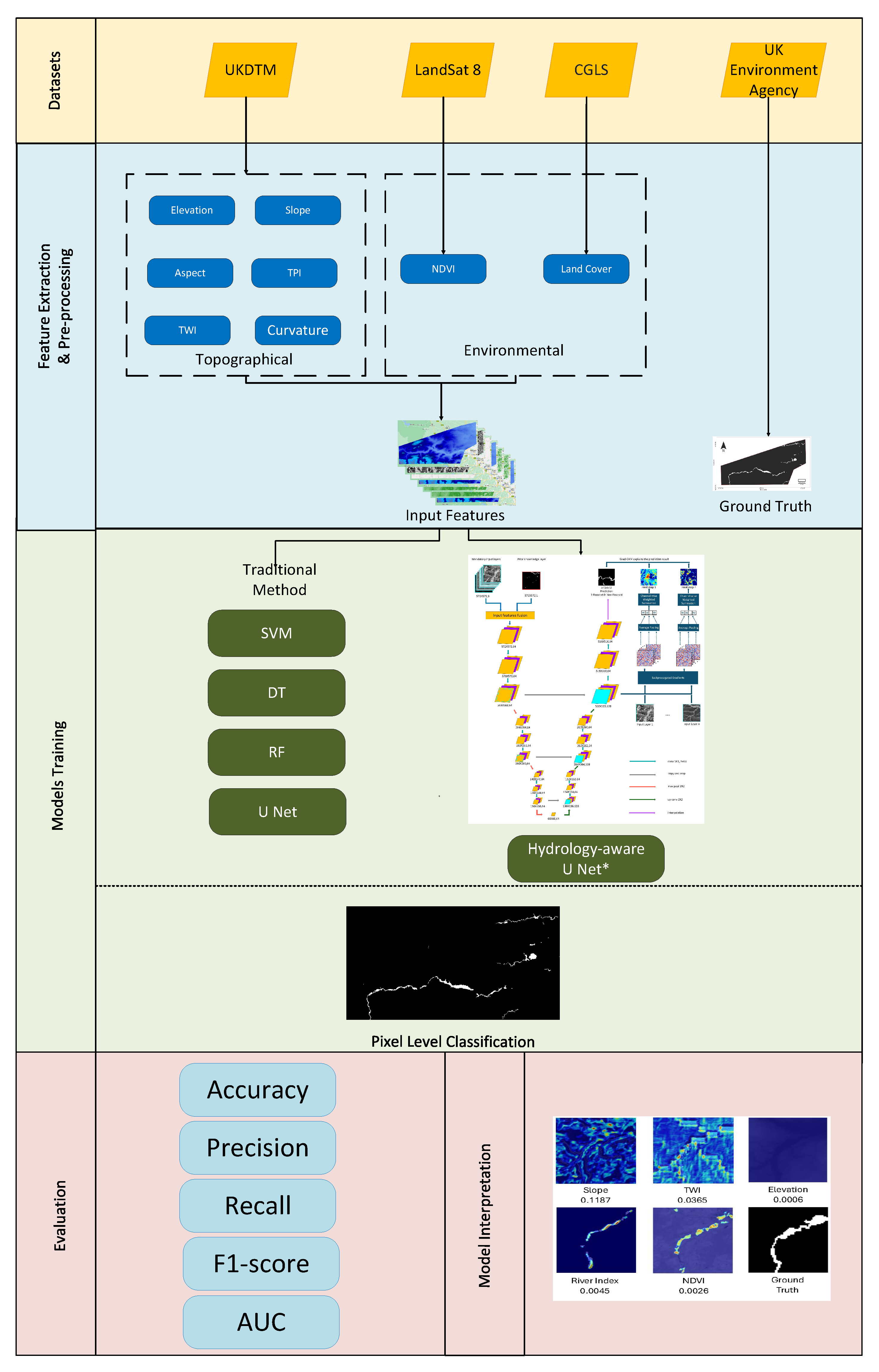
This study presents a comprehensive workflow for flood susceptibility mapping that integrates topographical, environmental, and hydrological features to enhance predictive accuracy. The workflow consists of three main stages, namely, (1) data preprocessing, (2) model training, and (3) evaluation. In the preprocessing stage, relevant flood susceptibility features—including terrain properties (elevation, slope), hydrological attributes (river proximity, drainage density), and land cover information—are extracted and formatted into both tabular and image-based representations to support different modelling approaches. To evaluate the effectiveness of deep learning-based flood susceptibility models, we implement a range of ML baselines, including SVM, decision trees (DTs), and RF. These models provide a benchmark for assessing spatial feature learning in contrast to convolution-based approaches. In addition, we train a standard U-Net architecture for pixel-wise flood susceptibility mapping. Finally, we introduce our hydrology-aware U-Net, which explicitly incorporates hydrological prior knowledge from river network data. Unlike conventional CNN-based models, which infer flood susceptibility solely from learned spatial correlations, our approach leverages hydrological priors to guide spatial feature extraction, improving generalisation within unseen parts of the study area. To enable interpretation of the model, we integrate Grad-CAM during the evaluation stage to provide a visual explanation of the features and regions most influential in driving model predictions.

2.1. Study Area

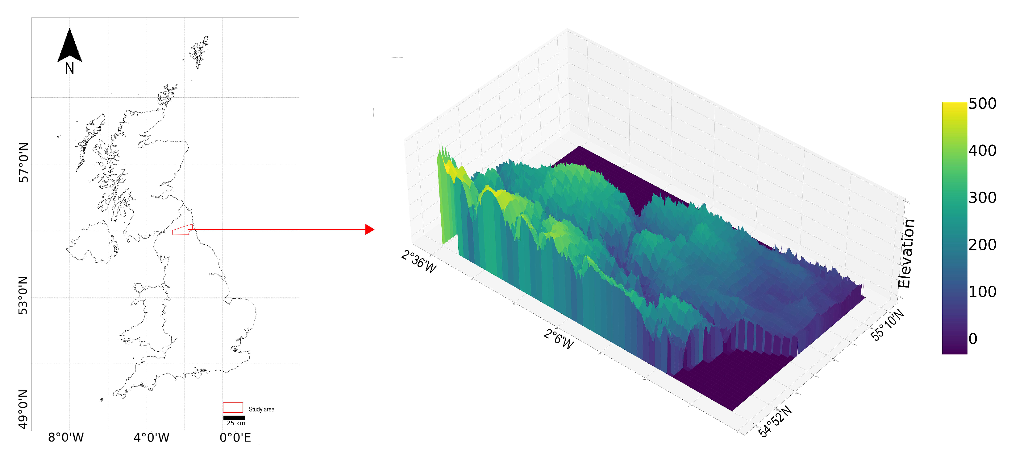
The study area, shown in Figure 1, is located in southern Northumberland, United Kingdom, covering approximately 1516 km². While this area is relatively small in scale, it contains diverse flood-prone landscapes—including river valleys, upland catchments, and peri-urban zones—allowing for robust evaluation of our method across multiple hydro-geomorphological settings within a controlled and computationally tractable environment. The terrain ranges from low-lying floodplains along the Tyne River (minimum elevation: −10 m) to upland areas reaching 602 m. The negative elevation values correspond to river channels and natural depressions prone to seasonal flooding. Human activities are primarily concentrated in the eastern lowlands, where sparse vegetation and urban expansion increase surface runoff potential. In contrast, the western uplands feature denser vegetation cover, steep slopes, and more permeable soil conditions, reducing flood risk but affecting runoff patterns. The predominant land cover types include farmlands, evergreen and deciduous forests, urban settlements, and sparsely vegetated zones—all of which play a role in modulating flood behaviour.

Hydrologically, the Tyne River is the dominant watercourse, flowing west to east and acting as a primary drainage system for the region. The river is highly responsive to intense rainfall events, with documented flooding events impacting communities along its banks. Additionally, the complex interplay between elevation, land cover, and river proximity makes this region particularly susceptible to localised and flash flooding. These physical drivers, combined with the area’s underrepresentation in prior remote sensing flood studies, make it well-suited for demonstrating the applicability and impact of deep learning-based flood susceptibility models in rural settings.

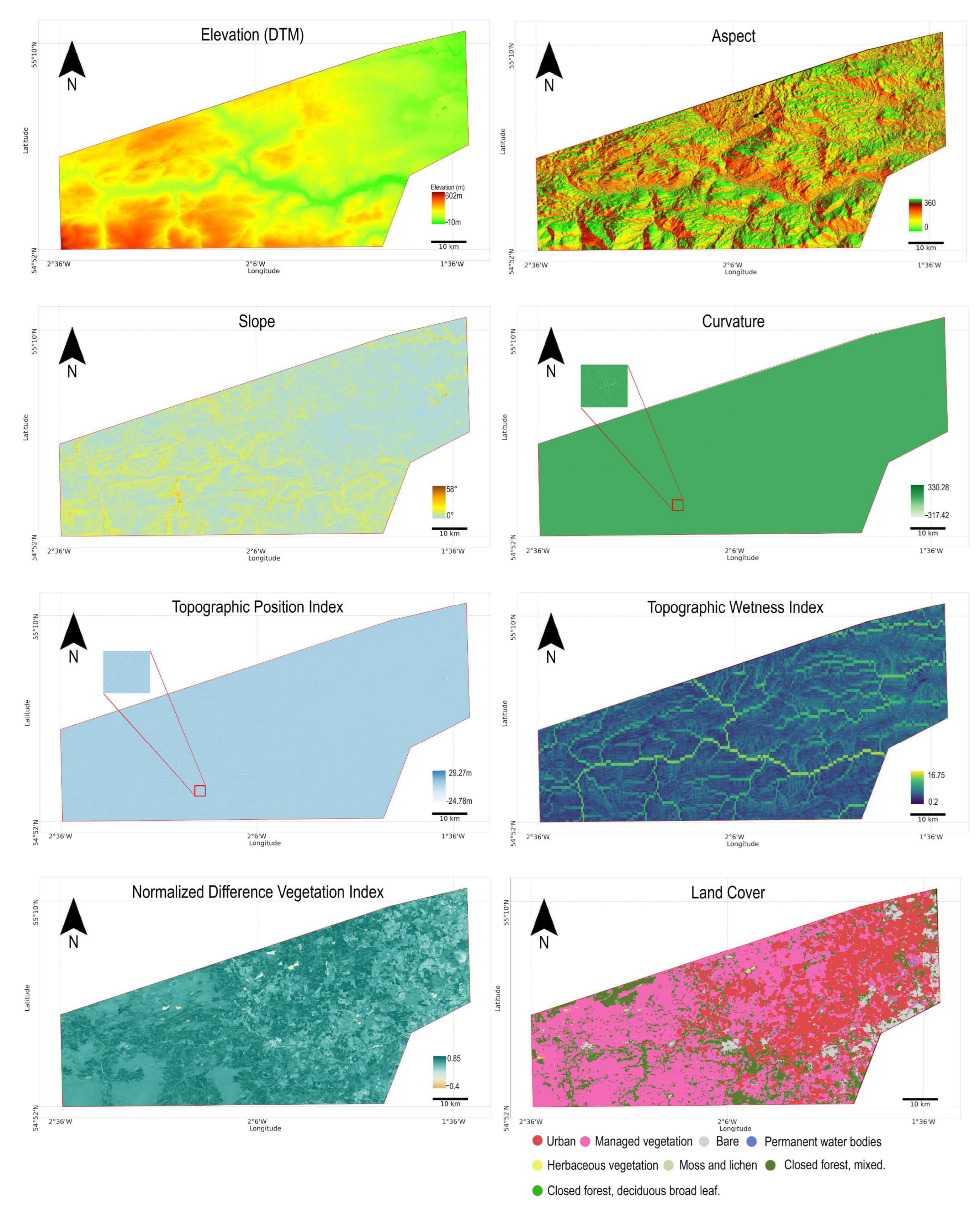
2.2. Flood-Influencing Factors

Flood susceptibility is influenced by a combination of topographical, environmental, and hydrological variables. Drawing on prior studies [31,32,33] and expert hydrological reasoning, we selected eight flood-influencing factors that collectively capture terrain morphology (e.g., elevation, slope, curvature), surface water accumulation (e.g., TWI, TPI), and land surface properties (e.g., NDVI, land cover, soil group). These factors were chosen based on their proven relevance in hydrological modelling and their complementary roles in describing runoff behaviour, infiltration, and water flow dynamics. Visual examples are provided in Figure 2, with sources and resolutions summarised in

Table 1. Features used in the present study. The resolution indicates that each pixel in the data image corresponds to an area of n × n meters on the ground.

	Feature	Resolution	Source	Range
1	Elevation	10 m	England 1 m Composite DTM	−34.27 m–604.68 m
2	Slope	10 m	England 1 m Composite DTM	$0^{\circ }$–${67.84}^{\circ }$
3	Aspect	10 m	England 1 m Composite DTM	$0^{\circ }$–${360}^{\circ }$
4	Curvature	10 m	England 1 m Composite DTM	−317.42 ${\mathrm{m}}^{-1}$–330.28 ${\mathrm{m}}^{-1}$
5	TPI	10 m	England 1 m Composite DTM	−24.78 m–29.27 m
6	TWI	10 m	England 1 m Composite DTM
		90 m	WWF HydroSHEDS Flow	0.2–16.75
			Accumulation
7	NDVI	30 m	USGS Landsat 8 Collection 2	−0.4–0.85
			Tier 1 TOA Reflectance
8	Land Cover	100m	Copernicus Global Land Cover	23 categories

.

Topographical and Environmental Factors

Topographical factors refer to the physical features of the Earth’s surface that influence flood susceptibility. These data are obtained from a digital terrain model (DTM), which captures the bare ground elevation, excluding vegetation and man-made structures. Environmental factors refer to the natural and human-influenced characteristics of an area that affect its susceptibility to flooding, including NDVI and land cover, which have been obtained from the USGS Landsat 8 satellite and Copernicus Global Land Service, respectively.

• Elevation: Represents terrain height, directly influencing floodwater accumulation and drainage.
• Slope: Controls surface runoff speed and water infiltration; lower slopes generally indicate higher flood susceptibility.
• Aspect: Reflects terrain orientation, affecting solar radiation, vegetation patterns, and indirectly, surface runoff conditions.
• Topographic Wetness Index (TWI): Quantifies areas prone to soil saturation and runoff accumulation, crucial for identifying flood-prone zones.
• Topographic Position Index (TPI): Highlights terrain positions (e.g., valleys or ridges), significantly influencing local flood risk.
• Curvature Index (CI): Describes terrain curvature, influencing runoff convergence (concave areas) or divergence (convex areas).
• Normalised Difference Vegetation Index (NDVI): Indicates vegetation coverage, affecting rainfall interception, infiltration, and runoff processes.
• Land Cover: Characterises land surface types (e.g., urban, vegetation), directly affecting runoff generation and infiltration capacity.

2.3. Hydrological Priors

In addition to the eight flood-influencing factors, our framework integrates prior knowledge of permanent river locations as an additional input. The river index map (Figure 3) serves as a form of prior hydrological knowledge, anchoring the model’s learning process in known, physically meaningful flood sources.

The use of river index maps is based on the well-established role of river-induced (fluvial) flooding, which is a dominant flood mechanism in many regions, including our study area. Unlike purely data-driven learning, this prior knowledge explicitly guides the model to pay attention to areas historically prone to overbank flow and channel overflow. This improves both performance and interpretability, ensuring that flood predictions are consistent with real-world hydrological behaviour.

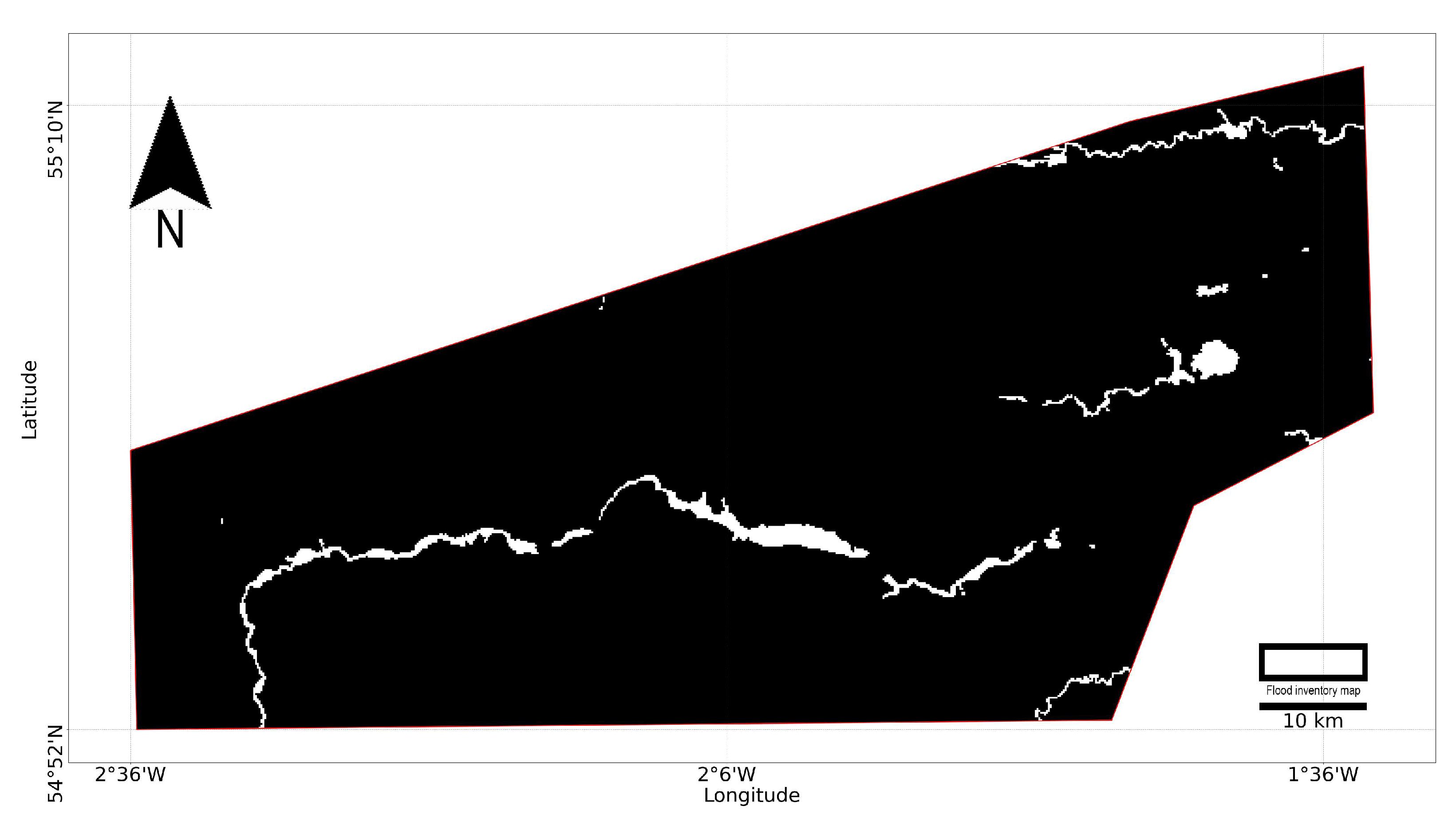
2.4. Flood Inventory Map

In our study, ground truth refers to the authoritative records of historical flood extents, which serve as the reference labels for training and evaluating flood susceptibility models. We utilise official flood records from the UK Environment Agency, which offers one of the most comprehensive publicly available flood databases (Environment Agency: https://www.gov.uk/government/organisations/environment-agency Accessed: 13 January 2025). The flood inventory dataset used in this study, shown in Figure 4, represents the maximum recorded extent of past flood events from rivers, coastal inundation, and groundwater springs, covering events from 1946 to the present. This dataset is well-suited for flood susceptibility modelling in our study, as it provides an extensive historical perspective on flood-prone regions. However, it should be acknowledged that it does not include surface water (pluvial) flooding. Since surface water is a major cause of urban flooding, particularly during short-duration intense rainfall, its absence may lead to an underestimation of flood susceptibility in densely populated areas.

2.5. Machine Learning Models

To evaluate different modelling approaches for flood susceptibility mapping, we employ a combination of traditional ML classifiers (SVM, DT, RF) and deep learning segmentation models (U-Net and modified U-Net). The ML classifiers serve as a benchmark for flood susceptibility classification using tabular feature representations, while U-Net is a widely used deep learning approach for spatially-aware flood prediction, capable of capturing complex flood patterns from remote sensing imagery.

2.5.1. Support Vector Machine

SVM is a kernel-based method which, in this context, transforms flood predictors into a higher-dimensional space, enabling better separation between flooded and non-flooded areas. SVM seeks to determine an optimal hyperplane capable of separating support vectors, in this case, flooded and non-flooded locations. A key advantage of SVM in flood susceptibility mapping is its ability to handle non-linear flood patterns, which are influenced by multiple environmental and hydrological factors [34]. Additionally, SVM is able to minimise test error while maintaining low model complexity.

The mathematical expression for classification with SVM is given as follows:

$$f\left(x\right)=\sum _{i=1}^n({\alpha }_i-{\alpha }_i^{*})K(x_i,x)+b,$$

(1)

where ${\alpha }_i$ and ${\alpha }_i^{*}$ denote the Lagrange multipliers, (${\alpha }_i\ge 0,{\alpha }_i^{*}\le C$), $K(x_i,x_j)$ represent the kernel functions, and b indicates the offset of the hyperplane from the origin.

2.5.2. Decision Tree

The DT algorithm is a widely used supervised learning method for flood susceptibility modelling due to its simplicity, interpretability, and ability to handle both numerical and categorical data. A DT works by recursively partitioning the feature space into distinct regions based on the threshold values of the input features. At each node, the algorithm selects a feature and a split point that minimises an impurity measure, such as the Gini index or entropy [35]. This process continues until a stopping criterion, such as a maximum depth or minimum number of samples per leaf node, is met. The final DT can be represented as a series of decision rules with the equation:

$$R_j=\{x\mid x_i\le t_j\}$$

(2)

where x represents the input features, $x_i$ is the selected feature, and $t_j$ is the threshold value for the split.

The main advantages of DT models include their ability to capture complex, non-linear relationships and provide an interpretable structure for decision-making. However, they are prone to overfitting, especially with noisy or imbalanced datasets, which can be mitigated using pruning techniques or ensemble methods such as RF and XGBoost.

2.5.3. Random Forest

The RF algorithm is an ensemble learning method that improves the performance and robustness of individual DTs by combining multiple trees into a single model [36]. RF reduces the risk of overfitting by introducing randomness during the training process, where each tree is constructed using a bootstrap sample of the original dataset, and feature selection for each split is limited to a random subset of input features. This process helps reduce the correlation between trees and improves generalisation.

For classification tasks, RF aggregates predictions from all trees through a majority vote for classification. The overall prediction can be expressed as follows:

$$\widehat{f}\left(x\right)={\displaystyle \frac{1}{B}}\sum _{b=1}^B{f}_b\left(x\right)$$

(3)

where $\widehat{f}\left(x\right)$ is the final prediction, B is the total number of trees, and $f_b\left(x\right)$ represents the prediction from an individual tree.

The key advantages of RF include its ability to handle high-dimensional datasets, capture complex non-linear relationships, and provide feature importance rankings to identify the most influential predictors. Additionally, RF is less sensitive to noisy data and class imbalance compared to single DTs. However, the trade-off is increased computational cost due to the ensemble nature of the model, which also makes the model less interpretable.

2.5.4. U-Net

U-Net is a deep learning algorithm designed for pixel-level image segmentation, with a symmetric encoder–decoder architecture. This structure enables the U-Net to capture contextual information at multiple scales while preserving spatial resolution, making it highly effective for tasks requiring pixel-level predictions [37].

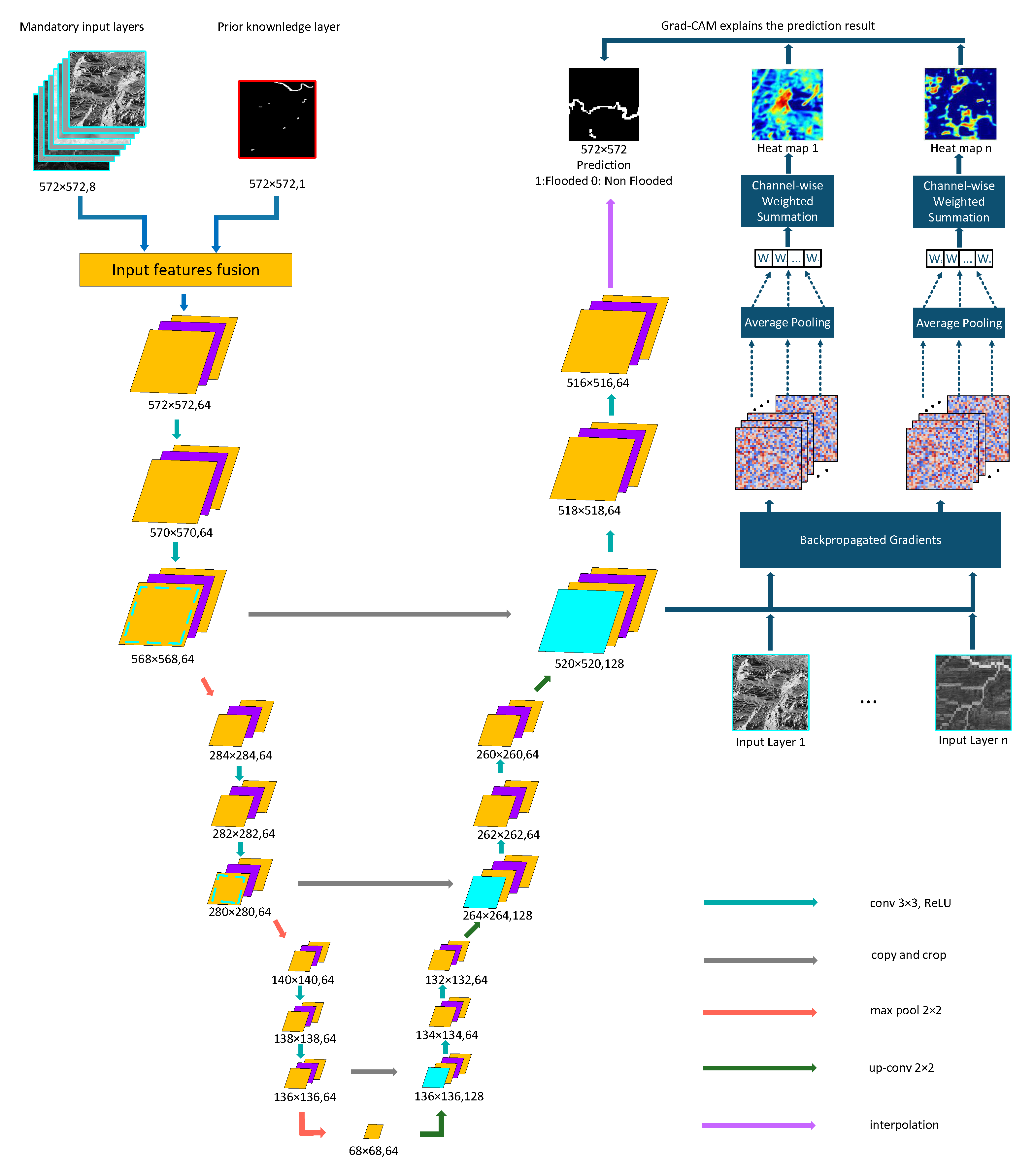
The encoder extracts hierarchical features from the input data through successive convolutional and pooling layers, similar to a traditional CNN. The decoder reconstructs the spatial information by up-sampling the extracted features and merging them with corresponding features from the encoder through skip connections, as depicted in Figure 5. These skip connections help retain fine-grained details lost during down-sampling, improving the accuracy of segmentation tasks.

The U-Net architecture combines low-level spatial information from the encoder with high-level contextual information from the decoder. Each layer of the U-Net employs convolutional operations, followed by non-linear activation functions (e.g., ReLU), which allow the network to learn complex patterns. The up-sampling layers in the decoder use transposed convolutions to restore the resolution of the feature maps.

To improve hydrologically meaningful flood predictions, we introduce a modified U-Net architecture that incorporates river network data as a prior knowledge feature. Unlike standard U-Net, which learns flood patterns purely from spatial correlations, this modification explicitly encodes hydrological constraints, allowing the model to focus on flood-prone regions associated with river networks. The river index map is added as an additional input channel, ensuring that the encoder extracts hydrological patterns from the earliest layers. This approach allows the model to learn spatial dependencies between rivers and surrounding terrain, improving prediction robustness in areas where topographic and environmental factors alone may be insufficient.

2.6. Model Interpretation with Grad-CAM

Explainability is a critical aspect of flood susceptibility modelling, as predictive models must not only yield accurate flood risk assessments but also provide transparent and interpretable insights for disaster management and policy decisions [38]. To address this challenge, we employ gradient-weighted class activation mapping (Grad-CAM), an explainability technique that highlights the most influential regions in the model’s decision-making process. Grad-CAM generates heatmaps overlaying the input image, showing which spatial regions contribute most to the model’s prediction of flood susceptibility. This helps to answer key questions about the model, such as whether the model focuses on relevant regions or if predictions are influenced by irrelevant artefacts, as well as the extent to which flood-influencing factors contribute to the flood susceptibility classification.

Grad-CAM provides visual explanations by computing the gradients of the target class $y_c$ (flooded or not flooded), with respect to feature map activations $A^k$, from intermediate convolutional layers, computed as follows:

$$L_c^{\mathrm{Grad}-\mathrm{CAM}}=\mathrm{ReLU}\left(\sum _k{\alpha }_k^c{A}^k\right)$$

(4)

$${\alpha }_k^c={\displaystyle \frac{1}{Z}}\sum _{i,j}{\displaystyle \frac{\partial y_c}{\partial A_{ij}^k}}$$

(5)

where ${\alpha }_k^c$ represents the importance weight of the feature map k, and is the total number of pixels in the feature map. We apply Grad-CAM to the final convolutional layers of U-Net’s encoder, as this stage contains high-level spatial representations of flood risk. The generated heatmaps allow us to interpret whether the model is correctly attending to hydrologically relevant areas.

2.7. Experiments

In this study, we design a multi-stage experimental pipeline to evaluate the effectiveness of our integration of hydrological priors into flood susceptibility mapping. The process begins with the extraction and preprocessing of topographical, environmental, and hydrological data, which are formatted to support both traditional machine learning models and deep learning architectures. We implement and compare baseline models, including SVM, DT, RF, and a standard U-Net, against our proposed hydrology-aware U-Net that explicitly incorporates prior knowledge of river networks. Each model is trained and evaluated using a consistent dataset and assessed using a range of performance metrics, including accuracy, precision, recall, F1 score, and AUC. Grad-CAM is employed to interpret the behaviour of our hydrology-aware U-Net, providing both a quantitative assessment of feature importance and a visual analysis of the model’s spatial attention. This unified framework allows us to rigorously compare model performance and interpretability across approaches, as illustrated in Figure 6.

2.7.1. Data Preprocessing

To accommodate different ML model architectures, our dataset is prepared in the following formats: (1) tabular data format, which represents flood-influencing factors as numerical features for use in traditional classifiers such as SVM, DT, and RF, and (2) image data format, which maintains the spatial structure of flood susceptibility patterns for use in deep learning models such as CNNs and U-Net.

Each pixel (or corresponding data point in the tabular data) is assigned a binary label based on the flood inventory map, where historically flooded areas are labelled as ‘flooded’ (1) and non-flooded areas as ‘non-flooded’ (0). Flood inventory polygons were rasterised before model training to ensure label consistency across formats.

Class imbalance is a well-known challenge in flood susceptibility modelling, where the majority of the study area consists of non-flooded regions. In our dataset, approximately 97.6% of pixels are labelled as non-flooded, which can bias the model toward over-predicting the dominant class. To mitigate this, we adopt a patch-based sample selection strategy in which only image patches containing at least 10% flooded pixels are retained for training.

This 10% threshold was determined based on both prior experience and empirical evaluations of multiple cutoff values (e.g., 1%, 5%, 10%, 20%). Lower thresholds yielded an excessive number of highly imbalanced patches, while higher thresholds significantly reduced the total number of training samples. The 10% setting provides the best trade-off by ensuring that flood-prone areas are adequately represented without sacrificing dataset size. Using this threshold, we obtained 29,677 patches, which were split into 80% for training and 20% for testing. To further examine the spatial generalisation ability of the proposed method, we conduct a spatial 5-fold cross-validation. In this procedure, the study area was divided into five geographically distinct subsets (folds). In each iteration, one fold serves as the test set while the remaining four are used for training. This process is repeated five times to ensure that each fold is evaluated independently.

To maintain spatial consistency, we applied a sliding window with a size of 572 × 572 pixels and a stride of 10 pixels. This window size was selected based on empirical testing to balance the trade-offs between spatial resolution, computational efficiency, and the receptive field of the model. The 10-pixel stride introduces sufficient overlap between adjacent patches, improving generalisation by exposing the model to slight variations in spatial context. The selected dataset is represented in Figure 7.

Raw datasets were obtained from Google Earth Engine (GEE) in GeoTIFF format, with 10 m resolution across all features. To ensure compatibility across models, the data are formatted accordingly. For CNN models, the data are converted to PNG format, ensuring spatial consistency and efficient processing. For the ML models, pixel values are extracted and stored in CSV format, where each row represents a single pixel with its corresponding feature values.

To integrate hydrological priors into the deep learning pipeline, we treat the river index map as a separate input channel alongside the eight other features. This design ensures that the spatial signal from the river network influences all layers of the U-Net architecture, rather than being fused at deeper stages. This approach preserves spatial alignment and enables the model to learn hydrologically grounded feature representations from the earliest stages of training.

2.7.2. Model Training

This study aims to evaluate the effectiveness of incorporating spatial context and prior hydrological knowledge into flood susceptibility mapping. Specifically, we investigate two key aspects: (1) the extent to which capturing spatial dependencies through a U-Net architecture enhances predictive performance compared to traditional ML classifiers such as SVM, DT, and RF; and (2) the impact of explicitly integrating river network data as prior knowledge into deep learning models.

To address these objectives, we compare our proposed approach against representative baselines from recent literature. These include SVM [39], DT [8], and RF [40], each implemented and evaluated under consistent conditions. For all traditional ML models, basic hyperparameter tuning was conducted using grid search with cross-validation. For the SVM, we tuned the penalty parameter C and tested different kernel types (e.g., linear and RBF). For the DT, we optimised parameters such as maximum tree depth and minimum samples per split. For the RF, the number of estimators and maximum depth were adjusted based on validation performance. All models were trained and validated on the same data splits to ensure a fair and consistent comparison. We also include a standard U-Net as a deep learning baseline to evaluate the added value of hydrological priors in our proposed variant.

For deep learning models, input images are extracted into patches of 572 × 572 pixels, ensuring consistency with U-Net’s input size requirements, while for traditional ML models (SVM, DT, RF), feature values are extracted from each pixel and converted into a tabular format. We evaluate our model using the hold-out validation method, so the datasets are split into train and test sets with a ratio of 80:20. The same data split is applied to both datasets to ensure fair comparisons between classical ML and deep learning approaches.

To improve the hydrological fidelity of flood susceptibility prediction, we propose a modified U-Net architecture that integrates domain-specific prior knowledge in the form of a river network index map. While the standard U-Net architecture relies solely on spatial feature learning from topographic and environmental inputs, our enhanced design incorporates a hydrologically meaningful guidance mechanism via early fusion.

In this design, a binary river index map is concatenated with the input feature stack as an additional channel, expanding the input tensor dimensionality from C to $C+1$. This early fusion strategy enables the encoder to integrate raw hydrological priors directly into the low-level convolutional feature extraction process, as opposed to late fusion methods, which typically inject such information into higher layers or through auxiliary heads. By embedding the river network at the input level, the network conditions its convolutional filters to attend to flood-relevant spatial structures from the first layer, effectively biasing the learned feature representations toward hydrologically plausible regions.

This mechanism is particularly important given the spatially structured nature of flood phenomena, where hydrodynamic processes often propagate along river corridors. Early fusion allows these spatial dependencies to be encoded hierarchically as features propagate through deeper layers, influencing both local receptive field activations and global context aggregation. Furthermore, it implicitly introduces a spatial prior that helps regularise feature learning in areas where traditional topographic or environmental predictors (e.g., NDVI, slope) are ambiguous or noisy. This tight integration between raw data and domain knowledge promotes better generalisation and interpretability.

Architecturally, our model retains the symmetric encoder–decoder structure and skip connections of the original U-Net, preserving the multi-scale spatial learning capability. However, the incorporation of early-fused hydrological priors fundamentally reorients the feature extraction process, resulting in enhanced discrimination between flood-prone and non-flooded regions, as demonstrated in the experimental results.

The U-Net models are implemented with PyTorch 3.12 on an NVIDIA A100 GPU (NVIDIA, Santa Clara, CA, USA) to ensure efficient computation. We optimise the training process with Adam, with an initial learning rate of 0.001, which is dynamically adjusted using the ReduceLROnPlateau scheduler. This scheduler reduces the learning rate to 10% of its current value if the validation loss plateaus for 10 consecutive epochs. During optimisation, we minimise the binary cross-entropy (BCE) loss, which measures the dissimilarity between the predicted probabilities and the true binary labels, making it suitable for pixel-level binary segmentation tasks. It penalises predictions that deviate from the ground truth, encouraging the model to output probabilities close to the true class labels.

The BCE loss for a single pixel prediction p and its corresponding ground truth label y is defined as follows:

$${\mathcal{L}}_{\mathrm{BCE}}=-\left[y·log\left(p\right)+(1-y)·log(1-p)\right]$$

(6)

where $y\in \{0,1\}$ is the ground truth label (0 for non-flood, 1 for flood), $p\in [0,1]$ is the predicted probability for the positive class, and log denotes the natural logarithm.

For a batch of N pixel predictions, the BCE loss is averaged across all pixels as follows:

$${\mathcal{L}}_{\mathrm{BCE}}=-{\displaystyle \frac{1}{N}}\sum _{i=1}^N\left[y_i·log\left(p_i\right)+(1-y_i)·log(1-p_i)\right]$$

(7)

where $y_i$ and $p_i$ represent the ground truth label and predicted probability for the i-th pixel, respectively.

The BCE loss effectively handles imbalanced data by ensuring that predictions for both the foreground (flood) and background (non-flood) classes contribute proportionally to the loss. By minimising this loss function, the U-Net model learns to predict pixel-wise probabilities that align with the true flood mask, improving segmentation accuracy.

2.7.3. Evaluation

Model performance is evaluated using several widely accepted statistical metrics, including accuracy, precision, recall, F1 score, and AUC. These metrics provide a comprehensive assessment of the classification quality and discrimination capability of the models, and are computed as follows:

• Accuracy: Measures the overall fraction of correct predictions, and is computed as follows:

  $$\mathrm{Accuracy}={\displaystyle \frac{\mathrm{TP}+\mathrm{TN}}{\mathrm{TP}+\mathrm{FP}+\mathrm{TN}+\mathrm{FN}}}$$

  (8)

  where TP, TN, FP, and FN are true positive, true negative, false positive, and false negative, respectively.
• Precision: Indicates the proportion of predicted flood-prone pixels that are actually flood-prone, highlighting the model’s ability to avoid false positives, computed as follows:

  $$\mathrm{Precision}={\displaystyle \frac{\mathrm{TP}}{\mathrm{TP}+\mathrm{FP}}}$$

  (9)
• Recall: Represents the proportion of actual flood-prone pixels correctly identified by the model, emphasising its ability to capture true positives and avoid false negatives, and is computed as follows:

  $$\mathrm{Recall}={\displaystyle \frac{\mathrm{TP}}{\mathrm{TP}+\mathrm{FN}}}$$

  (10)
• F1 score: Represents the harmonic mean of precision and recall, providing a balanced evaluation metric especially suitable when dealing with imbalanced datasets, and is computed as follows:

  $$\mathrm{F}1\mathrm{score}=2\times {\displaystyle \frac{\mathrm{Precision}\times \mathrm{Recall}}{\mathrm{Precision}+\mathrm{Recall}}}$$

  (11)
• AUC: Measures the model’s ability to distinguish between flooded and non-flooded pixels across all possible classification thresholds. It is particularly useful for imbalanced datasets and is computed as the area under the receiver operating characteristic (ROC) curve:

  $$\mathrm{AUC}={\int }_0^1\mathrm{TPR}d\mathrm{FPR}\approx \sum _{i=1}^{n-1}({\mathrm{FPR}}_{i+1}-{\mathrm{FPR}}_i)·{\displaystyle \frac{{\mathrm{TPR}}_{i+1}+{\mathrm{TPR}}_i}{2}}.$$

  (12)

  where TPR is the true positive rate and FPR is the false positive rate; it is computed as follows:

  $$\mathrm{TPR}={\displaystyle \frac{\mathrm{TP}}{\mathrm{TP}+\mathrm{FN}}}$$

  (13)

  $$\mathrm{FPR}={\displaystyle \frac{\mathrm{FP}}{\mathrm{FP}+\mathrm{TN}}}$$

  (14)
  AUC ranges from 0 to 1, where 1 denotes perfect discrimination and 0.5 indicates random guessing. It is particularly suitable for imbalanced datasets, as it evaluates classification performance independently of the decision threshold. In this study, AUC is computed at the pixel level for traditional classifiers and deep learning models. In flood susceptibility prediction, AUC is particularly advantageous because it is robust to class imbalance, a common challenge for this task.

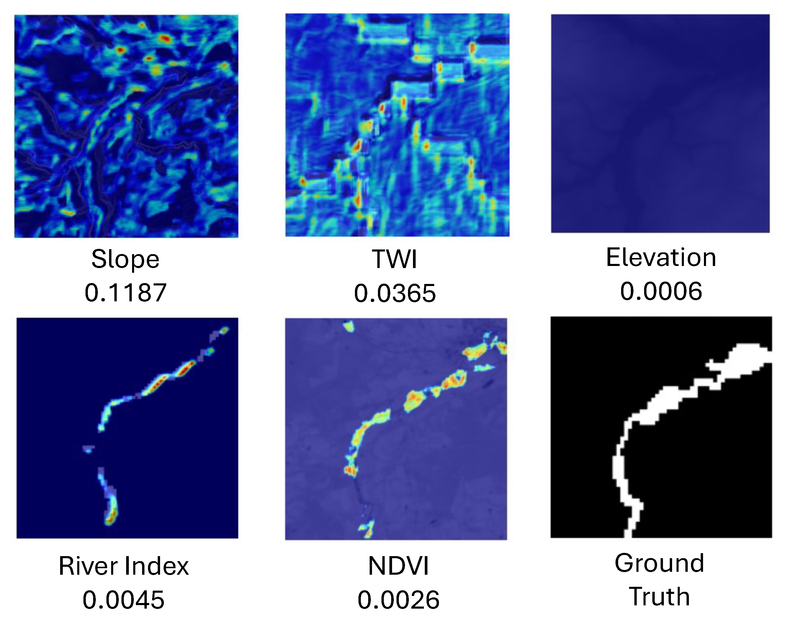
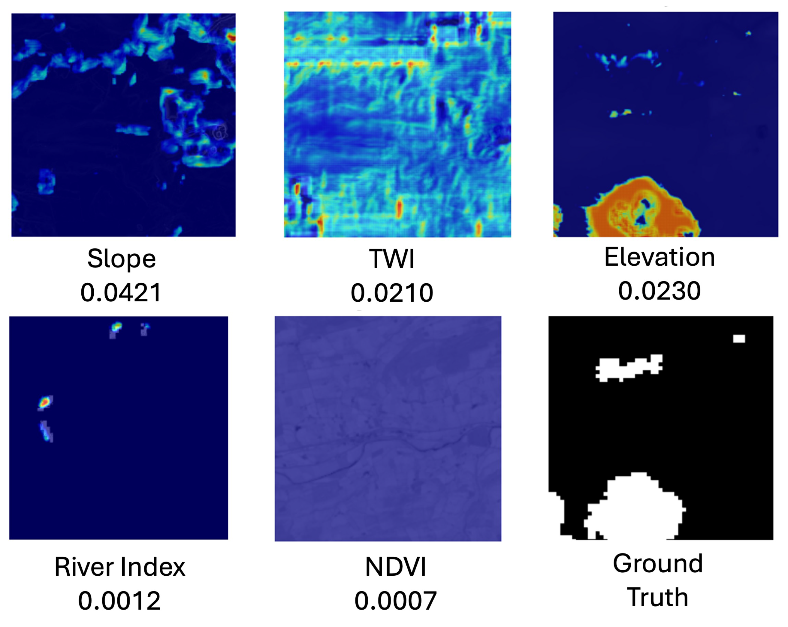
In addition to standard performance metrics, we evaluate the interpretability of the hydrology-aware U-Net using Grad-CAM. To isolate the contribution of each input feature, we apply Grad-CAM in a channel-wise manner by masking all but one input layer at a time. This generates per-feature attribution maps, allowing both global and local analysis of feature influence. For global importance, we compute the average, standard deviation, and maximum Grad-CAM weights for each feature across the test set. To examine spatial attention, we visualise the resulting attribution maps alongside their corresponding average attribution scores, providing qualitative insight into how the model prioritises different features under varying flood scenarios.

3. Results

3.1. Performance Analysis

The performance of each flood susceptibility model is presented in

Table 2. Performance comparison of traditional and deep learning models across key classification metrics.

Model	Accuracy	Precision	Recall	F1 score	AUC
DT	0.63	0.48	0.52	0.50	0.554
SVM	0.67	0.53	0.58	0.55	0.616
RF	0.70	0.59	0.63	0.61	0.684
U_NET	0.93	0.76	0.84	0.80	0.931
Proposed method	0.96	0.79	0.86	0.82	0.966

, with corresponding AUC curves shown in Figure 8. The proposed hydrology-aware U-Net achieves the best overall performance, with an accuracy of 0.96, a precision of 0.79, a recall of 0.86, an F1 score of 0.82, and an AUC of 0.966. The standard U-Net also performs well, achieving an AUC of 0.931, but shows lower precision and recall compared to the proposed model. In contrast, the traditional ML models demonstrate substantially weaker performance across all metrics. Figure 9 provides a visual illustration of a prediction from our proposed model compared to the ground truth for a sample test patch. As shown in the rightmost panel, the model accurately detects the flooded region, with relatively few misclassified pixels, and makes relatively few incorrect pixel classifications.

Table 3. Performance metrics of the U_Net with prior knowledge model across spatial 5-fold cross-validation. Each fold represents a geographically distinct subset of the study area. The results include accuracy, precision, recall, F1 score, and AUC. The final row reports the mean and standard deviation across folds, reflecting the model’s consistency and generalisation capability across different geographic contexts.

Fold	Accuracy	Precision	Recall	F1 Score	AUC
1	0.9636	0.7598	0.8382	0.7970	0.9809
2	0.9536	0.7083	0.8101	0.7802	0.9500
3	0.9598	0.7350	0.8281	0.7888	0.9662
4	0.9750	0.7617	0.8401	0.8012	0.9883
5	0.9604	0.7428	0.8277	0.7836	0.9724
Mean	0.9625	0.7415	0.8288	0.7902	0.9716
Std	0.0079	0.0217	0.0119	0.0088	0.0147

summarises the spatial 5-fold cross-validation results for our model, offering insight into its generalisation capabilities across geographically distinct areas. The model exhibits consistently strong performance across all five folds, achieving an average accuracy of 0.9625, a precision of 0.7415, a recall of 0.8288, and an F1 score of 0.7902. Additionally, the mean AUC score of 0.9716 further highlights the model’s strong capability in distinguishing between flood-prone and non-flood-prone areas.

The loss curves for the two U-Net models shown in Figure 10 clearly demonstrate the impact of incorporating explicit prior knowledge into the input data. The graphs show that our proposed hydrology-aware U-Net demonstrates better performance from the start of training, where the training loss drops from 1.233 in the standard U-Net to 0.9864 in the U-Net with prior knowledge. The rapid loss reduction further highlights the training efficiency of the U-Net with prior knowledge compared to the standard U-Net. Using a loss of 0.45 as a reference threshold, the proposed model achieves this value within approximately 7 epochs (approximately 49 min), while the standard U-Net takes nearly 87 epochs (approximately 609 min) to reach the same level, approximately a 90% improvement.

The speed to reach steady-state loss further emphasises the efficiency of the U-Net with prior knowledge. Our model stabilises its training and validation losses within approximately 50 epochs, whereas the standard U-Net requires nearly 150 epochs to achieve a similar level of stability.

3.2. Interpretation with Grad-CAM

To interpret the model’s decision-making, enabling assessment of whether the model learns hydrologically meaningful patterns, we apply Grad-CAM to the final encoder layer of the trained hydrology-aware U-Net. To identify which features contribute most to the model’s flood susceptibility predictions, we compute the average and maximum Grad-CAM weights across the test set, as shown in

Table 4. The average weight, standard deviation, and maximum weight from the Grad-CAM attributions across the testing portion of the dataset.

Feature	Average Weight	Standard Deviation	Maximum Weight
Elevation	0.0093	0.0073	0.0431
Slope	0.0865	0.0274	0.1127
Aspect	0.0001	0.0002	0.0018
Curvature	0.0001	0.0002	0.0015
TWI	0.0050	0.0012	0.0091
TPI	0.0003	0.0005	0.0035
NDVI	0.0019	0.0007	0.0036
Land Cover	0.0001	0.0002	0.0015
River Index	0.0040	0.0012	0.0073

, and show their ranking in Figure 11. These weights reflect how strongly each input layer influenced the model’s classification decisions.

The results clearly show that slope is the most influential feature, with an average attribution weight of 0.0865, followed by TWI (Topographic Wetness Index), which also receives substantial attention from the model. The hydrological prior, river index, shows moderate but consistent importance, suggesting that the model leverages this spatial prior as a useful anchor for guiding flood predictions. The remaining features, including elevation, TPI, aspect, and vegetation-related variables (NDVI, land cover), exhibit very low average attribution weights. However, the maximum values for elevation and TPI indicate that these features may still play an important role in specific instances.

To better understand how the model’s reliance on input features varies across different flood scenarios, Figure 12 and Figure 13 illustrate Grad-CAM attribution maps for two representative test samples. In these figures, we exclude the aspect, curvature, TPI, and land cover, as their activations are close to zero in both samples and are not visually meaningful. In Figure 12, the flooded region coincides with a permanent water body. Here, the River Index and NDVI exhibit strong spatial attribution, indicating the model is leveraging hydrological priors and vegetation cues to detect fluvial flood risk. In contrast, Figure 13 shows a flooded region with no nearby permanent water body. In this case, elevation is the dominant feature, suggesting the model relies more heavily on topographic depressions to identify flood-prone areas. In both samples, both slope and TWI show the highest activations, but the attention is much less focused on the flooded region, with slope showing scattered activations, particularly in areas with terrain transitions or edges, and TWI showing widespread, banded activation, with areas with higher TWI values showing greater activation levels. These examples demonstrate the model’s adaptive feature prioritisation depending on the local hydrological context, supporting the utility of integrating priors while maintaining generalizability to diverse flood mechanisms.

4. Discussion

The performance gap observed between traditional ML models and deep learning-based approaches can be largely attributed to their respective data representations. While conventional models rely on tabular summaries, which ignore spatial structure, U-Net models process full-resolution spatial data, enabling them to capture complex spatial dependencies associated with flood susceptibility.

These results align with previous studies that demonstrate the superiority of deep learning models for flood risk mapping [41,42]. However, our results further emphasise the importance of incorporating prior hydrological knowledge. The proposed hydrology-aware U-Net consistently outperforms the standard U-Net, achieving a 3.5-point improvement in AUC and higher precision and recall. This suggests that embedding domain knowledge into the learning process enhances the model’s ability to detect flood-prone areas beyond what is possible with data-driven learning alone.

The model’s strong generalisation capability is further supported by the 5-fold spatial cross-validation results, which show consistently high accuracy and AUC across geographically distinct subsets. These results reinforce the robustness of our approach across varied local terrain and hydrological contexts within the study area.

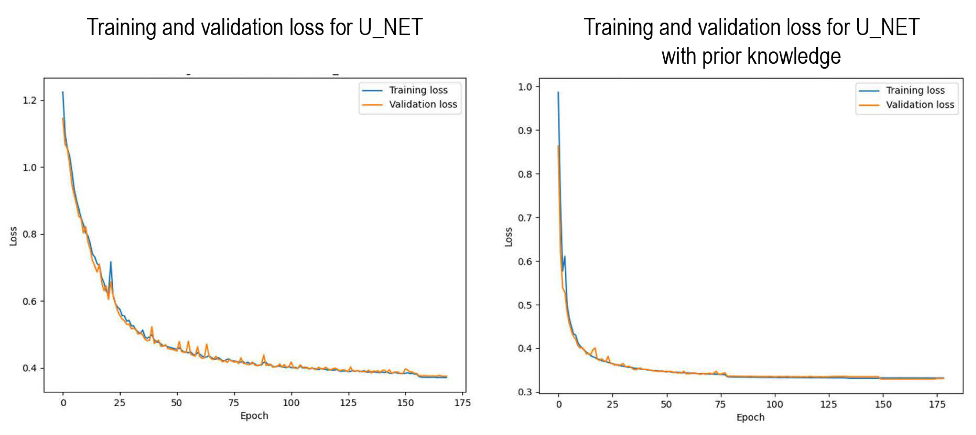
In addition to improved predictive performance, the training efficiency of the hydrology-aware model was significantly higher. The proposed model reaches a reference loss of 0.45 in just 7 epochs, compared to 87 epochs for the standard U-Net. It also converges to a stable learning state three times faster, indicating that hydrological priors act as a useful structural bias, guiding the model towards relevant patterns earlier in training.

Our Grad-CAM-based analysis revealed that slope and TWI received the highest attribution weights, indicating their dominant influence on flood susceptibility predictions. These findings are consistent with the empirical results of Al-Kindi and Alabri [43], who identified slope, TWI, elevation, and NDVI as critical flood-conditioning variables across multiple machine learning models. Their study, conducted in a fluvial landscape in Oman, reinforces the importance of these topographical and environmental factors in rural flood risk assessment. Additionally, in [44], slope and TWI were again among the most important flood conditioning factors. The alignment between Grad-CAM spatial attributions and these well-established flood predictors provides confidence in the interpretability and reliability of our deep learning model’s decisions.

While slope and TWI dominate on average, elevation and NDVI show important localised influence. NDVI appears to be particularly important in areas adjacent to rivers (e.g., Figure 12), likely because the model has learned to associate low vegetation cover with river channels or flood-prone corridors. In rural regions such as our study area, riverbanks often exhibit sparse vegetation due to scouring, erosion, or regular inundation. These low NDVI values provide a strong visual cue that helps the model distinguish natural drainage paths from surrounding vegetated terrain. Thus, NDVI serves not only as an indicator of surface characteristics but also as a useful proxy for identifying fluvial flood susceptibility in river-adjacent areas. Elevation plays a stronger role in samples without nearby permanent water bodies (e.g., Figure 13), where the model appears to rely on depressions in terrain to infer flood susceptibility, which is consistent with studies where elevation has been observed as a key variable in flood prediction [29,45].

Although this study focuses exclusively on Northumberland County, the proposed method is designed with generalizability in mind. The integration of prior knowledge is achieved through the use of a permanent waterbody index, a widely available and conceptually simple representation of river network structure. This prior does not rely on region-specific physical models or empirical thresholds, making it potentially transferable to other areas where similar hydrological data are available. However, it should be acknowledged that this study focuses on flood susceptibility in rural areas, where fluvial flooding is the dominant hazard due to the proximity to rivers. As such, both the ground truth and the hydrological prior are designed to capture fluvial flood patterns. However, this setup does not account for pluvial flooding, which is a significant contributor to flood risk in urban areas. While the proposed framework of integrating hydrological prior knowledge is conceptually generalisable, future work should explore adapting it to urban contexts, which will require both revised ground truth data and alternative forms of prior knowledge, such as drainage capacity or urban runoff models. Additionally, while the river index map provides a meaningful, low-complexity hydrological constraint, it captures only one aspect of flood generation. Future work could explore incorporating additional hydrological priors either at the input level or within the network architecture. Such extensions could improve model robustness across diverse flood scenarios while preserving interpretability and domain alignment.

Beyond static priors, an important avenue for future exploration involves integrating outputs from physics-based flood simulations, such as those generated by HEC-RAS or LISFLOOD, as additional input channels or supervisory signals. These simulations offer high-resolution representations of inundation extent, flow depth, or velocity, which can complement learning-based methods with physically grounded insights. In such cases, careful attention should be paid to how the underlying simulation is meshed, as spatial alignment between simulation grids and model inputs is essential for preserving geospatial fidelity. This integration may also require balancing the trade-off between physical realism and computational tractability, depending on the spatial resolution and coverage of the simulation outputs.

Furthermore, while the overall model architecture is flexible, performance in new regions is likely to benefit from retraining or fine-tuning on local data to account for variations in topography, land use, and hydrological behaviour. As such, while the model shows strong spatial generalisation within the study area, future work should evaluate its transferability across different climatic and geomorphological contexts. Finally, this study uses static input features such as topography, land cover, and vegetation, which are effective for long-term susceptibility mapping. However, it does not capture short-term temporal factors like rainfall intensity or soil saturation. Incorporating time-series data and adopting spatio-temporal architectures could enable event-based flood prediction and support applications in real-time forecasting or climate-sensitive risk assessment.

Despite these limitations, the proposed method has promising application prospects in regions where conventional flood forecasting tools are unavailable or impractical, particularly in data-sparse areas. Its reliance on widely available topographic and land cover data, combined with lightweight integration of hydrological priors, makes it well-suited for supporting flood risk mapping in underserved communities. The model’s strong performance and fast convergence also support operational deployment, including integration into early warning systems and local planning workflows. Importantly, the inclusion of Grad-CAM-based explainability enables domain experts and decision-makers to validate predictions and ensure transparency, making the framework particularly relevant for policy-facing applications such as resilience planning, land use regulation, or insurance risk assessments.

5. Conclusions

This study introduces a novel approach to flood susceptibility mapping that integrates spatial priors into deep learning models, demonstrating the importance of hydrological knowledge in enhancing predictive accuracy. By leveraging ML (SVM, DT, RF) and deep learning models (U-Net, modified U-Net), we assess how different modelling approaches perform in a 1516 km² region of Northumberland, UK. The results demonstrate that deep learning models significantly outperform tabular ML models, reinforcing the importance of spatial context in flood prediction. Incorporating hydrological priors improves both accuracy and training efficiency. The modified U-Net converges three times faster than the standard U-Net, demonstrating that explicitly embedding domain knowledge enhances model learning. Explainability through Grad-CAM reveals model reliance on topographical and environmental factors. The model correctly identifies low-lying regions and high TWI areas as flood-prone but also exhibits potential biases in NDVI-based river detection and aspect-dependent predictions. This study provides a robust and adaptable framework that can be extended to other environmental and disaster management applications where prior knowledge plays a pivotal role in improving model performance, interpretability, and training efficiency.