
MRCS-Net: Multi-Radar Clustering Segmentation Networks for Full-Pulse Sequences


Abstract

1. Introduction
- We proposed a deep learning framework for full-impulse signal segmentation clustering, which establishes a breakthrough in full-pulse clustering orientation and demonstrates enhanced accuracy compared to traditional single-pulse clustering approaches.
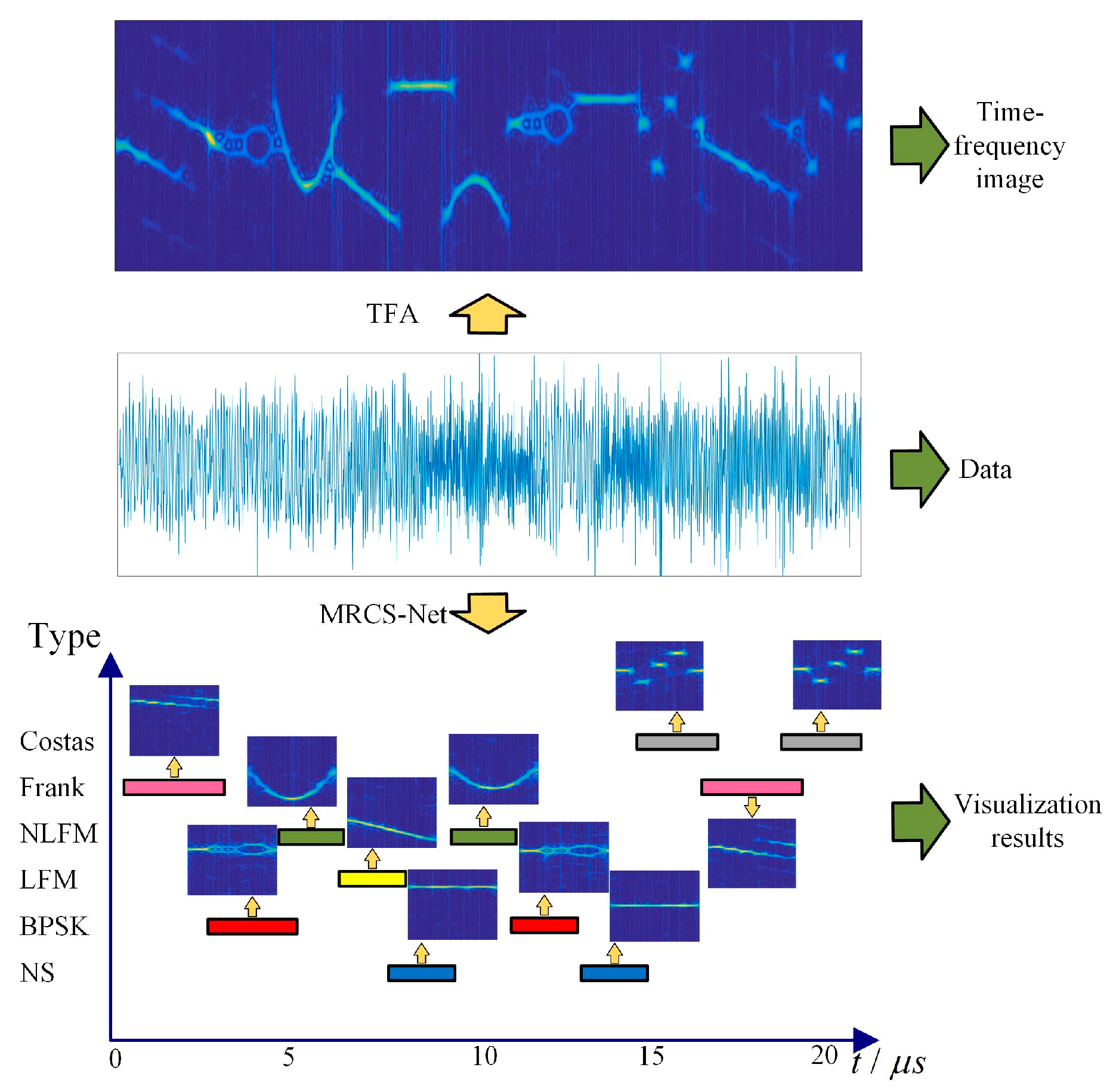
- We integrated a SincNet subnetwork and a pulse activity detection subnetwork. The SincNet network performs the signal filtering process, and the impulse activity detection network implements the signal clustering and recognition.
- Extensive experiments show that our proposed method has excellent performance for processing long-time full-pulse sequences. Our model achieved excellent results on segmentation error rate and recognition accuracy metrics.
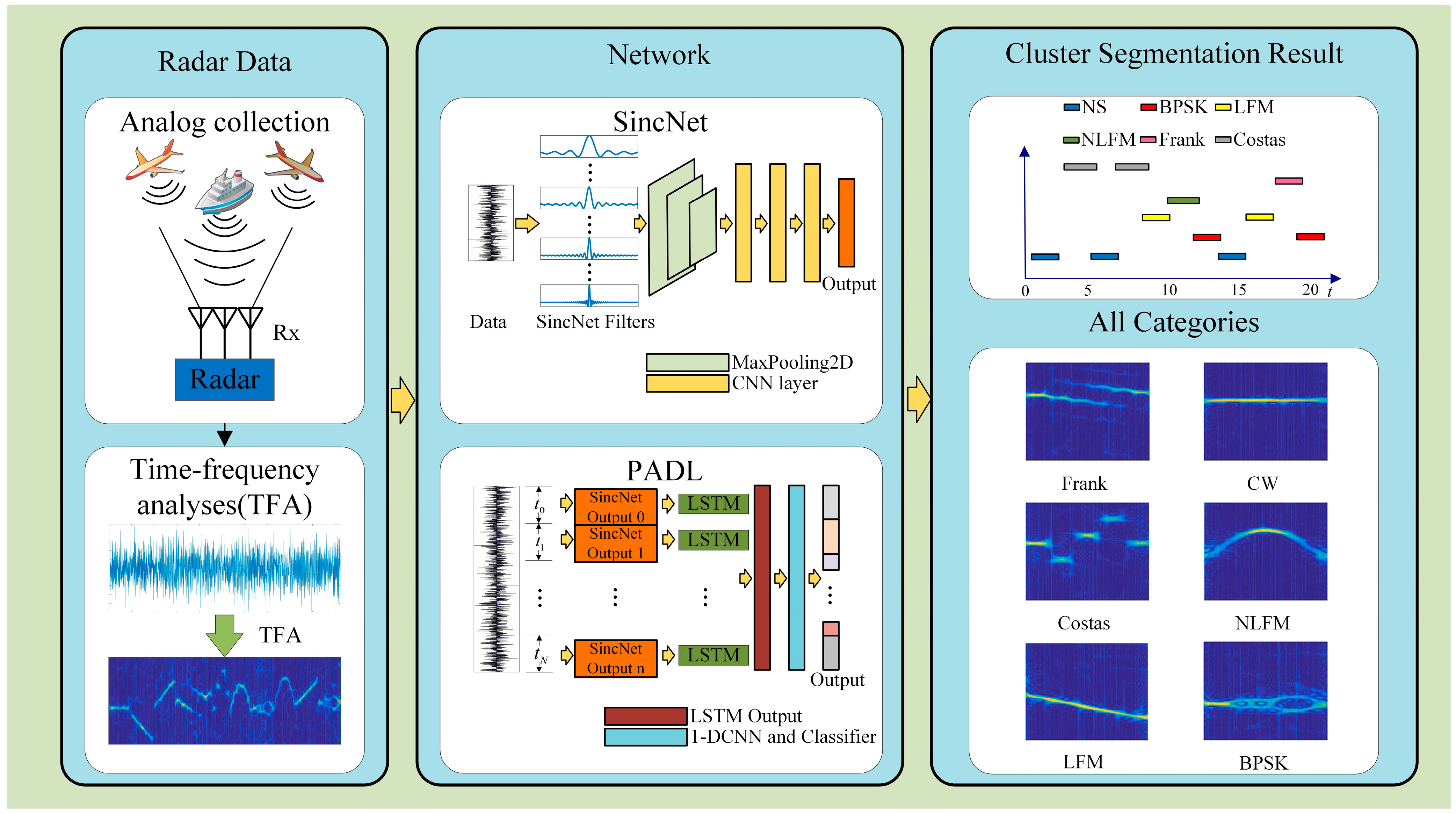
2. Multi-Radar Clustering and Segmentation Networks
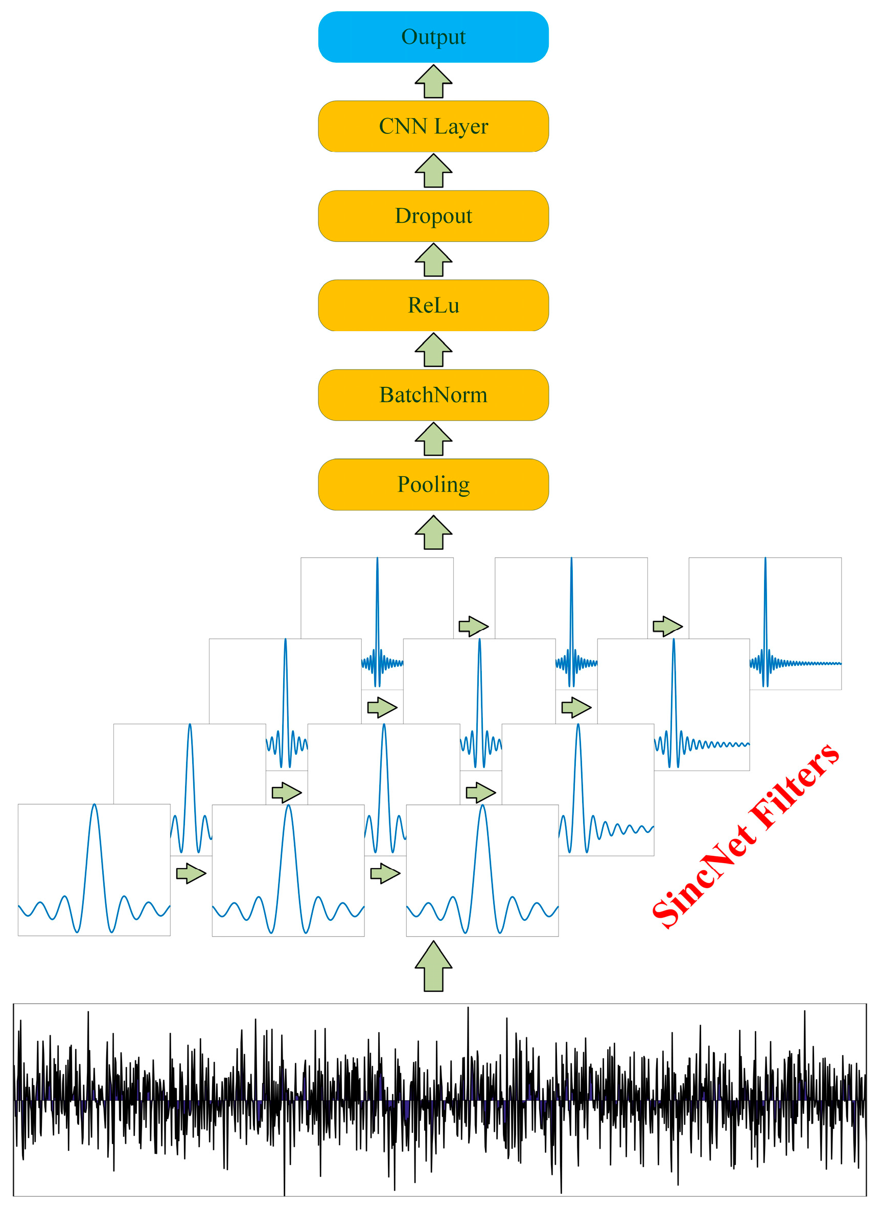
2.1. SincNet Architecture
2.2. Pulse Activity Detection
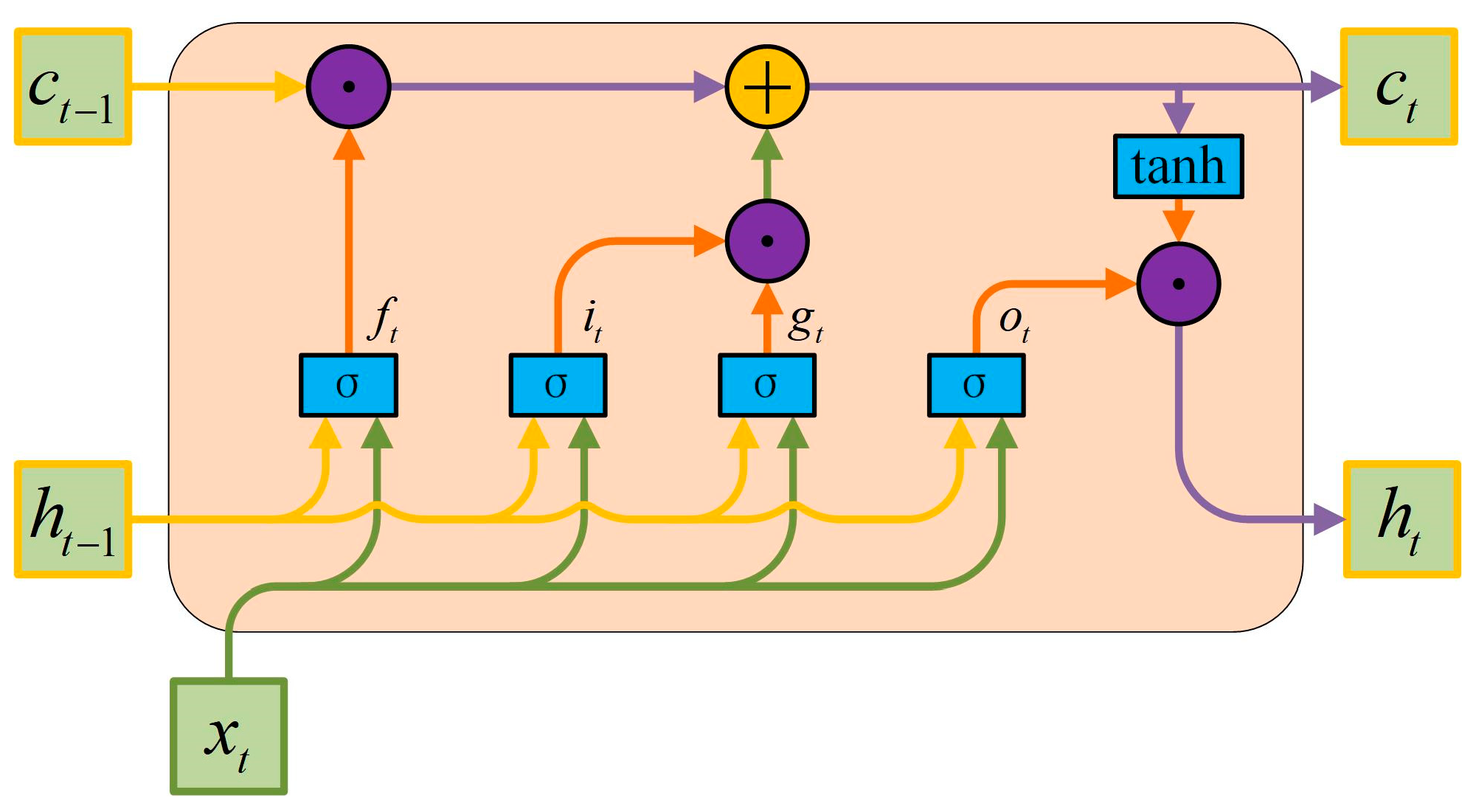
2.2.1. Long Short-Term Memory Network
2.2.2. 1-D Convolutional Neural Network and Classifier
2.2.3. Model Parameter Setting
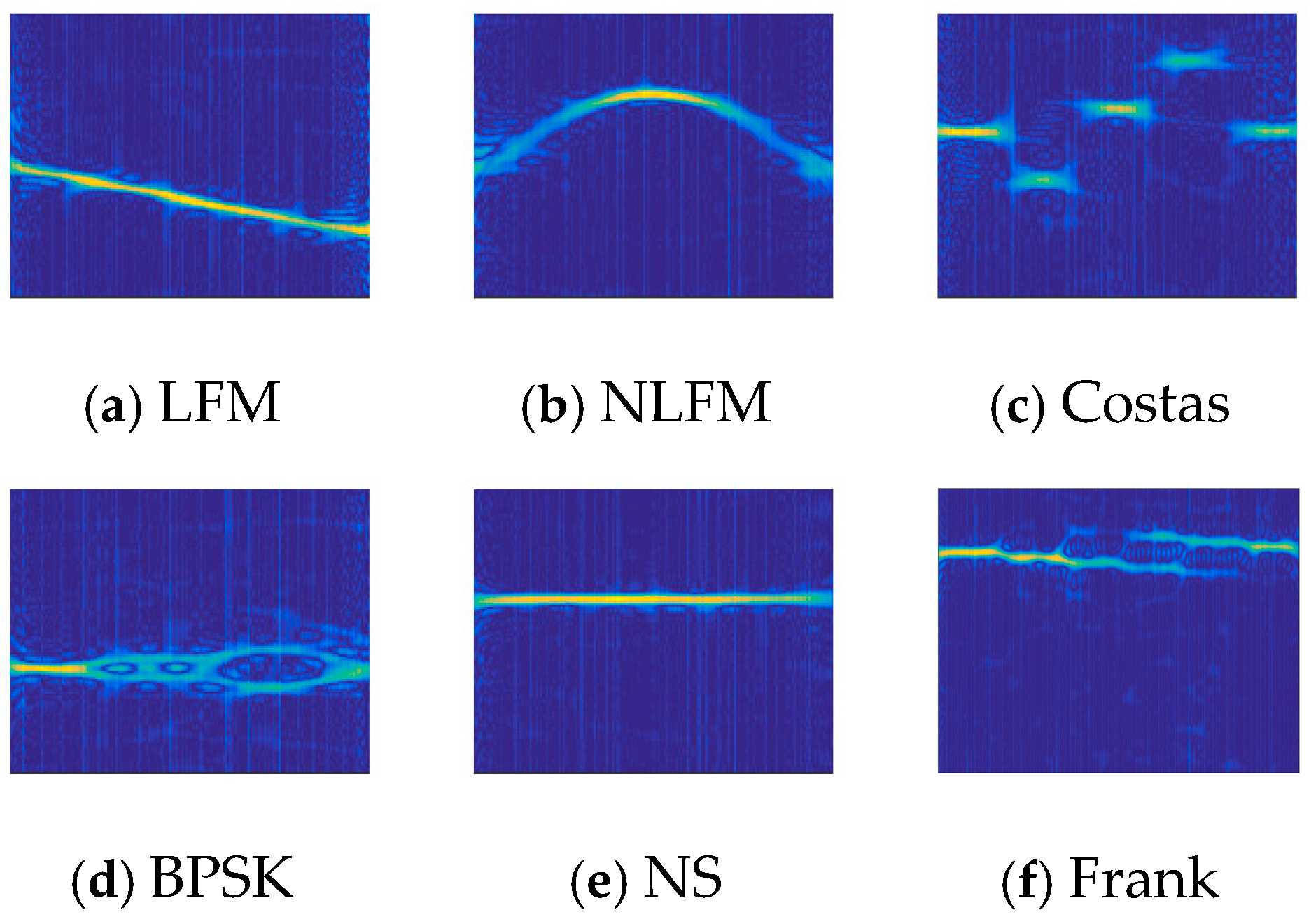
3. Simulation and Time–Frequency Analysis of Radar Signals
3.1. Simulation of Radar Signals
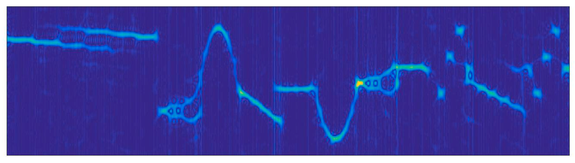
3.2. Time–Frequency Analysis
4. Experimental Results and Analysis
4.1. Training Process
4.2. Influence Analysis of Network Parameters
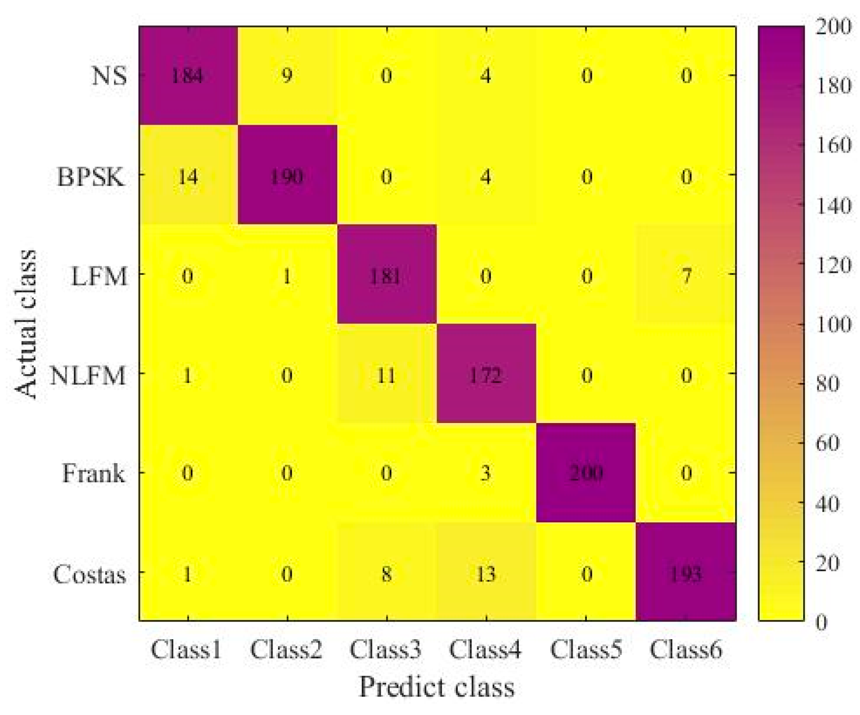
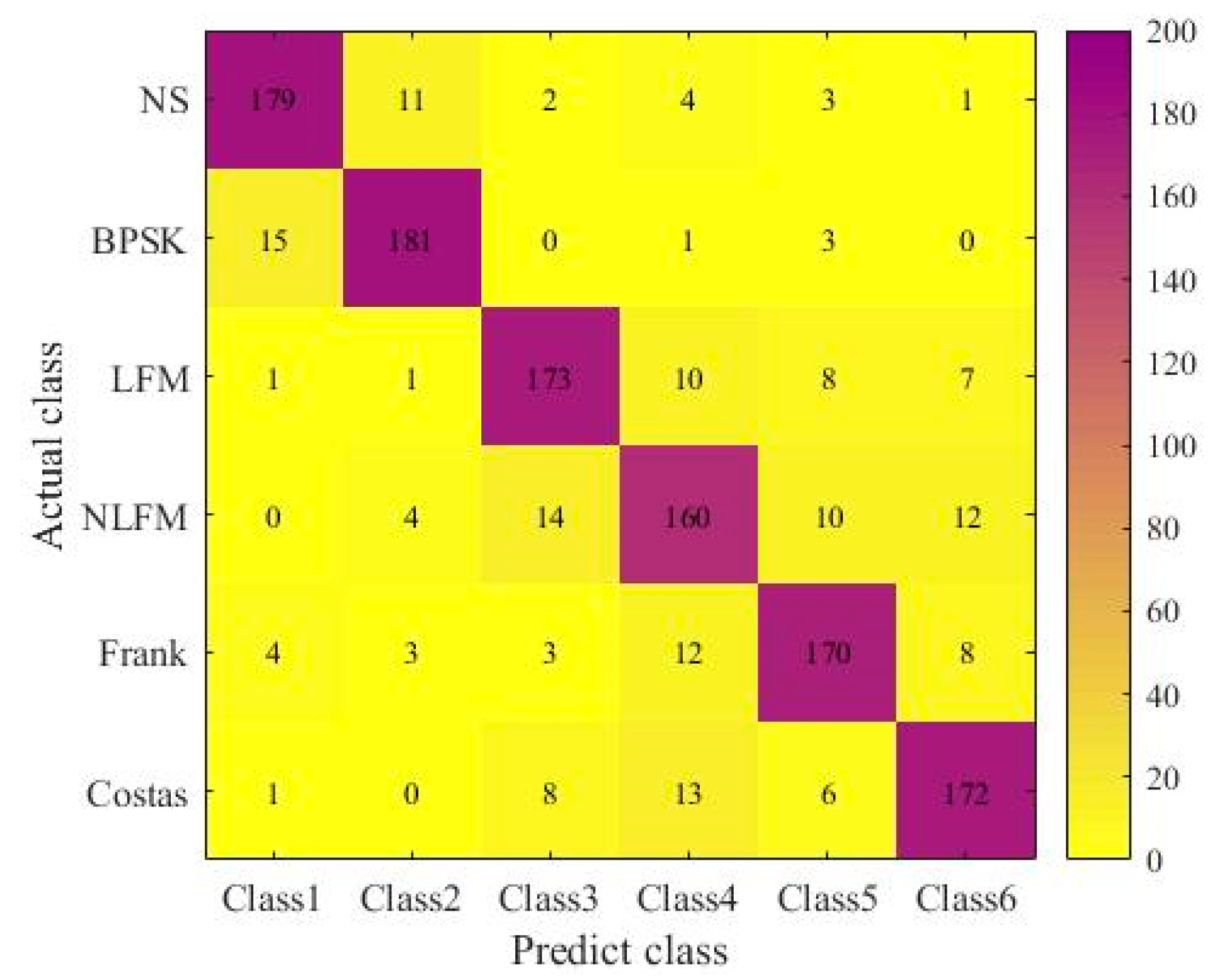
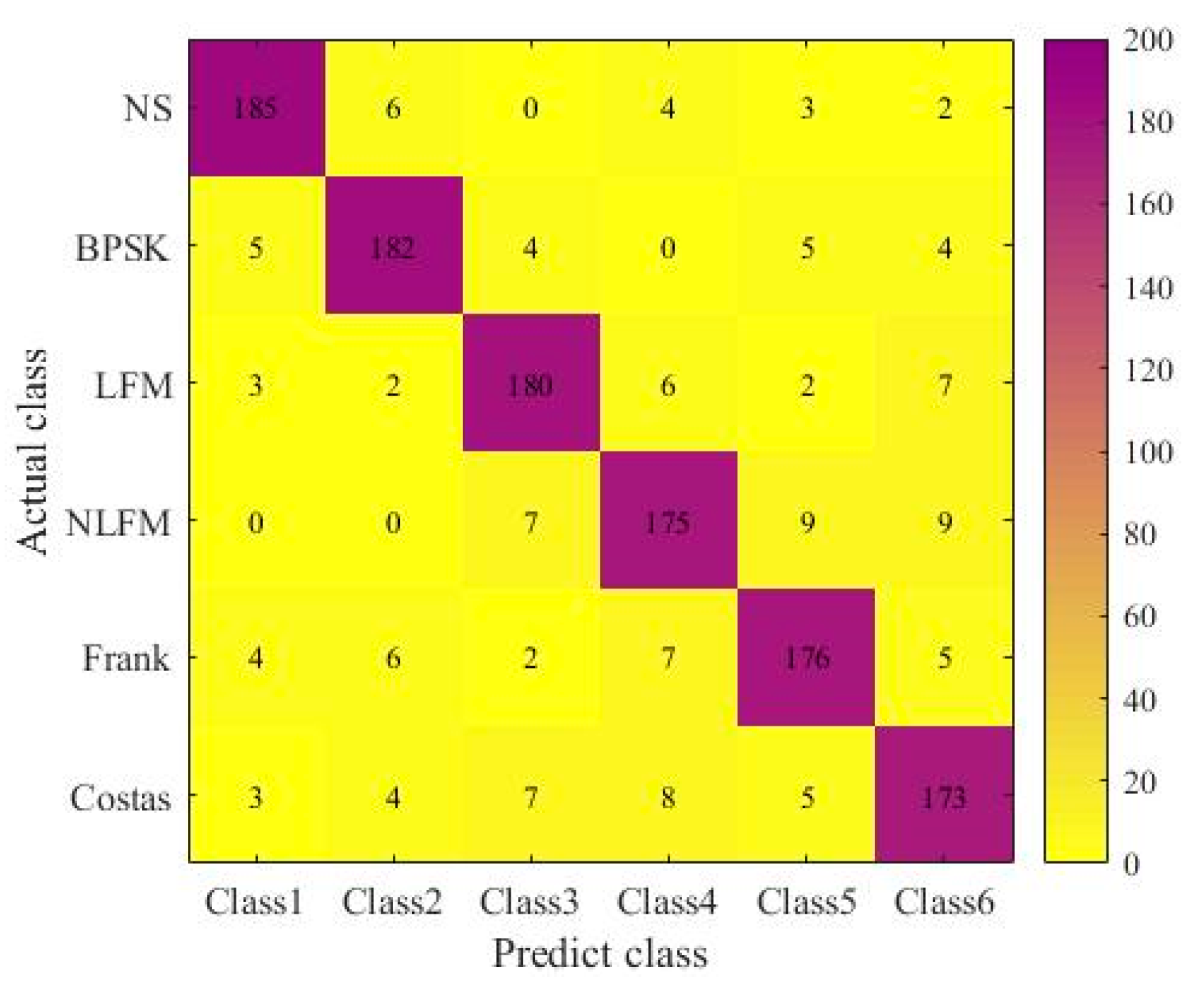
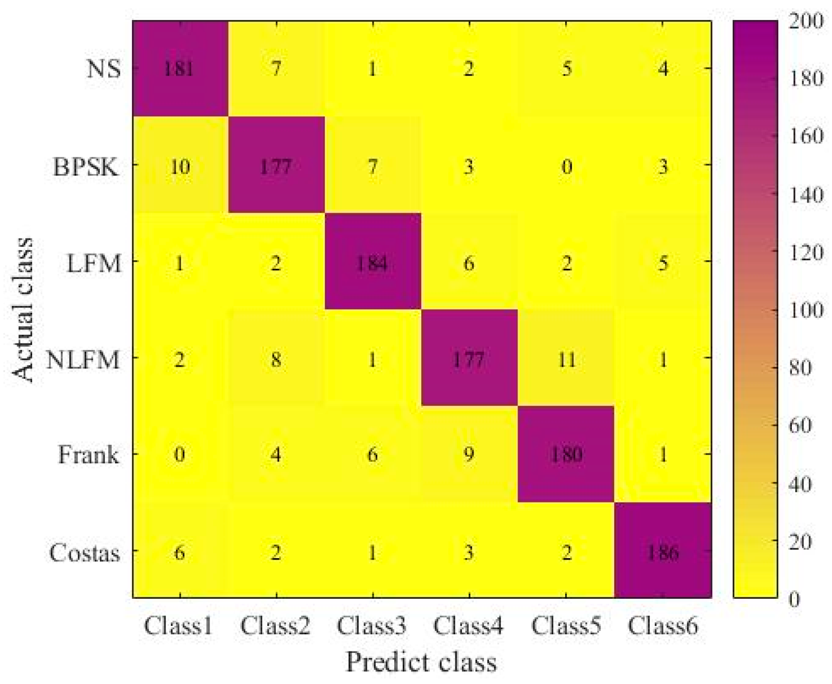
4.3. Experimental Results and Comparative Analysis
5. Conclusions
Author Contributions
Funding
Data Availability Statement
Acknowledgments
Conflicts of Interest
References
- Xu, S.; Ru, H.; Li, D.; Shui, P.; Xue, J. Marine Radar Small Target Classification Based on Block-Whitened TimeFrequency Spectrogram and Pre-Trained CNN. IEEE Trans. Geosci. Remote Sens. 2023, 61, 5101311. [Google Scholar] [CrossRef]
- Wan, H.; Tian, X.; Liang, J.; Shen, X. Sequence-Feature Detection of Small Targets in Sea Clutter Based on Bi-LSTM. IEEE Trans. Geosci. Remote Sens. 2022, 60, 4208811. [Google Scholar] [CrossRef]
- Chen, T.; Liu, Y.; Guo, L.; Lei, Y. A novel deinterleaving method for radar pulse trains using pulse descriptor word dot matrix images and cascade-recurrent loop network. IET Radar Sonar Navig. 2023, 17, 1626–1638. [Google Scholar] [CrossRef]
- Liu, L.; Xu, S. Unsupervised radar signal recognition based on multi-block—Multi-view Low-Rank Sparse Subspace Clustering. IET Radar Sonar Navig. 2022, 16, 542–551. [Google Scholar] [CrossRef]
- Lang, P.; Fu, X.; Cui, Z.; Feng, C.; Chang, J. Subspace Decomposition Based Adaptive Density Peak Clustering for Radar Signals Sorting. IEEE Signal Process. Lett. 2022, 29, 424–428. [Google Scholar] [CrossRef]
- Dong, X.; Liang, Y.; Wang, J. Distributed Clustering Method Based on Spatial Information. IEEE Access 2022, 10, 53143–53152. [Google Scholar] [CrossRef]
- Xu, T.; Yuan, S.; Liu, Z.; Guo, F. Radar Emitter Recognition Based on Parameter Set Clustering and Classification. Remote Sens. 2022, 14, 4468. [Google Scholar] [CrossRef]
- Chen, T.; Yang, B.; Guo, L. Radar Pulse Stream Clustering Based on MaskRCNN Instance Segmentation Network. IEEE Signal Process. Lett. 2023, 30, 1022–1026. [Google Scholar] [CrossRef]
- Mao, Y.; Ren, W.; Li, X.; Yang, Z.; Cao, W. Sep-RefineNet: A Deinterleaving Method for Radar Signals Based on Semantic Segmentation. Appl. Sci. 2023, 13, 2726. [Google Scholar] [CrossRef]
- Prashanth, H.C.; Rao, M.; Eledath, D.; Ramasubramanian, C. Trainable windows for SincNet architecture. Eurasip J. Audio Speech Music. Process. 2023, 2023, 3. [Google Scholar] [CrossRef]
- Wei, G.; Zhang, Y.; Min, H.; Xu, Y. End-to-end speaker identification research based on multi-scale SincNet and CGAN. Neural Comput. Appl. 2023, 35, 22209–22222. [Google Scholar] [CrossRef]
- Yu, Y.; Si, X.; Hu, C.; Zhang, J. A Review of Recurrent Neural Networks: LSTM Cells and Network Architectures. Neural Comput. 2019, 31, 1235–1270. [Google Scholar] [CrossRef] [PubMed]
- Chen, L.; Li, S.; Bai, Q.; Yang, J.; Jiang, S.; Miao, Y. Review of Image Classification Algorithms Based on Convolutional Neural Networks. Remote Sens. 2021, 13, 4712. [Google Scholar] [CrossRef]


| Subnetwork | Network Layer | Hyperparameters | Value | FLOPs |
|---|---|---|---|---|
| SincNet | Sinc filter | Window Function | Hamming | 10.5 M |
| Maxpool | Pooling Size | 1 × 2 | 10.2 K | |
| Dropout | Dropout | 0.5 | 10.2 K | |
| Conv1D | Kenel Size | 1 × 3 | 4.47 M | |
| LSTM | LSTM | Neuron Number | 256 | 34.3 M |
| 1-DCNN | Conv1D | Kenel Size | 1 × 3 | 1.6 M |
| Maxpool | Pooling Size | 1 × 2 | 4.1 K | |
| Conv1D | Kenel Size | 1 × 3 | 1.6 M | |
| Classifier | Full connected layer | Units | 128 | 49.2 K |
| Classifier | Full connected layer | Units | C | 2.3 K |
| Signal Waveforms | Parameters | Uniform Ranges |
|---|---|---|
| LFM&NLFM | Normalized sampling rate | 1 |
| Number of samples | [600, 1200] | |
| Initial frequency | ||
| Coastas | [600, 1200] | |
| Number changed | [3, 6] | |
| BPSK | [600, 1200] | |
| Barker codes | [8] | |
| Carrier frequency | ||
| Frank | [600, 1200] | |
| Frequency steps | [4, 8] | |
| NS | [600, 1200] | |
| Filter Size of 1-DCNN | Number of LSTM Units | Dropout | Accuracy |
|---|---|---|---|
| 1 × 3 | 16 | 0.25 | 92.45% |
| 32 | 93.08% | ||
| 64 | 92.91% | ||
| 1 × 2 | 32 | 90.83% | |
| 1 × 3 | 94.26% | ||
| 1 × 4 | 93.28% | ||
| 1 × 5 | 92.67% | ||
| 1 × 3 | 16 | 0.5 | 95.41% |
| 32 | 96.75% | ||
| 64 | 94.80% | ||
| 1 × 2 | 32 | 92.17% | |
| 1 × 3 | 96.75% | ||
| 1 × 4 | 95.39% | ||
| 1 × 5 | 95.12% | ||
| 1 × 3 | 16 | 0.75 | 91.50% |
| 32 | 92.11% | ||
| 64 | 92.02% | ||
| 1 × 2 | 32 | 87.44% | |
| 1 × 3 | 92.52% | ||
| 1 × 4 | 92.39% | ||
| 1 × 5 | 91.71% |
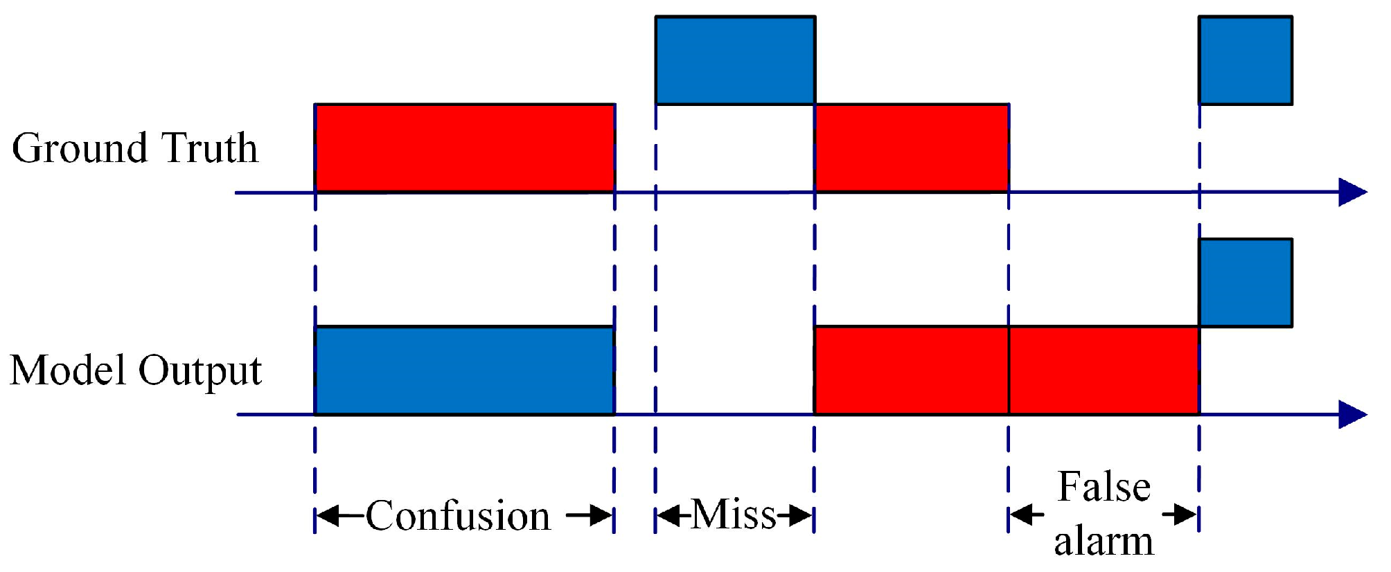
| Network | Confusion | Miss | False alarm | SER |
|---|---|---|---|---|
| MRCS | 4.24% | 4.95% | 0.43% | 9.62% |
| Single 1-DCNN | 4.61% | 4.96% | 0.70% | 10.27% |
| Single LSTM | 4.88% | 5.48% | 1.21% | 11.57% |
| Temporal Overlap Ratio | MRCS | Single 1-DCNN | Single LSTM | ResNet |
|---|---|---|---|---|
| 10% | 96.0% | 93.6% | 91.3% | 94.1% |
| 15% | 92.2% | 89.6% | 85.1% | 90.7% |
| 20% | 87.9% | 82.1% | 76.4% | 86.0% |
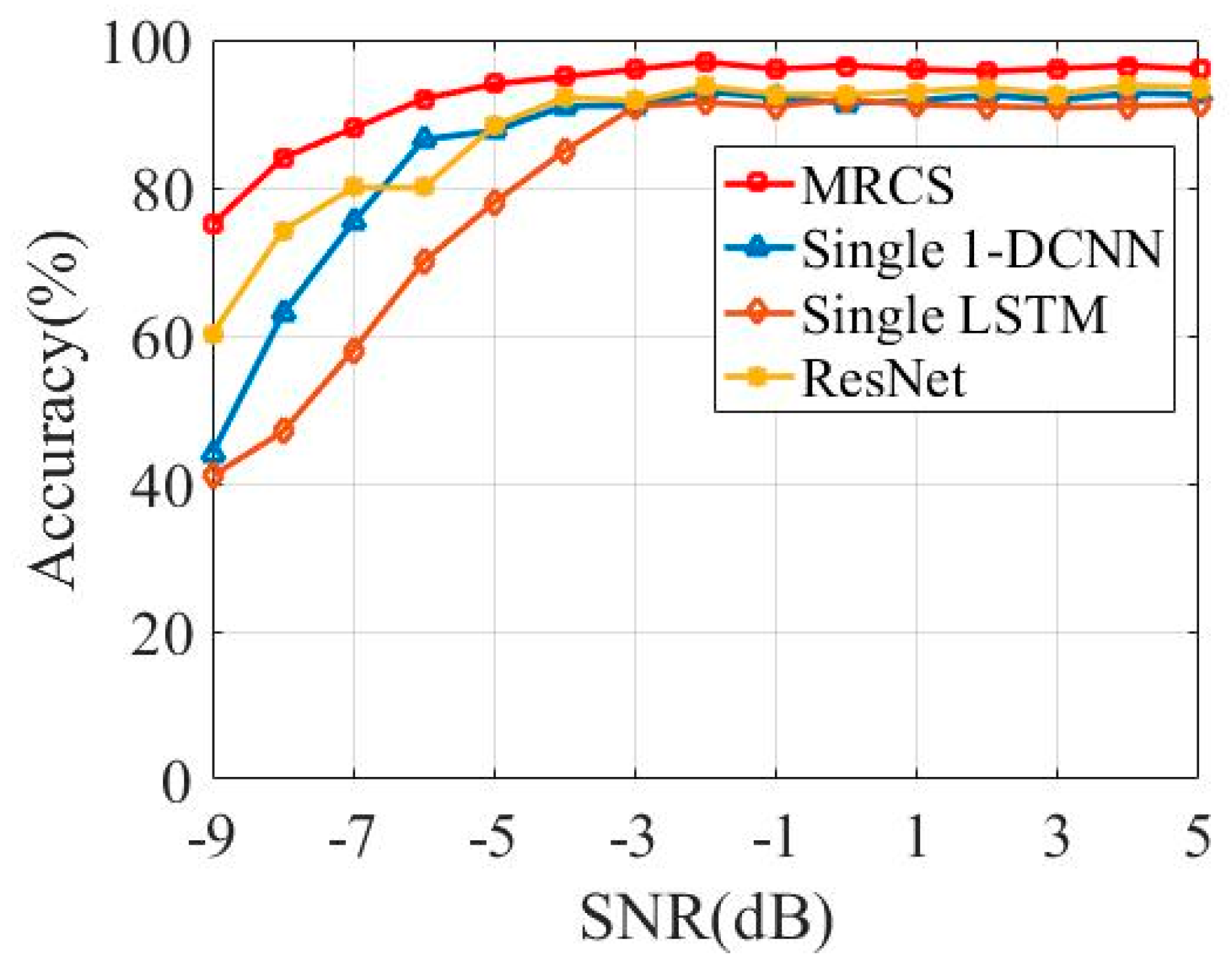
| SNR | MRCS | Single 1-DCNN | Single LSTM | Resnet |
|---|---|---|---|---|
| −9 | 31.5% | 21.3% | 30.7% | 30.4% |
| −7 | 48.2% | 35.1% | 45.5% | 47.1% |
| −5 | 62.6% | 49.8% | 58.1% | 59.0% |
| −3 | 75.7% | 60.2% | 70.8% | 71.9% |
| −1 | 82.0% | 68.7% | 73.2% | 78.9% |
| 1 | 86.7% | 73.4% | 78.7% | 80.5% |
| 3 | 87.5% | 75.1% | 77.0% | 82.6% |
| 5 | 88.3% | 75.3% | 77.6% | 82.7% |
Disclaimer/Publisher’s Note: The statements, opinions and data contained in all publications are solely those of the individual author(s) and contributor(s) and not of MDPI and/or the editor(s). MDPI and/or the editor(s) disclaim responsibility for any injury to people or property resulting from any ideas, methods, instructions or products referred to in the content. |
© 2025 by the authors. Licensee MDPI, Basel, Switzerland. This article is an open access article distributed under the terms and conditions of the Creative Commons Attribution (CC BY) license (https://creativecommons.org/licenses/by/4.0/).
Share and Cite
Chen, T.; Lei, Y.; Guo, L.; Yang, B. MRCS-Net: Multi-Radar Clustering Segmentation Networks for Full-Pulse Sequences. Remote Sens. 2025, 17, 1538. https://doi.org/10.3390/rs17091538
Chen T, Lei Y, Guo L, Yang B. MRCS-Net: Multi-Radar Clustering Segmentation Networks for Full-Pulse Sequences. Remote Sensing. 2025; 17(9):1538. https://doi.org/10.3390/rs17091538
Chicago/Turabian StyleChen, Tao, Yu Lei, Limin Guo, and Boyi Yang. 2025. "MRCS-Net: Multi-Radar Clustering Segmentation Networks for Full-Pulse Sequences" Remote Sensing 17, no. 9: 1538. https://doi.org/10.3390/rs17091538
APA StyleChen, T., Lei, Y., Guo, L., & Yang, B. (2025). MRCS-Net: Multi-Radar Clustering Segmentation Networks for Full-Pulse Sequences. Remote Sensing, 17(9), 1538. https://doi.org/10.3390/rs17091538