Time-Series Modeling of Ozone Concentrations Constrained by Residual Variance in China from 2005 to 2020

Abstract

Satellite retrievals can capture the spatiotemporal variation of O₃ over a large area near the surface. However, due to the unstable functional relationships between variables across spatiotemporal scales, the outlier predictions will reduce the accuracy of the prediction model. Therefore, a validated residual constrained random forest model (RF-RVC) is proposed to estimate the monthly and annual O₃ concentration datasets of 0.1° in China from 2005 to 2020 using O₃ precursor remote-sensing data and other auxiliary data. The temporal and spatial variations of O₃ concentrations in China and the four urban agglomerations (Beijing–Tianjin–Hebei (BTH), Yangtze River Delta (YRD), Pearl River Delta (PRD) and Sichuan–Chongqing (SC)) were calculated. The results show that the annual R² and RMSE of the RF-RVC model are 0.72~0.89 and 8.4~13.06 μg/m³. Among them, the RF-RVC model with the temporal residuals constraint has the greatest performance improvement, with the annual R² increasing from 0.59 to 0.8, and the RMSE decreasing from 17.24 μg/m³ to 10.74 μg/m³, which is significantly better than that of the RF model. The North China Plain is the focus of ozone pollution. Summer is the season of a high incidence of ozone pollution in China, YRD, PYD, and SC, while pollution in the PRD is delayed to October due to the monsoon. In addition, the trend of the O₃ and its excess proportion in China and the four urban agglomerations is not satisfactory; targeted measures should be taken to reduce the risk of environmental ozone. The research findings confirm the effectiveness of the residual constraint approach in long-term time-series modeling. In the future, it can be further extended to the modeling of other pollutants, providing more accurate data support for health risk assessments.

1. Introduction

As a typical secondary pollutant, near-surface O₃ is mainly generated by the photochemical reaction of precursors, such as volatile organic compounds (VOCs) and nitrogen oxides (NOx), under the action of solar ultraviolet light [1]. Although near-surface O₃ accounts for about 10% of the O₃ content of the entire atmosphere, its impact on ecosystems and human health cannot be ignored [2,3,4]. Since 2013, China has launched the Action Plan for Prevention and Control of Air Pollution (APPCAP), which has effectively curbed PM_2.5 pollution; however, O₃ concentrations have shown a rapid increase and a spreading trend. Between 2013 and 2019, annual O₃ concentrations in China increased by 28.8%; about 26.24% of the population was exposed to O₃ concentrations exceeding 160 μg/m³ [5,6]. In 2020, 16.6% of Chinese cities had annual O₃ concentrations exceeding the national secondary standard [6]. By 2022, China accumulated 1734 air-quality monitoring stations nationwide, providing effective support for air pollution control in China [7]. However, the limited number of monitoring stations cannot provide full coverage of high-precision spatial distribution information about surface O₃ and are insufficient to support the growing demands of environmental management in China [8,9]. At the same time, monitoring stations are primarily concentrated in the eastern regions of China and urban centers, resulting in insufficient air-quality monitoring coverage in the western regions and vast rural areas of the country [10,11]. On the other hand, due to the fact that the construction of the air-quality monitoring network in China started in 2013, there is no way to know the real-time air-quality situation before 2013. The lack of historical O₃ concentration observations makes it challenging to estimate the distribution of near-surface O₃ concentrations before 2013 [5].

Satellite monitoring makes it possible to map O₃ concentrations over a wide range. Previous studies have shown that remote-sensing data of precursor pollutants and meteorological data can effectively explain the spatial and temporal variation of O₃ concentrations at the site, and can be successfully extended to the entire spatial range [1,12,13]. At present, the main methods used to interpret the relationship between station O₃ concentrations and remote-sensing data can be divided into chemical transport models (CTMs), statistical regression models, and machine learning models [14]. The chemical transport model, grounded in physical principles, simulates concentrations by taking into account atmospheric chemical reactions, meteorological conditions, and emissions inventories. It is suitable for estimating concentrations over a large area and is interpretable [15]. Statistical regression models achieve predictive simulations by calculating the regression relationship between O₃ concentrations and precursors and meteorological conditions, with good accuracy results. For example, multiple linear regression (MLR) [16], land-use regression (LUR) [17,18,19], geographically weighted regression (GWR) [20,21] etc., are used. However, the complex relationships among different variables hinder further improvements in their accuracy [14]. Machine learning has advantages in processing massive data and non-linear relationships between variables; therefore, it is increasingly popular among researchers. These include models such as random forest (RF) [22,23], deep forest (DF) [6], light gradient boosting machine (LightGBM) [24,25], space–time extremely randomized trees (STET) [26], and Geo-STO₃Net [27], etc.

The idea of O₃ modeling, in existing studies, is usually to construct a statistical relationship model between the measured O₃ concentrations and various variables, and then to obtain the O₃ concentrations at different times and spaces through the constructed model and various variables. The functional relationship of different variables is usually stable in the short term, but in the case of a long-time span, there are still challenges to maintain the stability of the functional relationship [28,29]. One possible scenario under this modeling approach is that the modeled relationship at one time and space may not be applicable to another time and space [30,31]. For example, if the model is constructed by dividing regions or dividing years while the model structure and modeling variables remain the same, some years or regions will have high accuracy and some will have low accuracy [32]. Previous studies have shown that such high error results are mainly due to the fact that static models based on short time-series samples cannot effectively construct the spatial and temporal change relationships between long time-series variables; the outliers caused by abnormal functional relationships increase the uncertainty of static models [32]. Therefore, it is feasible to improve model reliability by eliminating the outliers in the modeling samples [29,33].

Based on the idea of residual correction, we exclude model outliers to obtain more reliable results. The framework of this study is as follows: (1) an O₃ modeling accuracy correction method (RF-RVC) is constructed based on the residual correction idea; (2) a cross-validation (CV) comparison of modeling accuracy before and after residual correction is conducted; and (3) RF-RVC is used to reconstruct near-surface O₃ concentrations in China and analyze the four time-series indicators.

2. Data and Methods

2.1. Data

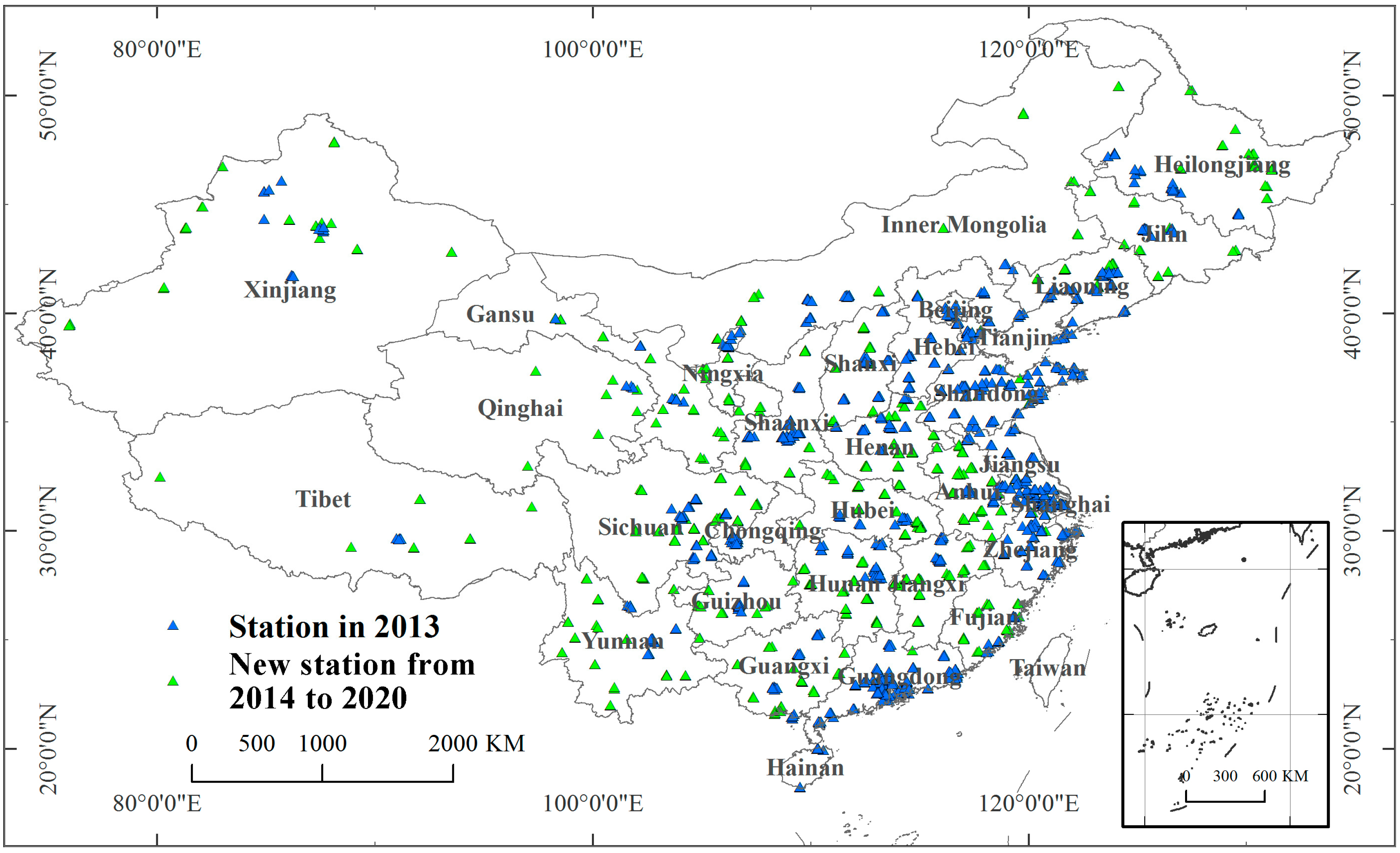
2.1.1. Ground Monitoring Data

Air-quality monitoring stations have been constructed on a large scale in China since 2013. Hourly O₃ concentration (µg/m³) monitoring data from ground stations for the period 2013 to 2020 were obtained from the China National Environmental Monitoring Center (www.cnemc.cn (accessed on 4 Augst 2024)). These data were taken at an atmospheric temperature of 298.15 K and an atmospheric pressure of 1013.25 hPa. Any invalid values were rejected [34]. The spatial distribution of the stations in 2013 and new stations from 2014 to 2020 are shown in Figure 1.

In accordance with the relevant specifications of the national “Ambient Air Quality Standards” (GB3095-2012), quality control was conducted on the collected O₃ ground station concentration data. The specific process is as follows: (1) eliminate records with missing hourly concentrations or negative values in the raw data; (2) eliminate records with fewer than 20 data points within 24 h of a natural day and calculate daily maximum 8-h mean value (MDA8); (3) eliminate stations with fewer than 27 daily mean concentration values per month (at least 25 daily mean concentration values in February) and calculate the 90th percentile of the daily maximum value (O₃_MDA8_90) as the monthly O₃ concentration value; and (4) eliminate stations with fewer than 324 daily mean concentration values per year and calculate the MDA8_90 as the annual O₃ concentration value.

2.1.2. NO₂ Tropospheric Vertical Column Density Data

The NO₂ tropospheric vertical column density (TVCD) data were sourced from the NASA GES DISC database website (https://disc.gsfc.nasa.gov/ (accessed on 4 Augst 2024)), with a spatial resolution of 24 × 13 km and a temporal resolution of days. In this study, we selected the OMI-NO₂ column concentration data product from the AURA satellite, covering the time period from 2005 to 2020 [35]. We resampled the data to 0.1° and aggregated all daily data for each month to calculate the monthly mean value, which was calculated only when each grid had values for at least 20 days of the month. The annual mean value was obtained from the arithmetic mean of the monthly mean value.

2.1.3. HCHO Column Concentration Data

HCHO is another major precursor pollutant for near-surface O₃ pollution [36]. Since the same sensor is usually used to detect HCHO and NO₂, a detailed description of HCHO data is not provided here. The acquisition method and data preprocessing process of HCHO data are consistent with those of NO₂.

2.1.4. Meteorological Data

The meteorological data were sourced from the ERA5-LAND reanalysis dataset provided by the European Centre for Medium-Range Weather Forecasts (ECWMF) (https://cds.climate.copernicus.eu/ (accessed on 4 Augst 2024)). This article selected atmospheric boundary layer height, temperature, pressure, wind speed, wind direction, relative humidity, rainfall, and surface solar radiation as meteorological factors. Air temperature and surface solar radiation directly affect the rate of O₃ photochemical reactions; high temperatures and strong solar radiation are important factors causing high O₃ pollution [20,37]. Wind direction and wind speed can affect the accumulation and diffusion of O₃; air pressure and precipitation can also indirectly affect the O₃ concentration in the lower troposphere [6,38,39,40]. ERA5-LAND utilizes the land surface atmospheric variables simulated by the ECWMF’s fifth-generation reanalysis product ERA5 as forcing; these were obtained through simulations using the modified land surface hydrological models HTESSEL and CY45R1. Compared to ERA5, ERA5-LAND boasts a higher spatial resolution, with a spatial resolution of 0.1° × 0.1°. The original dataset provides hourly and monthly mean data. For this article, data from 2005 to 2020 were selected; annual mean meteorological data were obtained by calculating the arithmetic mean of the monthly mean data.

2.1.5. WorldPop Data

Annual gridded population data (1 × 1 km, 2005–2020) from the WordPop dataset (https://www.worldpop.org/ (accessed on 4 Augst 2024)) were used. The total population of the dataset was estimated by integrating census data, remote-sensing data, building area data and other multi-source data, using top–down and bottom–up methods [41].

2.1.6. Other Auxiliary Data

The surface data proposed in this study encompass the Enhanced Vegetation Index (EVI) [42], topographic elevation data [5], and nighttime light data products [43]. The EVI was sourced from the LAADS DAAC (https://ladsweb.modaps.eosdis.nasa.gov/ (accessed on 4 Augst 2024)) website, and the data product is the EVI retrieved by the MODIS Terra/Aqua satellite, with product codes MOD13A2/MYD13A2. Its spatial resolution is 1 km, and the temporal resolution is 16 days. The preprocessing procedures for MODIS EVI data, such as stitching, cropping, and projection, can be handled by the LAADS DAAC website back end. Vegetation can affect the generation and diffusion of ozone; therefore, EVI was selected to represent the density of the vegetation distribution in space. The topographic elevation data were used to characterize the surface topography and geomorphology, which affect the propagation and diffusion of ozone. Data were sourced from NASA’s SRTM data (https://srtm.csi.cgiar.org/ (accessed on 4 Augst 2024)). The spatial resolution is 90 m × 90 m. The nighttime light data utilize the long-term (2005~2020) annual-scale nighttime light remote-sensing data product published by Chen et al. [44]. (https://doi.org/10.7910/DVN/YGIVCD (accessed on 4 Augst 2024)). The product has a spatial resolution of 500 m × 500 m, with the consistency of R² reaching 0.87 and 0.95 at the pixel level and city level, respectively [44]. Nighttime light remote-sensing data at night can characterize human activities to some extent, while ozone premise pollutants are significantly affected by human activities. All data were resampled and unified to 0.1°.

2.2. Method

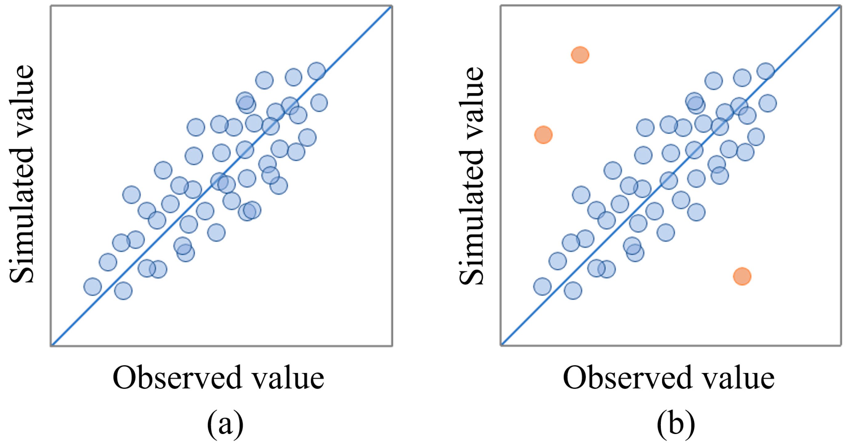
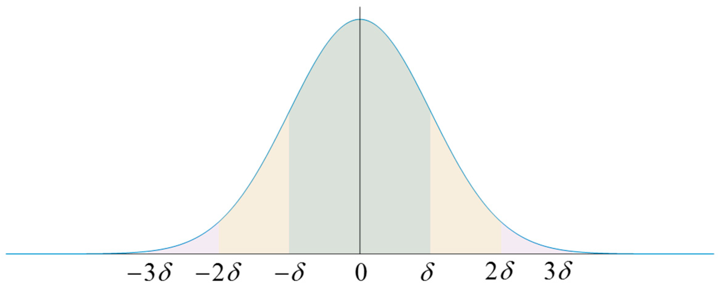
2.2.1. The Concept of Residual Constraint Theory

The accuracy of atmospheric pollution concentration modeling is highly influenced by the modeling sample. In long-term, large-scale modeling processes, theoretically, the model trained by sample data can represent the generalizable patterns of the relationship between pollutant concentrations and various variables. However, when the modeling period is longer and the spatial range is wider, it is difficult for the global model to learn the universal laws of all sample data and some abnormal samples will affect the learning of these universal laws and reduce the accuracy of the model (Figure 2).

The sample error of the model can be obtained from Equation (1):

$$Resi=Obs-Val$$

(1)

where Resi is the model sample error, Val is the model simulated value, and Obs is the sample observed value (O₃_MDA8_90).

Then, the standard deviation of the sample error can be calculated from Equation (2):

$$\delta =\sqrt{{\displaystyle \frac{\sum {\left(Resi-\overline{Resi}\right)}^2}{n}}}=\sqrt{{\displaystyle \frac{\sum {\left(Resi-\left(\sqrt{\frac{Resi}{n}}\right)\right)}^2}{n}}}$$

(2)

Assuming that the error of the model follows a Gaussian normal distribution, the probability density curve is shown in Figure 3.

Then, the probability that the model sample error falls into one, two, and three times the standard deviation can be calculated by Equations (3), (4) and (5), respectively [45], as follows:

$${\int }_{-\delta }^{\delta }{\displaystyle \frac{1}{\sqrt{2\pi }\delta }}\exp (-{\displaystyle \frac{Resi}{2{\delta }^2}})d\left(Resi\right)=0.6826$$

(3)

$${\int }_{-2\delta }^{2\delta }{\displaystyle \frac{1}{\sqrt{2\pi }\delta }}\exp (-{\displaystyle \frac{Resi}{2{\delta }^2}})d\left(Resi\right)=0.9545$$

(4)

$${\int }_{-3\delta }^{3\delta }{\displaystyle \frac{1}{\sqrt{2\pi }\delta }}\exp (-{\displaystyle \frac{Resi}{2{\delta }^2}})d\left(Resi\right)=0.997$$

(5)

Therefore, the theoretical probabilities of model sample errors falling within one, two, and three times the standard deviation are 68.26%, 95.45%, and 99.70%, respectively. The probability of samples falling within two times the standard deviation is nearly identical to that within three times the standard deviation. However, the condition of two times the standard deviation is stricter, suggesting that samples outside two times the standard deviation could be excluded in order to retain those with more generalizable patterns for secondary modeling.

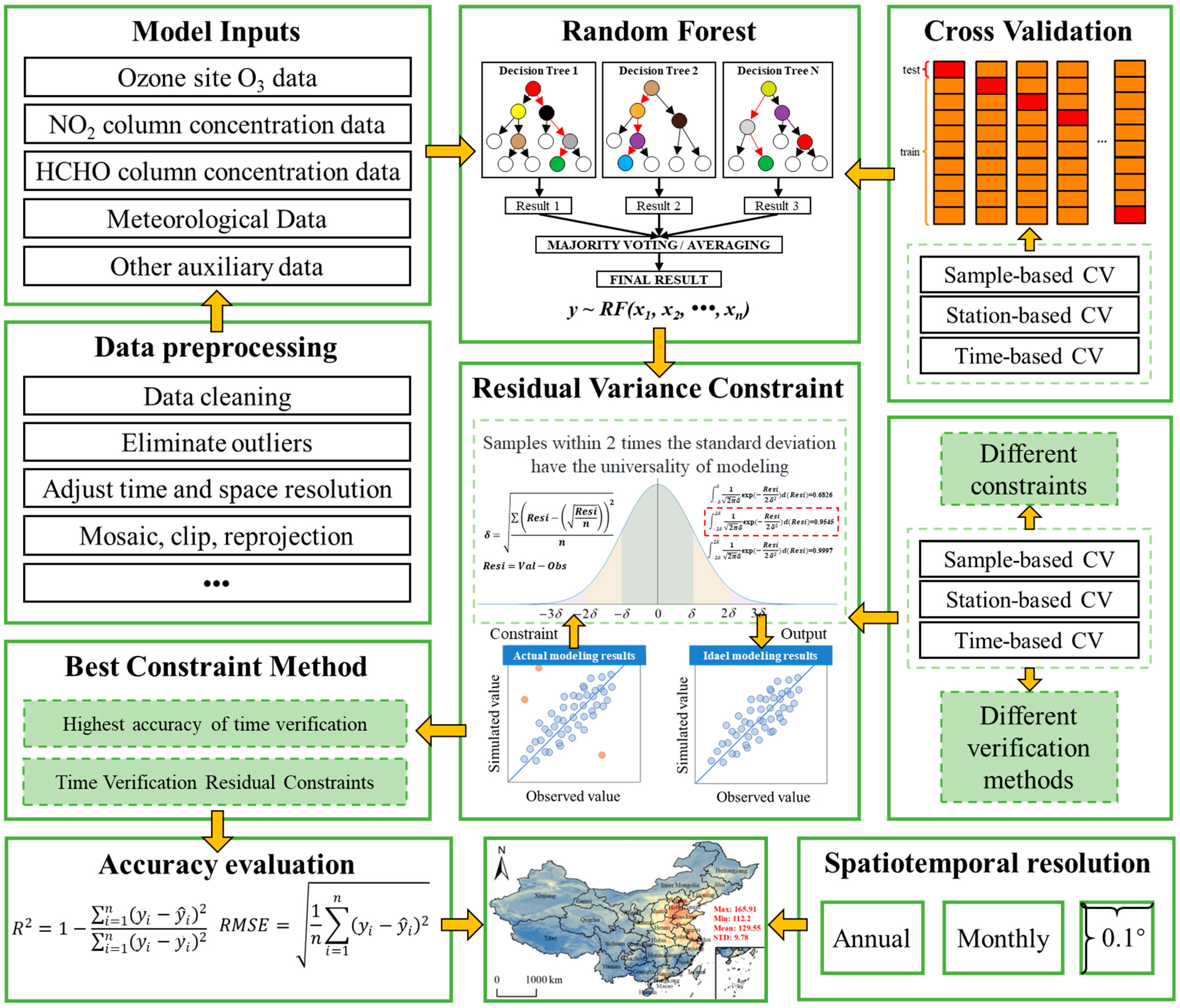
2.2.2. Construction of RF-RVC Model

RF is a statistical learning theory proposed by Breiman [46]. Its essence is to simulate multiple nonlinear relationships by integrating multiple decision trees; it has been widely used in the field of remote-sensing estimation of air pollution concentrations [20,47,48]. The main steps of the RF regression model are divided into three parts: (1) random sampling of sample data and generation of the training set; (2) random selection of feature variables and construction of regression trees; and (3) combining the regression trees generated in the previous step to form the RF regression model, which ultimately obtains the predicted values by taking the mean value.

The sample validation residual constraint random forest model (RF-RVC) is an improved model based on the random forest model, which eliminates abnormal samples through residual constraint to improve accuracy. On the one hand, data-driven statistical models are sensitive to outliers, resulting in large errors. On the other hand, the outlier data will affect the universality of the long time-series model in learning all the sample data, thus reducing the accuracy of the model.

RF-RVC consists of three steps. In the first step, a prediction model is constructed based on a random forest model and performs CV prediction, as shown in Equation (6):

$${\mathrm{O}}_3=RF(x_1,x_2,\cdots x_n)$$

(6)

where O₃ is the ground measured value and x₁~x_n is the predictor.

Step 2: calculate the absolute prediction error (Resi) and standard deviation between the measured value and the predicted result of Step 1, as shown in Equations (1) and (2):

Step 3: the samples constrained by absolute prediction error and standard deviation (within twice the variance) are selected as new datasets and are brought into the random forest model again for CV prediction, as follows:

$${{\mathrm{O}}^{\prime }}_{3(i,j,t)}\in \left\{{\mathrm{O}}_{3(i,j,t)}\left(Resi<2\sigma \right)\right\}$$

(7)

2.2.3. RF-RVC Model Verification

In this study, the data were divided into 10 categories according to samples, stations and times; the 10-fold CV method was used to verify the estimated ozone concentrations. The determination coefficient (R²) and root mean square error (RMSE) were calculated according to the prediction results of the model to test the accuracy of the model. The calculation formula is as follows:

$$R^2=1-{\displaystyle \frac{{\sum }_{i=1}^n{\left(y_i-{\widehat{y}}_i\right)}^2}{{\sum }_{i=1}^n{\left(y_i-{\bar{y}}_i\right)}^2}}$$

(8)

$$RMSE=\sqrt{{\displaystyle \frac{1}{n}}{\sum }_{i=1}^n{\left(y_i-{\widehat{y}}_i\right)}^2}$$

(9)

where y_i is the observed value, ${\bar{y}}_i$ is mean value of observations, and ŷ_i is the predicted value of the model.

Based on the introduction of the above principles and methodology, the specific flow of RF-RVC can be realized by Figure 4.

2.2.4. Ozone Exposure Evaluation Index

In this study, the mean concentration (MC), population-weighted concentration (PWC), proportion of areas with exceeded concentrations (PAE), and the proportion of populations with exceeded concentrations (PPE) were compared and analyzed. The calculation formulas are as follows:

$$M{C}_n={\displaystyle \frac{{\sum }_{n=1}^N{C}_{i,j}}{N}}$$

(10)

where MC_n is the mean concentration of region n, N is the number of concentration grids in region n, and C_i,j is the concentration value of the (i, j)th grid in region n, as follows:

$$PW{C}_n={\displaystyle \frac{{\sum }_{n=1}^N{C}_{i,j}\times P_{i,j}}{{\sum }_{n=1}^N{P}_{i,j}}}$$

(11)

where PWC_n is the population-weighted concentration of region n, N is the number of concentration grids within region n, C_i,j is the concentration value of the (i, j)th grid in region n, and P_i,j is the population of the (i, j)th grid in region n, as follow:

$${PAE}_n={\displaystyle \frac{Area\left(m\right)}{Area\left(n\right)}}\times 100\mathrm{\%},m=\left\{C_{i,j}\ge C_{LT}\right\}$$

(12)

where PAE_n is the excess area ratio of region n, Area(n) denotes the total area of region n, m is the aggregate area of the concentration excess grid in region n, Area(m) is the area of region m, C_i,j is the (i, j)th grid concentration value in region n, and C_LT stands for the concentration standard value, as follows:

$${PPE}_n={\displaystyle \frac{{\sum }_{m=1}^M{P}_{m,n}}{{\sum }_{n=1}^N{P}_{i,j}}}\times 100\mathrm{\%},m=\left\{C_{i,j}\ge C_{LT}\right\}$$

(13)

where PPE_n is the population ratio of region n living under the concentration exceeding the standard, N is the number of grids in region n, P_i,j signifies the population of the (i, j)th grid in region n, m is the set area of the concentration exceeding the standard grid in region n, M is the number of grids in region m, P_m,n is the population of the (m, n)th grid in region m, C_i,j is the (i, j)th grid concentration value in region n, and C_LT is the concentration standard value.

In the calculation process of PAE and PPE, the standard value for O₃ concentrations was derived from the Ambient Air Quality Standards (GB 3095-2012). The annual primary standard (LT-1) for O₃ concentration was set at 100 µg/m³, and the secondary standard (LT-2) was set at 160 µg/m³. Since the monthly concentration limit is not given in the standard (GB 3095-2012), the daily primary standard (100 µg/m³) and secondary standard (160 µg/m³) were taken as the concentration limit standards for the monthly scale in this study.

3. Results

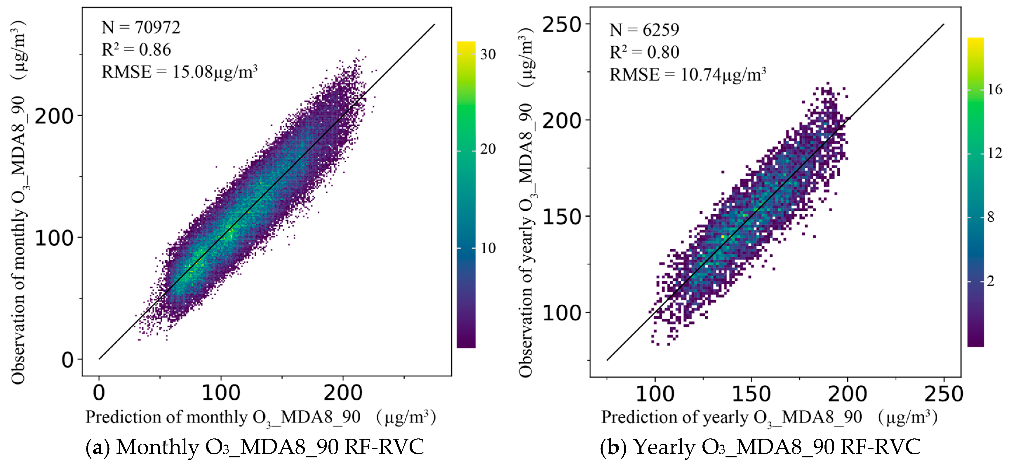
3.1. Evaluation of Model Accuracy

Comparison of Accuracy Between RF-RVC and RF-WRVC

Table 1. Comparison of model accuracy before residual constraints and using different constraint methods.

Time Scale	Restraint Mode	Number of Samples	R2			RMSE (µg/m3)
			Sample-Based	Station-Based	Time-Based	Sample-Based	Station-Based	Time-Based
Monthly scale	Absence of restriction	82,453	0.83	0.82	0.69	18.50	18.93	24.70
	Sample validation residuals	73,156	0.92	0.91	0.82	12.07	12.30	17.92
	Station verification residuals	73,070	0.92	0.92	0.82	12.08	12.21	18.00
	Time verification residuals	70,972	0.91	0.90	0.86	12.31	12.67	15.08
Annual scale	Absence of restriction	7232	0.79	0.77	0.59	12.35	12.95	17.24
	Sample validation residuals	6357	0.89	0.87	0.73	8.40	8.82	12.91
	Station verification residuals	6335	0.88	0.88	0.72	8.51	8.63	13.06
	Time verification residuals	6259	0.87	0.85	0.80	8.76	9.36	10.74

shows the comparison of model accuracy before residual constraints and different constraint methods. In terms of the number of samples, the number of monthly O₃_MDA8_90 modeling samples is 82,453, and the numbers of samples after the residual constraint of sample, station and time validation are 73,156, 73,156 and 70,972, respectively; the actual loss rates of the samples are 11.28%, 11.28% and 13.92%, respectively. The annual O₃_MDA8_90 modeling samples is 7232, and the numbers of samples are 6357, 6335 and 6259 after the residual constraint of sample, station, and time verification; the actual loss rates of the samples are 12.10%, 12.40% and 13.45%, respectively. This result is consistent with our previous study [32].

Evaluation indicators R² and RMSE were used to compare the accuracy of the two models. The results indicated that the residual variance constraint methods validated with samples, station, and times all improve model accuracy. On a monthly scale, after sample, site, and time validated residual constraints, the model R² (RMSE) based on sample validation increased (decreased) from 0.83 (18.50 µg/m³) to 0.92 (12.07 µg/m³), 0.92 (12.08 µg/m³) and 0.91 (12.31 µg/m³), respectively; the model R² (RMSE) based on site validation increased (decreased) from 0.82 (18.93 µg/m³) to 0.91 (12.30 µg/m³), 0.92 (12.21 µg/m³), and 0.90 (12.61 µg/m³), respectively; The model R² (RMSE) based on time validation increased (decreased) from 0.69 (24.70 µg/m³) to 0.82 (17.92 µg/m³), 0.82 (18.00 µg/m³), and 0.86 (15.08 µg/m³), respectively. On the annual scale, after sample, site, and time validated residual constraints, the model R² (RMSE) based on sample validation increased (decreased) from 0.79 (12.35 μg/m³) to 0.89 (8.40 µg/m³), 0.88 (8.51 µg/m³) and 0.87 (8.76 µg/m³), respectively. The model R² (RMSE) based on site validation increased (decreased) from 0.77 (12.95 µg/m³) to 0.87 (8.82 µg/m³), 0.88 (8.63 µg/m³) and 0.85 (9.36 µg/m³), respectively. The model R² (RMSE) based on time validation increased (decreased) from 0.59 (17.24 µg/m³) to 0.73 (12.91 µg/m³), 0.72 (13.06 µg/m³) and 0.80 (10.74 µg/m³), respectively.

The above results show that the RF-RVC model is more stable than the RF model without the residual variance constraint (RF-WRVC) in the time series; therefore, it is more suitable for the construction of long time-series models. Among the three different constraint methods, there is little difference between the accuracy of sample-based and station validation, while the accuracy of the time residual constraint method based on time validation is the most obvious. Therefore, the RF-RVC model based on time validation and time residual constraint is used to map the long time series of O₃ concentrations from 2000 to 2020. The final selected model checking accuracy is shown in Figure 5.

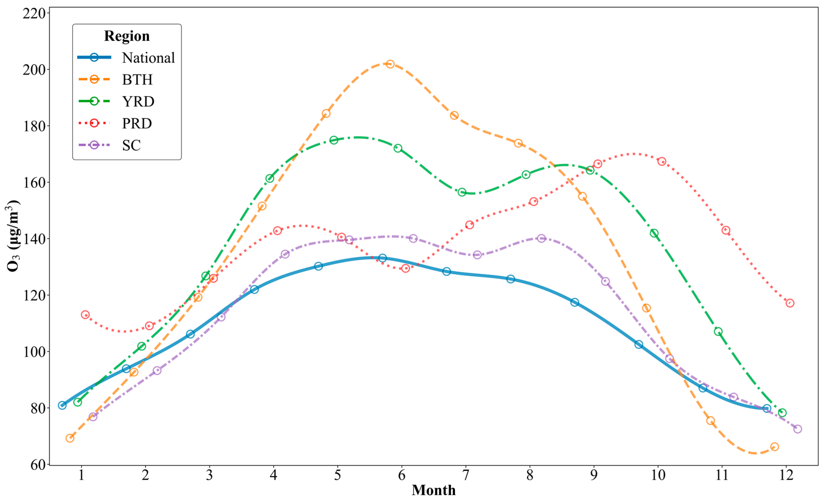
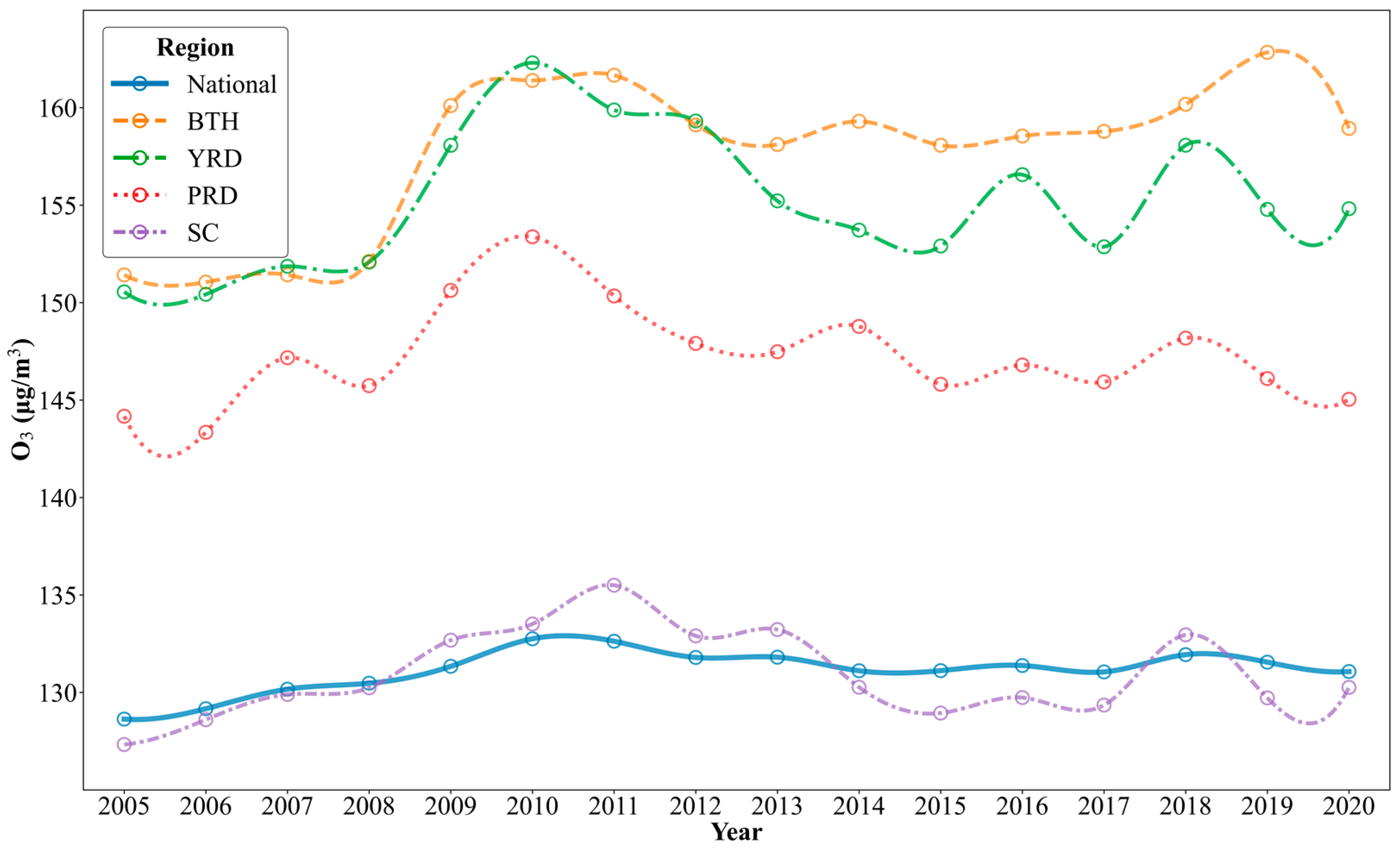
3.2. Time Variation of Ozone Concentrations

Figure 6 shows the time series of monthly average ozone concentrations of the whole country and four urban agglomerations from 2005 to 2020. Monthly variations in ozone concentrations are opposite to those of PM_2.5, showing an inverted “U” distribution. The highest concentration in China was 135.64 μg/m³ in June. The highest concentration in BTH was 201.85 μg/m³ in June. The highest concentration in the YRD was 174.9 μg/m³ in May. The highest concentration in the PRD was 167.37 μg/m³ in October. The highest concentration in SC was 140.07 μg/m³ in August. From the time-series chart, the change trends of the whole country, the YRDe, the PRD and SC are basically the same, while the Zui Yan of Pearl River Delta pollution is postponed to October. The national, YRD, BTH, and SC trends are basically the same, while the highest amount of pollution in the PRD is delayed until October.

As shown in Figure S1, the monthly time-series variations of the four indicators exhibit evident periodic fluctuations. These periodic changes are primarily attributed to seasonal variations in meteorological factors and anthropogenic pollutant emissions [49,50]. On the monthly scale, the monthly MC and PWC of O₃ range from 80.77 μg/m³ to 134.56 μg/m³ and 72.38 μg/m³ to 172.63 μg/m³, respectively (Figure S1a). Generally, the PWC is greater than MC, but the MC is higher than PWC in winter months (January and December), indicating that areas with relatively high O₃ concentrations in winter had lower population densities. PAE and PPE showed the same variation; however, in summer, PAE LT-2 and PPE LT-2 were as high as 90% and 99%, respectively (Figure S1b,c). The seasonal statistical results of the four indicators given in Table S1 also show that the seasonal characteristics of O₃ pollution are contrary to those of PM_2.5 in China; that is, the pollution is heavier in summer and relatively lighter in winter. High temperatures and strong radiation are the main meteorological factors causing O₃ pollution in summer [51].

Figure 7 shows the time-series variations in annual average ozone concentrations in China and the four urban agglomerations (the Yangtze River Delta (YRD), Pearl River Delta (PRD), Beijing–Tianjin–Hebei (BTH) and Sichuan–Chongqing urban agglomerations (SC)). In terms of time series, the pollution in BTH is the most serious, followed by the YRD; only the pollution level in SC is roughly the same as that in the whole country. Considering the possible differences in concentrations over time, we explored the differences in concentration trends from 2005 to 2012 and from 2013 to 2020 (Figure S2). The ozone concentrations in the five regions showed a significant growth trend from 2005 to 2012; the growth rate exceeded the national level. Between 2013 and 2020, the trend became chaotic and no regional trend passed the significance test. PWC and MC results show that PWC values were higher than MC values, indicating that high O₃ pollution occurred in areas with high population densities (Figure S3). The annual MC is highly consistent with the annual PWC in time series, showing a fluctuating upward trend; there are two peak points in the overall trend (2010 (MC: 130.97 μg/m³, PWC: 149.01 μg/m³) and 2018 (MC: 130.58 μg/m³, PWC: 146.95 μg/m³)). PAE is mostly concentrated between LT-1 and LT-2 (95.31% (2010) to 99.78% (2007)); the proportion of areas exceeding LT-2 is small (0.22% (2007) to 4.69% (2010)) (Figure S4a). It is noteworthy that PPE exceeded the LT-2 standard range from 5.59% (2006) to 40.37% (2010), indicating that the population density is high in areas where O₃ exceeded the standard (Figure S4b). Taking 2010 as an example, 40.37% of the national population lives in the areas exceeding the LT-2 standard by 4.69%. In general, the “seesaw” effect of changes in O₃ and PM_2.5 has not been effectively solved; thus, specific measures need to be taken to further strengthen ozone prevention and control.

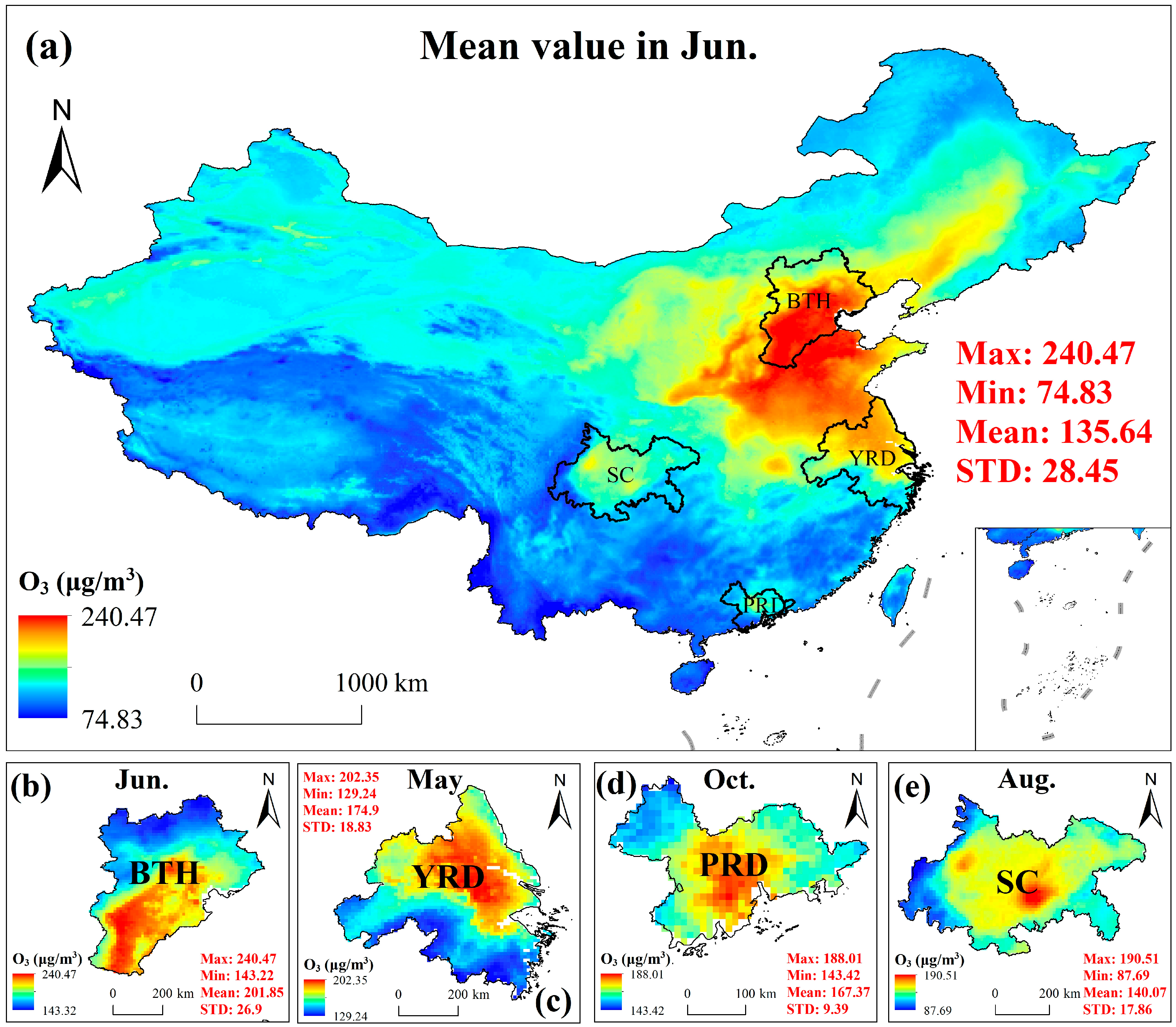
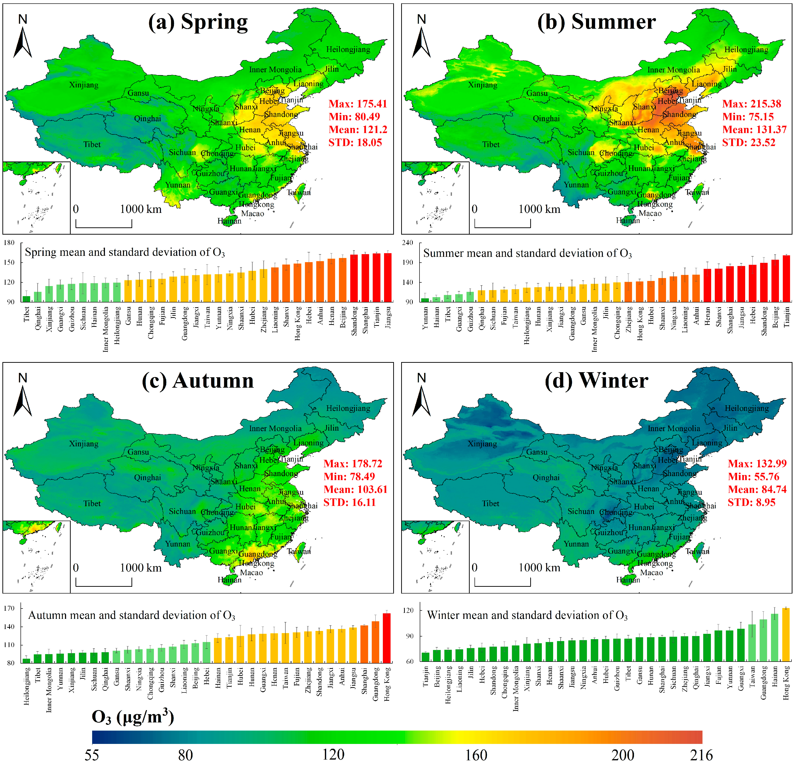
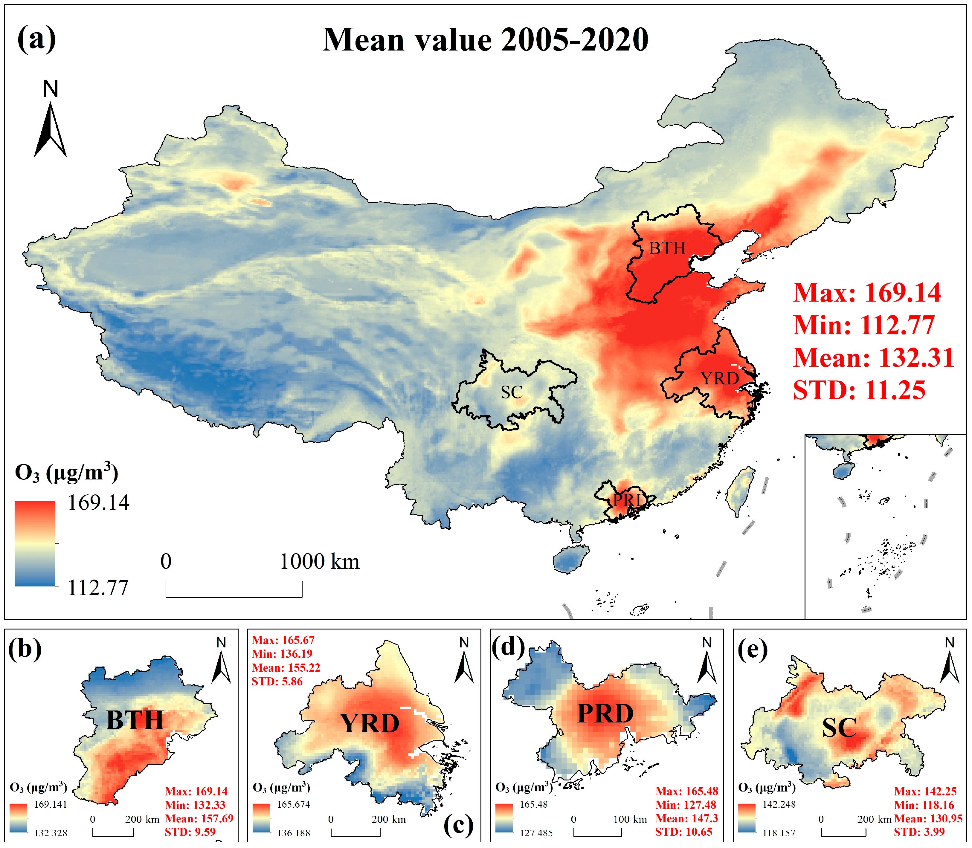
3.3. Spatial Distribution of Ozone Concentration

Figure 8 shows the spatial distribution of the months corresponding to the highest values of the time series in the five regions based on the results shown in Figure 6. The highest concentration in the national time series appeared in June, and the high pollution was distributed in the North China Plain (NCP), with the highest value of 240.47 μg/m³. The highest value in the YRD appeared in May and the highest value reached 202.35 μg/m³. The highest value in the PRD appeared in October and the highest value reached 188.01 μg/m³. The highest value in the BTH appeared in October and the highest value reached 188.01 μg/m³. The highest value in SC appeared in August and the highest value reached 190.51 μg/m³. The spatial distribution of the monthly concentrations can be seen more clearly in Figure S5. The ozone concentration changes in China show an inverted “U” shape, which is the opposite of PM_2.5. From the beginning of the year to the end of the year O₃ concentrations in China first showed an upward trend and then a downward trend. In January, O₃ concentrations were low (80.7 ± 10.56 μg/m³) and then began to increase, reaching the highest value in June (135.64 ± 28.45 μg/m³); O₃ concentration decreased to the lowest level in December (79.45 ± 12.11 μg/m³).

Figure 9 shows the seasonal spatial distribution of O₃ concentrations. O₃ concentrations in summer were the highest (131.37 ± 23.52 μg/m³); the extreme high value was concentrated in the NCP. Among the 33 provinces (Macao has no data), Tianjin, Beijing and Shandong were the most polluted areas (208.69 ± 2.16 μg/m³, 197.05 ± 13.18 μg/m³, 189.41 ± 13.7 μg/m³). O₃ concentrations in spring were the second highest (121.2 ± 18.05 μg/m³). Compared with summer, the most obvious change in O₃ concentrations in spring was in BTH (151.75 ± 14.5 μg/m³); however, BTH was still the most polluted region in the country. Jiangsu, Tianjin, and Shanghai were the most polluted provinces (164.41 ± 3.6 μg/m³, 163.87 ± 1.98 μg/m³, 162.93 ± 2.91 μg/m³). In autumn, the O₃ concentrations decreased gradually (103.61 ± 16.11 μg/m³); however, the O₃ concentrations in Guangdong Province showed an upward trend (summer: 129.34 ± 16.71 μg/m³; autumn: 149.21 ± 10.51 μg/m³) and ranked second in the histogram mean concentration, followed by Hong Kong. Compared with other seasons, O₃ concentrations in winter in China were satisfactory (84.74 ± 8.95 μg/m³); the BTH also showed satisfactory O₃ concentrations (76.04 ± 5.08 μg/m³). Of the 33 provinces, only 4 provinces exceeded the national primary standard (Hong Kong: 122.83 ± 1.44 μg/m³; Hainan: 116.43 ± 7.16 μg/m³; Guangdong: 109.78 ± 9.11 μg/m³; Taiwan: 103.99 ± 15.09 μg/m³).

Figure 10 shows the spatial distribution of the annual average ozone concentrations in China from 2005 to 2020, the partial enlarged map of YRD, PRD, BTH and SC. The average ozone concentration in China is 169.14 μg/m³. The most serious areas of ozone pollution are distributed in the NCP and the PRD. From the local enlarged map, the high value of pollution is concentrated in the built-up area with intensive human activities. From the spatial distribution of ozone concentrations in each year (Figure S6), the annual difference in the spatial distribution trend of ozone concentration is not obvious, indicating that there has been a lack of effective control measures for ozone. Using 2005 as the base year, the concentration difference between different years and the base year is displayed (Figure S7). It can be seen that in 2008 and before, the concentrations in most areas of China decreased slightly and that only some areas had an upward trend; however, since 2009, the concentration difference in the eastern region has risen rapidly, indicating that the pollution in the eastern region has deteriorated rapidly and that the deterioration trend has not been significantly alleviated.

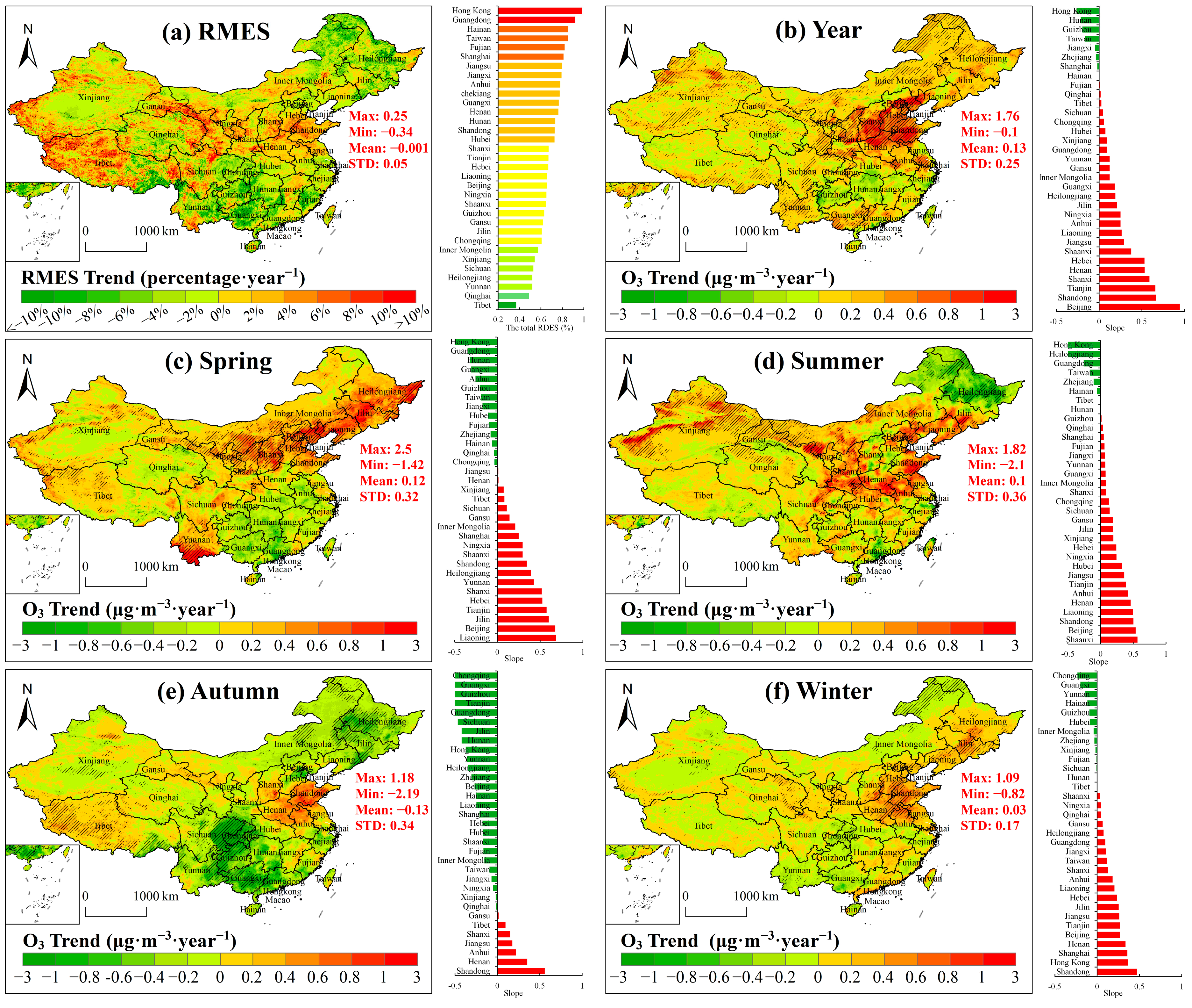
3.4. Spatial Variation of O₃ Concentration

The variation trend of O₃ concentrations and the proportions exceeding the standard in China are shown in Figure 11. Overall, the proportion of the over-standard area reached 68.84%. Hong Kong, Guangdong and Hainan were the most polluted areas because they had the highest rate of monthly O₃ concentrations exceeding the national standard (RMES) (98.15%, 91.51% and 85.4%). Tibet, Qinghai and Yunnan had the lightest pollution; the proportions exceeding the standard was only 36.91%, 48.87% and 51.86%, respectively. However, it should be noted that although Tibet is not highly polluted, the number of exceedances showed an upward trend. In addition, the proportions exceeding the standard in southwestern Xinjiang, Gansu Province, and the NCP also showed a rapid upward trend (Figure 11a). O₃ concentrations showed a significant upward trend in most regions of China, especially in the NCP and BTH. There is no significant downward trend in some parts of southern China and the Qinghai–Tibetan plateau. Among the 33 provinces, O₃ concentrations in 26 provinces showed an upward trend. Among them, Beijing, Shandong and Tianjin were the areas with the most serious air deterioration (0.946 μg/m³, 0.667 μg/m³, and 0.659 μg/m³ increase per year) (Figure 11b). The areas with the most serious pollution increases shifted to the Loess Plateau, northeast China and southwest Yunnan in spring. Liaoning, Beijing and Jilin were the three provinces with the most serious increase in pollution (0.686 μg·m⁻³·year⁻¹, 0.676 μg·m⁻³·year⁻¹, 0.601 μg·m⁻³·year⁻¹). Hong Kong, Guangdong, and Hunan in southern China had the largest decrease in O₃ concentrations (0.709 μg·m⁻³·year⁻¹, 0.349 μg·m⁻³·year⁻¹, and 0.322 μg·m⁻³·year⁻¹) (Figure 11c). The pollution in summer was serious; concentrations in 26 provinces showed an upward trend. The concentrations in Shanxi, Beijing and Shandong increased most rapidly (0.561 μg·m⁻³·year⁻¹, 0.536 μg·m⁻³·year⁻¹, and 0.502 μg·m⁻³⋅year⁻¹). Concentrations in Hong Kong, Heilongjiang and Guangdong decreased most rapidly (0.577 μg⋅m⁻³⋅year⁻¹, 0.567 μg⋅m⁻³⋅year⁻¹, and 0.258 μg⋅m⁻³⋅year⁻¹) (Figure 11d). The season with the most pronounced decline in O₃ was autumn; 26 provinces showed a downward trend. Specifically, Chongqing, Guangxi and Guizhou had the largest downward trend (1.1 μg⋅m⁻³⋅year⁻¹, 0.755 μg⋅m⁻³⋅year⁻¹, 0.707 μg⋅m⁻³⋅year⁻¹). Shandong, Henan and Anhui had the largest upward trend (0.558 μg⋅m⁻³⋅year⁻¹, 0.353 μg⋅m⁻³⋅year⁻¹, and 0.219 μg⋅m⁻³⋅year⁻¹) (Figure 11e). Although the variations in O₃ concentrations in winter are the smallest, it is still on the rise in the NCP. Among the 33 provinces, Shandong, Hong Kong and Shanghai have the largest upward trend (0.472 μg⋅m⁻³⋅year⁻¹, 0.365 μg⋅m⁻³⋅year⁻¹, and 0.356 μg⋅m⁻³⋅year⁻¹) (Figure 11f).

The change trends of the concentrations and the proportions of exceeding the standard in the four urban agglomerations were further analyzed (Figure S8). In the main urban area of each urban agglomeration, the proportion of concentrations exceeding the standard is mainly a downward trend, while in the periphery of the city, the proportion of concentrations exceeding the standard is mainly an upward trend. On the annual scale, the ozone concentrations in BTH have the strongest growth trend, with the highest value of 1.676 μg⋅m⁻³⋅year⁻¹. It is worth noting that, in addition to the PRD, the ozone concentrations in the built-up areas of the remaining three urban agglomerations mainly decrease in autumn. In other seasons, the opposite trend is seen among urban agglomerations.

4. Discussion

In order to solve the problem of the stability in the accuracy of the long-term modeling of O₃ concentrations, this study proposed a validated, residual, constrained random forest model (RF-RVC) for long-term O₃ concentration mapping. By constraining residuals to obtain limited samples for secondary modeling, the accuracy of O₃ mapping based on temporal validation is significantly improved at both annual and monthly scales. Compared with the RF-WRVC model, the RF-RVC model demonstrates stronger temporal transferability. The results show that the RF-RVC modeling accuracy is stable and reliable; there is no obvious overestimation or underestimation. Compared with previous studies, we did not perform secondary modeling on the residuals, but constrained the residuals, which is an innovative modeling approach and has been successfully applied to previous long-term satellite mapping of PM_2.5 concentrations [32]. In this study, the sample, station, and time-CV accuracies are 0.91, 0.90 and 0.86 at the monthly scale, and 0.87, 0.85 and 0.80 at the annual scale, respectively, which are comparable to those of previous long-term series mapping, but higher than those of previous short-term O₃ concentration models such as the GTWR model (CV R² = 0.79) [52], Bayesian maximum entropy–land-use mixed-effects regression (BME–LUR CV R² = 0.466) [53], and multiple linear regression-based eXtreme Gradient Boosting Machines (MLR-XGBM CV R² = 0.54) [48]. It should be emphasized that the RF model is not the focus of this study. The modeling idea of improving accuracy through residual constraints can be used for other models, regions and times. However, there are still limitations to the residual constraint modeling method. For example, the method assumes that the residual is normally distributed. However, the proportion of samples according to the two standard deviation thresholds in this study exceeds the threshold for normal distribution (4.55%). In addition, the elimination of extreme values also leads to some deviations in the estimation of extreme pollution events; that is, the underestimation of high values or overestimation of low values. Therefore, in future research, we will further optimize the residual threshold selection method and spatial–temporal scale effect, and apply the model to pollutants such as NO₂, SO₂, and CO.

O₃ concentrations in China show obvious seasonal variations, with high concentrations in summer and low concentrations in winter, which is opposite to PM_2.5 (Figure 9) [54]. The annual distribution of O₃ concentrations shown in Figure 7 and Figure S6 does not exhibit a significant downward trend. The trend of O₃ concentrations presented in Figure 11 indicates a concerning increase in concentrations. With regard to annual and seasonal concentrations, more than half of the provinces showed an upward trend in O₃ concentrations (except in autumn). High summer temperatures, strong solar radiation, and high surface temperatures are accompanied by high O₃ concentration; this has been widely recognized at global and regional scales [54,55,56]. This is because the precursors (e.g., NOx and VOCs) that have an important influence on O₃ will produce chemical reactions under high temperatures [12]; the generation of precursors are closely related to human activities. Therefore, in general, O₃ pollution is more serious in areas with intensive human activities, especially industrial activities (Figure 8 and Figure 10) [57]. It is worth mentioning that ozone concentrations in Guangdong Province are higher in autumn than in summer (Figure 6), which is inconsistent with the general performance in China, mainly due to the pollution transmission caused by monsoons [58,59]. As shown in Figure S4, the PAE and PPE showed an obvious upward trend from 2008 to 2010, which was consistent with the spatial and temporal variations in O₃ and its precursor pollutants in eastern China, based on OMI data analysis. It is also similar to the variation trend of NOx and O₃ based on ground observation and analysis in BTH [60,61]. As the main precursor pollutants of O₃, NOx is mainly produced by vehicle exhaust emissions and biomass burning. From relevant statistics and in the literature, we can see that from 2008 to 2010, the number of civilian vehicles in China was 50.9961 million, 62.8061 million, and 78.0183 million, respectively. The growth rates in 2009 and 2010 were 23.156% and 24.22%, respectively, while the number of newly registered civilian vehicles was 7.6318 million, 12.4595 million and 15.2882 million, respectively. The growth rate in 2009 was 63.26% higher than that in 2008. This dataset reveals some of the reasons for the significant increase in O₃ from 2008 to 2010.

The APPCAP has steadily reduced the PM_2.5 content in China but has failed to reduce the O₃ content (Figures S2 and S7). As shown in Figure S3, in the years following the initiation of the plan, both MC and PWC exhibited fluctuating trends; however, there was no obvious increase or decrease and the concentrations were always high. Although the content of nitrogen oxides has gradually decreased since 2013, emissions of non-methane volatile organic compounds (NMVOCs) have not been effectively controlled. Therefore, reducing O₃ pollution is still a challenging task [62,63]. The world is still experiencing global warming, which is accompanied by an increasing number of extreme weather events such as extreme high temperatures in summer [64,65]. These extreme meteorological events may exacerbate O₃ exposure, leading to more environmental health problems [54,66,67]. Figure S4 shows that the area proportion where PAE exceeds LT-2 is relatively small. Before 2009, PPE remained synchronized with PAE. However, starting in 2009, the area proportion of PPE exceeding LT-2 began to increase significantly and has remained around 40%, indicating that an increasing number of people are at risk of death from O₃ exposure [4]. Figure S1 shows that the MC in winter is higher than the PWC, which indicates that the decrease in MC cannot be synchronized with the PWC, which will further exacerbate the mortality risk associated with air pollution. Although existing studies have confirmed that pollution prevention and control measures have been successful in key areas, in non-key areas, serious health threats are still caused by excessive pollution exposure or population concentrations. Therefore, future research should pay more attention to human health-oriented air pollution intervention, especially in the non-priority areas of air pollution prevention and control [68].

Long-term mapping can understand the spatial and temporal variations in O₃ concentrations and identify potential pollution areas. For example, Figure S6 shows that the eastern coast, especially the NCP, has always been a severe region for O₃ pollution, with consistently high concentrations and no significant downward trend, which cannot be fully captured by station data. Thanks to the good performance of the residual correction idea, it is expected that data will be further extended to the daily or even hourly scale in future studies to observe the temporal variations in concentrations more carefully. In addition to obtaining O₃ concentration data over a large area, high spatial and temporal resolution pollutant modeling on a fine urban scale can be conducted using navigation data and micro-station data. Understanding the dynamic changes in O₃ in cities, identifying the hot spots of urban pollution, tracking the potential pollution sources, and forecasting future urban pollution in the short, medium and long term are of more practical significance for the prevention and control and control of urban pollution.

5. Conclusions

Considering that the traditional model cannot take into account the stability of long-time modeling, this study proposes a RF-RVC model based on residual standard deviation correction. The model eliminates abnormal samples through residual constraints, and obtains reliable model accuracy and stability through time-CV. The results of the long-time verification results show that the R² and RMSE of RF-RVC are better than those of RF-WRVC, which indicates that RF-RVC can better capture the nonlinear relationship between characteristic variables and O₃ and can effectively reduce the occurrence of various anomalies. At the same time, the monthly and annual time-CV accuracy of RF-RVC reached 0.86 and 0.80, and the model accuracy was improved by 24.64% and 35.59% compared with that of the RF-WRVC model. In a word, as an effective modeling idea, RF-RVC is expected to further improve modeling accuracy in other single models or stacked models, which will contribute to more accurate pollutant predictions.

References

1. Song, G.; Xing, J.; Yang, J.; Dong, L.; Lin, H.; Teng, M.; Hu, S.; Qin, Y.; Zeng, X. Surface UV-assisted retrieval of spatially continuous surface ozone with high spatial transferability. Remote Sens. Environ. 2022, 274, 112996. [Google Scholar] [CrossRef]
2. Fuhrer, J.; Booker, F. Ecological issues related to ozone: Agricultural issues. Environ. Int. 2003, 29, 141–154. [Google Scholar] [CrossRef] [PubMed]
3. Thurston, G.D.; Ito, K. Epidemiological studies of acute ozone exposures and mortality. J. Expo. Sci. Environ. Epidemiol. 2001, 11, 286–294. [Google Scholar] [CrossRef]
4. Malashock, D.A.; Delang, M.N.; Becker, J.S.; Serre, M.L.; West, J.J.; Chang, K.-L.; Cooper, O.R.; Anenberg, S.C. Global trends in ozone concentration and attributable mortality for urban, peri-urban, and rural areas between 2000 and 2019: A modelling study. Lancet Planet. Health 2022, 6, e958–e967. [Google Scholar] [CrossRef]
5. Liu, R.; Ma, Z.; Liu, Y.; Shao, Y.; Zhao, W.; Bi, J. Spatiotemporal distributions of surface ozone levels in China from 2005 to 2017: A machine learning approach. Environ. Int. 2020, 142, 105823. [Google Scholar] [CrossRef] [PubMed]
6. Li, M.; Yang, Q.; Yuan, Q.; Zhu, L. Estimation of high spatial resolution ground-level ozone concentrations based on Landsat 8 TIR bands with deep forest model. Chemosphere 2022, 301, 134817. [Google Scholar] [CrossRef]
7. Chen, C.; Zhang, P.; Yu, Y.; Hu, T. Development History and Future Prospects of Eco-environment Monitoring—From “Following” and “Running” to “Leading”. Environ. Prot. 2022, 50, 25–28. [Google Scholar]
8. Madaniyazi, L.; Nagashima, T.; Guo, Y.; Pan, X.; Tong, S. Projecting ozone-related mortality in East China. Environ. Int. 2016, 92–93, 165–172. [Google Scholar] [CrossRef]
9. Sun, Q.; Wang, W.; Chen, C.; Ban, J.; Xu, D.; Zhu, P.; He, M.Z.; Li, T. Acute effect of multiple ozone metrics on mortality by season in 34 Chinese counties in 2013–2015. J. Intern. Med. 2018, 283, 481–488. [Google Scholar] [CrossRef]
10. Zhu, S.; Tang, J.; Zhou, X.; Li, P.; Liu, Z.; Zhang, C.; Zou, Z.; Li, T.; Peng, C. Research progress, challenges, and prospects of PM2.5 concentration estimation using satellite data. Environ. Rev. 2023, 31, 605–631. [Google Scholar] [CrossRef]
11. Su, L.; Gao, C.; Ren, X.; Zhang, F.; Cao, S.; Zhang, S.; Chen, T.; Liu, M.; Ni, B.; Liu, M. Understanding the spatial representativeness of air quality monitoring network and its application to PM2.5 in the mainland China. Geosci. Front. 2022, 13, 101370. [Google Scholar] [CrossRef]
12. Wang, Y.; Yuan, Q.; Zhu, L.; Zhang, L. Spatiotemporal estimation of hourly 2-km ground-level ozone over China based on Himawari-8 using a self-adaptive geospatially local model. Geosci. Front. 2022, 13, 101286. [Google Scholar] [CrossRef]
13. Coyle, M.; Smith, R.; Stedman, J.; Weston, K.; Fowler, D. Quantifying the spatial distribution of surface ozone concentration in the UK. Atmos. Environ. 2002, 36, 1013–1024. [Google Scholar] [CrossRef]
14. Zhang, W.; Liu, D.; Tian, H.; Pan, N.; Yang, R.; Tang, W.; Yang, J.; Lu, F.; Dayananda, B.; Mei, H.; et al. Parsimonious estimation of hourly surface ozone concentration across China during 2015–2020. Sci. Data 2024, 11, 492. [Google Scholar] [CrossRef]
15. Skipper, T.N.; Hogrefe, C.; Henderson, B.H.; Mathur, R.; Foley, K.M.; Russell, A.G. Source-specific bias correction of US background and anthropogenic ozone modeled in CMAQ. Geosci. Model Dev. 2024, 17, 8373–8397. [Google Scholar] [CrossRef]
16. Sayahi, T.; Garff, A.; Quah, T.; Lê, K.; Becnel, T.; Powell, K.M.; Gaillardon, P.-E.; Butterfield, A.E.; Kelly, K.E. Long-term calibration models to estimate ozone concentrations with a metal oxide sensor. Environ. Pollut. 2020, 267, 115363. [Google Scholar] [CrossRef]
17. Chen, L.; Liang, S.; Li, X.; Mao, J.; Gao, S.; Zhang, H.; Sun, Y.; Vedal, S.; Bai, Z.; Ma, Z.; et al. A hybrid approach to estimating long-term and short-term exposure levels of ozone at the national scale in China using land use regression and Bayesian maximum entropy. Sci. Total Environ. 2021, 752, 141780. [Google Scholar] [CrossRef]
18. Babaan, J.; Hsu, F.-T.; Wong, P.-Y.; Chen, P.-C.; Guo, Y.-L.; Lung, S.-C.C.; Chen, Y.-C.; Wu, C.-D. A Geo-AI-based ensemble mixed spatial prediction model with fine spatial-temporal resolution for estimating daytime/nighttime/daily average ozone concentrations variations in Taiwan. J. Hazard. Mater. 2023, 446, 130749. [Google Scholar] [CrossRef] [PubMed]
19. Son, Y.; Osornio-Vargas, Á.R.; O’Neill, M.S.; Hystad, P.; Texcalac-Sangrador, J.L.; Ohman-Strickland, P.; Meng, Q.; Schwander, S. Land use regression models to assess air pollution exposure in Mexico City using finer spatial and temporal input parameters. Sci. Total Environ. 2018, 639, 40–48. [Google Scholar] [CrossRef]
20. Li, Z.; Wang, W.; He, Q.; Chen, X.; Huang, J.; Zhang, M. Estimating ground-level high-resolution ozone concentration across China using a stacked machine-learning method. Atmos. Pollut. Res. 2024, 15, 102114. [Google Scholar] [CrossRef]
21. Zhang, X.Y.; Zhao, L.M.; Cheng, M.M.; Chen, D.M. Estimating Ground-Level Ozone Concentrations in Eastern China Using Satellite-Based Precursors. IEEE Trans. Geosci. Remote Sens. 2020, 58, 4754–4763. [Google Scholar] [CrossRef]
22. Araki, S.; Hasunuma, H.; Yamamoto, K.; Shima, M.; Michikawa, T.; Nitta, H.; Nakayama, S.F.; Yamazaki, S. Estimating monthly concentrations of ambient key air pollutants in Japan during 2010–2015 for a national-scale birth cohort. Environ. Pollut. 2021, 284, 117483. [Google Scholar] [CrossRef] [PubMed]
23. Sihag, P.; Pandhiani, S.M.; Sangwan, V.; Kumar, M.; Angelaki, A. Estimation of ground-level O3 using soft computing techniques: Case study of Amritsar, Punjab State, India. Int. J. Environ. Sci. Technol. 2021, 19, 5563–5570. [Google Scholar] [CrossRef]
24. Gao, L.; Zhang, H.; Yang, F.; Tan, W.; Wu, R.; Song, Y. First estimation of hourly full-coverage ground-level ozone from Fengyun-4A Satellite using machine learning. Environ. Res. Lett. 2024, 19, 024040. [Google Scholar] [CrossRef]
25. Hsu, C.-Y.; Lee, R.-Q.; Wong, P.-Y.; Candice Lung, S.-C.; Chen, Y.-C.; Chen, P.-C.; Adamkiewicz, G.; Wu, C.-D. Estimating morning and evening commute period O3 concentration in Taiwan using a fine spatial-temporal resolution ensemble mixed spatial model with Geo-AI technology. J. Environ. Manag. 2024, 351, 119725. [Google Scholar] [CrossRef]
26. Wei, J.; Li, Z.; Li, K.; Dickerson, R.R.; Pinker, R.T.; Wang, J.; Liu, X.; Sun, L.; Xue, W.; Cribb, M. Full-coverage mapping and spatiotemporal variations of ground-level ozone (O3) pollution from 2013 to 2020 across China. Remote Sens. Environ. 2022, 270, 112775. [Google Scholar] [CrossRef]
27. Chen, B.; Zheng, Q.; Sun, W.; Yang, G.; Feng, T.; Wang, Y. Geo-STO3Net: A deep neural network integrating geographical spatiotemporal information for surface ozone estimation. IEEE Trans. Geosci. Remote Sens. 2024, 62, 1–14. [Google Scholar] [CrossRef]
28. He, Q.; Huang, B. Satellite-based mapping of daily high-resolution ground PM2.5 in China via space-time regression modeling. Remote Sens. Environ. 2018, 206, 72–83. [Google Scholar] [CrossRef]
29. Ma, Z.; Hu, X.; Sayer, A.M.; Levy, R.; Zhang, Q.; Xue, Y.; Tong, S.; Bi, J.; Huang, L.; Liu, Y. Satellite-Based Spatiotemporal Trends in PM2.5 Concentrations: China, 2004–2013. Environ. Health Perspect. 2016, 124, 184–192. [Google Scholar] [CrossRef]
30. Fang, X.; Zou, B.; Liu, X.; Sternberg, T.; Zhai, L. Satellite-based ground PM2.5 estimation using timely structure adaptive modeling. Remote Sens. Environ. 2016, 186, 152–163. [Google Scholar] [CrossRef]
31. Lee, H.J.; Liu, Y.; Coull, B.A.; Schwartz, J.; Koutrakis, P. A novel calibration approach of MODIS AOD data to predict PM2.5 concentrations. Atmos. Chem. Phys. 2011, 11, 7991–8002. [Google Scholar] [CrossRef]
32. Li, S.; Zou, B.; Fang, X.; Lin, Y. Time series modeling of PM2.5 concentrations with residual variance constraint in eastern mainland China during 2013–2017. Sci. Total Environ. 2020, 710, 135755. [Google Scholar] [CrossRef] [PubMed]
33. Ma, Z.; Hu, X.; Huang, L.; Bi, J.; Liu, Y. Estimating Ground-Level PM2.5 in China Using Satellite Remote Sensing. Environ. Sci. Technol. 2014, 48, 7436–7444. [Google Scholar] [CrossRef] [PubMed]
34. Ministry of Ecology and Environment (MEE). Revision of the Ambient Air Quality Standards (GB 3095-2012). 2018. Available online: https://www.mee.gov.cn/gkml/sthjbgw/sthjbgg/201808/t20180815_451398.htm (accessed on 11 April 2025). (In Chinese)
35. Lamsal, L.N.; Krotkov, N.A.; Vasilkov, A.; Marchenko, S.; Qin, W.; Yang, E.-S.; Fasnacht, Z.; Joiner, J.; Choi, S.; Haffner, D.; et al. Ozone Monitoring Instrument (OMI) Aura nitrogen dioxide standard product version 4.0 with improved surface and cloud treatments. Atmos. Meas. Tech. 2021, 14, 455–479. [Google Scholar] [CrossRef]
36. Levelt, P.F.; Van Den Oord, G.H.; Dobber, M.R.; Malkki, A.; Visser, H.; De Vries, J.; Stammes, P.; Lundell, J.O.; Saari, H. The ozone monitoring instrument. IEEE Trans. Geosci. Remote Sens. 2006, 44, 1093–1101. [Google Scholar] [CrossRef]
37. Li, K.; Jacob, D.J.; Shen, L.; Lu, X.; De Smedt, I.; Liao, H. Increases in surface ozone pollution in China from 2013 to 2019: Anthropogenic and meteorological influences. Atmos. Chem. Phys. 2020, 20, 11423–11433. [Google Scholar] [CrossRef]
38. He, J.; Gong, S.; Yu, Y.; Yu, L.; Wu, L.; Mao, H.; Song, C.; Zhao, S.; Liu, H.; Li, X.; et al. Air pollution characteristics and their relation to meteorological conditions during 2014–2015 in major Chinese cities. Environ. Pollut. 2017, 223, 484–496. [Google Scholar] [CrossRef]
39. Meleux, F.; Solmon, F.; Giorgi, F. Increase in summer European ozone amounts due to climate change. Atmos. Environ. 2007, 41, 7577–7587. [Google Scholar] [CrossRef]
40. Dickerson, R.R.; Li, C.; Li, Z.; Marufu, L.T.; Stehr, J.W.; McClure, B.; Krotkov, N.; Chen, H.; Wang, P.; Xia, X.; et al. Aircraft observations of dust and pollutants over northeast China: Insight into the meteorological mechanisms of transport. J. Geophys. Res. Atmos. 2007, 112, D24S90. [Google Scholar] [CrossRef]
41. Reed, F.J.; Gaughan, A.E.; Stevens, F.R.; Yetman, G.; Sorichetta, A.; Tatem, A.J. Gridded Population Maps Informed by Different Built Settlement Products. Data 2018, 3, 33. [Google Scholar] [CrossRef]
42. Witte, J.C.; Duncan, B.N.; Douglass, A.R.; Kurosu, T.P.; Chance, K.; Retscher, C. The unique OMI HCHO/NO2 feature during the 2008 Beijing Olympics: Implications for ozone production sensitivity. Atmos. Environ. 2011, 45, 3103–3111. [Google Scholar] [CrossRef]
43. Shith, S.; Ramli, N.A.; Awang, N.R.; Ismail, M.R.; Latif, M.T.; Zainordin, N.S. Does Light Pollution Affect Nighttime Ground-Level Ozone Concentrations? Atmosphere 2022, 13, 1844. [Google Scholar] [CrossRef]
44. Chen, Z.; Yu, B.; Yang, C.; Zhou, Y.; Yao, S.; Qian, X.; Wang, C.; Wu, B.; Wu, J. An extended time series (2000–2018) of global NPP-VIIRS-like nighttime light data from a cross-sensor calibration. Earth Syst. Sci. Data 2021, 13, 889–906. [Google Scholar] [CrossRef]
45. Liu, N.; Zou, B.; Zhang, H. Uncertainty measuring and constraining method for geographic weighted regression model results. Acta Geod. Cartogr. Sin. 2023, 52, 307–317. [Google Scholar]
46. Breiman, L. Some Infinity Theory for Predictor Ensembles. University of California at Berkeley Papers. 2000. Available online: https://www.google.com/url?sa=t&source=web&rct=j&opi=89978449&url=https://www.stat.berkeley.edu/~breiman/some_theory2000.pdf&ved=2ahUKEwiP9dD9pfOMAxWas1YBHXUQKjgQFnoECCAQAQ&usg=AOvVaw0cirbK88sm1LYVgxZ2e0zp (accessed on 11 April 2025).
47. Kang, Y.; Choi, H.; Im, J.; Park, S.; Shin, M.; Song, C.-K.; Kim, S. Estimation of surface-level NO2 and O3 concentrations using TROPOMI data and machine learning over East Asia. Environ. Pollut. 2021, 288, 117711. [Google Scholar] [CrossRef] [PubMed]
48. Li, R.; Cui, L.; Hongbo, F.; Li, J.; Zhao, Y.; Chen, J. Satellite-based estimation of full-coverage ozone (O3) concentration and health effect assessment across Hainan Island. J. Clean. Prod. 2020, 244, 118773. [Google Scholar] [CrossRef]
49. Zheng, Q.; Shi, J.; Tan, J.; Duan, Y.; Lin, Y.; Xu, W. Characteristics of Aerosol Particulate Concentrations and Their Climate Background in Shanghai During 2007–2016. Environ. Sci. 2020, 41, 14–22. [Google Scholar]
50. Qian, Y.; Xu, B.; Xia, L.; Chen, Y.; Deng, L.; Wang, H.; Zhang, G. Characteristics of Ozone Pollution and Relationships with Meteorological Factors in Jiangxi Province. Environ. Sci. 2021, 42, 2190–2201. [Google Scholar]
51. Wang, L.; Chen, B.; Ouyang, J.; Mu, Y.; Zhen, L.; Yang, L.; Xu, W.; Tang, L. Causal-inference machine learning reveals the drivers of China’s 2022 ozone rebound. Environ. Sci. Ecotechnol. 2025, 24, 100524. [Google Scholar] [CrossRef]
52. Pan, J.; Li, X.; Zhu, S. High-resolution estimation of near-surface ozone concentration and population exposure risk in China. Environ. Monit. Assess. 2024, 196, 249. [Google Scholar] [CrossRef]
53. Adam-Poupart, A.; Brand, A.; Fournier, M.; Jerrett, M.; Smargiassi, A. Spatiotemporal Modeling of Ozone Levels in Quebec (Canada): A Comparison of Kriging, Land-Use Regression (LUR), and Combined Bayesian Maximum Entropy–LUR Approaches. Environ. Health Perspect. 2014, 122, 970–976. [Google Scholar] [CrossRef] [PubMed]
54. Liu, X.; Zhu, Y.; Xue, L.; Desai, A.R.; Wang, H. Cluster-Enhanced Ensemble Learning for Mapping Global Monthly Surface Ozone From 2003 to 2019. Geophys. Res. Lett. 2022, 49, e2022GL097947. [Google Scholar] [CrossRef]
55. Lee, Y.C.; Shindell, D.T.; Faluvegi, G.; Wenig, M.; Lam, Y.F.; Ning, Z.; Hao, S.; Lai, C.S. Increase of ozone concentrations, its temperature sensitivity and the precursor factor in South China. Tellus B Chem. Phys. Meteorol. 2014, 66, 23455. [Google Scholar] [CrossRef]
56. Antón, M.; Loyola, D.; Clerbaux, C.; López, M.; Vilaplana, J.M.; Bañón, M.; Hadji-Lazaro, J.; Valks, P.; Hao, N.; Zimmer, W.; et al. Validation of the MetOp-A total ozone data from GOME-2 and IASI using reference ground-based measurements at the Iberian Peninsula. Remote Sens. Environ. 2011, 115, 1380–1386. [Google Scholar] [CrossRef]
57. Ding, S.; He, J.; Liu, D. Investigating the biophysical and socioeconomic determinants of China tropospheric O3 pollution based on a multilevel analysis approach. Environ. Geochem. Health 2021, 43, 2835–2849. [Google Scholar] [CrossRef]
58. Cao, T.; Wang, H.; Li, L.; Lu, X.; Liu, Y.; Fan, S. Fast spreading of surface ozone in both temporal and spatial scale in Pearl River Delta. J. Environ. Sci. 2024, 137, 540–552. [Google Scholar] [CrossRef]
59. Chen, Y.; Tong, L.; Yu, W.; Jin, S.; Yuhong, Z.; Siqi, Y.; Duohong, C.; Jingyang, C. Characteristics of Ozone Pollution in Guangdong Province from 2016 to 2020. Ecol. Environ. Sci. 2022, 31, 2374–2381. [Google Scholar]
60. Yang, J.; Xin, J.; Dongsheng, J.; Bin, Z. Variation Analysis of Background Atmospheric Pollutants in North China During the Summer of 2008 to 2011. Environ. Sci. 2012, 33, 3693–3704. [Google Scholar]
61. Shan, Y.; Li, L.; Qiong, L.; Yonghang, C.; Yingying, S.; Xiaozheng, L.; Liping, Q. Spatial-Temporal Distribution of Ozone and Its Precursors over Central and Eastern China based on OMI Data. Res. Environ. Sci. 2016, 29, 1128–1136. [Google Scholar]
62. Ding, S.; Wei, Z.; Liu, S.; Zhao, R. Uncovering the evolution of ozone pollution in China: A spatiotemporal characteristics reconstruction from 1980 to 2021. Atmos. Res. 2024, 307, 107472. [Google Scholar] [CrossRef]
63. Zheng, B.; Tong, D.; Li, M.; Liu, F.; Hong, C.; Geng, G.; Li, H.; Li, X.; Peng, L.; Qi, J.; et al. Trends in China’s anthropogenic emissions since 2010 as the consequence of clean air actions. Atmos. Chem. Phys. 2018, 18, 14095–14111. [Google Scholar] [CrossRef]
64. Lu, R.; Xu, K.; Chen, R.; Chen, W.; Li, F.; Lv, C. Heat waves in summer 2022 and increasing concern regarding heat waves in general. Atmos. Ocean. Sci. Lett. 2023, 16, 100290. [Google Scholar] [CrossRef]
65. Ji, P.; Yuan, X.; Ma, F.; Xu, Q. Drivers of long-term changes in summer compound hot extremes in China: Climate change, urbanization, and vegetation greening. Atmos. Res. 2024, 310, 107632. [Google Scholar] [CrossRef]
66. Pascal, M.; Wagner, V.; Alari, A.; Corso, M.; Le Tertre, A. Extreme heat and acute air pollution episodes: A need for joint public health warnings? Atmos. Environ. 2021, 249, 118249. [Google Scholar] [CrossRef]
67. Liu, X.; Desai, A.R. Significant Reductions in Crop Yields From Air Pollution and Heat Stress in the United States. Earth Future 2021, 9, e2021EF002000. [Google Scholar] [CrossRef]
68. Zou, B.; You, J.; Lin, Y.; Duan, X.; Zhao, X.; Fang, X.; Campen, M.J.; Li, S. Air pollution intervention and life-saving effect in China. Environ. Int. 2019, 125, 529–541. [Google Scholar] [CrossRef]
Figure 1. Distribution of ground-based air-quality monitoring stations.
Remotesensing 17 01534 g001
Figure 2. Schematic representation of the results of statistical modelling: (a) in general; (b) Cases with outliers; blue point: general sample; orange point: abnormal point.
Remotesensing 17 01534 g002
Figure 3. Schematic diagram of error distribution curve.
Remotesensing 17 01534 g003
Figure 4. RF-RVC technology flowchart.
Remotesensing 17 01534 g004
Figure 5. The optimal RF-RVC model is based on time validation results: (a) monthly scale; (b) yearly scale.
Remotesensing 17 01534 g005
Figure 6. Line chart of monthly average ozone concentrations.
Remotesensing 17 01534 g006
Figure 7. Line chart of annual average ozone concentrations.
Remotesensing 17 01534 g007
Figure 8. Spatial distribution of the months with the highest monthly mean ozone concentrations in each region from 2005 to 2020: (a) nationwide; (b) YRD; (c) PRD; (d) BTH; and (e) SC.
Remotesensing 17 01534 g008
Figure 9. Spatial distribution of multi-year seasonal mean of O3 concentration in China from 2005 to 2020: (a) spring; (b) summer; (c) autumn; and (d) winter.
Remotesensing 17 01534 g009
Figure 10. Distribution and broken line statistical chart of annual mean ozone from 2005 to 2020: (a) nationwide; (b) YRD; (c) PRD; (d) BTH; and (e) SC.
Remotesensing 17 01534 g010
Figure 11. Spatial distribution of annual exceeding standard proportion and variation trend of annual O3 concentrations: (a) RMES; (b) year; (c) spring; (d) summer; (e) autumn; and (f) winter. Note: the slash in the figure indicates the trend significant area (p < 0.05).
Remotesensing 17 01534 g011