Comparative Analysis of Novel View Synthesis and Photogrammetry for 3D Forest Stand Reconstruction and Extraction of Individual Tree Parameters

Abstract

The accurate and efficient 3D reconstruction of trees is beneficial for urban forest resource assessment and management. Close-range photogrammetry (CRP) is widely used in the 3D model reconstruction of forest scenes. However, in practical forestry applications, challenges such as low reconstruction efficiency and poor reconstruction quality persist. Recently, novel view synthesis (NVS) technology, such as neural radiance fields (NeRF) and 3D Gaussian splatting (3DGS), has shown great potential in the 3D reconstruction of plants using some limited number of images. However, existing research typically focuses on small plants in orchards or individual trees. It remains uncertain whether this technology can be effectively applied in larger, more complex stands or forest scenes. In this study, we collected sequential images of urban forest plots with varying levels of complexity using imaging devices with different resolutions (cameras on smartphones and UAV). These plots included one with sparse, leafless trees and another with dense foliage and more occlusions. We then performed dense reconstruction of forest stands using NeRF and 3DGS methods. The resulting point cloud models were compared with those obtained through photogrammetric reconstruction and laser scanning methods. The results show that compared to photogrammetric method, NVS methods have a significant advantage in reconstruction efficiency. The photogrammetric method is suitable for relatively simple forest stands, as it is less adaptable to complex ones. This results in tree point cloud models with issues such as excessive canopy noise and wrongfully reconstructed trees with duplicated trunks and canopies. In contrast, NeRF is better adapted to more complex forest stands, yielding tree point clouds of the highest quality that offer more detailed trunk and canopy information. However, it can lead to reconstruction errors in the ground area when the input views are limited. The 3DGS method has a relatively poor capability to generate dense point clouds, resulting in models with low point density, particularly with sparse points in the trunk areas, which affects the accuracy of the diameter at breast height (DBH) estimation. Tree height and crown diameter information can be extracted from the point clouds reconstructed by all three methods, with NeRF achieving the highest accuracy in tree height. However, the accuracy of DBH extracted from photogrammetric point clouds is still higher than that from NeRF point clouds. Meanwhile, compared to ground-level smartphone images, tree parameters extracted from reconstruction results of higher-resolution and varied perspectives of drone images are more accurate. These findings confirm that NVS methods have significant application potential for 3D reconstruction of urban forests.

1. Introduction

Forests occupy a significant portion of urban landscapes, serving as a critical component of urban ecosystems [1]. They can mitigate urban heat island effects, improve air quality, and provide essential environmental and ecosystem services [2]. Tree parameters such as tree height (TH), diameter at breast height (DBH), crown diameter (CD), crown width, and above-ground biomass effectively reflect the growth conditions, spatial distribution, and structural features of urban forest resources [3]. They also serve as important indicators for measuring the carbon sequestration capacity of urban forests and assessing urban ecological functions [4].

The traditional method for obtaining tree parameters in forest stands involves manual measurements, such as using calipers or diameter tapes to measure the DBH and hypsometers to measure TH, followed by recording and organizing the results. Many researchers consider this method as time-consuming and labor-intensive [5,6,7], particularly for large-scale surveys (e.g., urban forest parks). Additionally, the measurement results are prone to being influenced by human subjective factors [6]. For instance, in a study of 319 trees in the Evo area of southern Finland, four trained surveyors independently measured the DBH and TH using calipers and clinometers. However, differences in the way the surveyors used the calipers resulted in variations in the measurement results [8]. 3D reconstruction technology can convert forest scenes into 3D digital models and obtain tree properties from these models using automated procedures instead of manual measurements to improve work efficiency and reduce bias [9]. In addition, tree models constructed from 3D point clouds can be used for the planning and management of green infrastructure in the development of smart cities [10].

The terrestrial laser scanner (TLS) has been used to obtain high-density 3D point cloud models of forest scenes, from which parameters such as TH and DBH can be derived for individual trees [11,12,13]. Meanwhile, tree structural parameters derived from TLS have been proven to be highly reliable. Reddy, et al. [14] validated the DBH and TH estimates automatically derived by TLS in deciduous forests. Compared to field measurements, the DBH had an R² = 0.96 and RMSE = 4.1 cm, while the height estimate had an R² = 0.98 and RMSE = 1.65 m. Due to the high measurement accuracy of TLS, it can also be used as a benchmark for other remote sensing methods instead of field survey data [15,16]. However, because of the limited scanning angles of TLS and occlusion effects, it is challenging to capture complete canopy information for taller parts of trees. Therefore, airborne laser scanners are commonly used to collect canopy point cloud data. Jaskierniak, et al. [17] utilized an airborne laser scanning (ALS) system to acquire point cloud data of structurally complex mixed forests and performed individual tree detection and canopy delineation. Liao, et al. [18] investigated the role of ALS data in improving the accuracy of tree volume estimation. Their study demonstrated that THs extracted from ALS data are more accurate than those measured manually with a telescoping pole. Combining ALS data with on-site DBH measurements effectively improves the accuracy of tree volume estimates. Although TLS and ALS can acquire large-area point cloud data in a short period, these devices are expensive and require high levels of technical expertise to operate [19]. Additionally, in many countries flight permits are required for uncrewed aerial vehicle (UAV) operators to carry out drone flights.

With the advancement of image processing algorithms, camera sensors and hardware, close-range photogrammetry (CRP) is now considered as a cost-effective alternative to laser scanning in 3D reconstruction. The CRP method has demonstrated significant potential in urban forest survey works [20,21,22], as 3D point cloud can be reconstructed from overlapping images. This allows for the acquisition of 3D model information of trees using only forest scene imagery which is easily available. Compared to TLS and ALS, CRP significantly reduces costs and operational complexity. The current mainstream photogrammetry method is structure from motion (SfM) [23] + multi-view stereo (MVS) [24], which involves feature detection, feature matching, and depth fusion between image pairs. SfM uses matching constraints and triangulation principles to obtain 3D sparse point and camera parameters, while MVS densifies the point cloud. Kameyama and Sugiura [25] used UAV to capture forest images under different conditions, employed the SfM method to create 3D models, and validated the measurement accuracy of tree height and volume. Bayati, et al. [26] used hand-held digital cameras and SfM-MVS to produce a 3D reconstruction of uneven-aged deciduous forests and successfully extracted individual tree DBH. A high coefficient of the determinant (R²  =  98%) was observed between DBH derived from field measurements and that from the SfM-MVS technique. Xu, et al. [27] compared the accuracy of forest structure parameters extracted from SfM and Backpack LiDAR Scanning (BLS) point clouds. Their results showed that SfM point cloud models are well-suited for extracting DBH, but there is still a gap in the accuracy of TH extraction. This discrepancy depends on the quality of the point cloud model, which is influenced not only by the robustness of the algorithm but also by the quality of the acquired images and feature matching. In complex forest environments, there are often occlusions and varying lighting conditions between trees, which affect the quality of image data. Furthermore, similar shape and texture patterns between trees pose challenges for feature matching. To improve the quality of forest scene images, Zhu, et al. [28] compared three image enhancement algorithms and concluded that the multi-scale retinex algorithm is more suitable for 3D reconstruction of forest scenes. Although these enhancements can improve the quality of forest scene reconstruction to some extent, there are still discrepancies in data accuracy compared to that obtained from TLS, and there remains significant room for improvement in terms of time efficiency.

Recently, novel view synthesis (NVS) technology has become an active research topic in computer vision. Mildenhall, et al. [29] first introduced a deep learning-based rendering method called neural radiance fields (NeRF). NeRF implicitly renders complex static scenes in 3D using a fully connected network. Since then, NeRF has drawn the attention of many researchers, leading to various improvements. Müller, et al. [30] introduced a hash mapping technique to enhance the sampling point positional encoding method, effectively accelerating network training. In terms of reconstruction accuracy, Barron, et al. [31] used conical frustums instead of ray sampling to address aliasing issues at different distances. Wang, et al. [32] replaced the multi-layer perceptron (MLP) with signed distance functions (SDF) for geometric representation, achieving high-precision geometric reconstruction. These improvements have pushed research on NeRF into practical applications, providing high-quality 3D rendering perspectives for fields like autonomous driving [33] and 3D city modeling [34]. NeRF is not only capable of synthesizing novel view images but can also be used to reconstruct 3D models. Currently reported applications in 3D reconstruction include cultural heritage [35] and plants and trees. In the context of plant 3D reconstruction and phenotypic research, Hu, et al. [36] evaluated the application of NeRF in the 3D reconstruction of low-growing plants. The results demonstrated that NeRF introduces a new paradigm in plant phenotypic analysis, providing a powerful tool for 3D reconstruction. Zhang, et al. [37] proposed the NeRF-Ag model, which realized the 3D reconstruction of orchard scenes and effectively improved the modeling accuracy and efficiency. Huang, et al. [38] evaluated NeRF’s ability to generate dense point clouds for individual trees of varying complexity, providing a novel example for NeRF-based single tree reconstruction. Nevertheless, NeRF still faces challenges in achieving high-resolution real-time rendering and efficient dynamic scene editing. 3D Gaussian splatting (3DGS) [39] brought a technological breakthrough to the field. Unlike NeRF, 3DGS utilizes an explicit Gaussian point representation to precisely capture and present information about 3D scenes. In terms of optimization and rendering speed, 3DGS significantly outperforms the original NeRF method [40], advancing NVS technology to a new level. The results of the 3DGS algorithm were compared with the state-of-the-art Mip-NeRF360 method and performed better on standard metrics [41]. 3DGS technology has become a transformative force driving innovations in related fields, with notable achievements in areas such as novel view rendering [42] and dynamic scene reconstruction [43]. However, the application of 3DGS to plants and forest scenes reconstruction and the generation of dense point cloud models of trees have not yet been fully explored and evaluated.

Compared to individual trees, forest stands consisting of multiple trees exhibit substantial self-occlusion and increasing complexity, posing greater challenges for image acquisition and 3D reconstruction. Research on the application of NVS technology in this area remains scarce, lacking a complete reconstruction workflow and detailed evaluation results. Therefore, this study applies NeRF and 3DGS technologies to the 3D reconstruction of trees in urban forest stands to obtain dense 3D point cloud models. The generated point cloud models are then compared and evaluated against photogrammetric methods using TLS point cloud as reference. The specific research objectives are as follows:

(1)

Comparing the practical application of NVS techniques and photogrammetric reconstruction methods in complex urban forest stands;

(2)

Evaluating the ability of different NVS methods (one based on implicit neural networks: NeRF; another on explicit Gaussian point clouds: 3DGS) in reconstructing trees and generating dense point clouds;

(3)

Comparing tree parameters extracted from various 3D point cloud models and assessing whether NVS techniques can replace or supplement photogrammetric methods, potentially becoming a new tool for forest scene reconstruction and forest resource surveys.

2. Materials and Method

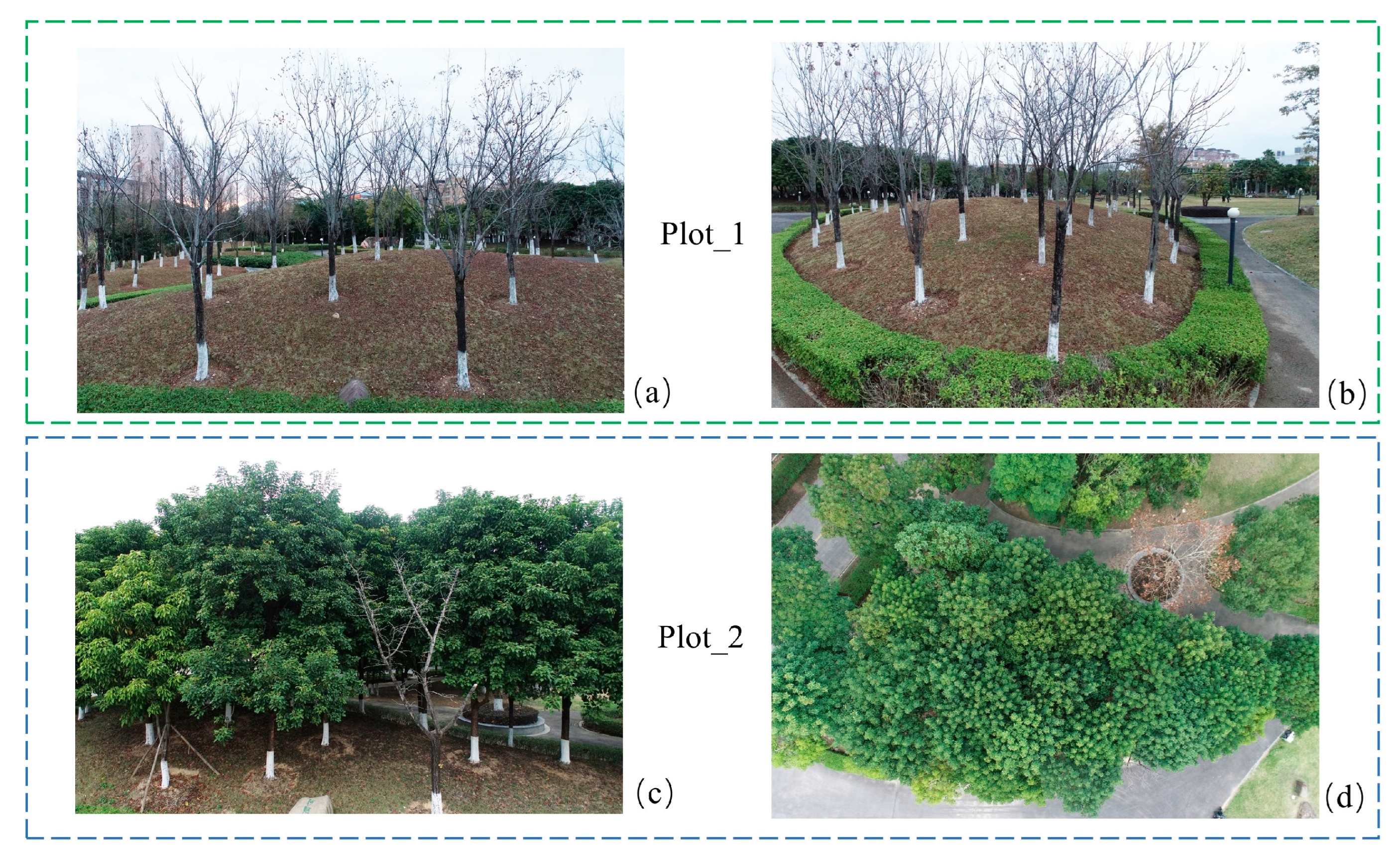
2.1. Study Area

We selected two contrasting urban forest plots in the Qishan campus of Fuzhou University to conduct this experiment. Plot_1 is an irregularly elongated circular area with a topography that is higher in the center and lower at the edges, exhibiting an elevation difference of 2.4 m. It is located in an open area with minimal surrounding vegetation, which facilitates effective image data collection. There are 45 golden rain trees (Koelreuteria bipinnata ‘integrifoliola’) within the plot. During data collection, which occurred in the winter leaf-off period, the tree trunks and the canopies are clearly visible. The TH ranges from 4 to 11 m (average: 7.5 m), and the DBH ranges from 15 to 23 cm (average: 16.7 cm). Plot_2 is also an irregularly shaped area with a similar topography, being higher in the center and lower at the edges, exhibiting an elevation difference of 2.2 m. One side of the plot is relatively open, while the other side is densely occupied with other trees, presenting challenges for image acquisition. The predominant tree species is the autumn maple tree (Bischofia javanica Blume), an evergreen broadleaf tree. Compared to the trees in Plot_1, the plot features 33 trees with greater height variation, larger canopy size, and dense foliage. The TH ranges from 7 to 12 m (average: 9.4 m), and the DBH ranges from 16 to 27 cm (average: 21.2 cm). Figure 1 shows the morphology of the study plots. For the research objectives, we selected forest stand plots with different tree types and canopy structures (leafless vs. leafy) to study how these factors might affect the reconstruction results.

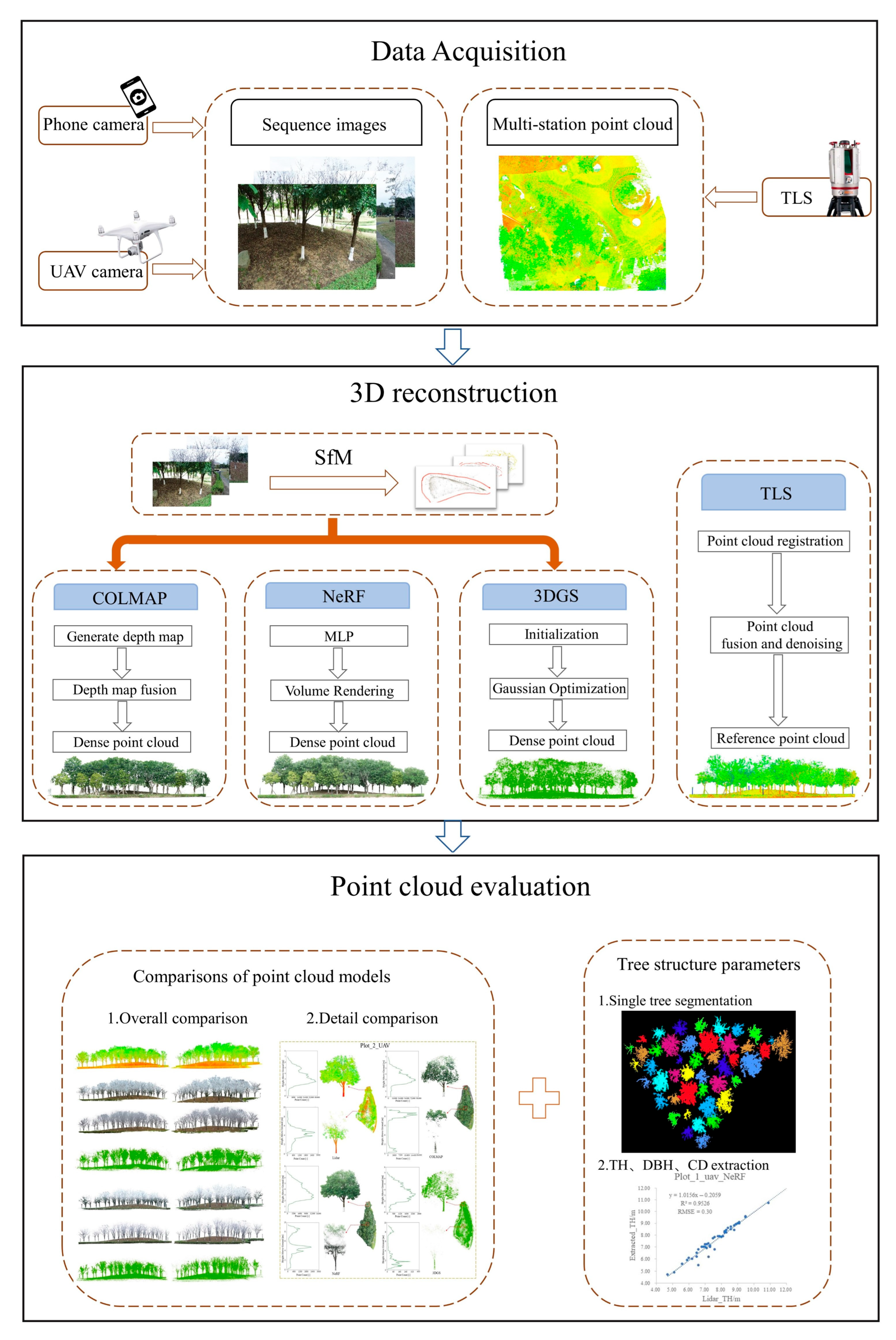
2.2. Research Method

2.2.1. Photogrammetric Reconstruction

Photogrammetric reconstruction based on computer vision has become a mature processing routine. Structure from motion (SfM) and multi-view stereo (MVS) are the two main steps. COLMAP (Version 3.8, https://colmap.github.io/ (accessed on 3 June 2024)) is a widely used open-source SfM + MVS program in 3D reconstruction research, and we used it to conduct photogrammetric reconstruction experiments. In COLMAP’s SfM process, the scale-invariant feature transform (SIFT) feature extraction algorithm is used to identify feature points from images, which are then matched using spatial matching algorithms, with points not meeting geometric constraints filtered out. Finally, bundle adjustment is performed to obtain camera pose parameters and a sparse point cloud. The MVS module in COLMAP employs an improved patch match MVS algorithm to estimate depth maps based on the sparse reconstruction results and fuses them to generate a dense point cloud. Both NeRF and 3DGS also rely on calibrated images, camera pose parameters, and sparse point clouds generated by COLMAP’s SfM module as initial inputs for training.

2.2.2. Neural Radiance Fields (NeRF)

The original NeRF represents an entire scene using a multi-layer perceptron (MLP) as an implicit function, consisting of an 8-layer spatial network and a 4-layer view network, with each layer typically having 256 neurons. Its input consists of the position X in 3D space and the viewing direction d, and its output is the RGB color c and the density σ at that point. The function is expressed as follows:

F_θ: (X, d) → (c, σ)

(1)

The equation includes X = (x, y, z), which represents the position coordinates of a point in 3D space; d = (θ, ϕ), which is the 2D camera viewing direction; and c = (R, G, B), which is the color of the point. Since the color may vary under different viewing angles, it is related to both the viewing direction d and the spatial position X.

NeRF uses the difference between the predicted color C(r) and the ground truth color C_gt(r) as the loss function and trains the model by optimizing this loss. The formula is expressed as follows:

$$L(r)={‖C\left(r\right)-C_{\mathrm{g}\mathrm{t}}\left(r\right)‖}_2^2$$

(2)

NeRFStudio [44] is a modular PyTorch framework for NeRF development that integrates various NeRF methods, helping researchers to experience and learn these models more quickly. It provides a convenient web interface (viewer) to display training and rendering processes in real-time, and allows for exporting rendering results as videos, point clouds, and mesh data. Nerfacto [45] is the default method implemented in NeRFStudio with the benefits of both high accuracy and computational efficiency. Therefore, we selected the Nerfacto algorithm for conducting NeRF-based forest plot reconstruction experiments. The initial data obtained from SfM were first converted into a file readable by NeRFStudio. This file contains critical information, such as the path of each input image, camera poses, and camera intrinsics. These data were then fed into the Nerfacto for training, which outputs RGB color and density information to generate a 3D representation of the entire forest scene.

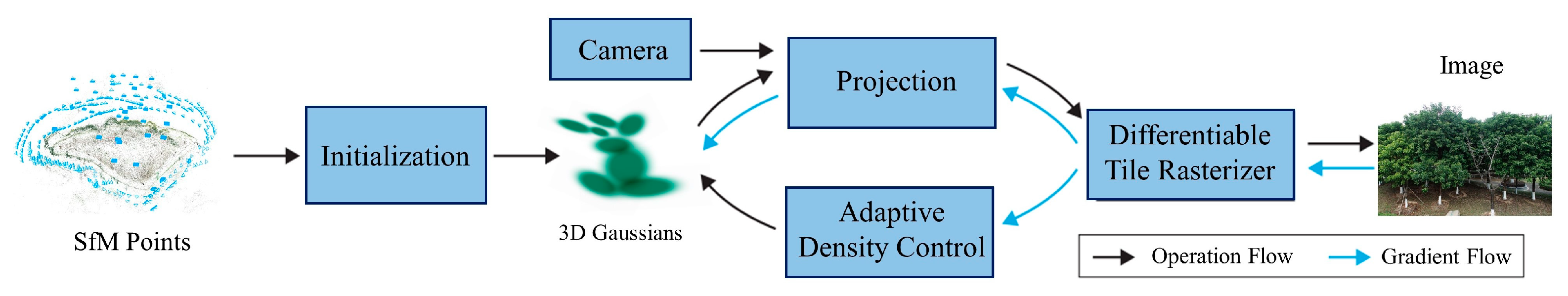
2.2.3. 3D Gaussian Splatting (3DGS)

3DGS defines the radiance field of a 3D scene as a discrete 3D Gaussian point cloud to achieve differentiable volume rendering. In 3DGS, each point is represented as an independent 3D Gaussian distribution, which is mathematically expressed as follows:

$$G\left(x\right)=\mathrm{e}\mathrm{x}\mathrm{p}(-{\displaystyle \frac{1}{2}}{(x-\mu )}^T{\Sigma }^{-1}\left(x-u\right))$$

(3)

where µ and Σ represent the mean and covariance matrix of the 3D Gaussian distribution, respectively. Each Gaussian point P is also assigned an opacity o and a color value c to represent the radiance field of the 3D scene.

Figure 2 shows an overview of the 3DGS rendering pipeline. The whole process can be divided into forward and backward stages. In the forward stage, based on the 3D Gaussian points and camera positions, the projections of the 3D Gaussian distributions and spherical harmonic functions onto the 2D plane are computed. Then, the Gaussian functions are overlaid and blended on the 2D plane, ultimately synthesizing the rendered image. In the backward phase, the loss is evaluated by calculating the difference between the rendered image and the real image, which is then used for backpropagation. The gradients from backpropagation are used to optimize the mean, covariance matrix, opacity, and spherical harmonic coefficients of the 3D Gaussian points. The loss function consists of a weighted sum of the minimum absolute deviation (L₁) and the structural similarity loss (L_D-SSIM), as follows:

$$L=\left(1-\lambda \right)L_1+\mathsf{\lambda }{L}_{D-SSIM}$$

(4)

In our forest stand reconstruction experiment, the original 3DGS algorithm was selected for testing. First, the sparse point cloud of the forest stand obtained from SfM was used as input to construct the initial 3D Gaussian point distribution, with each SfM point initialized as the center of a 3D Gaussian distribution. To improve the rendering quality, 3DGS introduced an adaptive density control mechanism, dynamically adjusting the number and distribution of Gaussian points through clone and split. The rendered scene was synthesized through training and exported in point cloud format, resulting in a 3D point cloud model of the forest stand.

2.3. Data Acquisition and Processing

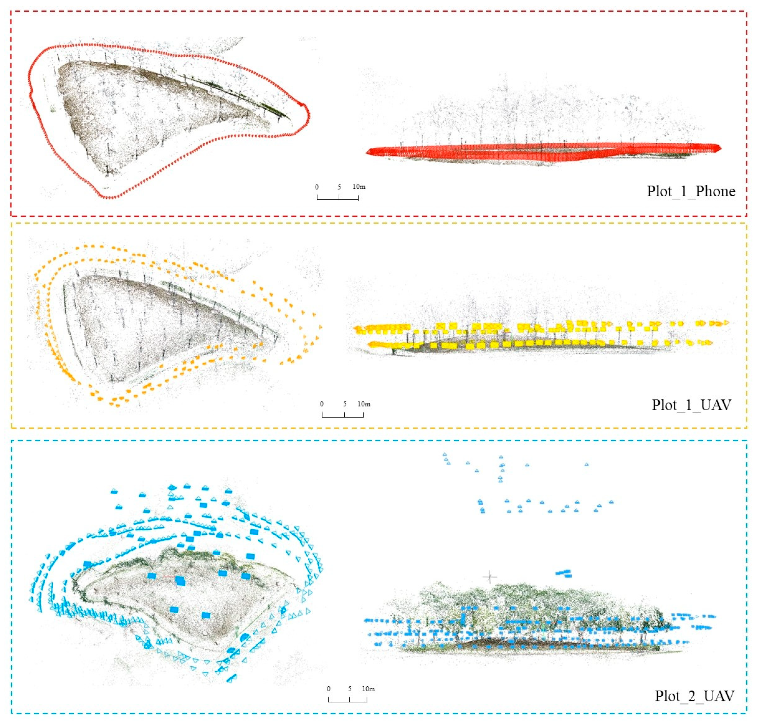
2.3.1. Data Acquisition

We used multiple devices and methods for data collection. An iPhone (Apple Inc., Cupertino, CA, USA) 11′s camera (12-megapixel, f/1.8) was used to capture 4K video footage of Plot_1 on the ground. Individual frames were then extracted from the video at a rate of 2 frames per second (fps), ensuring an overlap of over 70% between consecutive images. Additionally, a RGB camera (20-megapixel, f/2.8–f/11) on DJI Phantom 4 UAV (DJI, Shenzhen, China) was employed to manually collect image data of both Plot_1 and Plot_2. First, the UAV was hand-held to capture images at regular intervals while walking around the plots, followed by manual control of the UAV to capture aerial images above both plots. In both cases, an overlap of more than 70% was ensured between consecutive images. Figure 3 shows the camera positions for Plot_1 and Plot_2 obtained after being processed with COLMAP. These consumer-grade cameras are not only inexpensive but also easy to operate, and are widely used by the general public. The image resolution and number of images are detailed in

Table 1. Image data information for two forest stand plots.

Image Dataset	Number of Images	Image Resolution
Plot_1_Phone	279	3840 × 2160
Plot_1_UAV	268	5472 × 3648
Plot_2_UAV	322	5472 × 3648

Note: The first part of the image dataset type name represents the plot name, and the second part describes the image acquisition sensor, including a smartphone camera (Phone) and drone camera (UAV). For example, Plot_1_Phone refers to data collected on Plot_1 using a smartphone camera.

. The two plots were also scanned by a RIEGL VZ-400 (Riegl, Horn, Austria) terrestrial laser scanner (with the following parameters: accuracy of 3 mm, precision of 5 mm, laser beam divergence of 0.35 mrad, and angular resolution of 0.04 degrees). In order to obtain complete reference point cloud data, six scan stations were strategically placed around each plot to ensure maximal coverage. The point clouds from multiple scans were then coarsely and finely registered in the RiSCanPro software (Version 1.7.5), with a registration accuracy of approximately 4 mm. The Lidar point cloud data and image data for two plots were collected on the same day under clear and windless weather conditions.

2.3.2. Data Processing

The first step in photogrammetry, NeRF, and 3DGS reconstruction is the same SfM, which involves using the captured image data to obtain the corresponding camera poses and sparse point cloud. SfM results are used as input for MVS in photogrammetric processing. The entire photogrammetry reconstruction process is implemented using the open-source COLMAP. The NeRF method was implemented within the NeRFStudio, utilizing camera pose parameters and calibration images obtained from SfM for novel view synthesis and 3D model creation. The training process employed default parameters including the following: 30,000 iterations, a batch size of 4096 rays per training step, and a learning rate of 0.01. Once completed, the dense 3D point cloud model of the scene was exported. In the training of 3DGS, sparse point clouds obtained from SfM are used as initial values to construct an initial 3D Gaussian point cloud for rendering and optimization. Default training parameters included a learning rate of 0.01, 20,000 iterations, and a batch size of 1. In CloudCompare (Version 2.11), five non-tree feature markers were uniformly selected and registered with the TLS point cloud using the iterative closest point (ICP) algorithm, in order to assign real-world scale information to the dense point cloud models generated by photogrammetry, NeRF, and 3DGS. The registration accuracy ranged between 6 mm to 9 mm.

We next used LiDAR360 (Version 8.0) to perform preprocessing steps on the forest plot point cloud models. The processing included point cloud denoising using Gaussian filtering, followed by ground-vegetation separation through the cloth simulation filter (CSF) algorithm. The separated ground points were then utilized to normalize the vegetation points. Subsequently, for all forest stand point cloud models, we employed a distance-discriminant clustering method to automatically extract individual trees by setting identical threshold parameters, and acquired structural parameter information for each tree. We also conducted a comprehensive evaluation and analysis by visually and quantitatively comparing the distribution of and tree parameters extracted from different point cloud models. Figure 4 illustrates the workflow of this study. The cloud server system used for the reconstruction experiments (photogrammetry, NeRF, and 3DGS) was configured with Linux operating system, 12-core CPU, 24 GB RAM, NVIDIA GeForce RTX4090 (24 GB VRAM) GPU, deep learning framework of PyTorch 2.0 and CUDA 11.8.

3. Results

3.1. Reconstruction Efficiency Comparison

Since SfM is a common step among the three reconstruction methods, the MVS dense reconstruction process in photogrammetry is equivalent to the training process in NeRF and 3DGS. We will compare the time required for dense point cloud generation in COLMAP with the time required for training NeRF for 30,000 epochs and 3DGS for 20,000 epochs. In NeRF and 3DGS, training is typically completed after a fixed number of epochs. However, our preliminary observations indicate that the training loss of NeRF gradually converges and stabilizes after 25,000 epochs (with fluctuations of less than 0.1%), and no significant visual improvement is observed beyond that point. Similarly, the training loss of 3DGS usually stabilizes after 16,000 epochs (with fluctuations of less than 0.1%). Therefore, we believe that 30,000 epochs for NeRF and 20,000 epochs for 3DGS can achieve stable reconstruction results for model training in this scenario. As shown in

Table 2. Computation time (minutes) of dense reconstruction for different image datasets and dense reconstruction methods.

	Plot_1_Phone	Plot_1_UAV	Plot_2_UAV
COLMAP	544.292	724.495	453.834
NeRF	15.0	14.0	12.0
3DGS	18.23	17.39	17.46

, generally COLMAP requires the most time to generate dense point clouds, while NeRF requires the least amount of time. The time required for NeRF reconstruction ranges between 12–15 min, and the reconstruction time for 3DGS is approximately 1.3 times that of NeRF. In contrast, COLMAP is 37 to 51 times slower than the other two reconstruction methods. The total image resolution of the UAV dataset in Plot_1 is larger than that of the Phone dataset, so it took COLMAP more time for dense reconstruction. However, this was not the case for either NeRF or 3DGS; although Plot_2_UAV dataset is larger than Plot_1_UAV dataset, the processing times for COLMAP and NeRF are smaller instead. Overall, the time required for the two NVS reconstruction technologies is significantly less than that of the MVS dense reconstruction method in COLMAP.

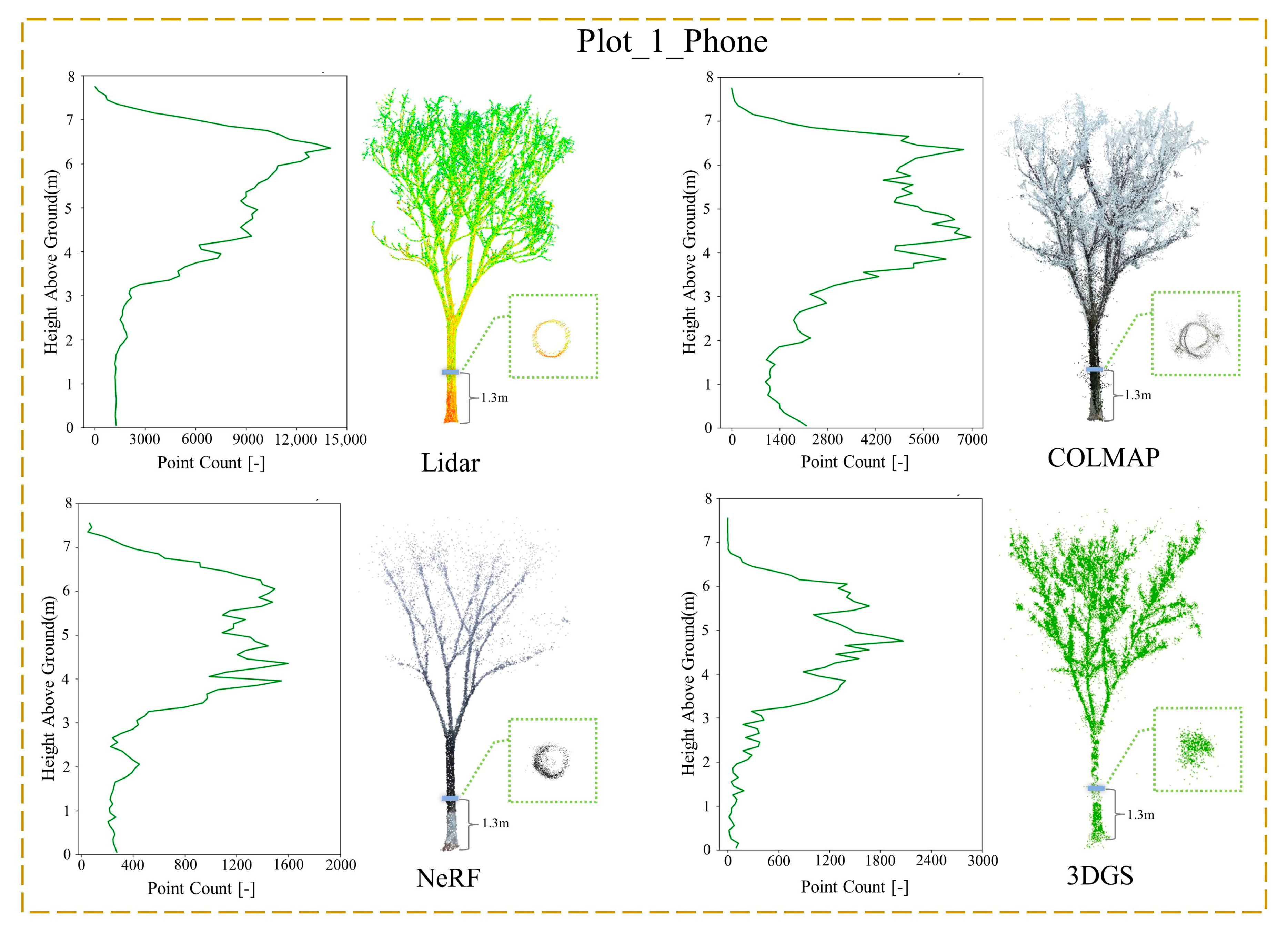
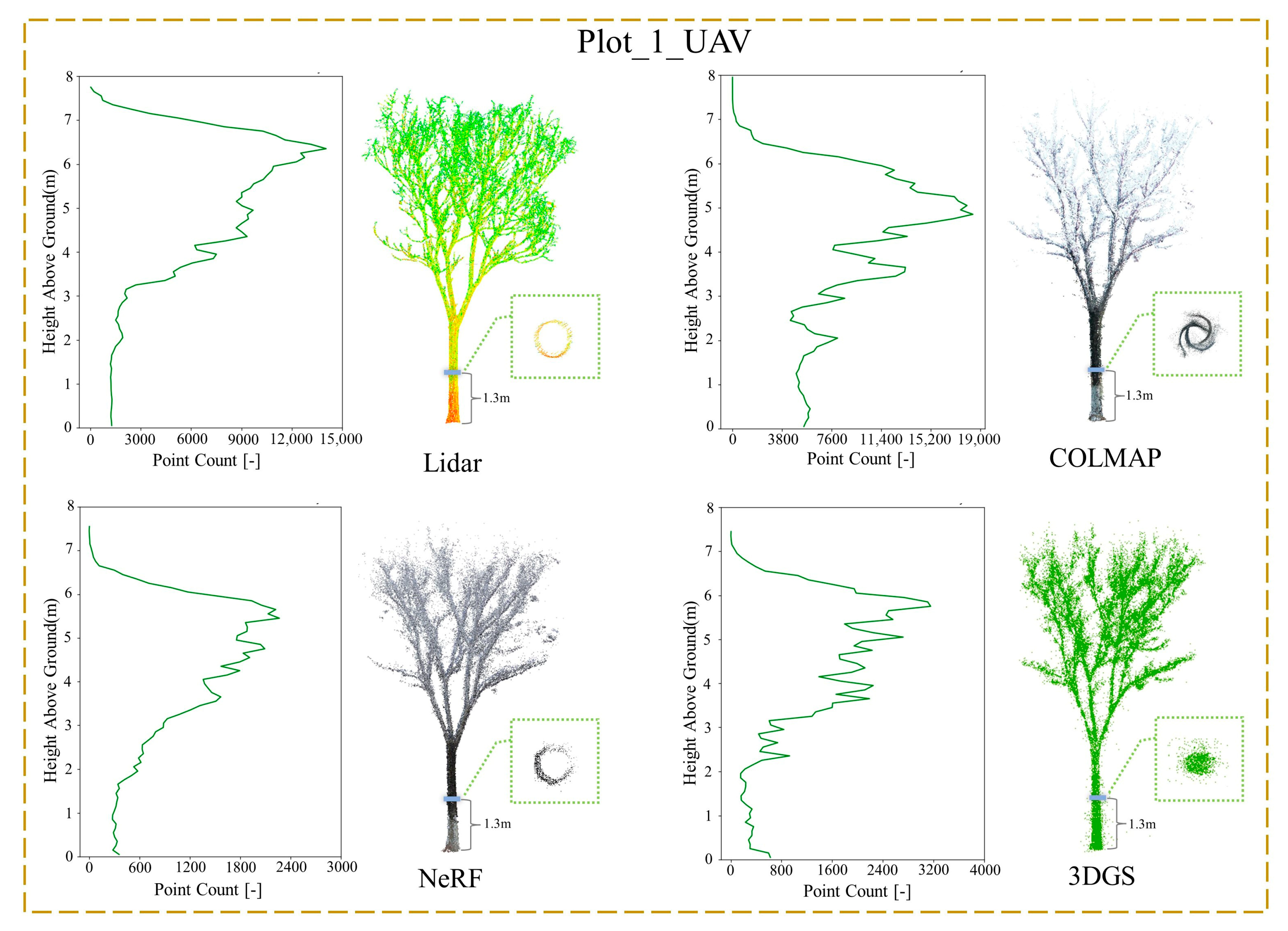
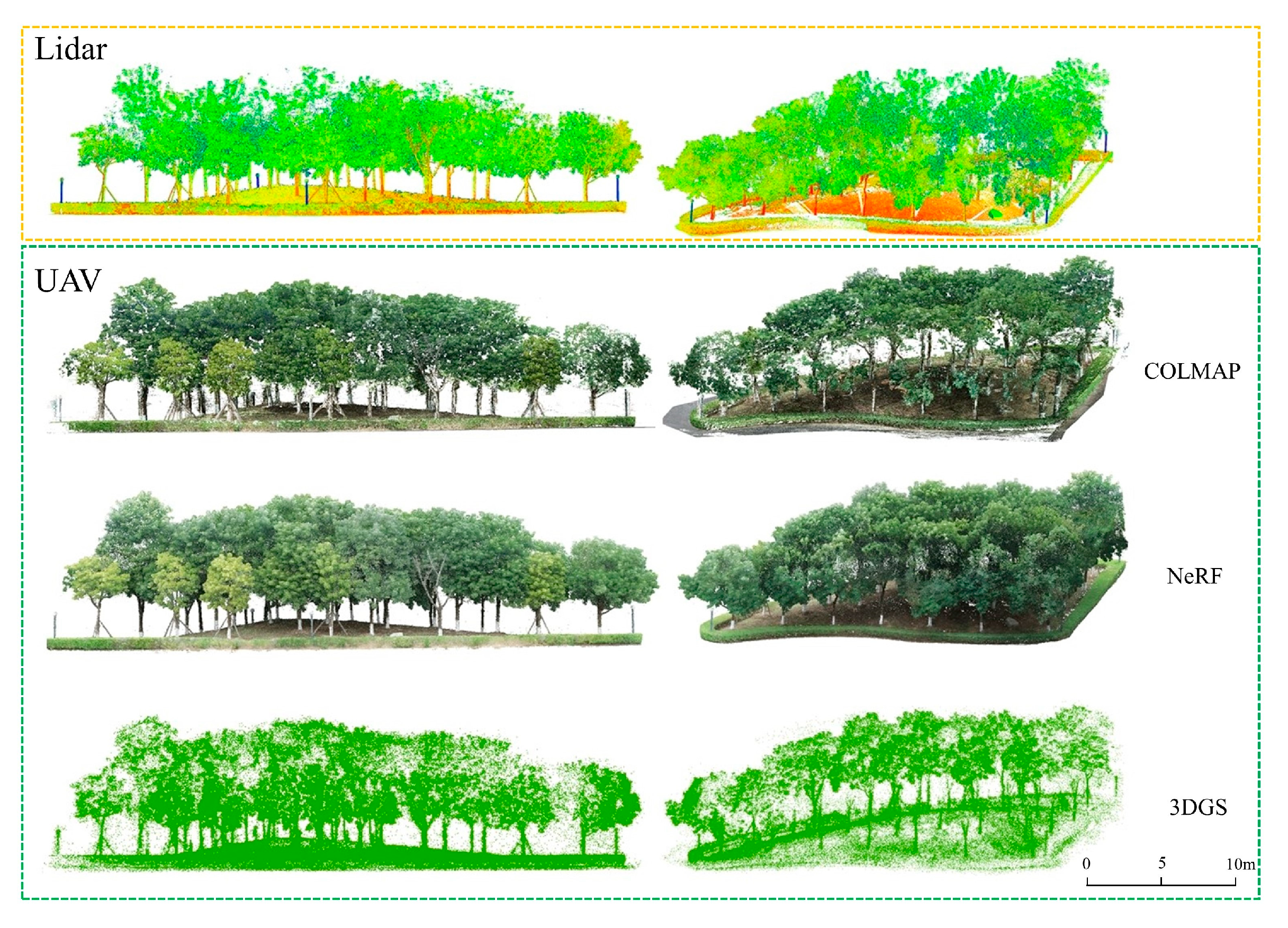
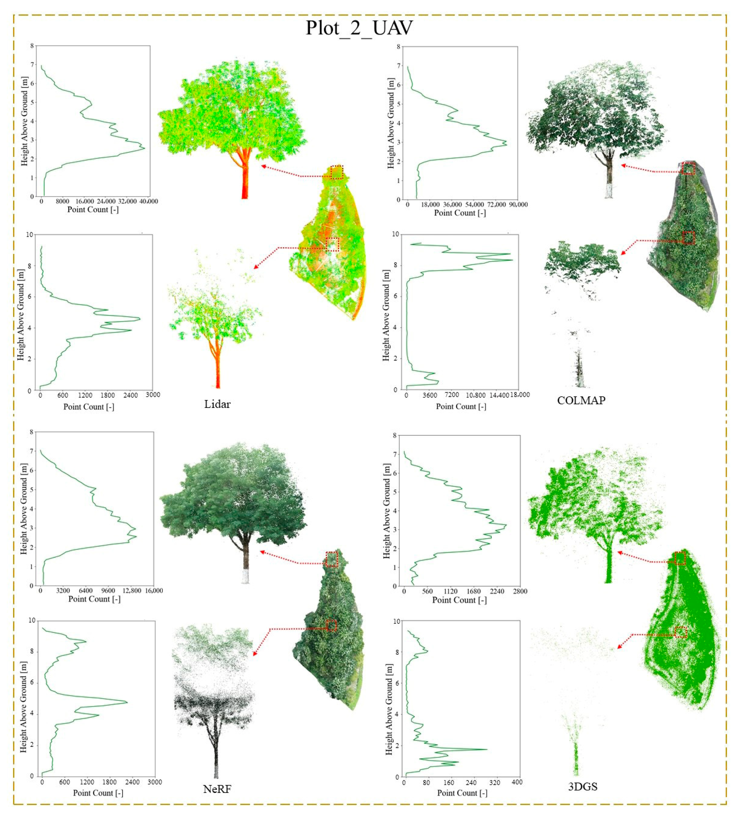
3.2. Point Cloud Comparison

We imported the point clouds obtained from COLMAP, NeRF, and 3DGS reconstructions into CloudCompare to register them with the laser scanned point cloud, and performed comparisons. The number of point clouds in the plot as obtained from various methods are summarized in

Table 3. Number of points in the tree point cloud models.

Plot ID	Model ID	Number of Points
Plot_1	Plot_1_Lidar	25,617,648
	Plot_1_Phone_COLMAP	20,200,476
	Plot_1_Phone_NeRF	4,548,307
	Plot_1_Phone_3DGS	1,555,984
	Plot_1_UAV_COLMAP	53,153,623
	Plot_1_UAV_NeRF	2,573,330
	Plot_1_UAV_3DGS	806,149
Plot_2	Plot_2_Lidar	9,053,897
	Plot_2_UAV_COLMAP	55,861,268
	Plot_2_UAV_NeRF	5,465,952
	Plot_2_UAV_3DGS	831,164

Note: The first part of the Model ID name indicates the name of the plot, the middle part describes the image acquisition sensor, which can be a smartphone camera (Phone) or an unmanned aerial vehicle (UAV), and the last part indicates the image reconstruction method, which can be COLMAP, 3DGS, or NeRF.

. Among the three reconstruction methods, COLMAP generates the most points, followed by NeRF, and 3DGS generates the fewest. The number of points generated by COLMAP is 4.4 to 20 times that of NeRF and 13 to 66 times that of 3DGS for the two plots. For COLMAP, more input pixel means higher number of output points; for NeRF and 3DGS, the relationships between input pixel and output point numbers are more nuanced and further investigation is needed.

Figure 5 shows the overall spatial distribution of point cloud for Plot_1, seeing from two distinct perspectives. Using Lidar as a reference model, the other three reconstruction methods successfully reconstruct Plot_1 visually. COLMAP and NeRF models contain color information, while 3DGS does not capture real-world color information and is therefore shown in green. The COLMAP model contains the most ground and trees and has the highest number of points, but it has more noise on the tree canopy and branches. Noise points in tree point clouds refer to those points that do not belong to the tree structure itself, such as those isolated or duplicate points. These noise points may be caused by sensor errors, environmental interference, image matching ambiguity, and other factors. Compared to the COLMAP model, the NeRF model contains fewer noise points, particularly in the UAV-based NeRF canopy. The 3DGS model has the fewest point clouds and appears sparser.

A single-tree model was selected from the point cloud model, and the vertical distribution of points was analyzed at 0.1 m intervals. Figure 6 and Figure 7, from left to right, show the vertical point distribution of the single-tree point cloud, the single-tree model, and a 10 cm thick trunk cross-section at a height of 1.3 m. Using the Lidar point cloud as a reference, its canopy region has a higher number of points, while the point distribution becomes smoother in the trunk region. In Plot_1_Phone, the three point clouds are generally similar to the Lidar distribution, but the COLMAP model exhibits significant fluctuations in the trunk region due to noise points, while the 3DGS model has fewer points in the trunk region. In Plot_1_UAV, the point distribution trend of NeRF aligns most closely with Lidar. Compared to the Phone dataset, the three tree point cloud models show an increased number of points in both the canopy and trunk regions. In the cross-sectional profiles of tree trunks, Lidar and NeRF models exhibit relatively smooth hollow circles, COLMAP model shows erroneous overlapping positions that increase the trunk diameter, and 3DGS model forms a solid circle with a smaller diameter.

Figure 8 displays the 3D reconstruction results of Plot_2, also from two different perspectives. The results indicate that the NeRF model is visually the best, achieving denser canopy 3D reconstruction with photorealistic color and minimal noise. Although the COLMAP model has the highest point density, there are missing areas in the canopy and some tree trunks. The 3DGS model is the sparsest, with more missing areas in the canopy and tree trunks compared to COLMAP and NeRF results.

To better compare the performance of different methods in reconstructing trees, two single-tree point cloud models were selected from Plot_2 to analyze the vertical distribution of points. One tree is located in the outer area, while the other is in the central area. Figure 9, from left to right, shows the vertical point distribution of the single-tree point cloud, the single-tree model, and the top-down view of the forest plot model. From the top-down view, it can be observed that the tree canopy in the middle of the Lidar model is incomplete, while the other three models successfully reconstructed the canopy. This is because the trees in Plot_2 are relatively tall, and the vertical scanning angle of TLS from the ground is limited (100 degrees), making it difficult to capture the upper parts of the canopy. Additionally, the dense leaves in the canopy block the laser beams, restricting their penetration. This is also evident in the vertical point distribution, where most of the points at the top of the canopy in the Lidar model are missing, with the point count approaching zero, especially for tree at the center. The other three models all have points at the top of the canopy, though the 3DGS model shows a relatively sparse distribution. NeRF has fewer points in the middle of the canopy (around 6 m) but reconstructs more details in the trunk and branches, making it the closest to the Lidar model. Both COLMAP (2–7 m) and 3DGS (4–7 m) exhibit missing points in the middle of the trunk and canopy, but 3DGS has fewer points in the trunk region. For the tree model in the peripheral area, the Lidar model achieves a complete reconstruction. Using Lidar as a reference, NeRF produces the best results, with a complete and dense canopy and trunk, and both Lidar and NeRF show a clear inflection point at around 1.3 m in their vertical distribution of points. In contrast, the COLMAP model has sparser canopy points. Additionally, in the vertical distribution, a clear inflection point appears at 2 m, indicating missing parts in the trunk. The 3DGS model has sparse canopy points and significant fluctuations in its vertical point distribution.

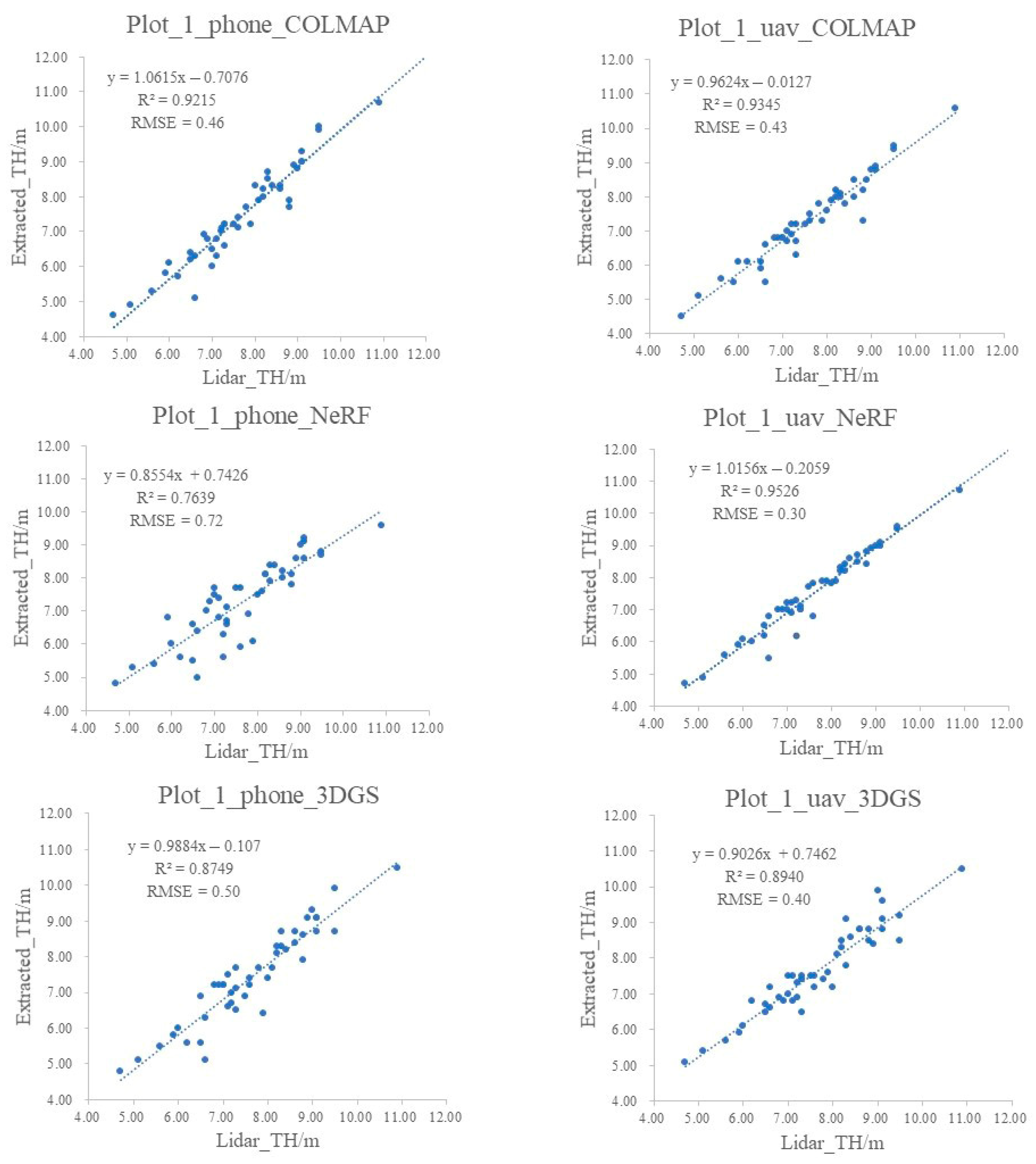
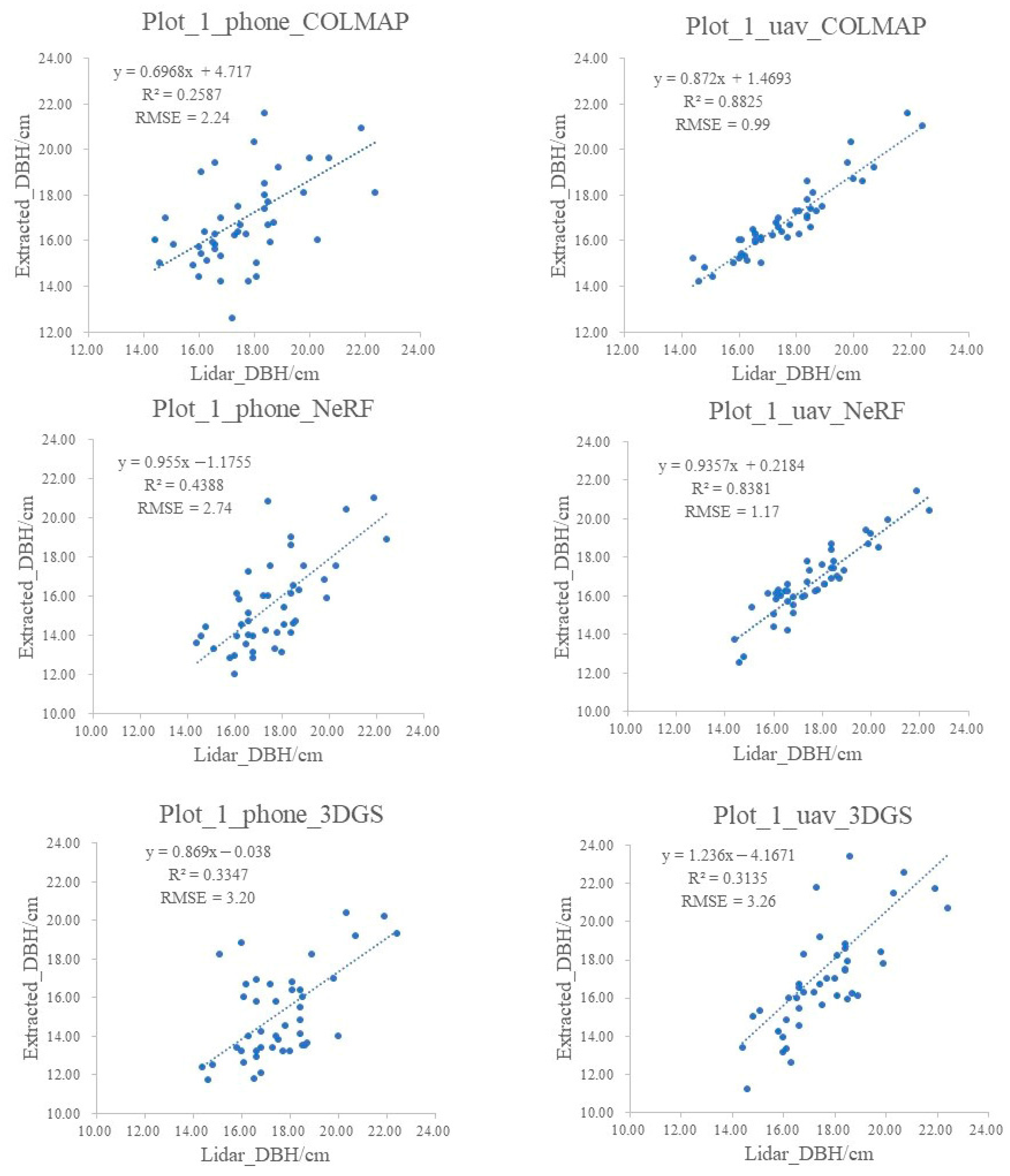
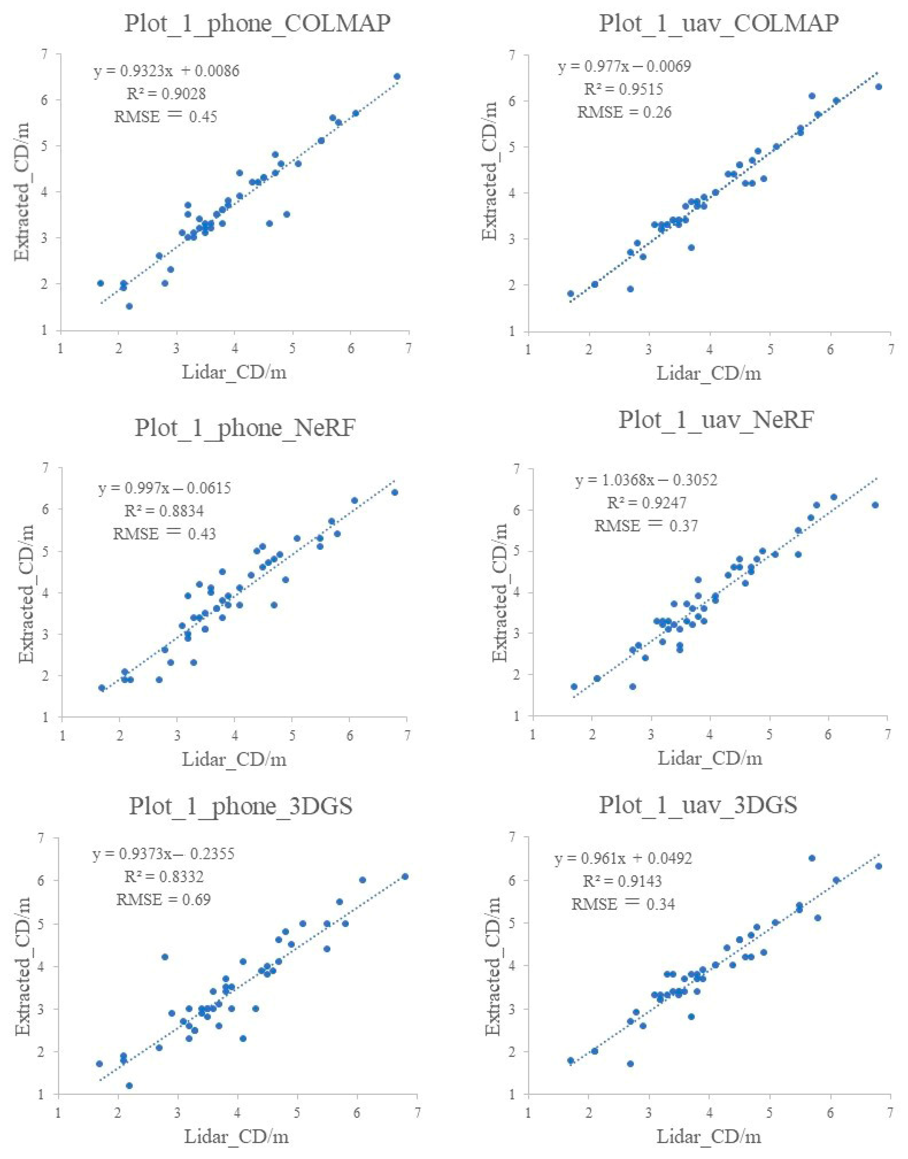
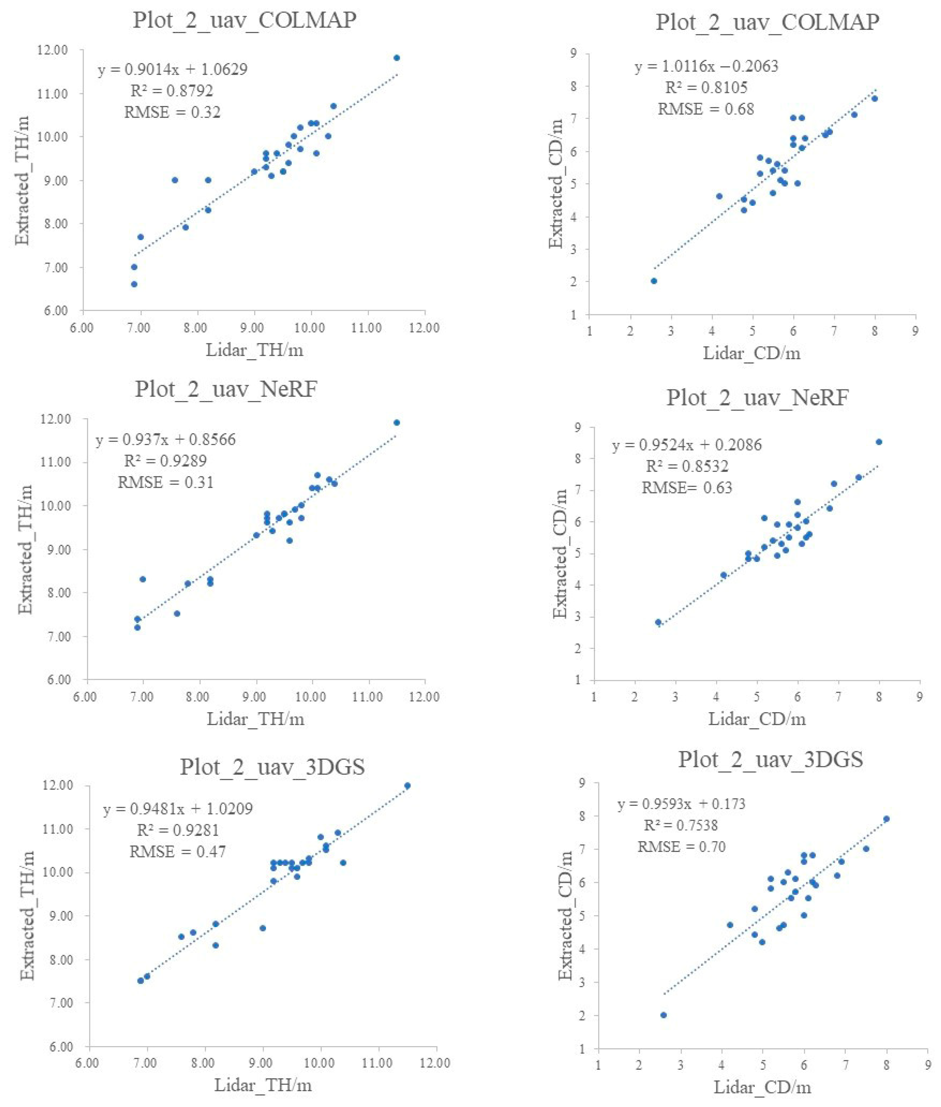
3.3. Extraction of Tree Parameters from Stand Plot Point Cloud

Using the same procedure and parameters in LiDAR360, individual trees were automatically segmented for all the point cloud models. In Plot_1, all three models correctly segmented 45 trees. However, in the more complex Plot_2, COLMAP segmented 38 trees, incorrectly over-segmenting 5 additional trees, while NeRF and 3DGS both correctly extracted 33 trees. Additionally, we obtained the TH, DBH, and CD for each tree in the plot and conducted a quantitative comparison of the tree parameters among the three visual reconstruction models, using the data from the Lidar model as a reference. However, due to the taller trees and denser canopy in Plot_2, a small portion of canopy points in the center of the plot were missing in the LiDAR data, which introduces certain limitations for using TH and CD from the LiDAR model as reference values.

The coefficient of determination (R²) and root mean square error (RMSE) were used as evaluation metrics for the structural parameters. The R² value assesses how well the regression model fits the reference data, with a value closer to 1 indicating a higher correlation between the data and a more accurate description of the variations. RMSE represents the average deviation between the true values of the structural parameters and the observed values. In forest resource surveys, an R² greater than 0.8 indicates good fitting performance. Using TLS survey accuracy as the reference standard, the required precision ranges for various parameters are DBH (0–2 cm), TH (0–0.5 m), and CD (0.5–1 m) [9].

$$R^2=1-{\displaystyle \frac{{\sum }_{i=1}^m{\left(y_i-{\widehat{y}}_i\right)}^2}{{\sum }_{i=1}^m{\left(y_i-\overline{y}\right)}^2}}$$

(5)

$$RMSE=\sqrt{{\displaystyle \frac{1}{m}}{\sum }_{i=1}^m{\left(y_i-{\widehat{y}}_i\right)}^2}$$

(6)

where ${\widehat{y}}_i$ and $y_i$ represent the predicted and observed values of the samples, respectively, $\overline{y}$ denotes the mean of the observed values, and m is the number of samples.

Figure 10 and Figure 11 display the results of linear fitting between the TH and DBH extracted from three models and the Lidar reference values for Plot_1. For three THs, Phone_COLMAP and Phone_3DGS show good fitting with Lidar, with R² of 0.9215 and 0.8749, and RMSE values of 0.46 m and 0.50 m, respectively. Phone_NeRF suffers from a misalignment of ground and tree trunk points, which affects the accuracy of TH extraction, resulting in an R² of 0.7639 and an RMSE of 0.71 m. The three models reconstructed from UAV imagery improve the accuracy of TH extraction, with R² values of 0.9345, 0.8940, and 0.9526 for COLMAP, 3DGS, and NeRF, respectively, representing improvements of 1.60%, 1.91%, and 18.87% compared to the Phone models. RMSE values also decrease to 0.43 m, 0.40 m, and 0.29 m, respectively.

In the DBH extractions for Plot_1, none of the three point cloud models from Phone achieved a good fit for DBH, with R² values all below 0.5, where Phone_NeRF has the best fit at 0.4388. The UAV_COLMAP and UAV_NeRF models are closer to Lidar values compared to those of Phone models, with R² values of 0.8825 and 0.8381, representing increases of 62.41% and 39.93%, respectively. The RMSE values have also decreased to 0.99 cm and 1.17 cm. The Phone_3DGS and UAV_3DGS models show much smaller DBH values than the Lidar reference due to the sparse nature of the tree trunks in these models.

Figure 12 shows the crown diameter extraction results of the Plot_1 model. The linear fits of each model are relatively good, among which uav_COLMAP achieves the highest R² value of 0.9515 and an RMSE of 0.26, while the lowest is phone_3DGS with an R² value of 0.8332 and an RMSE of 0.69. Similarly, the UAV models exhibit better fits compared to the Phone models, with the R² increasing by 0.041–0.081 and the RMSE decreasing by 0.06 m–0.35 m.

Figure 13 shows the linear fitting results of TH and CD extracted from models compared to those derived from Lidar reference values for Plot_2. The left column of the figure represents TH, while the right column represents CD. In the extraction of these two parameters, the central trees were excluded for comparison due to the fact that the Plot_2_Lidar model is missing some canopy information. For TH extraction, COLMAP’s R² reached 0.8792, with an RMSE of 0.32 m. 3DGS and NeRF models have R² values of 0.9289 and 0.9281, with RMSE of 0.47 m and 0.31 m, respectively, indicating that their extracted TH values are closer to Lidar TH values when compared to COLMAP. For CD extraction, COLMAP and NeRF both achieved R² values exceeding 0.8, with 0.8105 and 0.8532, respectively, and RMSE values of 0.68 and 0.63. 3DGS performed the worst, with R² of 0.7538 and RMSE of 0.70. Compared to the TH and CD parameters in Plot_1, both R² and RMSE values deteriorated in Plot_2 due to increased canopy occlusion and complexity. The R² values decreased by a range of 0.024 to 0.160, while the RMSE values increased by 0.01 m to 0.36 m.

Figure 14 shows the DBH extraction results of the Plot_2_UAV model. Due to the sparse distribution of tree trunk points in the Plot_2_UAV_3DGS model, DBH fitting could not be performed, and some reconstructed tree trunks did not reach the required height for DBH (1.3 m). Therefore, DBH values could not be successfully extracted. The DBH values obtained from COLMAP and NeRF with R² values of 0.8747 and 0.8648, and RMSE values of 1.60 cm and 1.63 cm, respectively.

4. Discussion

In this study, we applied three image-based 3D reconstruction techniques in forest stands, including a photogrammetry pipeline (SfM + MVS in COLMAP) and novel view synthesis-based methods (NeRF and 3DGS). By comparing the dense point cloud models generated by these three methods with the reference TLS point clouds, we analyzed the reconstruction efficiency and point cloud model quality of different methods for reconstructing forest stands.

The difficulty in successfully reconstructing multi-view 3D models of forest stands typically lies in the fact that trees of the same species have similar texture structures, making it challenging for algorithms to distinguish (detect and match) tree features. Additionally, due to the occlusion of tree branches and canopies, the views could change dramatically even between two adjacent images. The first step for photogrammetry, NeRF, and 3DGS is to obtain accurate camera poses and calibrated images through SfM. If the results of SfM are inaccurate, it will affect the subsequent dense reconstruction outcomes, for example, duplicated (phantom) trunks can appear at the same location with a small offset. In the COLMAP pipeline, the steps of SfM include feature extraction, feature matching, and triangulation of points. During our SfM experiments, we found that the results of feature matching are related to the completeness of the camera pose estimation. By default, COLMAP uses exhaustive matching (where all images are matched pairwise). Using this method for matching the images of Plot_1_UAV and Plot_2_UAV, SfM was only able to successfully solve for the poses of 173 images (out of total input of 268 images) and 268 images (input of 322 images), respectively, along with generating a sparse point cloud for parts of the scene. However, COLMAP also supports other matching methods, such as spatial matching (which requires images to have positional information, such as GPS data). Considering that the UAV images of Plot_1 and Plot_2 contain positioning information, using spatial matching allows for the successful retrieval of the complete camera pose information for all input images (Plot_1_UAV: 268 images, Plot_2_UAV: 322 images) and a more complete feature point cloud. The results of downstream dense reconstruction (MVS, NVS) depend to a large extent on the accuracy of the upstream SfM results, which is why spatially matched SfM results are used during the dense reconstruction phase. To reduce dependence on SfM, some studies have utilized optical flow and point trajectory principles for camera pose estimation [46]. Others have integrated the camera pose estimation step into the 3DGS network training framework, simultaneously optimizing both 3DGS and camera poses [47]. Additionally, the scene regression-based ACE0 [48] method and the general-purpose global SfM method GLOMAP [49] significantly improve operational efficiency and achieve SfM estimates comparable to COLMAP. More robust feature matching methods, such as LoFTR [50] and RCM [51], can also replace the feature matching step in SfM to improve matching accuracy.

MVS utilizes the corresponding images and camera parameters obtained from sparse reconstruction to reconstruct a dense point cloud model through multi-view stereopsis. This process involves calculating depth information for each image and fusing depth maps. Typically, the time required to compute depth information occupies the majority of the MVS dense reconstruction time. Moreover, the time consumption increases with the size, complexity of the scene, and the number of images. In a previous study on single tree reconstruction, the MVS dense reconstruction of a single tree (with 107–237 input images) usually took 50 to 100 min on a single 3090 GPU [38]. However, in this study, despite using the more computationally efficient 4090 GPU, the reconstruction of forest plot scenes (with 268–322 input images) still took 450 to 700 min. The average processing time per input image increases from 0.43–0.83 min to 1.40–2.70 min, an approximate increase of about 3.3 times. But the COLMAP processing time for Plot_2_UAV (more images and higher total resolution) was shorter than that for Plot_1_UAV. This may be because the scene in Plot_1 was relatively simpler and had clearer textures, which led to a larger number of detectable feature points, thereby increasing the time required for reconstruction. The efficiency of reconstruction is influenced by multiple factors, and further experiments and analysis are needed to better understand these effects. In contrast, efficient deep learning networks like NeRF and 3DGS can significantly reduce the reconstruction time, usually completing within 20 min, and the time required appears to be independent of the scene size and the number of images.

By comparing the number of points, overall view, and detailed vertical profiles of the point cloud tree models, we highlight the advantages and disadvantages of the three image-based reconstruction methods. The COLMAP method can generate models with the highest number of points, but it tends to introduce more noise in the trunk and canopy layers. Comparing the COLMAP models of Plot_1_Phone and Plot_1_UAV, the UAV provides more image data for the canopy, which reduces noise in the UAV_COLMAP model’s canopy region. However, a significant amount of noise remains. In contrast, the NeRF model exhibits less noise in the canopy. When there is ground occlusion or limited viewpoints, such as in the case of Plot_1_Phone, the NeRF model exhibits missing or erroneous reconstructions in the ground regions. The 3DGS model contains the fewest points, with fewer than 2 million points overall, resulting in a sparse and low-quality point cloud model that fails to represent real-world accurately. This indicates that the ability of 3DGS to generate dense point cloud models is inferior to that of COLMAP and NeRF. In the more complex scene of Plot_2, NeRF can produce point cloud models closest to those obtained from Lidar, compared to COLMAP and 3DGS models. NeRF reconstructs colored and more detailed trunks, and captures more complete canopies. This advantage may be attributed to NeRF’s differentiable implicit volumetric representation, which optimizes camera poses through backpropagated loss gradients. This approach significantly reduces pose estimation errors even with imperfect input data, thereby enhancing scene clarity and detail representation to achieve high-quality reconstruction. Meanwhile, the COLMAP model occasionally shows intersecting trunks or multiple overlapping trees. These observations demonstrate that NeRF is better suited to handling complex forest stand, but requires complete viewing angle coverage during data acquisition.

When selecting plots and collecting data, different types of plots and data acquisition methods were chosen with the aim of comparing and illustrating how these factors might affect the results. We selected two plots with different tree species and canopy morphologies: Plot_1 consisted of leafless trees with simple branch structures and less occlusion between trees, resulting in more complete tree point cloud models reconstructed by all three methods. In contrast, Plot_2 has dense foliage and more occlusions, which led to incomplete tree trunks and missing canopies in the middle of the plot. However, compared to the other two methods, NeRF was better able to handle occluded scenes, producing tree point cloud models with more detailed trunk structures and more complete canopies. For Plot_1, image data were collected using both a smartphone (capturing lower-resolution images from the ground only) and a UAV (capturing higher-resolution images from both ground and aerial perspectives). The UAV images, which provided more viewpoints, resulted in more complete tree point cloud models with fewer noise points in the canopy. Furthermore, models generated from higher-resolution images contained more detailed tree features. The quality of the models also significantly impacted the accuracy of subsequent individual tree structure parameter extraction. For example, the tree crown diameter extracted by the UAV model in Plot_1 is more accurate than that by the phone, with R² increasing by 0.041–0.081 and RMSE decreasing by 0.06 m–0.35 m.

We performed individual tree segmentation on different point cloud models and extracted TH, DBH, and CD as individual tree structural parameters for comparison. During the individual tree segmentation process, the number of trees in the Plot_2_COLMAP model exceeded the actual count. This could be attributed to the high similarity in texture features and partial occlusion among trees in this plot, which reduces the number of feature points and results in mismatches, causing a single tree to be represented by multiple duplicated models. Therefore, the conventional photogrammetry algorithm (SfM + MVS) sometimes is unable to handle more complex forest plot scenes. In terms of TH parameters, all three methods achieve high accuracy in terms of RMSE and R², with estimates from the NeRF model generally outperforming those from the COLMAP and 3DGS models. In terms of DBH estimation, the models generated from lower-resolution smartphone images show poorer accuracy, while the models reconstructed from higher-resolution UAV images demonstrate higher precision. Among them, the COLMAP model provides better DBH estimates; however, in the extracted individual COLMAP tree models, some phantom tree trunks often intersect each other, which may cause the estimated DBH values to be larger than the actual ones. The NeRF method has slightly lower estimation accuracy compared to the photogrammetry approach and tends to underestimate the DBH values. The 3DGS method yields the least accurate DBH estimates, as its reconstructed points are relatively sparse and trunk points tend to cluster together, leading to DBH estimates that are significantly lower than the reference Lidar DBH values. In terms of the crown width parameter, for the simple canopies in Plot_1, all three methods achieve relatively accurate crown diameters, with UAV models showing higher R² values than Phone models, indicating that images collected by drones result in more complete tree canopies during reconstruction. Compared to Plot_1, the denser canopy in Plot_2 shows that COLMAP and NeRF produce denser canopy point clouds, while 3DGS has sparser canopies and lower R² values for crown diameter. The above results indicate that photogrammetry can provide more accurate DBH estimations in relatively simple forest plots, though it yields lower-quality tree point clouds. In contrast, NeRF achieves higher-quality point cloud reconstructions, and thus more accurate estimations of TH and CD. These findings also demonstrate that higher-resolution and more comprehensive UAV imagery can enhance the quality of reconstructed tree point clouds and improve the accuracy of structural parameter extraction.

We acknowledge that this research is limited in scope, as the current study was conducted in only two small plots with homogeneous tree species and limited terrain variation. However, our findings suggest that NeRF holds greater potential than photogrammetry for applications in complex forest environments. Therefore, future studies will expand the scope to include larger and more complex forest plots. Additionally, when extending this approach to other forest scenarios, attention should be paid to the resolution of the collected images, and careful planning of data acquisition routes is necessary to ensure the complete image coverage of the study area.

Through this study, we have gained a deeper understanding of the practical applications of NeRF and 3DGS methods in forest scenes and the properties of the dense point cloud data generated by these methods, provided answers to the questions raised in the introduction earlier. At the same time, we outline prospects for future research: how to improve the accuracy of sparse point clouds and camera pose parameters obtained from upstream SfM, potentially by using more robust feature matching techniques and alternative SfM solutions, and by enhancing feature matching success rates through image enhancement methods; and how to enhance the ability of NeRF and 3DGS to generate dense point clouds. Equipping NVS technology into lightweight devices (such as smartphones and drones) through dedicated applications to achieve real-time, online 3D tree reconstruction and structural parameter acquisition is also one of our goals. We expect the emergence of more powerful software tools and carefully designed strategies that will enable efficient and highly accurate 3D reconstruction of forest scenes, providing convenience for urban tree management.

5. Conclusions

This study applied NVS (NeRF and 3DGS) techniques to the 3D dense reconstruction of urban forest stands. Using two forest plots with different tree structures and morphologies (one leaf-on and one leaf-off) as examples, the feasibility of these techniques was tested. Specifically, dense point cloud models were generated using NVS techniques based on sequential images captured from different devices and viewpoints, and were compared with photogrammetric methods. A comprehensive evaluation of the practical application of different NVS methods in forest stand was conducted in terms of processing efficiency, point cloud model quality, and the accuracy of tree parameters extraction. The results demonstrated that the following:

• The new view synthesis methods (NeRF and 3DGS) achieve significantly higher efficiency in dense reconstruction compared to classic photogrammetry methods;
• The 3DGS method’s capability to generate dense 3D point clouds is inferior to that of NeRF and photogrammetry methods, with 3DGS models often exhibiting sparser point densities and being inadequate for single-tree diameter estimation;
• For forest stands with dense foliage, NeRF provides superior reconstruction quality, while photogrammetry methods tend to produce poorer results, including issues such as tree trunk overlap and multiple tree duplications;
• All three methods achieve high accuracy in extracting single-tree height and crown diameter parameters, with NeRF providing the highest precision for tree height. Photogrammetry methods offer better accuracy in diameter estimation compared to NeRF and 3DGS;
• Image resolution and the completeness of viewpoints also impact the quality of the reconstruction results and the accuracy of tree structure parameter extraction.

References

1. Baumeister, C.F.; Gerstenberg, T.; Plieninger, T.; Schraml, U. Exploring cultural ecosystem service hotspots: Linking multiple urban forest features with public participation mapping data. Urban For. Urban Green. 2020, 48, 126561. [Google Scholar] [CrossRef]
2. Escobedo, F.J.; Nowak, D. Spatial heterogeneity and air pollution removal by an urban forest. Landsc. Urban Plan. 2009, 90, 102–110. [Google Scholar] [CrossRef]
3. Zhang, B.; Li, X.; Du, H.; Zhou, G.; Mao, F.; Huang, Z.; Zhou, L.; Xuan, J.; Gong, Y.; Chen, C. Estimation of urban forest characteristic parameters using UAV-Lidar coupled with canopy volume. Remote Sens. 2022, 14, 6375. [Google Scholar] [CrossRef]
4. Lin, J.; Chen, D.; Wu, W.; Liao, X. Estimating aboveground biomass of urban forest trees with dual-source UAV acquired point clouds. Urban For. Urban Green. 2022, 69, 127521. [Google Scholar] [CrossRef]
5. Isibue, E.W.; Pingel, T.J. Unmanned aerial vehicle based measurement of urban forests. Urban For. Urban Green. 2020, 48, 126574. [Google Scholar] [CrossRef]
6. Çakir, G.Y.; Post, C.J.; Mikhailova, E.A.; Schlautman, M.A. 3D LiDAR scanning of urban forest structure using a consumer tablet. Urban Sci. 2021, 5, 88. [Google Scholar] [CrossRef]
7. Bobrowski, R.; Winczek, M.; Zięba-Kulawik, K.; Wężyk, P. Best practices to use the iPad Pro LiDAR for some procedures of data acquisition in the urban forest. Urban For. Urban Green. 2023, 79, 127815. [Google Scholar] [CrossRef]
8. Luoma, V.; Saarinen, N.; Wulder, M.A.; White, J.C.; Vastaranta, M.; Holopainen, M.; Hyyppä, J. Assessing precision in conventional field measurements of individual tree attributes. Forests 2017, 8, 38. [Google Scholar] [CrossRef]
9. Liang, X.; Kankare, V.; Hyyppä, J.; Wang, Y.; Kukko, A.; Haggrén, H.; Yu, X.; Kaartinen, H.; Jaakkola, A.; Guan, F. Terrestrial laser scanning in forest inventories. ISPRS J. Photogramm. Remote Sens. 2016, 115, 63–77. [Google Scholar] [CrossRef]
10. Chen, C.; Wang, H.; Wang, D.; Wang, D. Towards the digital twin of urban forest: 3D modeling and parameterization of large-scale urban trees from close-range laser scanning. Int. J. Appl. Earth Obs. Geoinf. 2024, 127, 103695. [Google Scholar] [CrossRef]
11. Holopainen, M.; Kankare, V.; Vastaranta, M.; Liang, X.; Lin, Y.; Vaaja, M.; Yu, X.; Hyyppä, J.; Hyyppä, H.; Kaartinen, H. Tree mapping using airborne, terrestrial and mobile laser scanning–A case study in a heterogeneous urban forest. Urban For. Urban Green. 2013, 12, 546–553. [Google Scholar] [CrossRef]
12. D’hont, B.; Calders, K.; Bartholomeus, H.; Lau, A.; Terryn, L.; Verhelst, T.; Verbeeck, H. Evaluating airborne, mobile and terrestrial laser scanning for urban tree inventories: A case study in Ghent, Belgium. Urban For. Urban Green. 2024, 99, 128428. [Google Scholar] [CrossRef]
13. Dos Santos, R.C.; Da Silva, M.F.; Tommaselli, A.M.G.; Galo, M. Automatic Tree Detection/Localization in Urban Forest Using Terrestrial Lidar Data. In Proceedings of the IGARSS 2024-2024 IEEE International Geoscience and Remote Sensing Symposium, Athens, Greece, 7–12 July 2024; pp. 4522–4525. [Google Scholar]
14. Reddy, S.; Fararoda, R.; Jha, C.S.; Rajan, K.S. Automatic estimation of tree stem attributes using terrestrial laser scanning in central Indian dry deciduous forests. Curr. Sci. 2018, 114, 201–206. [Google Scholar] [CrossRef]
15. Magnuson, R.; Erfanifard, Y.; Kulicki, M.; Gasica, T.A.; Tangwa, E.; Mielcarek, M.; Stereńczak, K. Mobile Devices in Forest Mensuration: A Review of Technologies and Methods in Single Tree Measurements. Remote Sens. 2024, 16, 3570. [Google Scholar] [CrossRef]
16. Liang, X.; Hyyppä, J.; Kaartinen, H.; Lehtomäki, M.; Pyörälä, J.; Pfeifer, N.; Holopainen, M.; Brolly, G.; Francesco, P.; Hackenberg, J. International benchmarking of terrestrial laser scanning approaches for forest inventories. ISPRS J. Photogramm. Remote Sens. 2018, 144, 137–179. [Google Scholar] [CrossRef]
17. Jaskierniak, D.; Lucieer, A.; Kuczera, G.; Turner, D.; Lane, P.; Benyon, R.; Haydon, S. Individual tree detection and crown delineation from Unmanned Aircraft System (UAS) LiDAR in structurally complex mixed species eucalypt forests. ISPRS J. Photogramm. Remote Sens. 2021, 171, 171–187. [Google Scholar] [CrossRef]
18. Liao, K.; Li, Y.; Zou, B.; Li, D.; Lu, D. Examining the role of UAV Lidar data in improving tree volume calculation accuracy. Remote Sens. 2022, 14, 4410. [Google Scholar] [CrossRef]
19. Sadeghian, H.; Naghavi, H.; Maleknia, R.; Soosani, J.; Pfeifer, N. Estimating the attributes of urban trees using terrestrial photogrammetry. Environ. Monit. Assess. 2022, 194, 625. [Google Scholar] [CrossRef]
20. Zhang, Z.; Yun, T.; Liang, F.; Li, W.; Zhang, T.; Sun, Y. Study of Obtain of Key Parameters of Forest Stand Based on Close Range Photogrammetry. Sci. Technol. Eng 2017, 17, 85–92. [Google Scholar]
21. Roberts, J.; Koeser, A.; Abd-Elrahman, A.; Wilkinson, B.; Hansen, G.; Landry, S.; Perez, A. Mobile terrestrial photogrammetry for street tree mapping and measurements. Forests 2019, 10, 701. [Google Scholar] [CrossRef]
22. Shao, T.; Qu, Y.; Du, J. A low-cost integrated sensor for measuring tree diameter at breast height (DBH). Comput. Electron. Agric. 2022, 199, 107140. [Google Scholar] [CrossRef]
23. Schonberger, J.L.; Frahm, J.-M. Structure-from-motion revisited. In Proceedings of the IEEE Conference on Computer Vision and Pattern Recognition, Las Vegas, NV, USA, 27–30 June 2016; pp. 4104–4113. [Google Scholar]
24. Seitz, S.M.; Curless, B.; Diebel, J.; Scharstein, D.; Szeliski, R. A comparison and evaluation of multi-view stereo reconstruction algorithms. In Proceedings of the 2006 IEEE Computer Society Conference on Computer Vision and Pattern Recognition (CVPR’06), New York, NY, USA, 17–22 June 2006; pp. 519–528. [Google Scholar]
25. Kameyama, S.; Sugiura, K. Estimating Tree Height and Volume Using Unmanned Aerial Vehicle Photography and SfM Technology, with Verification of Result Accuracy. Drones 2020, 4, 19. [Google Scholar] [CrossRef]
26. Bayati, H.; Najafi, A.; Vahidi, J.; Gholamali Jalali, S. 3D reconstruction of uneven-aged forest in single tree scale using digital camera and SfM-MVS technique. Scand. J. For. Res. 2021, 36, 210–220. [Google Scholar] [CrossRef]
27. Xu, Z.; Shen, X.; Cao, L. Extraction of Forest Structural Parameters by the Comparison of Structure from Motion (SfM) and Backpack Laser Scanning (BLS) Point Clouds. Remote Sens. 2023, 15, 2144. [Google Scholar] [CrossRef]
28. Zhu, R.; Guo, Z.; Zhang, X. Forest 3D reconstruction and individual tree parameter extraction combining close-range photo enhancement and feature matching. Remote Sens. 2021, 13, 1633. [Google Scholar] [CrossRef]
29. Mildenhall, B.; Srinivasan, P.P.; Tancik, M.; Barron, J.T.; Ramamoorthi, R.; Ng, R. Nerf: Representing scenes as neural radiance fields for view synthesis. Commun. ACM 2021, 65, 99–106. [Google Scholar] [CrossRef]
30. Müller, T.; Evans, A.; Schied, C.; Keller, A. Instant neural graphics primitives with a multiresolution hash encoding. ACM Trans. Graph. 2022, 41, 1–15. [Google Scholar] [CrossRef]
31. Barron, J.T.; Mildenhall, B.; Tancik, M.; Hedman, P.; Martin-Brualla, R.; Srinivasan, P.P. Mip-nerf: A multiscale representation for anti-aliasing neural radiance fields. In Proceedings of the IEEE/CVF International Conference on Computer Vision, Montreal, QC, Canada, 10–17 October 2021; pp. 5855–5864. [Google Scholar]
32. Wang, Y.; Han, Q.; Habermann, M.; Daniilidis, K.; Theobalt, C.; Liu, L. Neus2: Fast learning of neural implicit surfaces for multi-view reconstruction. In Proceedings of the IEEE/CVF International Conference on Computer Vision, Paris, France, 1–6 October 2023; pp. 3295–3306. [Google Scholar]
33. Cao, J.; Li, Z.; Wang, N.; Ma, C. Lightning NeRF: Efficient Hybrid Scene Representation for Autonomous Driving. arXiv 2024, arXiv:2403.05907. [Google Scholar]
34. Tancik, M.; Casser, V.; Yan, X.; Pradhan, S.; Mildenhall, B.; Srinivasan, P.P.; Barron, J.T.; Kretzschmar, H. Block-nerf: Scalable large scene neural view synthesis. In Proceedings of the IEEE/CVF Conference on Computer Vision and Pattern Recognition, New Orleans, LA, USA, 18–24 June 2022; pp. 8248–8258. [Google Scholar]
35. Croce, V.; Caroti, G.; De Luca, L.; Piemonte, A.; Véron, P. Neural radiance fields (nerf): Review and potential applications to digital cultural heritage. Int. Arch. Photogramm. Remote Sens. Spat. Inf. Sci. 2023, 48, 453–460. [Google Scholar] [CrossRef]
36. Hu, K.; Ying, W.; Pan, Y.; Kang, H.; Chen, C. High-fidelity 3D reconstruction of plants using Neural Radiance Fields. Comput. Electron. Agric. 2024, 220, 108848. [Google Scholar] [CrossRef]
37. Zhang, J.; Wang, X.; Ni, X.; Dong, F.; Tang, L.; Sun, J.; Wang, Y. Neural radiance fields for multi-scale constraint-free 3D reconstruction and rendering in orchard scenes. Comput. Electron. Agric. 2024, 217, 108629. [Google Scholar] [CrossRef]
38. Huang, H.; Tian, G.; Chen, C. Evaluating the point cloud of individual trees generated from images based on Neural Radiance fields (NeRF) method. Remote Sens. 2024, 16, 967. [Google Scholar] [CrossRef]
39. Kerbl, B.; Kopanas, G.; Leimkühler, T.; Drettakis, G. 3D Gaussian Splatting for Real-Time Radiance Field Rendering. ACM Trans. Graph. 2023, 42, 139:1–139:14. [Google Scholar] [CrossRef]
40. Gao, R.; Qi, Y. A Brief Review on Differentiable Rendering: Recent Advances and Challenges. Electronics 2024, 13, 3546. [Google Scholar] [CrossRef]
41. Kim, H.; Lee, I.-K. Is 3DGS Useful?: Comparing the Effectiveness of Recent Reconstruction Methods in VR. In Proceedings of the 2024 IEEE International Symposium on Mixed and Augmented Reality (ISMAR), Bellevue, WA, USA, 21–25 October 2024; pp. 71–80. [Google Scholar]
42. Ren, K.; Jiang, L.; Lu, T.; Yu, M.; Xu, L.; Ni, Z.; Dai, B. Octree-gs: Towards consistent real-time rendering with lod-structured 3d gaussians. arXiv 2024, arXiv:2403.17898. [Google Scholar]
43. Fan, Z.; Cong, W.; Wen, K.; Wang, K.; Zhang, J.; Ding, X.; Xu, D.; Ivanovic, B.; Pavone, M.; Pavlakos, G.; et al. Instantsplat: Unbounded sparse-view pose-free gaussian splatting in 40 seconds. arXiv 2024, arXiv:2403.20309. [Google Scholar]
44. Tancik, M.; Weber, E.; Ng, E.; Li, R.; Yi, B.; Wang, T.; Kristoffersen, A.; Austin, J.; Salahi, K.; Ahuja, A. Nerfstudio: A modular framework for neural radiance field development. In Proceedings of the ACM SIGGRAPH 2023 Conference Proceedings, Los Angeles, CA, USA, 6–10 August 2023; pp. 1–12. [Google Scholar]
45. Zhang, X.; Srinivasan, P.P.; Deng, B.; Debevec, P.; Freeman, W.T.; Barron, J.T. Nerfactor: Neural factorization of shape and reflectance under an unknown illumination. ACM Trans. Graph. 2021, 40, 1–18. [Google Scholar] [CrossRef]
46. Smith, C.; Charatan, D.; Tewari, A.; Sitzmann, V. FlowMap: High-Quality Camera Poses, Intrinsics, and Depth via Gradient Descent. arXiv 2024, arXiv:2404.15259. [Google Scholar]
47. Yu, Z.; Chen, A.; Huang, B.; Sattler, T.; Geiger, A. Mip-splatting: Alias-free 3d gaussian splatting. In Proceedings of the IEEE/CVF Conference on Computer Vision and Pattern Recognition, Seattle, WA, USA, 16–22 June 2024; pp. 19447–19456. [Google Scholar]
48. Brachmann, E.; Wynn, J.; Chen, S.; Cavallari, T.; Monszpart, Á.; Turmukhambetov, D.; Prisacariu, V.A. Scene Coordinate Reconstruction: Posing of Image Collections via Incremental Learning of a Relocalizer. arXiv 2024, arXiv:2404.14351. [Google Scholar]
49. Pan, L.; Baráth, D.; Pollefeys, M.; Schönberger, J.L. Global Structure-from-Motion Revisited. In Proceedings of the European Conference on Computer Vision (ECCV), Milan, Italy, 29 September–4 October 2024. [Google Scholar]
50. Sun, J.; Shen, Z.; Wang, Y.; Bao, H.; Zhou, X. LoFTR: Detector-free local feature matching with transformers. In Proceedings of the IEEE/CVF Conference on Computer Vision and Pattern Recognition, Nashville, TN, USA, 20–25 June 2021; pp. 8922–8931. [Google Scholar]
51. Lu, X.; Du, S. Raising the Ceiling: Conflict-Free Local Feature Matching with Dynamic View Switching. In Proceedings of the European Conference on Computer Vision (ECCV), Milan, Italy, 29 September–4 October 2024. [Google Scholar]
Figure 1. The structures and shapes of two plots used in this study. Upper panel: (a,b) Plot_1 with leafless trees as observed from two views from mid-air; lower panel: (c,d) Plot_2 with leafy trees viewed from mid-air and from overhead position.
Remotesensing 17 01520 g001
Figure 2. Overview of 3D Gaussian splatting workflow.
Remotesensing 17 01520 g002
Figure 3. Camera positions obtained using COLMAP for two plots. For each plot, the left shows an aerial top-down view, while the right shows the scene from a ground-level perspective. From top panel to bottom, the camera positions of Plot_1 images captured by a smartphone camera and a camera on UAV are shown in red and yellow, respectively. The camera positions of images captured by the UAV in Plot_2 are displayed in blue.
Remotesensing 17 01520 g003
Figure 4. Complete workflow of this study. Data Acquisition involves taking sequential images from various angles using different cameras, as well as laser scanning to obtain reference point cloud; during 3D reconstruction images were processed with SfM in COLMAP to obtain camera poses and sparse point clouds, which were further fed into three separate reconstruction methods: photogrammetry (COLMAP), NeRF, and 3DGS to generate dense points. Finally, these dense point clouds are registered and compared with reference point cloud obtained from TLS for a comprehensive evaluation of the point cloud models.
Remotesensing 17 01520 g004
Figure 5. Overall comparison of the reconstruction results for Plot_1 presented from two opposing viewing angles. TLS Lidar point cloud with intensity values displayed in red and green for trunks and branches, respectively; COLMAP and NeRF models with color in RGB; and 3DGS model with color in green.
Remotesensing 17 01520 g005
Figure 6. Detailed comparison of the reconstruction results from Plot_1_Phone. This includes single-tree models extracted from the forest point clouds of Lidar (TLS), COLMAP, NeRF, and 3DGS, as well as their vertical point distributions and the trunk cross-section profile at a height of 1.3 m.
Remotesensing 17 01520 g006
Figure 7. Detailed comparison of Plot_1_UAV reconstruction results. This includes single-tree models extracted from the forest point clouds of Lidar (TLS), COLMAP, NeRF, and 3DGS, as well as their vertical point distributions and the trunk cross-section profile at a height of 1.3 m.
Remotesensing 17 01520 g007
Figure 8. Overall comparison of the reconstruction results for Plot_2 viewing from two perspectives. TLS Lidar point cloud with intensity values displayed in red for trunks and branches and green for leaves; COLMAP and NeRF models with color in RGB; and 3DGS model with color in green.
Remotesensing 17 01520 g008
Figure 9. Detailed comparison of the reconstruction results in Plot_2. This includes single-tree models extracted from the forest point clouds of Lidar (TLS), COLMAP, NeRF, and 3DGS, their vertical point distributions, and the top-down view of the forest plot model.
Remotesensing 17 01520 g009
Figure 10. Linear fitting results of tree height (TH) extracted from Plot_1_Phone and Plot_1_UAV models compared to those derived from Lidar (TLS) reference values.
Remotesensing 17 01520 g010
Figure 11. Linear fitting results of DBH extracted from Plot_1_Phone and Plot_1_UAV models compared to those derived from Lidar (TLS) reference values.
Remotesensing 17 01520 g011
Figure 12. Linear fitting results of crown diameter (CD) extracted from the Plot_1_Phone and Plot_1_UAV models compared with those derived from Lidar (TLS) reference values.
Remotesensing 17 01520 g012
Figure 13. Linear fitting results of tree height (TH) and crown diameter (CD) extracted from Plot_2_UAV model compared to those derived from Lidar (TLS) reference values.
Remotesensing 17 01520 g013
Figure 14. Linear fitting results of DBH extracted from the Plot_2_UAV model compared with those derived from Lidar (TLS) reference values.
Remotesensing 17 01520 g014