1. Introduction
The low-resolution radar system has the advantages of a simple structure, a low cost, and easy engineering implementation in comparison with the ultra-wideband and high-resolution radar [
1,
2], which has been significantly applied to perimeter security and surveillance. In this paper, we focus on low-resolution radar target classification and aim to implement a single-frame decision recognition scheme based on a pulsed surveillance radar, which is extremely challenging due to a low-range resolution and short dwell time.
Micro-Doppler signatures present the micro-motion characteristic differences for the moving radar targets, which refer to the Doppler shift in radar returns caused by the motion of components on a target [
3,
4,
5]. For example, rotating parts on a target can induce frequency modulations in the radar returns [
6]. They contain the details of the target micro-motion components reflected in the frequency domain, from which useful information can be extracted for target recognition [
7,
8]. For many years, hand-crafted feature extraction methods for radar target classification have been utilized to capture micro-Doppler signatures in various fields such as ground moving target classification [
9,
10], human activities [
11], and hand gesture identification [
12].
Recently, deep learning methods have been widely used for tasks such as image classification, semantic segmentation, speech recognition, and radar target recognition, demonstrating remarkable capabilities and performance [
13,
14,
15,
16,
17,
18,
19]. The micro-Doppler spectrogram, which represents micro-Doppler information in the time–frequency domain, plays a crucial role in bridging radar signals and deep learning methods, especially in the context of target recognition and classification [
20]. As is known, convolutional neural network (CNN) and other deep learning architectures are commonly employed for image-based data. Converting radar signals into the micro-Doppler spectrogram allows for the representation of complex temporal and frequency patterns as images. Each target’s unique micro-Doppler signature becomes a distinguishable feature in these spectrograms. By using micro-Doppler spectrograms as input data, deep learning models can be trained to automatically extract and learn discriminative features for target identification.
A group of pulses that are to be combined coherently, for example via Doppler processing or synthetic aperture radar (SAR) imaging, are said to form a coherent processing interval (CPI). The radar signal processing often operates on data from one CPI and typically lasts from tens of milliseconds to tens of seconds. The primary objective of this paper is to integrate the recognition task into one frame in a pulsed-Doppler radar system, wherein the CPI serves as the processing unit for target detection and tracking. In our previous research [
21], we presented the micro-Doppler spectrum and spectrogram for radar signals within a single CPI to analyze the micro-Doppler characteristics of six different target types. To achieve the classification task, we employed a two-channel Vision Transformer (ViT) based on the micro-Doppler spectrogram. Although the micro-Doppler spectrogram offers richer information compared to the micro-Doppler spectrum, our earlier work demonstrated that the spectrum also possesses the capability of distinguishing between the six target classes. Motivated by this insight, our current effort aims to develop a one-dimensional (1D) signal-based network using the micro-Doppler spectrum, as opposed to a two-dimensional (2D) image-based network relying on the micro-Doppler spectrogram. This shift allows us to explore the potential of the micro-Doppler spectrum for robust target classification with a 1D framework, which not only has the merit of high real-time efficiency but also significantly reduces computational demands.
Meanwhile, our work considers the challenge posed by noise, a prevalent factor that significantly influences classification performance. In real-world environments, the presence of noise often leads to the reduction in signal-to-noise ratio (SNR) and the weaker micro-Doppler features which contribute to a notable decline in the accuracy of classification. Recognizing and mitigating the impact of noise within the micro-Doppler spectrum is crucial for ensuring the robustness and reliability of our classification methods in real-world scenarios.
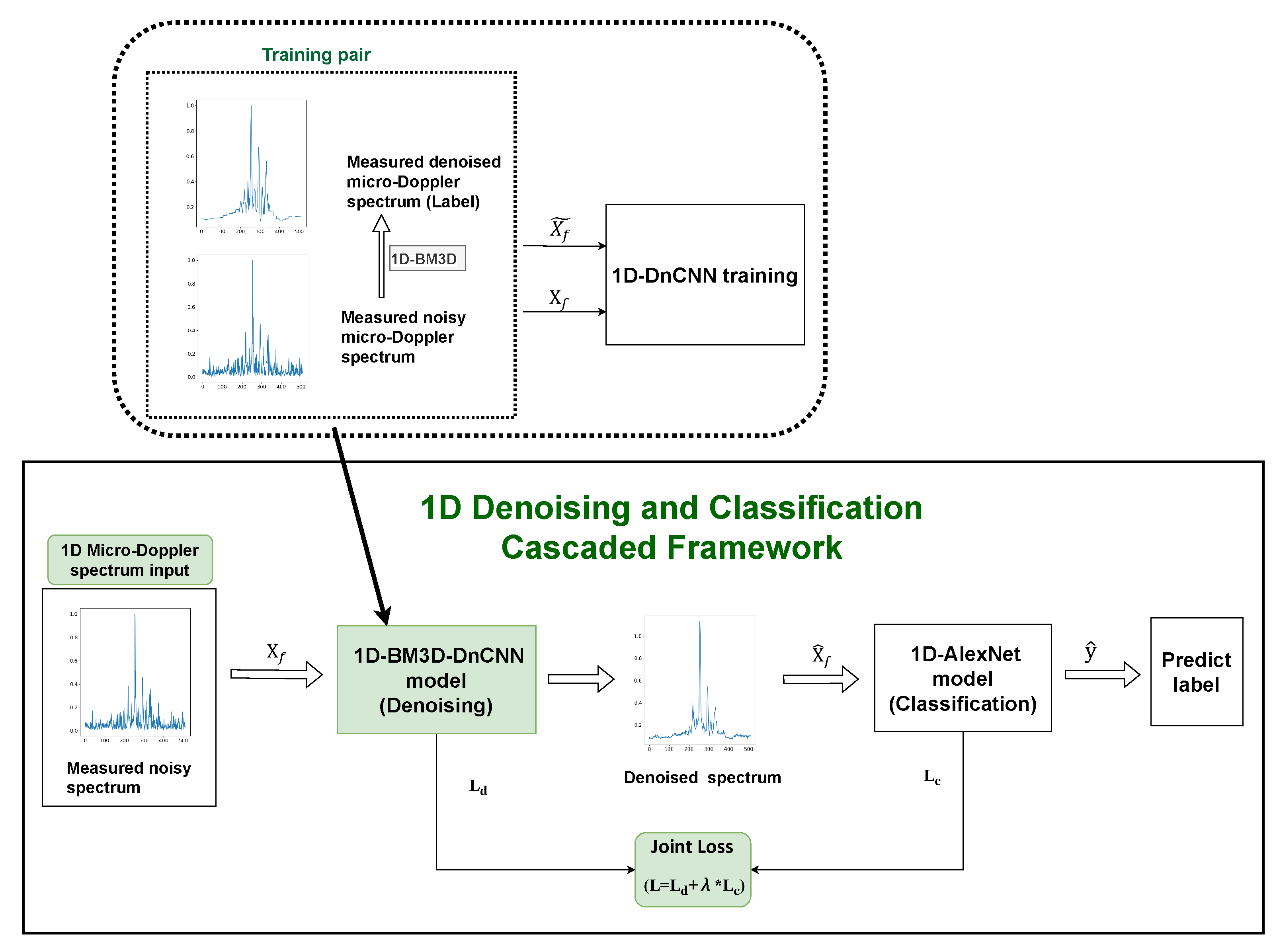
In this paper, a 1D denoising and classification cascaded framework based on the micro-Doppler spectrum is proposed to effectively classify low-resolution radar targets. The proposed framework is efficiently designed with two cascaded sub-networks to achieve classification decisions within one CPI period, which has the advantages of high real-time efficiency and low computational load, especially under the challenging conditions of a low resolution and short dwell time in traditional pulse radar systems. The first denoising subnetwork addresses radar micro-Doppler spectrum denoising, in which an improved 1D-DnCNN model is proposed to enhance the quality of micro-Doppler signatures that may be affected by noise or exhibit weak signals. The second classification subnetwork utilizes an AlexNet-based architecture for the classification task, where a joint loss is calculated to facilitate the simultaneous optimization of the denoising subnetwork and contribute to achieving excellent classification performance.
The main contributions of this paper are summarized as follows.
This work develops a 1D signal-based network using the micro-Doppler spectrum to achieve the classification task based on a conventional pulsed radar system, as opposed to a 2D image-based network relying on the micro-Doppler spectrogram commonly used in existing studies.
We propose an improved 1D-DnCNN model that utilizes the 1D-BM3D algorithm to obtain ground truth labels for measured data, effectively addressing the challenge of training pair construction and enhancing denoising performance for 1D micro-Doppler spectrum, thereby ensuring high-quality input for the subsequent classification task.
We propose a cascaded framework with joint loss optimization, where the denoising subnetwork enhances micro-Doppler signatures degraded by noise and is integrated with the 1D-AlexNet classification subnetwork. By employing a joint loss function, our approach enables the synchronized optimization of both denoising and classification tasks. This design ensures outstanding classification performance, even under the challenges of a low resolution and short dwell time in the surveillance radar system.
Validated on both simulated and measured radar data, the proposed 1D cascaded framework demonstrates outstanding multi-target classification performance compared to separately trained denoising and classification models. Furthermore, compared to 2D-based networks, it offers superior real-time efficiency and lower computational complexity.
The remainder of this paper is organized as follows:
Section 2 reviews related work in the field. The proposed framework is presented in detail in
Section 3.
Section 4 presents the experimental setup and implementation details. In
Section 5, we provide a comprehensive evaluation of the framework, including experimental results and performance analysis.
Section 6 discusses the limitations of our work and suggests future research directions. Finally,
Section 7 concludes this paper.
3. Methods
In this section, the proposed 1D denoising and classification cascaded framework is presented with a comprehensive description below. The overall architecture is visually depicted in
Figure 1.
As illustrated in
Figure 1, the entire framework consists of two cascaded subnetworks for denoising and classification. The raw radar signal first undergoes Fourier transform and clutter removal as preprocessing steps. The resulting 1D micro-Doppler spectra serve as the input for subsequent processing. With labels generated by applying the 1D-BM3D algorithm to the measured micro-Doppler spectra, the 1D-DnCNN denoising model is trained using measured training pairs, effectively enhancing the micro-Doppler signatures within the Doppler spectra. The whole process is implemented using a cascaded approach, where the denoising and classification models are connected with a joint loss function. This collaborative training strategy facilitates synchronized optimization of the denoising and classification models, creating a unified framework that can classify radar targets accurately.
3.1. 1D Micro-Doppler Spectrum Input
In a pulse-Doppler radar system, a sequence of N coherent pulses is transmitted with a specified Pulse Repetition Interval (PRI). The received echo is processed through quadrature demodulation, resulting in two-channel signals: In-phase (I) and Quadrature phase (Q). One CPI is commonly employed as the processing unit for target detection and tracking in a pulsed-Doppler radar system, serving as a standard design choice. For a detected moving target, the received one-CPI baseband signal can be expressed as
where
N is the number of accumulated pulses;
is the pulse index;
and
are I and Q samples of the
n-th received pulse, respectively.
The spectrum
can be obtained from the Discrete Fourier Transform of
, primarily reflecting the Doppler speed of the moving target.
where
is the frequency index.
The spectrogram
captures time-varying frequency modulation information based on Short-Time Fourier Transform (STFT) [
3], which is calculated by windowing the signal
with a sliding window and then computing the Discrete Fourier Transform of the windowed signal.
where
is the window function of length
L,
;
represents the step size; the entire signal
of length
N is divided into
T segments,
;
is the frequency index, and
is the time index. STFT is a widely used time–frequency domain method for micro-Doppler analysis in radar signals. Mainstream radar target classification methods leverage time–frequency domain information, typically using the spectrogram
as the 2D input image.
In this paper, we propose utilizing the spectrum
as a 1D input vector in the frequency domain, in contrast to the spectrogram
in the time–frequency domain. We examine the micro-Doppler differences in spectrogram and spectrum for various radar targets, using human walking and running as a comparative example.
Figure 2 illustrates the micro-Doppler distributions of radar returns for walking and running individuals, presenting both the spectrogram
for a prolonged observation time and the Doppler spectrum
for a one-CPI time. The left images in
Figure 2a,b depict spectrograms derived from 30 frames of radar returns for human running and walking. These two images last approximately 2.5 s, revealing a stable and periodic micro-Doppler phenomenon with sinusoidal-like changes in velocity during a gait. It is evident that walking and running motions exhibit distinct micro-Doppler signatures owing to their different gait patterns. Walking typically manifests a slower pattern and weaker micro-Doppler component, in contrast to the faster pattern and stronger micro-Doppler component associated with running.
However, obtaining more pronounced micro-Doppler differences with a long observation time, as shown in the left pictures, may not be practical for the pulsed radar system used in this study. It is impossible to achieve continuous accumulation for a moving target due to discontinuous observation and a short dwell time, especially in the Track-And-Scan (TAS) mode. Therefore, achieving one-CPI recognition becomes more meaningful in engineering applications. Moreover, despite the limitations in observation time, the Doppler spectrum can provide valuable information about the main Doppler shift and micro-Doppler sidebands. It effectively highlights unique micro-Doppler signatures associated with different micro-motions, while also having the capability to distinguish various radar targets.
Clutters present in radar returns often result in unwanted peaks at the zero-Doppler frequency. We employ the CLEAN technique [
44] to effectively remove the clutter. As illustrated in
Figure 3, the Clean algorithm effectively removes clutter from the raw Doppler spectrum while preserving the integrity of micro-Doppler components, ensuring no distortion during the process. The resultant spectrum after clutter removal, is referred to as the micro-Doppler spectrum, serving as the input for the proposed framework.
3.2. 1D-BM3D-DnCNN Model for Denoising
In this subsection, we present an improved 1D-DnCNN model, combined with the 1D-BM3D algorithm (referred to as 1D-BM3D-DnCNN), as an effective solution for denoising the 1D micro-Doppler spectrum.
3.2.1. 1D-DnCNN Denoising Subnetwork
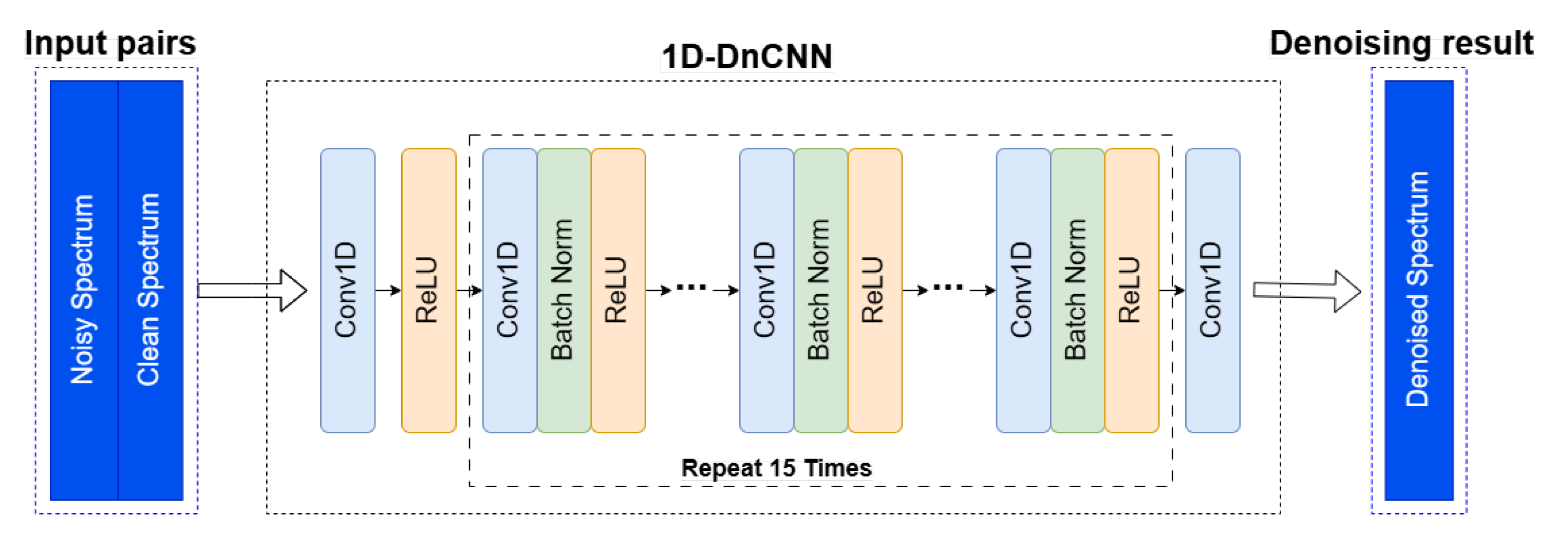
The utilization of residual learning in DnCNN allows the network to efficiently estimate noise from the noisy input. Additionally, the integration of batch normalization further enhances the training speed and contributes to the overall denoising efficacy. The DnCNN model adopts a 1D structure, as illustrated in
Figure 4.
The denoising model training involves inputting pairs of noisy and clean spectra, both represented as 1D series rather than 2D images. The convolution operations in the DnCNN model are adjusted for 1D input. The shape of the input samples for both noisy and clean spectra is
, where
B represents the batch size, and
H is the length of the radar spectrum. It is stated in [
25] that increasing the depth expands the receptive field of the network, enabling it to utilize contextual information from a larger image region. To balance performance and computational efficiency, a minimal depth of 17 was set, demonstrating that DnCNN can effectively compete with leading denoising methods. We consider it valuable to verify whether 1D-DnCNN with a similarly reduced depth, compared to 2D-CNN, can still achieve good denoising performance. Therefore, we applied 1D convolution to keep the dimension identical between the 1D input and output data of
and set the depth of the Conv+BN+ReLu module to 15 in our work, as shown in
Figure 4 for details.
Once fully trained, the denoising network, denoted as F, establishes a mapping between noisy and clean data. The denoising result is expressed as , where represents the denoised spectrum. The output of the denoising subnetwork, maintaining the size of , is then fed into the subsequent classification subnetwork, which is outlined in the following steps.
3.2.2. 1D-BM3D Algorithm
For the simulated dataset, training pairs can be easily generated using simulated data. However, obtaining clean data to serve as ground truth for the measured dataset is challenging. Some studies utilize simulated samples as labels for the measured samples. In our work, we propose applying the 1D-BM3D algorithm to pre-denoise the measured data, using the denoised samples as labels for the measured dataset.
BM3D is widely recognized as one of the most effective denoising algorithms for images. In this work, we adapt the algorithm for one-dimensional radar signals. The description of 1D-BM3D Algorithm Steps is illustrated in
Figure 5.
The modified process begins with block division, where the radar signal is segmented into overlapping blocks of fixed length to ensure sufficient redundancy for effective noise suppression. The 1D micro-Doppler spectrum
is divided into multiple overlapping 1D signal blocks. Given that the 1D spectrum
has a length of
, we set the length of each signal block to
with a stride of 1. The total number of signal blocks is then calculated as
. The
i-th block can be represented as
where
is the starting position of the
i-th block.
In the block matching step, similar blocks are identified within a predefined search window. For each reference block
, the similarity is evaluated using the Euclidean distance between blocks. The set of matched similar blocks is
where
is the distance between blocks
and
, and
is the similarity threshold. The reference block
and its matched blocks
are stacked into a two-dimensional array
:
where
are the similar blocks in
.
During collaborative filtering, the grouped blocks are transformed into a sparsity-promoting domain with the Discrete Cosine Transform (DCT), and noise reduction is performed using a thresholding operation. The two-dimensional array
undergoes DCT to obtain its transform domain representation:
where
is the transform operation. The transformed two-dimensional array
is represented as
where
is the transformed reference block, and
are the transformed similar blocks. In the transform domain, a hard thresholding operation is applied to
to remove noise components. The filtered result is
where
is the hard thresholding filter. The filtering formula is given by
where
is the threshold parameter.
Finally, in the aggregation step, the denoised blocks are combined to reconstruct the signal. The inverse transform is applied to the filtered two-dimensional array to obtain the denoised signal blocks:
The denoised signal blocks
are then aggregated to reconstruct the original one-dimensional signal. Since the blocks are overlapping, the final signal is obtained by weighted averaging:
where
is the weight function. The label
is generated by applying the 1D-BM3D algorithm to denoise the measured noisy spectrum
, thereby forming the training pair.
3.3. Cascaded Strategy with the Joint Loss Function
3.3.1. Cascaded Training Strategy
In our case, the ultimate objective is to accomplish the classification task based on the low-resolution radar. The denoising process proposed in
Section 3.2 is implemented to diminish the impact of noise, aiming for improved classification performance. As demonstrated in previous studies [
40,
42], an increase in SNR correlates with higher recognition accuracy. To perform classification, a classification model is cascaded following the denoising stage. We utilize the AlexNet as the foundational structure for the 1D classification subnetwork, as described in
Figure 6. To accommodate the 1D input, similar adjustments with the denoising subnetwork are made to the convolution and pooling operations. The modified structure ensures compatibility with the characteristics of 1D input data, allowing for an effective integration of the denoised spectrum into the classification model.
The joint training strategy of our proposed cascaded framework is illustrated in detail in
Figure 7. This framework integrates the denoising subnetwork (1D-BM3D-DnCNN) and the classification subnetwork (1D-AlexNet) into a unified model for joint training. The input data consist of three components: the 1D measured noisy spectrum
, the denoising label
, and the classification label
y. The pair
constitutes the training set for the denoising subnetwork, where the denoised output
serves as the input to the classification. Consequently, the pair
forms the the training set for the classification subnetwork. The entire cascaded model is optimized through a joint loss function
L, where
measures the loss of the denoising subnetwork between the denoised output and clean reference
, while
computes the loss of the classification subnetwork between the predicted class label and the ground truth label
.
3.3.2. Joint Loss Function
Our proposed cascaded framework is designed to enhance overall performance by leveraging the denoising process to better represent the input radar signals, thereby optimizing the effectiveness of the classification subnetwork. There are two loss components adopted in our proposed cascaded framework.
The reconstruction loss of the denoising subnetwork is the mean squared error (MSE) between the clean spectrum and the denoised spectrum, which can be represented as
where
is the ground truth spectrum;
is the denoised spectrum, obtained from the output of the denoising subnetwork
F, with the measured noisy spectrum
as the input;
indicates the
i-th element of
;
and
are of size
.
The loss of the classification subnetwork is the cross-entropy loss between the predicted label and the truth label. For a multi-classification problem, each class is labeled with an index corresponding to the radar target it represents, and the index is represented as an one-hot vector
y with M dimensions (as there are M classes in total). For instance, the first class can be represented as
. Let the the denoised spectrum
feed into the classification subnetwork, which is denoted as
. The output predicted label is then a M-dimensional vector
, where
. The cross-entropy loss between
y and
can be calculated as
where
y is the ground truth label,
represents the probability of the classified target belonging to the
i-th class, and
.
The joint loss is defined as the weighted sum of the reconstruction loss and the classification loss, which can be represented as
where
is the weight for balancing the losses
and
.
This joint optimization strategy creates a synergistic relationship between the denoising and classification tasks. The denoising subnetwork is trained to generate accurate outputs while preserving discriminative features essential for classification. Simultaneously, the classification subnetwork guides the denoiser to produce representations that enhance classification performance.
4. Experimental Setting
This section describes the experimental settings, including evaluation metrics, data collection, parameter settings, and the noise model.
4.1. Dataset Description
To evaluate the proposed method, six kinds of targets are considered: wheeled vehicle, tracked vehicle, person walking, person running, UAV, and ship. Wheeled and tracked vehicles are two typical targets for the vehicle classification task based on micro-Doppler signatures. In this case, a small van (Iveco Daily) and a tank are used as wheeled and tracked vehicle targets, respectively. The UAV target used for our experiments is a type of a quadcopter drone (DJI Phantom 4), and the ship target is a common medium-sized speedboat.
In our experiment, two datasets are used: a measured dataset and a simulated dataset.
4.1.1. Measured Dataset from X-Band Pulsed-Doppler Radar System
The real data collection from typical targets is performed based on a ground surveillance pulsed-Doppler radar. It is an X-band radar system with an emitted power of 15 W and the sampling frequency of 80 MHz. The coverage range is 0–360° in azimuth and 0–30° in elevation. The radar antenna has an azimuth beam width of 3° and an elevation beam width of 4.2°. This system has a low resolution of 15 m in distance due to a narrow bandwidth of 10 MHz. The number of coherent pulses
N is 256 and the PRI is 340 μs in one frame, and the lasting time for one CPI signal is calculated to be about 87 ms. The experimental scene with the radar system and target are shown in
Figure 8.
Classifying ground-moving and near-ground flying objects are important for applications such as perimeter security and surveillance. Due to the low resolution and short dwell time, the surveillance radar used in our experiment is often only required to achieve a rough classification of typical targets such as humans, vehicles, and UAVs. In our work, we expanded the typical targets to include six distinct classes in order to intensify the challenge of classification and test our proposed framework. A total of 6400 frames of six types of targets—wheeled vehicle (1300), tracked vehicle (1000), person walking (1100), person running (1000), UAV (1400), and ship (600)—are measured by the X-band surveillance radar system to perform relevant experiments. These data are collected from several kinds of scenes with the radar placed on the road or hillside to detect and track the targets. The detection range of targets covers a range from 100 m to 5 km.
4.1.2. Simulated Dataset for Denoising Model
We evaluate the denoising performance using the AWGN model in the experiment, a widely accepted assumption in denoising studies. This model is constructed using a zero-mean normal distribution based on the specified noise level (SNR).
4.2. Parameter Settings
In order to obtain training and test data, we selected the hierarchical sampling method for assessing the denoising performance and classification accuracy in our simulated and measured dataset in our experiments. Hierarchical sampling, also known as stratified sampling, is a method used to split a dataset into training and testing subsets, and each subset maintains the same proportion of each class as in the original dataset. This method can ensure that the class distribution in the training and testing datasets mirrors that of the original dataset, help in building more accurate and reliable models, especially for imbalanced datasets, and minimize the bias introduced by random sampling, where some classes might be underrepresented or overrepresented. In our work, we set the test size from 0.2 to 0.8, specifying that 20% to 80% of the data are used for testing sequentially. The parameter “stratify” was set to the label to ensure that the split was stratified based on the target variable label. The random state was set to 42 to ensure the reproducibility of the results. All models were trained for 200 epochs. The process needed to be repeated 5 times with randomly changed training samples to fairly evaluate the suggested strategy, and the calculated average value of these 5 repetitions was the final result.
All models in our work were trained and tested in the Keras framework of the Tensorflow backend. The GPU that we used was a NVIDIA Tesla P100 graphics card with a 16-GB memory.
5. Results
This section allows for a thorough assessment of the framework’s ability to denoise measured radar signals and accurately classify the radar targets.
5.1. Simulated Radar Spectrum Denoising Training
For the simulated data, AGWN was introduced into the simulated clean signal to assess the performance of the denoising subnetwork. The denoising subnetwork took the radar spectrums as input, and outputs the denoised spectrums. We created a training set for the DnCNN model from the clean simulated spectrums and AWGN noisy spectrums of six classes. We evaluated the proposed denoising subnetwork under nine noise levels, where SNR = −20, −15, −10, −5, 0, 5, 10, 15, 20 dB. Note that we simulated noise in complex radar signals by generating Gaussian noise for both the real and imaginary components separately. The noisy complex signal was then created by adding these noise components to the original signal.
Taking the UAV target as an example, we generated a clean simulated spectrum and AWGN noisy spectrums under nine noise levels. In our previous work [
45], we simulated the UAV rotor echo model and analyzed the micro-Doppler distribution characteristics of the UAV target, pointing out that the main Doppler component of the fuselage and the micro-motion component were distributed on both sides of the fuselage in the frequency spectrum. An example of the original, noisy, and denoised Doppler spectra for the UAV target is presented in
Figure 9. The clean spectrum samples were formed by randomly changing the moving speed of the fuselage and the strength of the rotors, as shown in
Figure 9a. The noisy spectra were created by adding clean simulated spectra with noise, and the examples with different noise levels are shown in
Figure 9b.
Figure 9c shows the spectra after being processed by the 1D-DnCNN denoising model proposed in this paper. It can be seen that the noise of different degrees is suppressed to a certain extent, but the denoising effect is related to the SNR of the previous noise addition. The higher the SNR, the better the restoration after denoising.
The clean spectrum samples were formed by randomly changing the moving speed of the fuselage and the strength of the rotors, as shown in
Figure 9a. The noisy spectra were created by adding clean simulated spectra with noise, and the examples with different noise levels are shown in
Figure 9b.
Figure 9c shows the spectra after being processed by the 1D-DnCNN denoising model proposed in this paper. It can be seen that the noise of different degrees is suppressed to a certain extent, but the denoising effect is related to the SNR of the previous noise addition. The higher the SNR, the better the restoration after denoising.
Here, the Root Mean Squared Error (RMSE) serves as a metric to quantify the difference between the denoised spectrum and the clean spectrum, which can be expressed as
Additionally, the SNR provides a direct measure of how the spectrum is affected by the introduced noise component:
where
is the ground clean spectrum, and
is the denoised spectrum. These two performance indicators help evaluate the effectiveness of the denoising subnetwork in mitigating the impact of noise on the signal.
Table 1 presents the improvements in SNR and RMSE values for both the noisy and denoised datasets. The results show a significant enhancement after applying the denoising model, while
Figure 10 shows the comparison curves of the two evaluation indicators before and after denoising, which also proves the effectiveness of the 1D-DnCNN denoising model. When adding the same noise level, both SNR and RMSE are significantly improved after denoising processing. As the noise level increases, the SNR and RMSE values improve, but the room for improvement is reduced.
5.2. Measured Radar Spectrum Denoising Training
For the simulated dataset, we can create a training pair by using the simulated clean data and artificially added noise. However, capturing clean data to serve as ground truth for the measured dataset is quite challenging. In our work, we attempt two training approaches to address this issue:
The first approach utilizes the simulated samples as labels for the measured samples.
The second approach applies the 1D-BM3D algorithm to pre-denoise the measured data, treating the denoised samples as labels for the measured samples.
Figure 11 presents the 1D-DnCNN denoiser trained using these two approaches. The details of the two approaches and a comparison of their denoising performance will be illustrated in the subsequent section.
For the first approach, the simulated data are constructed to reflect the micro-Doppler characteristics specific to the six target classes, aiming for correlation and consistency with the measured target data. This allows us to use the simulated data for 1D-DnCNN model training and ensure its effectiveness on the measured data.
The performance of the 1D-DnCNN denoising model is evaluated based on the classification accuracy achieved on the denoised data using the 1D-AlexNet model. For comparison, we also train Autoencoder (AE) and U-Net models and assess their denoising effectiveness. Specifically, the denoised outputs from the 1D-DnCNN, 1D-AE, and 1D-Unet models are individually fed into the 1D-AlexNet for classification. The split rate, which represents the ratio between the training and the testing sets, is set as 0.2/0.8, 0.3/0.7, 0.4/0.6, 0.5/0.5, 0.6/0.4, 0.7/0.3, and 0.8/0.2, respectively.
Figure 12 shows the classification performance under varying split rates after applying the three denoising models, demonstrating that the 1D-DnCNN model outperforms the other two models on our measured radar dataset.
In the second approach, the 1D-BM3D algorithm is applied to denoise the 1D measured radar spectrum samples, and the pre-denoised samples from the 1D-BM3D process serve as labels to guide the training of the 1D-DnCNN denoising model.
Using these two training approaches, we train the 1D-DnCNN model. Subsequently, the trained model is applied to the measured samples under both approaches, generating the corresponding denoised outputs, as shown in
Figure 11.
An example of both denoising training approaches on the measured Doppler spectra of six classes is presented in
Figure 13.
Figure 13a displays the measured radar Doppler spectra for the six classes, while
Figure 13b,c show the denoised spectra obtained using the two respective training approaches. The visual denoising results clearly show that the second approach performs better, as it not only removes noise but also preserves the micro-Doppler signatures of various targets more effectively. A comparison of the classification performance of these two approaches will be provided in the next subsection.
5.3. Performance of the Proposed Cascaded Framework
Classification is the ultimate objective of our work, and we utilized an AlexNet-based deep network in our framework to perform this task. For the cascaded classification framework, we trained our model on the measured radar dataset obtained from an X-Band pulsed-Doppler radar system, as described in
Section 4.1.1. The joint loss in our framework is composed of the reconstruction loss from the denoising subnetwork and the classification loss from the 1D-AlexNet subnetwork, as defined in Equation (
4), where the weight parameter
is empirically set to 2. The split rate is set as 0.8/0.2.
The loss and accuracy curves for the training and testing datasets are shown in
Figure 14, demonstrating that our proposed method achieves excellent performance. The final classification accuracy exceeds 95%, with only a minimal gap between the training and testing accuracy curves.
We also investigated how signal denoising can enhance the classification task over the measured dataset from an X-Band pulsed-Doppler Radar system. The noisy radar spectrums of six target classes were denoised and then fed into the 1D-AlexNet network for the classification task. To evaluate how different denoising schemes contribute to the classification performance, we experimented with the following cases:
The measured radar spectrums were directly fed into the 1D-AlexNet classification network, termed as 1D-AlexNet. This scheme served as the baseline.
The measured radar spectrums were first denoised using the 1D-BM3D algorithm and then fed into the 1D-AlexNet classification network, termed as 1D-BM3D + AlexNet.
The measured radar spectrums were denoised using the separately trained 1D-DnCNN denoising network with the simulated dataset, and then fed into the 1D-AlexNet classification network, termed as 1D-DnCNN (Separate) + AlexNet.
The measured radar spectrums were denoised using the separately trained 1D-DnCNN denoising network with the measured dataset where the ground truth was generated by the 1D-BM3D algorithm, and then fed into the 1D-AlexNet classification network, termed as 1D-DnCNN with BM3D (Separate) + AlexNet.
Our proposed scheme: The measured radar spectrums were processed through the cascaded framework consisting of the 1D-DnCNN denoising subnetwork based on 1D-BM3D and the 1D-AlexNet classification subnetwork, which was trained using the joint loss, termed as Joint Training (Proposed).
Table 2 presents the classification performance for the five cases described above. Additionally, we investigated the effects of varying the split rate, including 0.2/0.8, 0.3/0.7, 0.4/0.6, 0.5/0.5, 0.6/0.4, 0.7/0.3, and 0.8/0.2.
Figure 15 shows that the accuracy trend as the training set proportion increases from 0.2 to 0.8. It is clear that accuracy improves as the training set proportion increases. It can be observed that the baseline 1D-AlexNet scheme yields significantly lower accuracy than the other four cases for all split rates, highlighting the importance of denoising as a preprocessing step for the classification task on measured radar data. When denoising preprocessing methods like 1D-BM3D + AlexNet or separate denoising training methods like 1D-DnCNN (Separate) + AlexNet were applied, the accuracy improved compared to the baseline. As shown in
Table 2 and
Figure 15, our proposed joint training approach achieved the highest accuracy among all cases, demonstrating the effectiveness of the cascaded denoising and classification framework.
6. Discussion
We propose a 1D-based model that demonstrates excellent classification performance when validated on both simulated and measured radar data, outperforming separately trained denoising and classification models. In contrast to most current studies that employ 2D time–frequency spectrograms as input to deep network models, our approach utilizes the 1D micro-Doppler spectrum as input, significantly reducing computational complexity while maintaining competitive accuracy.
Table 3 presents a comparison between 1D-based and 2D-based models in terms of parameters, training time, and testing time.
In
Table 3, the “1D-DnCNN-AlexNet” model represents our proposed framework, which cascades 1D-DnCNN and 1D-AlexNet and takes the 1D micro-Doppler spectrum as input. For comparison, we also evaluate the “2D-DnCNN-AlexNet” model, which cascades 2D-DnCNN and 2D-AlexNet and processes 2D time–frequency spectrograms as input. The results demonstrate that, compared to 2D-based networks, the 1D-DnCNN-AlexNet model achieves a reduction in the number of parameters while also exhibiting faster training and testing speeds, making it more efficient for real-time applications.
While this paper demonstrates promising results, several limitations should be noted. Our work conducts classification experiments exclusively using real measured data from a narrow-band pulse radar, and the generalization capability of the proposed model across other datasets has yet to be validated. Furthermore, due to the high cost of radar data acquisition, the number of real measured samples used in this study is relatively limited. The scarcity of labeled data also imposes constraints on the training performance of deep learning models. Future work will focus on evaluating the adaptability of the model to various radar systems and environmental conditions to enhance its robustness across a wider range of applications. Additionally, we aim to explore the fine classification of similar targets, such as various types of vehicles or UAVs, which presents a greater challenge given the constraints of low-resolution radar.


