Bayesian Distributed Target Detectors in Compound-Gaussian Clutter Against Subspace Interference with Limited Training Data

Abstract

In this article, the problem of Bayesian detecting rank-one distributed targets under subspace interference and compound Gaussian clutter with inverse Gaussian texture is investigated. Due to the clutter heterogeneity, the training data may be insufficient. To tackle this problem, the clutter speckle covariance matrix (CM) is assumed to obey the complex inverse Wishart distribution, and the Bayesian theory is utilized to obtain an effective estimation. Moreover, the target echo is assumed to be with a known steering vector and unknown amplitudes across range cells. The interference is regarded as a steering matrix that is linearly independent of the target steering vector. By utilizing the generalized likelihood ratio test (GLRT), a Bayesian interference-canceling detector that can work in the absence of training data is derived. Moreover, five interference-cancelling detectors based on the maximum a posteriori (MAP) estimate of the speckle CM are proposed with the two-step GLRT, the Rao, Wald, Gradient, and Durbin tests. Experiments with simulated and measured sea clutter data indicate that the Bayesian interference-canceling detectors show better performance than the competitor in scenarios with limited training data.

1. Introduction

The problem of detecting a distributed target in sea clutter has been widely studied in the maritime radar field during these years [1,2]. The generalized likelihood ratio test [3] (GLRT) was first utilized to construct the adaptive detectors. Other criteria like Rao and Wald tests have been investigated subsequently over time.

The design of an adaptive detector is closely tied to the clutter model. Therefore, an accurate and appropriate model can substantially improve detection performance. The clutter obtained by high-resolution radar usually shows spikiness, implying that the probability density function (PDF) of the clutter power shows heavy-tailed, which is different from the Rayleigh distribution [4]. To characterize the non-Rayleigh clutter, the compound-Gaussian (CG) model is commonly adopted. Under the CG model, the clutter can be decomposed into two quantities, named texture and speckle component. The former varies gradually over time and can be considered approximately constant within a coherent processing interval at each range cell [5].

The gamma texture was first investigated for describing the sea clutter [6]. However, in some scenarios, the gamma texture was found to be mismatched and resulted in performance loss. Therefore, other textures such as lognormal texture [7], generalized inverse Gaussian texture [8], and inverse Gaussian (IG) texture have been proposed. Moreover, in [1], the authors proved that the IG texture can fit the sea clutter better than the other texture distributions in most situations.

In contrast to the texture component, the speckle component is a random vector obeying zero-mean complex Gaussian distribution with an unknown covariance matrix (CM). The estimation of the speckle CM is of great significance in adaptive detection. An accurate estimation of the CM can be used to suppress the clutter efficiently, hence raising the probability of detection (PD) [9]. To estimate the CM, a secondary dataset, located around the testing data, is employed. However, in some scenarios, the training data may be insufficient. Thus, investigating the estimate of the speckle CM with limited training data is meaningful in improving the detection performance in practice.

Many approaches have been proposed to estimate the clutter CM. Traditional methods contain the sample covariance matrix (SCM) estimator [3], the normalized sample covariance matrix (NSCM) estimator [10], the constrained approximate maximum likelihood (constrained AML) estimator [11,12], and the CM estimator based on geometry barycenters [13]. When the environment is homogeneous or partially homogeneous, the structure of the CMs in cells under test (CUTs) and reference cells are the same, the above methods can estimate the CM accurately and result in acceptable performance of the detectors. However, in some situations, the homogeneous clutter environment model may not be suitable [12,14]. In this case, the structure of the clutter CM in each range cell may be different, resulting in insufficient training data and great performance degradation of the mentioned estimators. To overcome this, some efficient methods have been studied. Aboutanios derived a hybrid detection approach and proposed the use of the generalized inner product as a heterogeneity measure [15]. In [16], Aubry gave an approach for CM estimation based on the geometric diagram. Additionally, in [17], the authors regarded the CM as a random quantity obeying inverse complex Wishart distribution [18], and utilizing Bayesian theory to construct an adaptive detector for a point-like target with limited training data. Subsequently, Bandiera [19] proposed a range-distributed target detector based on the GLRT for CG clutter with gamma texture, and the experiments indicated that the detectors showed better performance than the other detectors. Xue [20] investigated knowledge-aided detection in IG texture CG clutter and assessed the detection performance via simulated and measured data experiments. Guo [21] considered the detection of rank-one distributed target embedded in lognormal texture CG clutter and proposed several Bayesian detectors that can work with limited training data or even no training data by incorporating the maximum a posteriori (MAP)-estimated speckle CM and texture component.

The detectors discussed are primarily designed for point-like or range-distributed targets in the absence of interference. However, in real-world detection scenarios, radar echoes are often contaminated by interference from sources such as civil broadcasting systems or electronic countermeasures, in addition to clutter and target signals [22,23]. The interference received by radar will lead to false alarm points and seriously degrade the detection performance [24]. By utilizing the electronic support measures [25], prior information on the interference can be obtained. In this case, the interference can be called subspace interference.

Considering the existence of subspace interference, motivated by the Bayesian approach, in this paper, we aim to detect the range-distributed targets under subspace interference in IG texture CG clutter. Additionally, the speckle CM is assumed to be random and obeys the complex inverse Wishart distribution. The innovations and contributions of this article are as follows:

(1)

We derive six Bayesian interference-canceling detectors under CG clutter with inverse Gaussian texture. The first GLRT-based detector can work in the absence of training data while the others combine prior information on the speckle CM and training data to obtain higher estimate precision of the CM to enhance the performance.

(2)

The Bayesian interference-canceling detectors for range-distributed targets embedded in CG clutter with IG texture and subspace interference are first proposed.

(3)

Simulated and IPIX radar-measured data are utilized to confirm the effectiveness of the proposed detectors and their superiority to the competitors in most situations.

The rest of the article is organized as follows. We give the problem formulation and declaration of signal, interference, and clutter models in Section 2. Then, we derive six Bayesian interference-canceling detectors in Section 3. The effectiveness of the proposed detectors is carried out in Section 4 throughout experiments. Finally, we conclude this article in Section 5.

Notations: Matrices/vectors are written in uppercase/lowercase bold letters. ${(\cdot )}^{*}$, ${(\cdot )}^T$ and ${(\cdot )}^H$ represents conjugate, transpose, and conjugate transpose, respectively. ${(\cdot )}^{-1}$, ${(\cdot )}^{1/2}$, and ${(\cdot )}^{-1/2}$ denotes the inverse, square root, and inverse square root of a square matrix. $\otimes$ denotes the Kronecker product. $\mathrm{tr}(\cdot )$ denotes the trace. $\ln (\cdot )$ represents the natural logarithm. $\det (\cdot )$ denotes the determinant. $\left|\cdot \right|$ is the absolute value of a scalar. ${‖\cdot ‖}_2$ denotes the 2-norm of a column vector. $\mathcal{C}{\mathcal{W}}^{-1}(\cdot )$ denotes the complex inverse Wishart distribution. $\mathrm{E}(\cdot )$ denotes the statistical expectation. $\propto$ and $~$ means “is proportional to” and “is distributed as”, $\mathsf{\Gamma }(\cdot )$ is the Euler’s gamma function. $diag(\cdot )$ is the diagonal matrix. $0_{a\times b}$ denotes the $a\times b$ dimensional zero matrix.

2. Problem Formula

There exists an $N\times K$ complex matrix $X$ representing the testing data collected by a radar system with $N$ pulses across $K$ range cells (also called CUT). The echo of the distributed target is with a known steering vector but unknown amplitudes, having the form $H=s{a}^H$, where the $N\times 1$ complex vector $s$ is the target steering vector, and $K\times 1$ complex vector $a$ denotes the complex amplitudes of the target in different range cells. The clutter component is represented by $C$. Each column of $C$ is modeled as CG clutter. Thus, we have

$$C=N{\Lambda }^{1/2}$$

(1)

where $\Lambda =diag({\dot{\mathbf{𝔯}}}_1,\dots ,{\dot{\mathbf{𝔯}}}_K)$ is a diagonal matrix with non-zero elements being the texture components corresponding to a specific range cell.

In this article, the texture component in range cells is regarded as obeying the IG distribution [26], i.e.,

$$f({\dot{\mathbf{𝔯}}}_k)=\sqrt{{\displaystyle \frac{{\lambda }_k}{2\pi }}}{\dot{\mathbf{𝔯}}}_k^{-3/2}\exp \left[-{\lambda }_k({\displaystyle \frac{{\dot{\mathbf{𝔯}}}_k}{2{\mu }_k^2}}+{\displaystyle \frac{1}{{\mu }_k}}+{\displaystyle \frac{1}{2{\dot{\mathbf{𝔯}}}_k}})\right]$$

(2)

where ${\lambda }_k$ and ${\mu }_k$ denote the shape and scale parameter in $k$-th range cell, respectively.

In addition, each column of $N$, named speckle component, is independent and identically Gaussian distributed with an $N\times N$ CM $R$ and zero mean. To estimate the speckle CM $R$, the clutter-only training data matrix $X_L$ with length $L$ is usually assumed available.

However, when the training data is insufficient, the estimate precision of $R$ may degrade seriously. To settle this problem, the CM $R$ is considered to obey the complex inverse Wishart distribution with degree of freedom (DoF) $\nu$ and a scaled matrix $\Omega$ ($\nu >N$), i.e., $R\sim \mathcal{C}{\mathcal{W}}^{-1}(\nu ,\nu \Omega )$. The PDF of $R$ is given by [19,27]:

$$f\left(R\right)={\displaystyle \frac{{\det }^{-\left(\nu +N\right)}(R){\det }^{\nu }(\nu \Omega )\exp \left[-\mathrm{tr}\left(\nu R^{-1}\Omega \right)\right]}{{\pi }^{(N^2-N)/2}{\displaystyle \prod _{i=1}^N\mathsf{\Gamma }\left(\nu -i+1\right)}}}$$

(3)

where $\Omega$ and $\nu$ can be regarded as the prior information for the speckle CM $R$. In this article, $\Omega$ is estimated from the previously scanned data and $\nu$ is assumed known. Moreover, the DoF $\nu$ measures the distance between $R$ and $\Omega$. Specifically, $R$ is closer to $\Omega$ as $\nu$ gets larger.

Besides the target and clutter, we also consider the existence of subspace interference. Specifically, the interference can be represented by $Q=J\psi$, where $J$ is an $N\times q$ complex matrix which can be taken as the interference steering matrix, $\psi$ is an $q\times K$ complex matrix representing the coordinates of the interference.

Through the above discussion, the detection problem of rank-one distributed targets with subspace interference can be represented by the binary hypotheses test as follows:

$$\left\{\begin{array}{l}{H}_0:X=J\psi +C,X_L=C_L\\ H_1:X=s{a}^H+J\psi +C,X_L=C_L\end{array}\right.$$

(4)

For the above detection problem, the conditional PDFs of $X$ under two hypotheses are found to be:

$$f_0(\left.X\right|\Lambda ,R)={\displaystyle \frac{{\det }^{-K}(R)}{{\pi }^{NK}{\det }^N(\Lambda )}}\exp \left[-\mathrm{tr}\left(X_0^H{R}^{-1}{X}_0{\Lambda }^{-1}\right)\right]={\displaystyle \prod _{k=1}^K\frac{{\det }^{-1}(R)}{{\pi }^N{\dot{\mathbf{𝔯}}}_k^N}\exp \left(-\frac{x_{0,k}^H{R}^{-1}{x}_{0,k}}{{\dot{\mathbf{𝔯}}}_k}\right)}$$

(5)

$$f_1(\left.X\right|\Lambda ,R,a)={\displaystyle \frac{{\det }^{-K}(R)}{{\pi }^{NK}{\det }^N(\Lambda )}}\exp \left[-\mathrm{tr}\left(X_1^H{R}^{-1}{X}_1{\Lambda }^{-1}\right)\right]={\displaystyle \prod _{k=1}^K\frac{{\det }^{-1}(R)}{{\pi }^N{\dot{\mathbf{𝔯}}}_k^N}\exp \left(-\frac{x_{1,k}^H{R}^{-1}{x}_{1,k}}{{\dot{\mathbf{𝔯}}}_k}\right)}$$

(6)

where $X_1=X-s{a}^H-J\psi$, $X_0=X-J\psi$, $x_{1,k}=x_k-a_k^{*}s-J{\phi }_k$ is the $k$-th column of $X_1$, $x_{0,k}=x_k-J{\phi }_k$ is the $k$-th column of $X_0$, $a_k^{*}$ is the $k$-th element of $a^H$, ${\phi }_k$ is the $k$-th column of $\psi$, and ${\dot{\mathbf{𝔯}}}_k$ represents the texture component in $k$-th range cell.

3. Bayesian Interference-Canceling Detectors Design

In this section, we first propose a GLRT-based Bayesian interference-canceling detector that can work without training data. After that, we combine the training data, the DoF $\nu$ and the scaled matrix $\Omega$ to construct the interference-canceling detectors by the two-step GLRT, the Rao, Wald, Gradient, and Durbin tests, respectively.

3.1. BICGLRT-DT Detector

Combining the prior information of $R$ and $\dot{\mathbf{𝔯}}$, we can write the GLRT [3,21] for the detection problem in (4) as:

$${\displaystyle \frac{{\displaystyle \prod _{k=1}^K{\max }_{a_k,{\phi }_k,{\dot{\mathbf{𝔯}}}_k}f({\dot{\mathbf{𝔯}}}_k){\displaystyle \int f_1(\left.x_{1,k}\right|{\dot{\mathbf{𝔯}}}_k,R,a_k)f(R)\mathrm{d}R}}}{{\displaystyle \prod _{k=1}^K{\max }_{{\phi }_k,{\dot{\mathbf{𝔯}}}_k}f({\dot{\mathbf{𝔯}}}_k){\displaystyle \int f_0(\left.x_{0,k}\right|{\dot{\mathbf{𝔯}}}_k,R)f(R)\mathrm{d}R}}}}\underset{H_0}{\overset{H_1}{\gtrless }}{\eta }_{\mathrm{GLRT}}$$

(7)

where ${\eta }_{\mathrm{GLRT}}$ stands for the detecting threshold judged by a pre-assigned probability of false alarm (PFA). After some algebra and maximization, the maximized numerator and denominator of (7) is given as:

$$f({\dot{\mathbf{𝔯}}}_k){\displaystyle \int f_1(\left.x_{1,k}\right|{\dot{\mathbf{𝔯}}}_k,R,{\widehat{\phi }}_{1,k},{\widehat{a}}_k)f(R)\mathrm{d}R}\propto cf({\dot{\mathbf{𝔯}}}_k){\det }^{-1}(\Omega ){\dot{\mathbf{𝔯}}}_k^{-N}{\left(1+{\displaystyle \frac{Z_{1,k}}{{\dot{\mathbf{𝔯}}}_k}}\right)}^{-(\nu +1)}$$

(8)

where the detailed derivation can be seen in Appendix A, $P_{P_{\overline{J}}^{\perp }\overline{s}}^{\perp }=I_N-{P_{\overline{J}}^{\perp }\overline{s}{\overline{s}}^H{P}_{\overline{J}}^{\perp }/‖P_{\overline{J}}^{\perp }\overline{s}‖}_2^2$, and $Z_{1,k}={\overline{x}}_k^H{P}_{\overline{J}}^{\perp }{\overline{x}}_k/\nu -{({\overline{s}}^H{P}_{\overline{J}}^{\perp }\overline{s})}^{-1}|{\overline{x}}_k^H{P}_{\overline{J}}^{\perp }\overline{s}{|}^2/\nu$.

To estimate ${\dot{\tau }}_k$, we denote the following function:

$$Q({\dot{\mathbf{𝔯}}}_k)=f({\dot{\mathbf{𝔯}}}_k){\dot{\mathbf{𝔯}}}_k^{-N}{\left(1+{\displaystyle \frac{Z_{1,k}}{{\dot{\mathbf{𝔯}}}_k}}\right)}^{-(\nu +1)}\propto {\dot{\mathbf{𝔯}}}_k^{-N-3/2}{\left(1+{\displaystyle \frac{Z_{1,k}}{{\dot{\mathbf{𝔯}}}_k}}\right)}^{-(\nu +1)}\exp \left[-{\lambda }_k({\displaystyle \frac{{\dot{\mathbf{𝔯}}}_k}{2{\mu }_k^2}}+{\displaystyle \frac{1}{{\mu }_k}}+{\displaystyle \frac{1}{2{\dot{\mathbf{𝔯}}}_k}})\right]$$

(9)

Then, calculating the partial derivative of $\ln Q({\dot{\mathbf{𝔯}}}_k)$ with respect to (w.r.t.) ${\dot{\mathbf{𝔯}}}_k$ and nulling the result, we get:

$${\displaystyle \frac{\partial \ln Q({\dot{\mathbf{𝔯}}}_k)}{\partial {\dot{\mathbf{𝔯}}}_k}}=-(N+{\displaystyle \frac{3}{2}}){\displaystyle \frac{1}{{\dot{\mathbf{𝔯}}}_k}}+(\nu +1){\displaystyle \frac{Z_{1,k}}{{\dot{\mathbf{𝔯}}}_k^2+Z_{1,k}{\dot{\mathbf{𝔯}}}_k}}-{\lambda }_k({\displaystyle \frac{1}{2{\mu }_k^2}}-{\displaystyle \frac{1}{2{\dot{\mathbf{𝔯}}}_k^2}})=0$$

(10)

After some algebra, the equation for ${\dot{\mathbf{𝔯}}}_k$ under $H_1$ hypothesis can be written as:

$$\begin{array}{l}{\dot{\mathbf{𝔯}}}_k^3+{\overline{b}}_k{\dot{\mathbf{𝔯}}}_k^2-{\overline{c}}_k{\dot{\mathbf{𝔯}}}_k-{\overline{d}}_k=0\\ {\overline{b}}_k={\displaystyle \frac{{\mu }_k^2}{{\lambda }_k}}({\displaystyle \frac{{\lambda }_k}{{\mu }_k^2}}{Z}_{1,k}+2N+3)\\ {\overline{c}}_k={\displaystyle \frac{{\mu }_k^2}{{\lambda }_k}}(2\nu -2N-1)Z_{1,k}+{\mu }_k^2\\ {\overline{d}}_k={\mu }_k^2{Z}_{1,k}\end{array}$$

(11)

The roots of (11) can be given as [28]:

$$\begin{array}{l}{\dot{\mathbf{𝔯}}}_{km}=-{\displaystyle \frac{1}{3}}({\overline{b}}_k+y_m{\overline{T}}_k+{\displaystyle \frac{{\overline{\Delta }}_{k,0}}{y_m{\overline{T}}_k}})\\ m\in \{1,2,3\},y_1=1,y_2={\displaystyle \frac{-1+i\sqrt{3}}{2}},y_3={\displaystyle \frac{-1-i\sqrt{3}}{2}}\\ {\overline{T}}_k=\sqrt[3]{{\displaystyle \frac{{\overline{\Delta }}_{k,1}+\sqrt{{\overline{\Delta }}_{k,1}^2-4{\overline{\Delta }}_{k,0}^3}}{2}}}\\ {\overline{\Delta }}_{k,0}={\overline{b}}_k^2+3{\overline{c}}_k,{\overline{\Delta }}_{k,1}=2{\overline{b}}_k^3+9{\overline{b}}_k{\overline{c}}_k-27{\overline{d}}_k\end{array}$$

(12)

It has been proved in [28] that there is only one positive root for (11). Thus, we select the positive root ${\dot{\mathbf{𝔯}}}_{km},m\in \{1,2,3\}$ in (12) as the MAP estimate of ${\dot{\mathbf{𝔯}}}_k$ under $H_1$.

Substituting the MAP estimate ${\widehat{\dot{\mathbf{𝔯}}}}_{1,k}$ into (8) leads to

$$f({\widehat{\dot{\mathbf{𝔯}}}}_{1,k}){\displaystyle \int f_1(\left.x_{1,k}\right|{\widehat{\dot{\mathbf{𝔯}}}}_{1,k},R,{\widehat{\phi }}_{1,k},{\widehat{a}}_k)f(R)\mathrm{d}R}=cf({\dot{\mathbf{𝔯}}}_k){\det }^{-1}(\Omega ){\widehat{\dot{\mathbf{𝔯}}}}_{1,k}^{-N}{\left(1+{\displaystyle \frac{Z_{1,k}}{{\widehat{\dot{\mathbf{𝔯}}}}_{1,k}}}\right)}^{-(\nu +1)}$$

(13)

Similar to (13), the maximized PDF under $H_0$ hypothesis is written as:

$$f({\widehat{\dot{\mathbf{𝔯}}}}_{0,k}){\displaystyle \int f_1(\left.x_{0,k}\right|{\widehat{\dot{\mathbf{𝔯}}}}_{0,k},R,{\widehat{\phi }}_{0,k})f(R)\mathrm{d}R}=cf({\dot{\mathbf{𝔯}}}_k){\det }^{-1}(\Omega ){\widehat{\dot{\mathbf{𝔯}}}}_{0,k}^{-N}{\left(1+{\displaystyle \frac{Z_{0,k}}{{\widehat{\dot{\mathbf{𝔯}}}}_{0,k}}}\right)}^{-(\nu +1)}$$

(14)

where $Z_{0,k}={\overline{x}}_k^H{P}_{\overline{J}}^{\perp }{\overline{x}}_k/\nu$, and ${\widehat{\dot{\mathbf{𝔯}}}}_{0,k}$ is the positive root of the following equation:

$$\begin{array}{l}{\dot{\mathbf{𝔯}}}_k^3+{\overline{e}}_k{\dot{\mathbf{𝔯}}}_k^2-{\overline{f}}_k{\dot{\mathbf{𝔯}}}_k-{\overline{g}}_k=0\\ {\overline{e}}_k={\displaystyle \frac{{\mu }_k^2}{{\lambda }_k}}({\displaystyle \frac{{\lambda }_k}{{\mu }_k^2}}{Z}_{0,k}+2N+3)\\ {\overline{f}}_k={\displaystyle \frac{{\mu }_k^2}{{\lambda }_k}}(2\nu -2N-1)Z_{0,k}+{\mu }_k^2\\ {\overline{g}}_k={\mu }_k^2{Z}_{0,k}\end{array}$$

(15)

Finally, combining (13) and (14) with (7), after some algebra, we obtain the Bayesian interference-canceling GLRT detector for distributed target (BICGLRT-DT) as follows:

$${\displaystyle \sum _{k=1}^K\left[(N+\frac{3}{2})\ln \frac{{\widehat{\dot{\mathbf{𝔯}}}}_{0,k}}{{\widehat{\dot{\mathbf{𝔯}}}}_{1,k}}+(\nu +1)\ln \left(\frac{{\widehat{\dot{\mathbf{𝔯}}}}_{1,k}}{{\widehat{\dot{\mathbf{𝔯}}}}_{0,k}}\cdot \frac{{\widehat{\dot{\mathbf{𝔯}}}}_{0,k}+Z_{0,k}}{{\widehat{\dot{\mathbf{𝔯}}}}_{1,k}+Z_{1,k}}\right)+\frac{{\lambda }_k}{2{\mu }_k^2}({\widehat{\dot{\mathbf{𝔯}}}}_{0,k}-{\widehat{\dot{\mathbf{𝔯}}}}_{1,k})(1-\frac{{\mu }_k^2}{{\widehat{\dot{\mathbf{𝔯}}}}_{0,k}{\widehat{\dot{\mathbf{𝔯}}}}_{1,k}})\right]}\underset{H_0}{\overset{H_1}{\gtrless }}{\eta }_{BICGLRT-DT}$$

(16)

3.2. TD-BICGLRT-DT Detector

In this subsection, the DoF $\nu$, scaled matrix $\Omega$, and training data are adopted simultaneously to derive the interference-canceling detector based on two-step GLRT [29]. We first assume the $R$ and ${\dot{\mathbf{𝔯}}}_k$ are known, and the GLRT for (4) can be written as:

$${\displaystyle \frac{{\displaystyle \prod _{k=1}^K{\max }_{a_k,{\phi }_k}{f}_1(\left.x_{1,k}\right|{\dot{\mathbf{𝔯}}}_{1,k},a_k,{\phi }_k)f({\dot{\mathbf{𝔯}}}_{1,k})}}{{\displaystyle \prod _{k=1}^K{\max }_{{\phi }_k}{f}_0(\left.x_{0,k}\right|{\dot{\mathbf{𝔯}}}_{0,k},{\phi }_k)f({\dot{\mathbf{𝔯}}}_{0,k})}}}\underset{H_0}{\overset{H_1}{\gtrless }}{\eta }_{\mathrm{GLRT}}$$

(17)

where

$$f_1(\left.x_{1,k}\right|{\dot{\mathbf{𝔯}}}_{1,k},a_k,{\phi }_k)={\displaystyle \frac{{\det }^{-1}(R)}{{\pi }^N{\dot{\mathbf{𝔯}}}_{1,k}^N}}\exp \left[-{\displaystyle \frac{{(x_k-a_k^{*}s-J{\phi }_k)}^H{R}^{-1}(x_k-a_k^{*}s-J{\phi }_k)}{{\dot{\mathbf{𝔯}}}_{1,k}}}\right]$$

(18)

$$f_0(\left.x_k\right|{\dot{\mathbf{𝔯}}}_{0,k},{\phi }_k)={\displaystyle \frac{{\det }^{-1}(R)}{{\pi }^N{\dot{\mathbf{𝔯}}}_{0,k}^N}}\exp \left(-{\displaystyle \frac{{(x_k-J{\phi }_k)}^H{R}^{-1}(x_k-J{\phi }_k)}{{\dot{\mathbf{𝔯}}}_{0,k}}}\right)$$

(19)

Next, by calculating the partial derivative of (18) w.r.t. ${\phi }_k$ and nulling the result, we get the maximum likelihood estimate (MLE) of ${\phi }_k$ under $H_1$:

$${\widehat{\phi }}_{1,k}={\left(J^H{R}^{-1}J\right)}^{-1}{J}^H{R}^{-1}(x_k-a_k^{*}s)={\left(J_R^H{J}_R\right)}^{-1}{J}_R^H(x_{Rk}-a_k^{*}{s}_R)$$

(20)

where $J_R=R^{-1/2}J$, $x_{Rk}=R^{-1/2}{x}_k$ and $s_R=R^{-1/2}s$. Taking the derivative of (20) w.r.t. $a_k^{*}$, the MLE of $a_k$ is given as:

$${\widehat{a}}_k={x_{Rk}^H{P}_{J_R}^{\perp }{s}_R/‖P_{J_R}^{\perp }{s}_R‖}_2^2$$

(21)

where $P_{J_R}^{\perp }=I_N-J_R{\left(J_R^H{J}_R\right)}^{-1}{\stackrel{⌢}{J}}_R^H$.

Inserting (20) and (21) into (17), we yield:

$$f_1(\left.x_{1,k}\right|{\dot{\mathbf{𝔯}}}_{1,k},{\widehat{\phi }}_{1,k},{\widehat{a}}_k)={\displaystyle \frac{{\det }^{-1}(R)}{{\pi }^N{\dot{\mathbf{𝔯}}}_{1,k}^N}}\exp \left(-{\displaystyle \frac{{{\rm Y}}_{1,k}}{{\dot{\mathbf{𝔯}}}_{1,k}}}\right)$$

(22)

where ${{\rm Y}}_{1,k}=x_{Rk}^H{P}_{J_R}^{\perp }{x}_{Rk}-{(s_R^H{P}_{J_R}^{\perp }{s}_R)}^{-1}{\left|x_{Rk}^H{P}_{J_R}^{\perp }{s}_R\right|}^2={‖P_{P_{J_R}^{\perp }{s}_R}^{\perp }{P}_{J_R}^{\perp }{x}_{Rk}‖}_2^2$, and $P_{P_{J_R}^{\perp }{s}_R}^{\perp }=I_N-{P_{J_R}^{\perp }{s}_R{s}_R^H{P}_{J_R}^{\perp }/‖P_{J_R}^{\perp }{s}_R‖}_2^2$.

Similar to (22), we get

$$f_0(\left.x_{0,k}\right|{\dot{\mathbf{𝔯}}}_{0,k},{\widehat{\phi }}_{0,k})={\displaystyle \frac{{\det }^{-1}(R)}{{\pi }^N{\dot{\mathbf{𝔯}}}_{0,k}^N}}\exp \left(-{\displaystyle \frac{{{\rm Y}}_{0,k}}{{\dot{\mathbf{𝔯}}}_{0,k}}}\right)$$

(23)

where ${{\rm Y}}_{0,k}={‖P_{J_R}^{\perp }{x}_{Rk}‖}_2^2$.

Combining (22) and (23) with (17) leads to:

$${\displaystyle \frac{{\displaystyle \prod _{k=1}^K{\dot{\mathbf{𝔯}}}_{1,k}^{-N-3/2}\exp \left(-\frac{2{{\rm Y}}_{1,k}+{\lambda }_k}{2{\dot{\mathbf{𝔯}}}_{1,k}}-\frac{{\lambda }_k{\dot{\mathbf{𝔯}}}_{1,k}}{2{\mu }_k^2}\right)}}{{\displaystyle \prod _{k=1}^K{\dot{\mathbf{𝔯}}}_{0,k}^{-N-3/2}\exp \left(-\frac{2{{\rm Y}}_{0,k}+{\lambda }_k}{2{\dot{\mathbf{𝔯}}}_{0,k}}-\frac{{\lambda }_k{\dot{\mathbf{𝔯}}}_{0,k}}{2{\mu }_k^2}\right)}}}\underset{H_0}{\overset{H_1}{\gtrless }}{\eta }_{\mathrm{GLRT}}$$

(24)

Next, we estimate $R$ and ${\dot{\mathbf{𝔯}}}_k$. Taking the similar manner as (11), (12), and (15), the MAP of estimate of ${\dot{\mathbf{𝔯}}}_{1,k}$ and ${\dot{\mathbf{𝔯}}}_{0,k}$ is the positive root of the following two equations, respectively.

$$\begin{array}{l}{\dot{\mathbf{𝔯}}}_k^2+b_{Rk}{\dot{\mathbf{𝔯}}}_k-c_{Rk}=0\\ b_{Rk}={\displaystyle \frac{{\mu }_k^2}{{\lambda }_k}}(2N+3)\\ c_{Rk}=2{\displaystyle \frac{{\mu }_k^2}{{\lambda }_k}}{{\rm Y}}_{1,k}+{\mu }_k^2\end{array}$$

(25)

$$\begin{array}{l}{\dot{\mathbf{𝔯}}}_k^2+b_{Rk}{\dot{\mathbf{𝔯}}}_k-d_{Rk}=0\\ d_{Rk}=2{\displaystyle \frac{{\mu }_k^2}{{\lambda }_k}}{{\rm Y}}_{0,k}+{\mu }_k^2\end{array}$$

(26)

Combining (22), (23) and the estimated ${\widehat{\dot{\mathbf{𝔯}}}}_{1,k}$, ${\widehat{\dot{\mathbf{𝔯}}}}_{k,0}$ with (24), we obtain the detecting statistic:

$${\displaystyle \prod _{k=1}^K{\left(\frac{{\widehat{\dot{\mathbf{𝔯}}}}_{0,k}}{{\widehat{\dot{\mathbf{𝔯}}}}_{1,k}}\right)}^{N+3/2}\exp \left[\frac{{{\rm Y}}_{0,k}{\widehat{\dot{\mathbf{𝔯}}}}_{1,k}-{{\rm Y}}_{1,k}{\widehat{\dot{\mathbf{𝔯}}}}_{0,k}}{{\widehat{\dot{\mathbf{𝔯}}}}_{0,k}{\widehat{\dot{\mathbf{𝔯}}}}_{1,k}}+\frac{{\lambda }_k}{2{\mu }_k^2}({\widehat{\dot{\mathbf{𝔯}}}}_{0,k}-{\widehat{\dot{\mathbf{𝔯}}}}_{1,k})(1-\frac{{\mu }_k^2}{{\widehat{\dot{\mathbf{𝔯}}}}_{0,k}{\widehat{\dot{\mathbf{𝔯}}}}_{1,k}})\right]}\underset{H_0}{\overset{H_1}{\gtrless }}{\eta }_{BICGLRT-DT}$$

(27)

After that, to estimate $R$, the MAP approach is utilized. For the training data, the posterior PDF of $\Lambda$ and $R$ is:

$$\begin{array}{c}f(\left.\Lambda ,R\right|X_L)\propto f(R){\displaystyle \prod _{k=1}^{L}f({\dot{\mathbf{𝔯}}}_k)f_0(\left.x_{l,k}\right|{\dot{\mathbf{𝔯}}}_k,R)}\\ \hspace{1em}\hspace{1em}\hspace{1em}\hspace{1em}\hspace{1em}\hspace{1em}\hspace{1em}\hspace{1em}\propto {\det }^{-(\nu +L+N)}(R)\exp \left[-\mathrm{tr}\left(\nu R^{-1}\Omega \right)\right]\\ \hspace{1em}\hspace{1em}\hspace{1em}\hspace{1em}\hspace{1em}\hspace{1em}\hspace{1em}\hspace{1em}\hspace{1em}\hspace{1em}\hspace{1em}\hspace{1em}\times {\displaystyle \prod _{k=1}^L{\dot{\mathbf{𝔯}}}_k^{-(N+3/2)}\exp \left(-\frac{x_{l,k}^H{R}^{-1}{x}_{l,k}}{{\dot{\mathbf{𝔯}}}_k}-\frac{{\lambda }_k{\dot{\mathbf{𝔯}}}_k}{2{\mu }_k^2}-\frac{{\lambda }_k}{2{\dot{\mathbf{𝔯}}}_k}\right)}\end{array}$$

(28)

where $x_{l,k}$ is the column of $X_L$. After taking the partial derivative of (28) w.r.t. ${\dot{\mathbf{𝔯}}}_k$, we find that the MAP estimated ${\widehat{\dot{\mathbf{𝔯}}}}_{l,k}$ is the positive root of the equation as follows:

$$\begin{array}{l}{\widehat{\dot{\mathbf{𝔯}}}}_k^2+b_{Rk}{\widehat{\dot{\mathbf{𝔯}}}}_k-e_{Rk}=0\\ b_{Rk}={\displaystyle \frac{{\mu }_k^2}{{\lambda }_k}}(2N+3)\\ e_{Rk}=2{\displaystyle \frac{{\mu }_k^2}{{\lambda }_k}}{x}_{l,k}^H{R}^{-1}{x}_{l,k}+{\mu }_k^2\end{array}$$

(29)

Then, substituting ${\widehat{\dot{\mathbf{𝔯}}}}_{l,k}$ into (28), taking the logarithm of (28) and calculating the partial derivative of it w.r.t. $R$, the result is expressed as:

$$\begin{array}{c}{\displaystyle \frac{\partial \ln f(\left.R\right|\widehat{\Lambda },X_L)}{\partial R}}=-(\nu +L+N)R^{-T}+\nu R^{-T}{\Omega }^T{R}^{-T}-{\displaystyle \sum _{k=1}^L\frac{1}{{\widehat{\dot{\mathbf{𝔯}}}}_{l,k}}\frac{\partial x_{l,k}^H{R}^{-1}{x}_{l,k}}{\partial R}}\\ \hspace{1em}\hspace{1em}\hspace{1em}+{\displaystyle \sum _{k=1}^L\left(\frac{2x_{l,k}^H{R}^{-1}{x}_{l,k}+{\lambda }_k}{2{\widehat{\dot{\mathbf{𝔯}}}}_{l,k}^2}-\frac{N+3/2}{{\widehat{\dot{\mathbf{𝔯}}}}_{l,k}}-\frac{{\lambda }_k}{2{\mu }_k^2}\right)\frac{\partial {\widehat{\dot{\mathbf{𝔯}}}}_{l,k}}{\partial R}}\end{array}$$

(30)

Moreover, we yield

$${\displaystyle \frac{\partial x_{l,k}^H{R}^{-1}{x}_{l,k}}{\partial R}}=-R^{-T}{(x_{l,k}{x}_{l,k}^H)}^T{R}^{-T}$$

(31)

Combining (29) with (31), we obtain

$${\displaystyle \frac{\partial {\widehat{\dot{\mathbf{𝔯}}}}_{l,k}}{\partial R}}=-{\displaystyle \frac{2{\mu }_k^2{R}^{-T}{(x_{l,k}{x}_{l,k}^H)}^T{R}^{-T}}{2{\widehat{\dot{\mathbf{𝔯}}}}_{l,k}{\lambda }_k+{\mu }_k^2(2N+3)}}$$

(32)

Inserting (31) and (32) into (30), after some algebra, we yield the MAP estimate of $R$:

$${\widehat{R}}_{MAP}={\displaystyle \frac{\nu \Omega }{\nu +L+N}}+{\displaystyle \frac{1}{\nu +L+N}}{\displaystyle \sum _{k=1}^L\left[\frac{{\mu }_k^2\left(\frac{2x_{l,k}^H{R}^{-1}{x}_{l,k}+{\lambda }_k}{{\widehat{\dot{\mathbf{𝔯}}}}_{l,k}^2}-\frac{2N+3}{{\widehat{\dot{\mathbf{𝔯}}}}_{l,k}}-\frac{{\lambda }_k}{{\mu }_k^2}\right)}{2{\widehat{\dot{\mathbf{𝔯}}}}_{l,k}{\lambda }_k+{\mu }_k^2(2N+3)}+\frac{1}{{\widehat{\dot{\mathbf{𝔯}}}}_{l,k}}\right]x_{l,k}{x}_{l,k}^H}$$

(33)

It can be seen that ${\widehat{R}}_{MAP}$ is the function of itself and ${\widehat{\dot{\mathbf{𝔯}}}}_{l,k}$, and ${\widehat{\dot{\mathbf{𝔯}}}}_{l,k}$ is related to ${\widehat{R}}_{MAP}$. Therefore, ${\widehat{R}}_{MAP}$ needs to be solved by an iteration procedure. The initial matrix ${\widehat{R}}_{MAP}^{(0)}$ is constructed by the NSCM as follows:

$${\widehat{R}}_{NSCM}={\displaystyle \frac{N}{L}}{\displaystyle \sum _{k=1}^L\frac{x_{l,k}{x}_{l,k}^H}{x_{l,k}^H{x}_{l,k}}}$$

(34)

Moreover, to ensure $\mathrm{tr}({\widehat{R}}_{MAP}^{(i)})=N$ (where $i$ denotes the number of operated iterations) at the end of each iteration, the following process should be operated:

$${\widehat{R}}_{MAP}^{(i)}={\displaystyle \frac{N}{\mathrm{tr}({\widehat{R}}_{MAP}^{(i)})}}{\widehat{R}}_{MAP}^{(i)}$$

(35)

For the $i+1$-th iteration, the procedure can be listed as follows:

(1)

Calculating ${\widehat{\dot{\mathbf{𝔯}}}}_{l,k}^{(i)}$ by ${\widehat{R}}_{MAP}^{(i)}$ and (29).

(2)

Calculating ${\widehat{R}}_{MAP}^{(i+1)}$ based on ${\widehat{\dot{\mathbf{𝔯}}}}_{l,k}^{(i)}$ and (33).

(3)

Normalizing ${\widehat{R}}_{MAP}^{(i+1)}$ by (35).

After the iterations, we can obtain the ${\widehat{R}}_{MAP}$ as the MAP estimate of speckle CM $R$. Finally, inserting the estimated ${\widehat{R}}_{MAP}$ into (27), we obtain the statistic of training-data-based Bayesian interference-canceling GLRT detector for distributed target (TD-BICGLRT-DT):

$${\displaystyle \sum _{k=1}^K\left\{(N+\frac{3}{2})\ln \frac{{\widetilde{\dot{\mathbf{𝔯}}}}_{0,k}}{{\widetilde{\dot{\mathbf{𝔯}}}}_{1,k}}+\left[\frac{{\widetilde{{\rm Y}}}_{0,k}{\widetilde{\dot{\mathbf{𝔯}}}}_{1,k}-{\widetilde{{\rm Y}}}_{1,k}{\widetilde{\dot{\mathbf{𝔯}}}}_{0,k}}{{\widetilde{\dot{\mathbf{𝔯}}}}_{0,k}{\widetilde{\dot{\mathbf{𝔯}}}}_{1,k}}+\frac{{\lambda }_k}{2{\mu }_k^2}({\widetilde{\dot{\mathbf{𝔯}}}}_{0,k}-{\widetilde{\dot{\mathbf{𝔯}}}}_{1,k})(1-\frac{{\mu }_k^2}{{\widetilde{\dot{\mathbf{𝔯}}}}_{0,k}{\widetilde{\dot{\mathbf{𝔯}}}}_{1,k}})\right]\right\}}\underset{H_0}{\overset{H_1}{\gtrless }}{\eta }_{TD-BICGLRT-DT}$$

(36)

where ${\widetilde{{\rm Y}}}_{0,k}={‖P_{\tilde{J}}^{\perp }{\tilde{x}}_k‖}_2^2$, ${\widetilde{{\rm Y}}}_{1,k}={‖P_{P_{\tilde{J}}^{\perp }\tilde{s}}^{\perp }{P}_{\tilde{J}}^{\perp }{\tilde{x}}_k‖}_2^2$, ${\tilde{x}}_k={\widehat{R}}_{MAP}^{-1/2}{x}_k$, $\tilde{s}={\widehat{R}}_{MAP}^{-1/2}s$, $\tilde{J}={\widehat{R}}_{MAP}^{-1/2}J$, $P_{\tilde{J}}^{\perp }=I_N-\tilde{J}{({\tilde{J}}^H\tilde{J})}^{-1}{\tilde{J}}^H$, $P_{P_{\tilde{J}}^{\perp }\tilde{s}}^{\perp }=I_N-P_{\tilde{J}}^{\perp }\tilde{s}{\tilde{s}}^H{P}_{\tilde{J}}^{\perp }/{‖P_{\tilde{J}}^{\perp }\tilde{s}‖}_2^2$. ${\widetilde{\dot{\mathbf{𝔯}}}}_{1,k}$ and ${\widetilde{\dot{\mathbf{𝔯}}}}_{0,k}$ are the positive root of the following equations, respectively.

$$\begin{array}{l}{\dot{\mathbf{𝔯}}}_k^2+{\tilde{b}}_k{\dot{\mathbf{𝔯}}}_k-{\tilde{c}}_k=0\\ {\tilde{b}}_k={\displaystyle \frac{{\mu }_k^2}{{\lambda }_k}}(2N+3)\\ {\tilde{c}}_k=2{\displaystyle \frac{{\mu }_k^2}{{\lambda }_k}}{\widetilde{{\rm Y}}}_{1,k}+{\mu }_k^2\end{array}$$

(37)

$$\begin{array}{l}{\dot{\mathbf{𝔯}}}_k^2+{\tilde{b}}_k{\dot{\mathbf{𝔯}}}_k-{\tilde{d}}_k=0\\ {\tilde{d}}_k=2{\displaystyle \frac{{\mu }_k^2}{{\lambda }_k}}{\widetilde{{\rm Y}}}_{0,k}+{\mu }_k^2\end{array}$$

(38)

3.3. TD-BICRao-DT Detector

Assume $\Xi$ is the parameter set and has the form:

$$\Xi ={\left[{\Xi }_r^T,{\Xi }_s^T\right]}^T$$

(39)

where ${\Xi }_r=a^{*}$ and ${\Xi }_s={[({\dot{\mathbf{𝔯}}}_1,{\dot{\mathbf{𝔯}}}_2,\dots ,{\dot{\mathbf{𝔯}}}_K),{\phi }_1^T,{\phi }_2^T,\dots ,{\phi }_K^T]}^T={[t^T,f^T]}^T$, where $t={({\dot{\mathbf{𝔯}}}_1,{\dot{\mathbf{𝔯}}}_2,\dots ,{\dot{\mathbf{𝔯}}}_K)}^T$ and $f={[{\phi }_1^T,{\phi }_2^T,\dots ,{\phi }_K^T]}^T$. The Fisher information matrix (FIM) w.r.t. $\Xi$ is:

$$F\left(\Xi \right)=\mathrm{E}\left[{\displaystyle \frac{\partial \ln f_1(X_1)}{\partial {\Xi }^{*}}}{\displaystyle \frac{\partial \ln f_1(X_1)}{\partial {\Xi }^T}}\right]=-\mathrm{E}\left[{\displaystyle \frac{{\partial }^2\ln f_1(X_1)}{\partial {\Xi }^{*}\partial {\Xi }^T}}\right]$$

(40)

For convenience, partition the FIM as:

$$F\left(\Xi \right)=\left[\begin{array}{cc}{F}_{r,r}\left(\Xi \right)& F_{r,s}\left(\Xi \right)\\ F_{s,r}\left(\Xi \right)& F_{s,s}\left(\Xi \right)\end{array}\right]$$

(41)

The complex parameter Rao test [30] for (4) can be written as:

$${\left.{\displaystyle \frac{\partial \ln f_1(X_1)}{\partial {\Xi }_r}}\right|}_{\Xi ={\widehat{\Xi }}_0}^T{\left[F^{-1}({\widehat{\Xi }}_0)\right]}_{r,r}{\left.{\displaystyle \frac{\partial \ln f_1(X_1)}{\partial {\Xi }_r^{*}}}\right|}_{\Xi ={\widehat{\Xi }}_0}\underset{H_0}{\overset{H_1}{\gtrless }}{\eta }_{\mathrm{Rao}}$$

(42)

where ${\eta }_{Rao}$ denotes the detecting threshold, ${\widehat{\Xi }}_0$ is the MLE of $\Xi$ under $H_0$ hypothesis, and ${[F^{-1}({\widehat{\Xi }}_0)]}_{r,r}$ is the value of:

$${\left[F^{-1}(\Xi )\right]}_{r,r}={\left[F_{r,r}(\Xi )-F_{r,s}(\Xi )F_{s,s}^{-1}(\Xi )F_{s,r}(\Xi )\right]}^{-1}$$

(43)

at ${\Xi }_0$. Taking the partial derivative of logarithm of (6) w.r.t. $a^{*}$ and its conjugate leads to

$${\displaystyle \frac{\partial \ln f_1(X_1)}{\partial a^{*}}}={({\displaystyle \frac{1}{{\dot{\mathbf{𝔯}}}_1}}{s}^T{R}^{-T}{x}_{1,1}^{*},{\displaystyle \frac{1}{{\dot{\mathbf{𝔯}}}_2}}{s}^T{R}^{-T}{x}_{1,2}^{*},\dots ,{\displaystyle \frac{1}{{\dot{\mathbf{𝔯}}}_K}}{s}^T{R}^{-T}{x}_{1,K}^{*})}^T$$

(44)

$${\displaystyle \frac{\partial \ln f_1(X_1)}{\partial a}}={({\displaystyle \frac{1}{{\dot{\mathbf{𝔯}}}_1}}{s}^H{R}^{-1}{x}_{1,1},{\displaystyle \frac{1}{{\dot{\mathbf{𝔯}}}_2}}{s}^H{R}^{-1}{x}_{1,2},\dots ,{\displaystyle \frac{1}{{\dot{\mathbf{𝔯}}}_K}}{s}^H{R}^{-1}{x}_{1,K})}^T$$

(45)

Substituting (44) and (45) into (40) yields:

$$F_{r,r}\left(\Xi \right)=(s^H{R}^{-1}s){\Lambda }^{-1}={\Lambda }^{-1}\otimes (s^H{R}^{-1}s)$$

(46)

Calculating the partial derivative of (45) w.r.t. $t^T$ and taking the expectation, we obtain:

$$-\mathrm{E}\left[{\displaystyle \frac{{\partial }^2\ln f_1(X_1)}{\partial a\partial t^T}}\right]=-\mathrm{E}\left[\begin{array}{c}{s}^H{R}^{-1}{x}_{1,1}{\displaystyle \frac{\partial {\dot{\mathbf{𝔯}}}_1^{-1}}{\partial t^T}}\\ ⋮\\ s^H{R}^{-1}{x}_{1,K}{\displaystyle \frac{\partial {\dot{\mathbf{𝔯}}}_K^{-1}}{\partial t^T}}\end{array}\right]=0_{K\times K}$$

(47)

Similar to (47), taking the partial derivative of (45) w.r.t. $f^T$ and calculating the expectation, i.e.,

$$-\mathrm{E}\left[{\displaystyle \frac{{\partial }^2\ln f_1(X_1)}{\partial a\partial f^T}}\right]=-\mathrm{E}\left[\begin{array}{c}{\dot{\mathbf{𝔯}}}_1^{-1}{s}^H{R}^{-1}{\displaystyle \frac{\partial (x_1-a_1^{*}s-J{\phi }_1)}{\partial f^T}}\\ ⋮\\ {\dot{\mathbf{𝔯}}}_K^{-1}{s}^H{R}^{-1}{\displaystyle \frac{\partial (x_K-a_K^{*}s-J{\phi }_K)}{\partial f^T}}\end{array}\right]={\Lambda }^{-1}\otimes (s^H{R}^{-1}J)$$

(48)

Therefore, we have $F_{r,s}\left(\Xi \right)=[0_{K\times K},{\Lambda }^{-1}\otimes (s^H{R}^{-1}J)]$.

Next, to obtain the $F_{s,s}^{-1}(\Xi )$, we first take the partial derivative of (6) w.r.t. $t^{*}$ and $f^{*}$, respectively:

$${\displaystyle \frac{\partial \ln f_1(X_1)}{\partial t^{*}}}={(-{\displaystyle \frac{N}{{\dot{\mathbf{𝔯}}}_1}}+{\displaystyle \frac{x_{1,1}^H{R}^{-1}{x}_{1,1}}{{\dot{\mathbf{𝔯}}}_1^2}},-{\displaystyle \frac{N}{{\dot{\mathbf{𝔯}}}_2}}+{\displaystyle \frac{x_{1,2}^H{R}^{-1}{x}_{1,2}}{{\dot{\mathbf{𝔯}}}_2^2}},\dots ,-{\displaystyle \frac{N}{{\dot{\mathbf{𝔯}}}_K}}+{\displaystyle \frac{x_{1,K}^H{R}^{-1}{x}_{1,K}}{{\dot{\mathbf{𝔯}}}_K^2}})}^T$$

(49)

$${\displaystyle \frac{\partial \ln f_1(X_1)}{\partial f^{*}}}={({\displaystyle \frac{1}{{\dot{\mathbf{𝔯}}}_1}}{J}^H{R}^{-1}{x}_{1,1},{\displaystyle \frac{1}{{\dot{\mathbf{𝔯}}}_2}}{J}^H{R}^{-1}{x}_{1,2},\dots ,{\displaystyle \frac{1}{{\dot{\mathbf{𝔯}}}_K}}{J}^H{R}^{-1}{x}_{1,K})}^T$$

(50)

From (49) and (50) we can easily derive the following:

$$-\mathrm{E}\left[{\displaystyle \frac{\partial \ln f_1(X_1)}{\partial t^{*}\partial t^T}}\right]=-\mathrm{E}\left[\begin{array}{c}-N{\displaystyle \frac{\partial {\dot{\mathbf{𝔯}}}_1^{-1}}{\partial t^T}}+x_{1,1}^H{R}^{-1}{x}_{1,1}{\displaystyle \frac{\partial {\dot{\mathbf{𝔯}}}_1^{-2}}{\partial t^T}}\\ ⋮\\ -N{\displaystyle \frac{\partial {\dot{\mathbf{𝔯}}}_K^{-1}}{\partial t^T}}+x_{1,K}^H{R}^{-1}{x}_{1,K}{\displaystyle \frac{\partial {\dot{\mathbf{𝔯}}}_K^{-2}}{\partial t^T}}\end{array}\right]=N{\Lambda }^{-2}$$

(51)

$$-\mathrm{E}\left[{\displaystyle \frac{\partial \ln f_1(X_1)}{\partial t^{*}\partial f^T}}\right]=-\mathrm{E}\left[\begin{array}{c}{\displaystyle \frac{1}{{\dot{\mathbf{𝔯}}}_1^2}}{x}_{1,1}^H{R}^{-1}{\displaystyle \frac{\partial x_{1,1}}{\partial f^T}}\\ ⋮\\ {\displaystyle \frac{1}{{\dot{\mathbf{𝔯}}}_K^2}}{x}_{1,K}^H{R}^{-1}{\displaystyle \frac{\partial x_{1,K}}{\partial f^T}}\end{array}\right]=0_{K\times qK}$$

(52)

$$-\mathrm{E}\left[{\displaystyle \frac{\partial \ln f_1(X_1)}{\partial f^{*}\partial t^T}}\right]=-\mathrm{E}{\left[{\displaystyle \frac{\partial \ln f_1(X_1)}{\partial t^{*}\partial f^T}}\right]}^H=0_{qK\times K}$$

(53)

$$-\mathrm{E}\left[{\displaystyle \frac{\partial \ln f_1(X_1)}{\partial f^{*}\partial f^T}}\right]=-\mathrm{E}\left[\begin{array}{c}{\displaystyle \frac{1}{{\dot{\mathbf{𝔯}}}_1}}{J}^H{R}^{-1}{\displaystyle \frac{\partial x_{1,1}}{\partial f^T}}\\ ⋮\\ {\displaystyle \frac{1}{{\dot{\mathbf{𝔯}}}_K}}{J}^H{R}^{-1}{\displaystyle \frac{\partial x_{1,K}}{\partial f^T}}\end{array}\right]={\Lambda }^{-1}\otimes (J^H{R}^{-1}J)$$

(54)

Combining the above three equalities, we obtain:

$$F_{s,s}^{-1}(\Xi )=\left[\begin{array}{ll}{\displaystyle \frac{{\Lambda }^2}{N}}& 0_{K\times qK}\\ 0_{qK\times K}& \Lambda \otimes {(J^H{R}^{-1}J)}^{-1}\end{array}\right]$$

(55)

Inserting $F_{r,s}\left(\Xi \right)=[0_{K\times K},{\Lambda }^{-1}\otimes (s^H{R}^{-1}J)]$, (46) and (55) into (43) results in:

$$\begin{array}{l}{\left[F^{-1}\left({\Xi }_0\right)\right]}_{r,r}={[{\Lambda }^{-1}\otimes (s^H{R}^{-1}s)-{\Lambda }^{-1}\otimes s^H{R}^{-1}J{(J^H{R}^{-1}J)}^{-1}{J}^H{R}^{-1}s]}^{-1}\\ \hspace{1em}\hspace{1em}\hspace{1em}\hspace{1em}\hspace{1em}={[{\Lambda }^{-1}\otimes s_R^H{P}_{\stackrel{⌢}{J}}^{\perp }{s}_R]}^{-1}={\Lambda /‖P_{J_R}^{\perp }{s}_R‖}_2^2\end{array}$$

(56)

Besides, we notice that $a=0_{K\times 1}$ under $H_0$ hypothesis and ${\widehat{\phi }}_{0,k}={\left(J_R^H{J}_R\right)}^{-1}{J}_R^H{x}_{Rk}$. In the second step, inserting (44), (45), (56), the estimated ${\widetilde{\dot{\mathbf{𝔯}}}}_{0,k}$ in (38), and the estimated ${\widehat{R}}_{MAP}$ in (33) into (42), we obtain the statistic of training-data-based Bayesian interference-canceling Rao detector for distributed target (TD-BICRao-DT):

$${\displaystyle \sum _{k=1}^K\frac{{\tilde{x}}_k^H{P}_{\tilde{J}}^{\perp }\tilde{s}{\tilde{s}}^H{P}_{\tilde{J}}^{\perp }{\tilde{x}}_k}{{\widetilde{\dot{\mathbf{𝔯}}}}_{0,k}({\tilde{s}}^H{P}_{\tilde{J}}^{\perp }\tilde{s})}}={\displaystyle \sum _{k=1}^K\frac{{\tilde{x}}_k^H{P}_{P_{\tilde{J}}^{\perp }\tilde{s}}{\tilde{x}}_k}{{\widetilde{\dot{\mathbf{𝔯}}}}_{0,k}}}\underset{H_0}{\overset{H_1}{\gtrless }}{\eta }_{TD-BICRao-DT}$$

(57)

3.4. TD-BICWald-DT Detector

The complex parameter Wald test [30] for (4) is given by:

$${\left({\widehat{\Xi }}_{r,1}-{\Xi }_{r,0}\right)}^H{\left\{{\left[F^{-1}\left({\widehat{\Xi }}_1\right)\right]}_{r,r}\right\}}^{-1}\left({\widehat{\Xi }}_{r,1}-{\Xi }_{r,0}\right)\underset{H_0}{\overset{H_1}{\gtrless }}{\eta }_{\mathrm{Wald}}$$

(58)

where ${\eta }_{\mathrm{Wald}}$ is the detecting threshold, ${\widehat{\Xi }}_{r,1}$ is the MLE of ${\Xi }_r$ under $H_1$, and ${\widehat{\Xi }}_1$ is the MLE of $\Xi$ under $H_1$.

Inserting (56) and (21) into (58), ignoring the constant yields:

$$t_{\mathrm{Wald}}={\displaystyle \sum _{k=1}^K\frac{x_{Rk}^H{P}_{J_R}^{\perp }{s}_R{s}_R^H{P}_{J_R}^{\perp }{x}_{Rk}}{s_R^H{P}_{J_R}^{\perp }{s}_R{\dot{\mathbf{𝔯}}}_k}}={\displaystyle \sum _{k=1}^K\frac{x_{Rk}^H{P}_{P_{J_R}^{\perp }{s}_R}{x}_{Rk}}{{\dot{\mathbf{𝔯}}}_k}}$$

(59)

After that, inserting the estimated ${\widetilde{\dot{\mathbf{𝔯}}}}_{1,k}$ in (37) and the estimated ${\widehat{R}}_{MAP}$ in (33) into (59), we obtain the statistic of training-data-based Bayesian interference-canceling Wald detector for distributed target (TD-BICWald-DT):

$${\displaystyle \sum _{k=1}^K\frac{{\tilde{x}}_k^H{P}_{P_{\tilde{J}}^{\perp }\tilde{s}}{\tilde{x}}_k}{{\widetilde{\dot{\mathbf{𝔯}}}}_{1,k}}}\underset{H_0}{\overset{H_1}{\gtrless }}{\eta }_{TD-BICWald-DT}$$

(60)

3.5. TD-BICGradient-DT Detector

The complex value Gradient test [31] for (4) is given as follows:

$${\left.{\displaystyle \frac{\partial \ln f_1(X_1)}{\partial {\Xi }_r}}\right|}_{\Xi ={\widehat{\Xi }}_0}^T\left({\widehat{\Xi }}_{r,1}-{\Xi }_{r,0}\right)\underset{H_0}{\overset{H_1}{\gtrless }}{\eta }_{\mathrm{Gradient}}$$

(61)

where ${\eta }_{\mathrm{Gradient}}$ is the detecting threshold. Therefore, by inserting (21), (44), ${\widehat{\phi }}_{0,k}={\left({\stackrel{⌢}{J}}^H\stackrel{⌢}{J}\right)}^{-1}{\stackrel{⌢}{J}}^H{\stackrel{⌢}{x}}_k$, ${\widetilde{\dot{\mathbf{𝔯}}}}_{0,k}$ in (38) and the estimated ${\widehat{R}}_{MAP}$ into (61), we get the statistic of training-data-based Bayesian interference-canceling Gradient detector for distributed target (TD-BICGradient-DT):

$${\displaystyle \sum _{k=1}^K\frac{{\tilde{x}}_k^H{P}_{P_{\tilde{J}}^{\perp }\tilde{s}}{\tilde{x}}_k}{{\widetilde{\dot{\mathbf{𝔯}}}}_{0,k}}}\underset{H_0}{\overset{H_1}{\gtrless }}{\eta }_{TD-BICGradient-DT}$$

(62)

which is found to be the same as the TD-BICRao-DT in (57).

3.6. TD-BICDurbin-DT Detector

The complex value Durbin test [31] for (4) is denoted as:

$${\left({\widehat{\Xi }}_{r,01}-{\Xi }_{r,0}\right)}^H\left\{{\left[F\left({\widehat{\Xi }}_0\right)\right]}_{r,r}{\left[F^{-1}\left({\widehat{\Xi }}_0\right)\right]}_{r,r}{\left[F\left({\widehat{\Xi }}_0\right)\right]}_{r,r}\right\}\left({\widehat{\Xi }}_{r,01}-{\Xi }_{r,0}\right)\underset{H_0}{\overset{H_1}{\gtrless }}{\eta }_{\mathrm{Durbin}}$$

(63)

where ${\eta }_{\mathrm{Durbin}}$ is the detecting threshold, ${\widehat{\Xi }}_{r,01}$ is the MLE of ${\Xi }_r$ under $H_1$ with ${\Xi }_s={\widehat{\Xi }}_{s,0}$, ${\widehat{\Xi }}_{s,0}$ is the MLE of ${\Xi }_s$ under $H_0$. Consequently, we have

$${\widehat{\Xi }}_{s,0}={[({\widetilde{\dot{\mathbf{𝔯}}}}_{0,1},{\widetilde{\dot{\mathbf{𝔯}}}}_{0,2},\dots ,{\widetilde{\dot{\mathbf{𝔯}}}}_{0,K}),{\widehat{\phi }}_{0,1}^T,{\widehat{\phi }}_{0,2}^T,\dots ,{\widehat{\phi }}_{0,K}^T]}^T$$

(64)

And ${\widehat{\Xi }}_{r,01}$ is given by:

$${\widehat{\Xi }}_{r,01}=s_R^H{P}_{J_R}^{\perp }{x}_{Rk}/s_R^H{s}_R$$

(65)

Plugging (46), (56), (65), ${\widetilde{\dot{\mathbf{𝔯}}}}_{0,k}$ in (38) and the estimated ${\widehat{R}}_{MAP}$ into (63) results in the statistic of training-data-based Bayesian interference-canceling Durbin detector for distributed target (TD-BICDurbin-DT):

$${\displaystyle \sum _{k=1}^K\frac{{\tilde{x}}_k^H{P}_{P_{\tilde{J}}^{\perp }\tilde{s}}{\tilde{x}}_k}{{\widetilde{\dot{\mathbf{𝔯}}}}_{0,k}}}\underset{H_0}{\overset{H_1}{\gtrless }}{\eta }_{TD-BICDurbin-DT}$$

(66)

which is the same as both (57) and (62).

In summary, the TD-BICRao-DT, TD-BICGradient-DT, and TD-BICDurbin-DT are equivalent to each other. Therefore, we only discuss the BICGLRT-DT, TD-BICGLRT-DT, TD-BICRao-DT, and TD-BICWald-DT in the following.

4. Complexity Analysis

In this section, the computational complexity of the proposed detectors and the existing detectors is analyzed in detail, including time complexity and space complexity.

4.1. Time Complexity

Since matrix multiplication is much more complex than addition, we only consider the former in this subsection.

We first discuss the time complexity of the BICGLRT-DT in (16). It can be noted that the calculation of $Z_{0,k}$ and $Z_{1,k}$ occupy the most time consumption. For the $Z_{0,k}$, we can rewrite it as $Z_{0,k}=x_k^H{\Omega }^{-1}{x}_k/\nu -x_k^H{\Omega }^{-1}J{(J^H{\Omega }^{-1}J)}^{-1}{J}^H{\Omega }^{-1}{x}_k/\nu$. Obviously, the calculation of $Z_{0,k}$ mainly involves an inversion of $N\times N$ matrix $\Omega$ with complexity $𝒪(N^3)$, an inversion of $q\times q$ matrix $J^H{\Omega }^{-1}J$ with complexity $𝒪(q^3)$, and $(N+q)(q+1)$ times multiplication to obtain $x_k^H{\Omega }^{-1}J{(J^H{\Omega }^{-1}J)}^{-1}{J}^H{\Omega }^{-1}{x}_k$ and $x_k^H{\Omega }^{-1}{x}_k$. For $Z_{1,k}$, we can recast it as $Z_{1,k}=Z_{0,k}-{({\overline{s}}^H{P}_{\overline{J}}^{\perp }\overline{s})}^{-1}|{\overline{x}}_k^H{P}_{\overline{J}}^{\perp }\overline{s}{|}^2/\nu$. Since the inverse of $\Omega$ is executed before, there only remains some multiplications with low-magnitude complexity for calculating $Z_{1,k}$. To sum up, the time complexity of the BICGLRT-DT for each CUT is $𝒪(N^3+q^3)$. For all the $K$ CUTs, since each CUT shares the same $\Omega$, the inversion of $\Omega$ need to be executed only once, the complexity is also $𝒪(N^3+q^3)$.

Then, we consider the complexity of the TD-BICGLRT-DT in (36). Due to the iteration steps, the estimate of ${\widehat{R}}_{MAP}$ contributes greatly to the time complexity. For the iteration step 1 (29), an inversion of $N\times N$ matrix $R$ with complexity $𝒪(N^3)$ is executed during each iteration. For the step 2 (33), the factor $x_{l,k}^H{R}^{-1}{x}_{l,k}$ shares the same $R$ as that in (29), therefore, there’s no three-order complexity operation in step 3. The step 3 in (35) only contains a trace operation and a multiplication, thus, the complexity can be ignored. Moreover, it can be seen from (34) that the complexity of the calculation of the ${\widehat{R}}_{NSCM}$ is $𝒪(LN)$. In summary, during each iteration, the complexity is $𝒪(N^3)$. Denote the times of iteration by $o$, then the complexity of estimating ${\widehat{R}}_{MAP}$ is $𝒪(o{N}^3)$. After the iterations, to obtain ${\widetilde{{\rm Y}}}_{0,k}$ and ${\widetilde{{\rm Y}}}_{1,k}$, the complexity is $𝒪(N^3+q^3)$, where the analysis is similar to that of $Z_{0,k}$ and $Z_{1,k}$. In summary, the time complexity of the TD-BICGLRT-DT for all the $K$ CUTs is $𝒪((o+1)N^3+q^3)$. For the other TD-detectors, the time complexity is the same.

For comparison, we chose the GLRT-$\overline{R}$ detector in [19] as the competitor. The test statistic of the GLRT-$\overline{R}$ is given by:

$${\displaystyle \prod _{k=1}^K\frac{{\tilde{x}}_k^H{\tilde{x}}_k}{{\tilde{x}}_k^H{\tilde{x}}_k-{\tilde{x}}_k^H{P}_{\tilde{s}}{\tilde{x}}_k}}\underset{H_0}{\overset{H_1}{\gtrless }}{\eta }_{GLRT-\overline{R}}$$

(67)

where $P_{\tilde{s}}=\tilde{s}{\tilde{s}}^H/{\tilde{s}}^H\tilde{s}$. Obviously, the computational complexity of the GLRT-$\overline{R}$ is $𝒪(N^3)$.

4.2. Space Complexity

In this subsection, we discuss the space complexity based on the size of the data, i.e., size of a matrix. The discussion of space complexity is similar to that of time complexity, for the statistic of the BICGLRT-DT, the matrix ${\Omega }^{-1}$ is with the space complexity $𝒪(N^2)$, and the complexity of the matrix ${(J^H{\Omega }^{-1}J)}^{-1}$ is $𝒪(q^2)$. Therefore, the space complexity of the BICGLRT-DT can be approximately regarded as $𝒪(N^2+q^2)$. For the TD-BICGLRT-DT, we can easily deduce that the space complexity is also $𝒪(N^2+q^2)$ by taking in a similar manner the analysis of the BICGLRT-DT. And the complexity of the GLRT-$\overline{R}$ is $𝒪(N^2)$.

For an intuitive comparison, we summarize the time and space complexity of our proposed detectors and the competitor in

Table 1. Time complexity of the detectors.

Detector Name	Time Complexity	Space Complexity
BICGLRT-DT	$𝒪(N^3+q^3)$	$𝒪(N^2+q^2)$
TD-BICGLRT-DT	$𝒪((o+1)N^3+q^3)$	$𝒪(N^2+q^2)$
GLRT-$\overline{R}$	$𝒪(N^3)$	$𝒪(N^2)$

.

5. Performance Assessment

In this section, numerical experiments are carried out to investigate the performance of the Bayesian interference-canceling detectors by exploiting simulated and measured sea clutter data, respectively. The detection threshold and the probability of detection (PD) are obtained by $100/P_{fa}$ and 10⁴ independent Monte Carlo trails, respectively. The PFA $P_{fa}$ is set to be ${10}^{-3}$. During the experiments, the GLRT-$\overline{R}$ detector is selected as the comparison detector.

For the elements in the scaled matrix $\Omega$, we define ${[\Omega ]}_{i,j}={\rho }^{\mathrm{abs}(i-j)}$, where $\rho =0.9$. The target steering vector is represented as $s={[1,e^{-j2\pi f_d},\dots ,e^{-j2\pi (N-1)f_d}]}^T/\sqrt{N}$, where $f_d$ is the normalized target Doppler frequency with range $-0.5\le f_d\le 0.5$. Similarly, the $k$-th column of interference steering matrix $J$ is defined as $J_r={[1,e^{-j2\pi f_r},\dots ,e^{-j2\pi (N-1)f_r}]}^T/\sqrt{N}$, where $f_r$ represents the normalized interference Doppler frequency in the $r$-th column of $J$. The signal-to-clutter ratio (SCR) and interference-to-clutter ratio (ICR) are defined as

$$\mathrm{SCR}=s^H{\Omega }^{-1}s\cdot {\displaystyle \sum _{k=1}^K\frac{{\left|a_k\right|}^2}{N{\mu }_k}}$$

(68)

$$\mathrm{ICR}={\displaystyle \sum _{k=1}^K\frac{{\phi }_k^H{J}^H{\Omega }^{-1}J{\phi }_k}{N{\mu }_k}}$$

(69)

If no special declaration, we set $N=6$, $K=4$, $q=2$, ICR = 15 dB, ${\lambda }_k=1$ ${\mu }_k=1$ for any $k$. For target component, $f_d$ is set to be 0.3, for subspace interference, we set $f_1=-0.1$, $f_2=0.1$. We choose the DoF $\nu =15$ and the number of iterations $o$ for the estimate of ${\widehat{R}}_{MAP}$ to be 4. For the subspace interference, the coordinate is randomly generated at the beginning of each experiment. During the simulated data and measured data experiments, the frequencies of the interference are fixed.

Moreover, for the distributed target, we provide some signal models with different energy distributions according to [32] and the models are listed in

Table 2. Energy distributions of the targets.

Signal Energy Model	${\left|{\mathit{a}}_1\right|}^2/{\displaystyle {\sum }_{\mathit{k}=1}^{\mathit{K}}{\left|{\mathit{a}}_{\mathit{k}}\right|}^2}$	${\left|{\mathit{a}}_2\right|}^2/{\displaystyle {\sum }_{\mathit{k}=1}^{\mathit{K}}{\left|{\mathit{a}}_{\mathit{k}}\right|}^2}$	${\left|{\mathit{a}}_3\right|}^2/{\displaystyle {\sum }_{\mathit{k}=1}^{\mathit{K}}{\left|{\mathit{a}}_{\mathit{k}}\right|}^2}$	${\left|{\mathit{a}}_4\right|}^2/{\displaystyle {\sum }_{\mathit{k}=1}^{\mathit{K}}{\left|{\mathit{a}}_{\mathit{k}}\right|}^2}$
Signal energy model 1	1/4	1/4	1/4	1/4
Signal energy model 2	1/3	1/3	1/3	0
Signal energy model 3	1/2	1/2	0	0
Signal energy model 4	1/2	1/4	1/8	1/8
Signal energy model 5	8/15	4/15	2/15	1/15
Signal energy model 6	1	0	0	0

, where ${\left|a_k\right|}^2/{\displaystyle {\sum }_{k=1}^K{\left|a_k\right|}^2}$ can be regarded as the proportion of signal energy in $k$-th range cell of the CUT.

5.1. Simulated Data Results

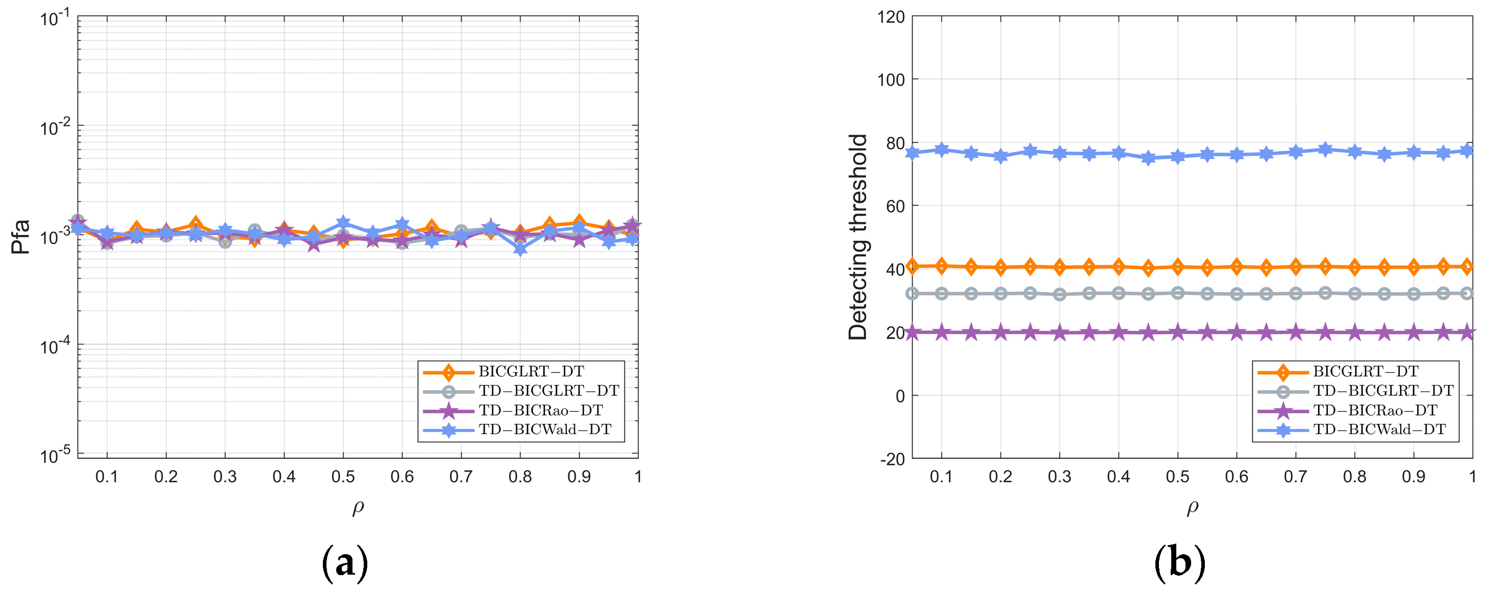
Figure 1 displays the PFA and detecting thresholds of the proposed detectors (BICGLRT-DT, TD-BICGLRT-DT, TD-BICRao-DT, and TD-BICWald-DT) versus one-lag coefficients without training data. In this case, we have ${\widehat{R}}_{MAP}=\nu \Omega /(\nu +N)$.

The above figure shows that the curves of the PFA and detecting thresholds fluctuate slowly with the change of $\rho$. Therefore, the proposed Bayesian interference-canceling detectors hold CFAR property w.r.t. the scaled matrix $\Omega$.

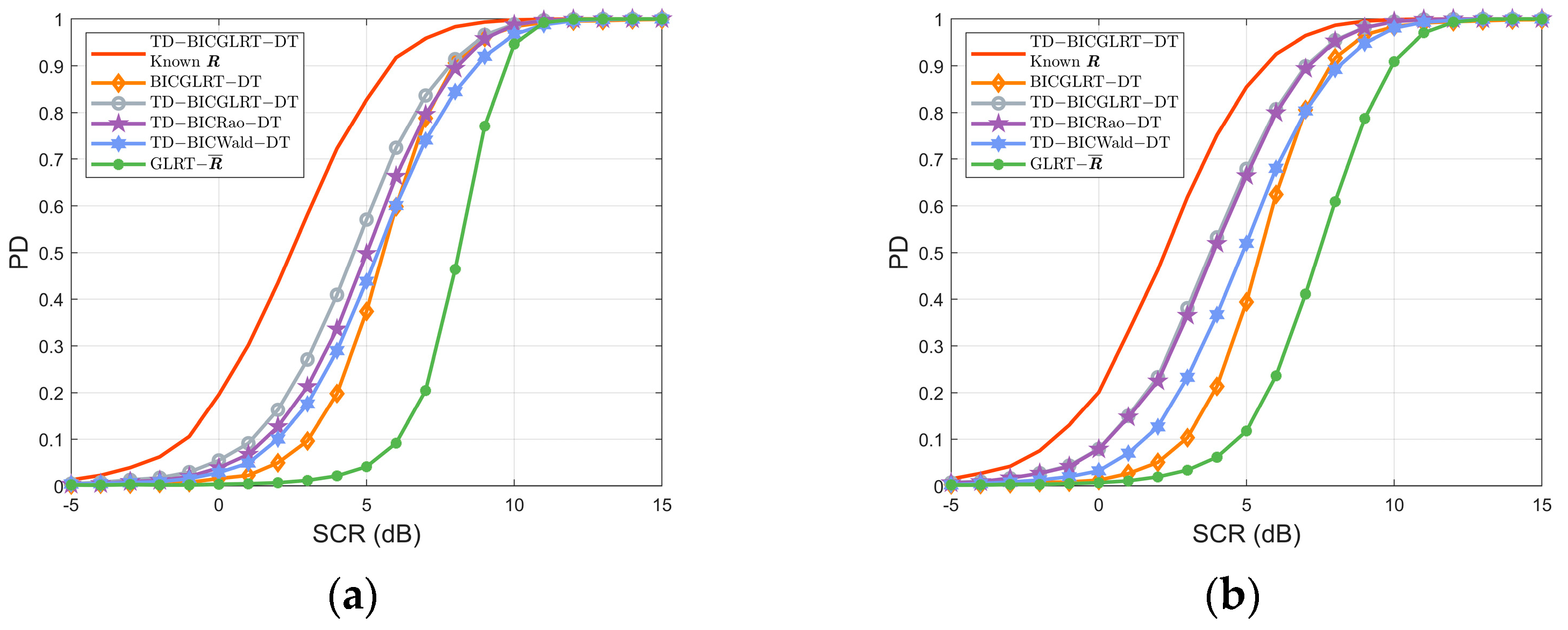
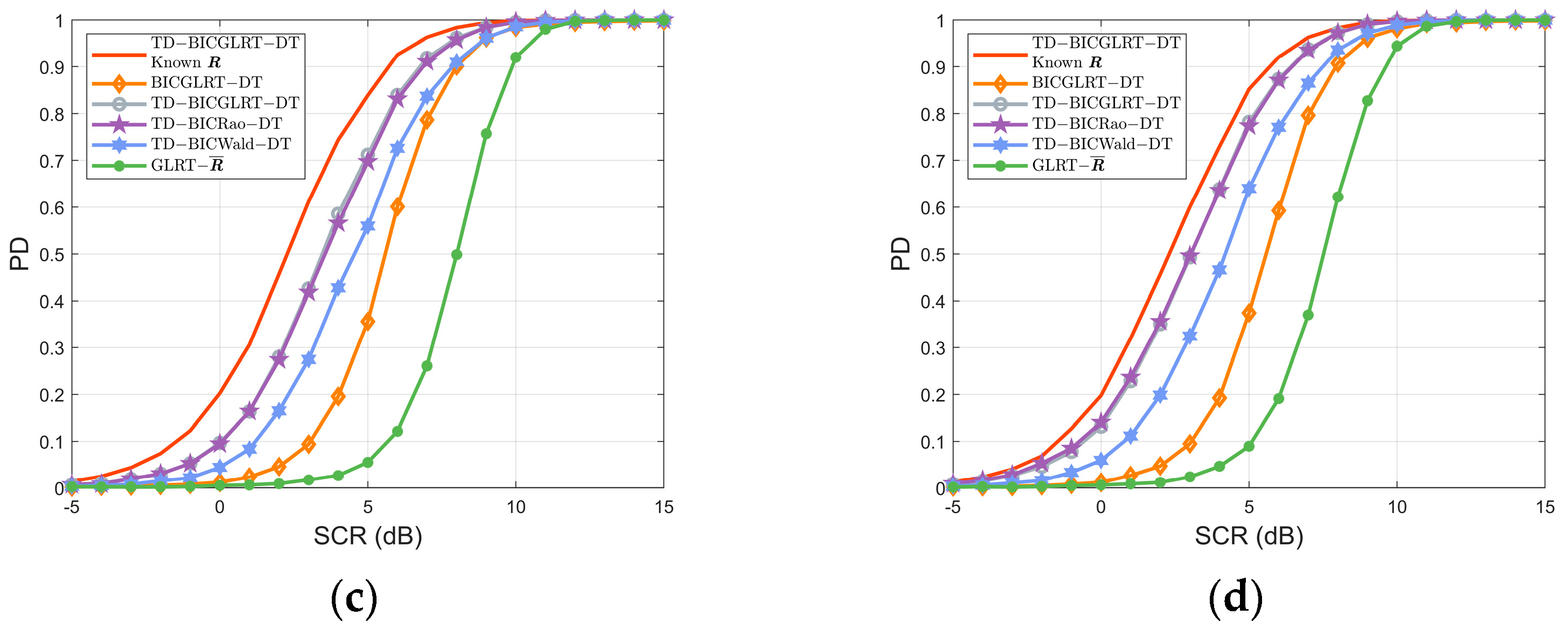
Figure 2 plots the PDs of the detectors versus SCR with the $L=6$ under different signal energy models. The curves show that the Bayesian interference-canceling detectors attain better performance than the GLRT-$\overline{R}$, the reason being that the GLRT-$\overline{R}$ does not take the existence of subspace interference into consideration. As a matter of fact, the presence of interference will raise the detecting threshold of GLRT-$\overline{R}$, therefore leading to performance degradation. By exploiting the training data, the proposed TD-BICGLRT-DT, TD-BICRao-DT, and TD-BICWald-DT outperform the BICGLRT-DT. Moreover, as discussed in Section 4, the TD-detectors achieve better performance than the BICGLRT-DT at the cost of high time complexity. Additionally, it can be seen that the TD-BICGLRT-DT has the highest PD when the signal energy is distributed uniformly. The performance of the TD-BICRao-DT degrades seriously as the signal energy gradually concentrates in a specific range cell in the CUT, indicating that the TD-BICRao-DT is sensitive to the energy distribution. In contrast, the TD-BICWald-DT is the most robust as energy distribution varies. The detailed analysis of the influence of the signal energy model can be seen in Appendix B.

In Figure 3, we investigate the detection performance of the detectors with different numbers of training data under signal energy model 1. As shown in Figure 3a, the curve of the BICGLRT-DT is nearly consistent with that of the TD-BICGLRT-DT and TD-BICRao-DT when SCR is higher than 7 dB. As $L$ gets larger, the performance of proposed TD-BICGLRT-DT, TD-BICRao-DT, and TD-BICWald-DT gradually approaches that of the TD-BICGLRT-DT with known $R$. The reason is that the increase in $L$ will make the estimated ${\widehat{R}}_{MAP}$ closer to the true $R$, therefore improving the detection performance.

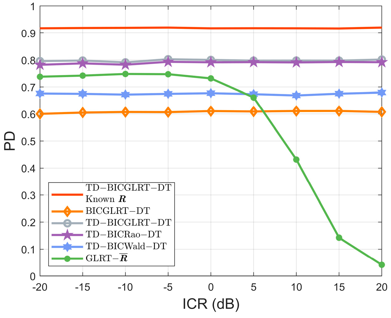
The performance comparison of the proposed BICGLRT-DT, TD-BICGLRT-DT, TD-BICRao-DT, TD-BICWald-DT, and the existing GLRT-$\overline{R}$ under different ICRs are displayed in Figure 4. As shown by the curves, the PDs of the proposed interference-canceling detectors almost stay unchanged with different ICRs, implying that the performance of the BICGLRT-DT, TD-BICGLRT-DT, TD-BICRao-DT, and TD-BICWald-DT are not influenced by the power of the subspace interference.

Figure 5 shows the PDs of the detectors when there exists a prior information mismatch. Specifically, we consider the mismatch of the one-lag coefficient $\rho$ in Figure 5a. The actual $\rho$ is set to be 0.9, and the curves indicate that the proposed detectors degrade when the presumed $\rho$ deviates from the actual $\rho$. Moreover, the TD-BICGLRT-DT, TD-BICRao-DT, and TD-BICWald-DT show better robustness than the proposed BICGLRT-DT since these three detectors utilize the training data to estimate the true $R$. 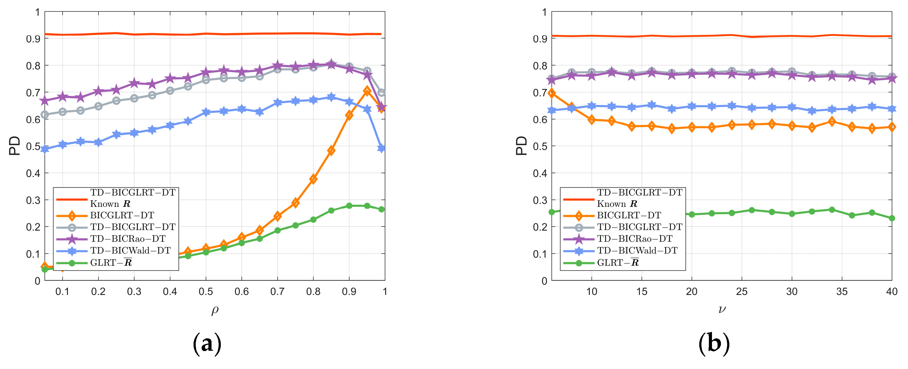In Figure 5b, we chose $\nu =15$ as the actual value of DoF. The results demonstrate that the performance of the TD-BICGLRT-DT, TD-BICRao-DT, and TD-BICWald-DT are almost not influenced by the value of actual $\nu$.

5.2. Measured Data Results

The detection performance of the Bayesian interference-canceling detectors is evaluated based on measured sea clutter data in this subsection. The sea clutter data collected by IPIX radar in 1998 is selected in this subsection [33].

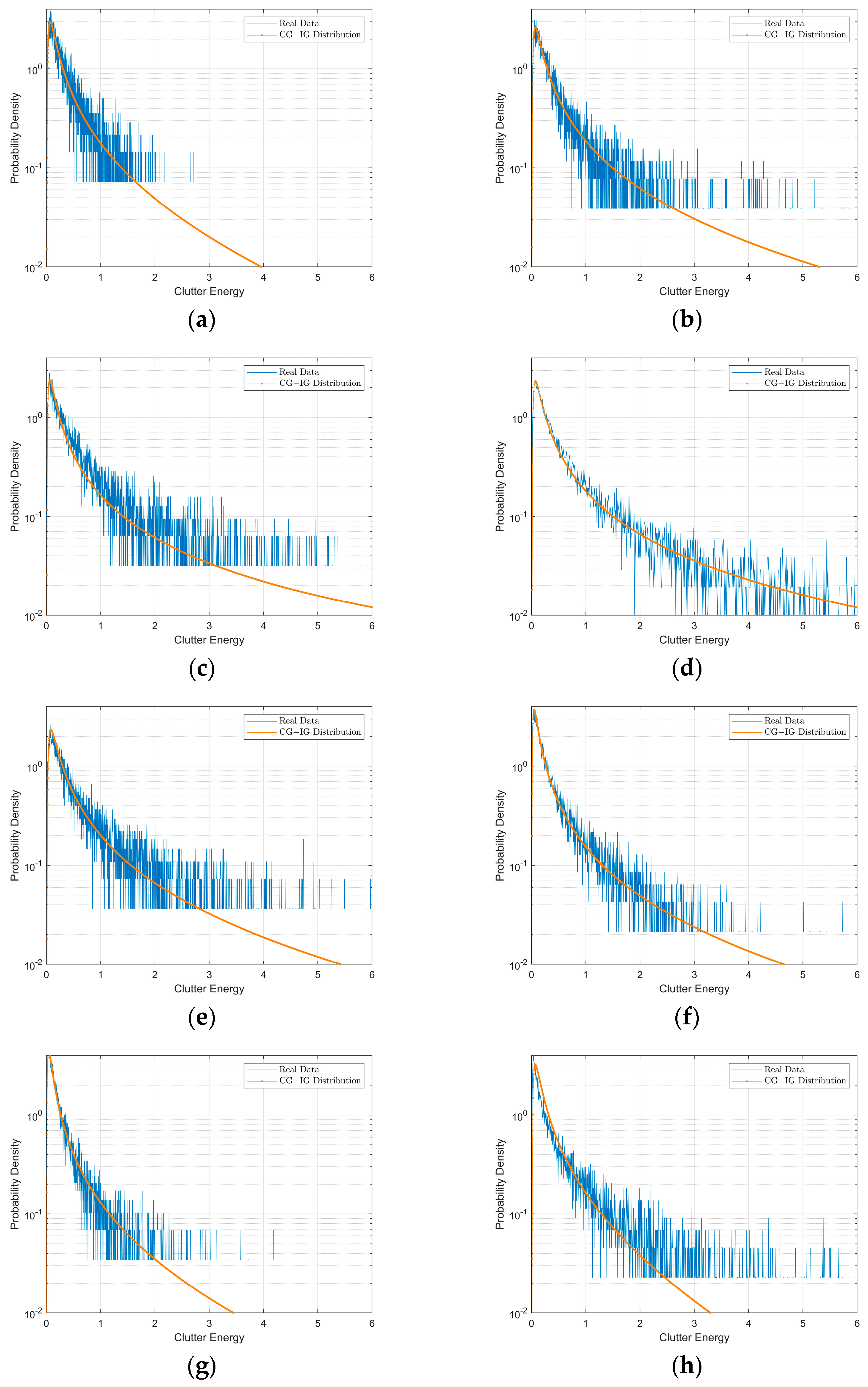
Specifically, we chose data in HH polarization in IPIX file 83 and file 84. The range–pulse spectrum of the data is shown in Figure 6. The data in file 83 and 84 contain 60,000 pulses and 34 range cells and we chose the 12th cell to the 15th cell as the CUT, meaning that $K=4$. The training data is collected from both sides of the range cells adjacent to the CUT uniformly.

To estimate the clutter shape and scale parameter, we adopt the method of fractional moments and the Nelder–Mead searching algorithm [34]. The estimated results are listed in

Table 3. Estimated parameters of the IPIX radar data.

Range Cells	$\mathit{\lambda }$	$\mathit{\mu }$
Cell 12 (File 83)	0.217	0.600
Cell 13 (File 83)	0.220	0.958
Cell 14 (File 83)	0.138	9.664
Cell 15 (File 83)	0.218	2.173
Cell 23 (File 84)	0.253	1.824
Cell 24 (File 84)	0.150	1.020
Cell 25 (File 84)	0.129	0.422
Cell 26 (File 84)	0.124	0.933

. The energy PDFs based on the measured data and estimate clutter parameter in the CUT are displayed in Figure 7.

As we can see in Figure 7, the measured clutter data can be fitted well by utilizing the IG distribution.

Due to the limited size of measured data, $P_{fa}={10}^{-2}$ is adopted. The clutter data from range cells different from CUT is utilized to estimate the scaled matrix $\Omega$ as clarified in [20].

To assess the effectiveness of our proposed Bayesian interference-canceling detectors, we add the simulated target component and subspace interference to the CUT. As shown in Figure 8, the results indicate that the Bayesian interference-canceling detectors achieve more than 5 dB SCR gain than the GLRT-$\overline{R}$ when the signal energy is distributed uniformly. As the signal energy concentrates into one specific range cell, the BICGLRT-DT, TD-BICGLRT-DT, and TD-BICWald-DT can still maintain better performance than the competitor. Thus, the measured data experiments demonstrate that the proposed interference-canceling detectors outperform the competitor in CG clutter environments with subspace interference.

6. Conclusions

The problem of Bayesian detection for distributed target under subspace interference and CG clutter with IG texture was investigated in this article. Based on the Bayesian theory, we designed six interference-canceling detectors. The first detector, named BICGLRT-DT, was constructed by eliminating the speckle CM $R$ through integration and can work without training data. Based on the two-step GLRT, complex parameter Rao, Wald, Gradient, and Durbin tests, we derived the other five detectors, which estimated the speckle CM $R$ by an iteration algorithm with limited training data. The space and time complexity of the proposed detectors were analyzed theoretically. Through the experiments, we confirmed the effectiveness of the proposed Bayesian interference-canceling detectors and pointed out the tradeoff between the time complexity and the detection performance. The experimental results based on simulated and measured sea clutter data demonstrated that the proposed TD-BICGLRT-DT, TD-BICRao-DT, and TD-BICWald-DT can achieve better performance than the proposed BICGLRT-DT since the former ones utilized the training data, leading to a higher estimate precision of $R$. Moreover, the proposed BICGLRT-DT, TD-BICGLRT-DT, and TD-BICWald-DT performed better than the existing GLRT-$\overline{R}$ with any signal energy distributions.

References

1. Xue, J.; Xu, S.; Liu, J. Persymmetric detection of radar targets in nonhomogeneous and non-Gaussian sea clutter. IEEE Trans. Geosci. Remote Sens. 2022, 60, 5103709. [Google Scholar] [CrossRef]
2. Xiao, D.; Liu, W.; Liu, J.; Dai, L.; Fang, X.; Ge, J. Adaptive radar detection of subspace-based distributed target in power heterogeneous clutter. IEEE Sens. J. 2024. [Google Scholar] [CrossRef]
3. Kelly, E.J. An adaptive detection algorithm. IEEE Trans. Aerosp. Electron. Syst. 1986, 22, 115–127. [Google Scholar] [CrossRef]
4. Conte, E.; De Maio, A. Mitigation techniques for non-Gaussian sea clutter. IEEE J. Ocean. Eng. 2004, 29, 284–302. [Google Scholar] [CrossRef]
5. Xue, J.; Liu, J.; Xu, S.; Pan, M. Adaptive detection of radar targets in heavy-tailed sea clutter with lognormal texture. IEEE Trans. Geosci. Remote Sens. 2022, 60, 5108411. [Google Scholar] [CrossRef]
6. Xue, J.; Sun, M.; Liu, J.; Xu, S.; Pan, M. Shape parameter estimation of K-distributed sea clutter using neural network and multisample percentile in radar industry. IEEE Trans. Ind. Informat. 2023, 19, 7602–7612. [Google Scholar] [CrossRef]
7. Carretero-Moya, J.; Gismero-Menoyo, J.; Blanco-del-Campo, Á.; Asensio-Lopez, A. Statistical analysis of a high-resolution seaclutter database. IEEE Trans. Geosci. Remote Sens. 2010, 48, 2024–2037. [Google Scholar] [CrossRef]
8. Xue, J.; Xu, S.; Liu, J.; Shui, P. Model for non-Gaussian sea clutter amplitudes using generalized inverse Gaussian texture. IEEE Geosci. Remote Sens. Lett. 2018, 16, 892–896. [Google Scholar] [CrossRef]
9. Reed, I.S.; Mallett, J.D.; Brennan, L.E. Rapid convergence rate in adaptive arrays. IEEE Trans. Aerosp. Electron. Syst. 1974, AES-10, 853–863. [Google Scholar]
10. Conte, E.; Lops, M.; Ricci, G. Adaptive matched filter detection in spherically invariant noise. IEEE Signal Process. Lett. 1996, 3, 248–250. [Google Scholar] [CrossRef]
11. Conte, E.; De Maio, A.; Ricci, G. Recursive estimation of the covariance matrix of a compound-Gaussian process and its application to adaptive CFAR detection. IEEE Trans. Signal Process. 2002, 50, 1908–1915. [Google Scholar] [CrossRef]
12. Coluccia, A.; Fascista, A.; Orlando, D.; Ricci, G. Adaptive radar detection in heterogeneous clutter plus thermal noise via the expectation-maximization algorithm. IEEE Trans. Aerosp. Electron. Syst. 2024, 60, 212–225. [Google Scholar] [CrossRef]
13. Ye, H.; Wang, Y.L.; Liu, W.; Liu, J.; Chen, H. Adaptive detection in partially homogeneous environment with limited samples based on geometric barycenters. IEEE Signal Process. Lett. 2022, 29, 2083–2087. [Google Scholar] [CrossRef]
14. Cao, Z.; Cui, N.; Xing, K.; Liu, W.; Yu, Z. Low-complexity subarray-based adaptive detection for multichannel application in inhomogeneous clutter environments. IEEE Geosci. Remote Sens. Lett. 2024, 21, 3500405. [Google Scholar] [CrossRef]
15. Elias, A.; Bernard, M. Hybrid detection approach for STAP in heterogeneous clutter. IEEE Trans. Aerosp. Electron. Syst. 2010, 46, 1021–1033. [Google Scholar]
16. Aubry, A.; De Maio, A.; Pallotta, L. A geometric approach to covariance matrix estimation and its application to radar problems. IEEE Trans. Signal Process. 2018, 66, 907–922. [Google Scholar] [CrossRef]
17. Besson, O.; Tourneret, J.Y.; Bidon, S. Knowledge-aided Bayesian detection in heterogeneous environments. IEEE Signal Process. Lett. 2007, 14, 355–358. [Google Scholar] [CrossRef]
18. Svensson, L.; Lundberg, M. On posterior distributions for signals in Gaussian noise with unknown covariance matrix. IEEE Trans. Signal Process. 2005, 53, 3554–3571. [Google Scholar] [CrossRef]
19. Bandiera, F.; Besson, O.; Ricci, G. Adaptive detection of distributed-targets in compound-Gaussian noise without secondary data: A Bayesian approach. IEEE Trans. Signal Process. 2011, 59, 5698–5708. [Google Scholar] [CrossRef]
20. Xue, J.; Xu, S.; Shui, P.L. Knowledge-based target detection in compound Gaussian clutter with inverse Gaussian texture. Digit. Signal Process. 2019, 95, 102590. [Google Scholar] [CrossRef]
21. Guo, H.; Wang, Z.; Wu, H.; He, Z.; Cheng, Z. Bayesian detection for distributed targets in compound Gaussian sea clutter with lognormal texture. Signal Process. 2025, 227, 109751. [Google Scholar] [CrossRef]
22. Bandiera, F.; Ricci, G. Adaptive detection and interference rejection of multiple point-like radar targets. IEEE Trans. Signal Process. 2006, 54, 4510–4518. [Google Scholar] [CrossRef]
23. Besson, O. Detection in the presence of surprise or undernulled interference. IEEE Signal Process. Lett. 2007, 14, 352–354. [Google Scholar] [CrossRef]
24. Sun, M.; Liu, W.; Liu, J.; Tang, P.; Hao, C. Adaptive subspace detection based on Gradient test for orthogonal interference. IEEE Trans. Aerosp. Electron. Syst. 2022, 58, 1868–1877. [Google Scholar] [CrossRef]
25. Yan, L.; Addabbo, P.; Hao, C.; Orlando, D.; Farina, A. New ECCM techniques against noiselike and/pr coherent interferers. IEEE Trans. Aerosp. Electron. Syst. 2020, 56, 1172–1188. [Google Scholar] [CrossRef]
26. Mezache, A.; Soltani, F.; Sahed, M.; Chalabi, I. Model for non-Rayleith clutter amplitudes using compound inverse Gaussian distribution: An experimental analysis. IEEE Trans. Aerosp. Electron. Syst. 2015, 51, 142–153. [Google Scholar] [CrossRef]
27. Tague, J.A.; Caldwell, C.I. Expectations of useful complex Wishart forms. Multidimens. Syst. Signal Process. 1994, 5, 263–279. [Google Scholar] [CrossRef]
28. Roper, L.D. Numerical recipes: The art of scientific computing. Bull. Math. Biol. 1987, 49, 761–762. [Google Scholar]
29. Robey, F.C.; Fuhrmann, D.R.; Kelly, E.J.; Nitzberg, R. A CFAR adaptive matched filter detector. IEEE Trans. Aerosp. Electron. Syst. 1992, 28, 208–216. [Google Scholar] [CrossRef]
30. Liu, W.; Liu, J.; Hao, C.; Gao, Y.; Wang, Y.L. Multichannel adaptive signal detection: Basic theory and literature review. Sci. China Inf. Sci. 2022, 65, 121301. [Google Scholar] [CrossRef]
31. Sun, M.; Liu, W.; Liu, J.; Hao, C. Complex parameter Rao, Wald, Gradient and Durbin tests for multichannel signal detection. IEEE Trans. Signal Process. 2022, 70, 117–131. [Google Scholar] [CrossRef]
32. Conte, E.; De Maio, A. Distributed target detection in compound-Gaussian noise with Rao and Wald tests. IEEE Trans. Aerosp. Electron. Syst. 2003, 39, 568–582. [Google Scholar] [CrossRef]
33. The McMaster IPIX Radar Sea Clutter Database. Available online: http://soma.mcmaster.ca/ipix.php (accessed on 1 July 2001).
34. Mezache, A.; Sahed, M.; Laroussi, T. K-distribution parameters estimation based on the Nelder-Mead algorithm in presence of thermal noise. In Proceedings of the International Conference on Advances in Computational Tools for Engineering Applications, Beirut, Lebanon, 15–17 July 2009. [Google Scholar]
Figure 1. PFA and threshold curves of the proposed interference-canceling detectors: (a) P f a versus ρ ; (b) Detecting threshold versus ρ .
Remotesensing 17 00926 g001
Figure 2. PDs of the detectors under different signal energy models with L = 6 : (a) Model 1; (b) Model 2; (c) Model 3; (d) Model 4; (e) Model 5; (f) Model 6.
Remotesensing 17 00926 g002aRemotesensing 17 00926 g002b
Figure 3. Detection performance of the detectors under different number of training data with signal energy model 1: (a) L = 0 ; (b) L = 6 (c) L = 12 ; (d) L = 24 .
Remotesensing 17 00926 g003aRemotesensing 17 00926 g003b
Figure 4. PDs of the detectors under different ICRs with SCR = 6 dB and L = 6 .
Remotesensing 17 00926 g004
Figure 5. PDs of the detectors in the presence of prior information mismatch with L = 6 . (a) different ρ with actual ρ = 0.9 ; (b) different ν with actual ν = 15 .
Remotesensing 17 00926 g005
Figure 6. Range-pulse spectrum of the selected data. (a) File 83; (b) File 84.
Remotesensing 17 00926 g006
Figure 7. Energy probability density functions based on measure data and estimated parameters: (a) cell 12 (File 83); (b) cell 13 (File 83); (c) cell 14 (File 83); (d) cell 15 (File 83); (e) cell 23 (File 84); (f) cell 24 (File 84); (g) cell 25 (File 84); (h) cell 26 (File 84).
Remotesensing 17 00926 g007
Figure 8. PDs of the detectors under different signal energy models with L = 6 based on measure data: (a) Model 1 (File 83); (b) Model 6 (File 83); (c) Model 1 (File 84); (d) Model 6 (File 84).
Remotesensing 17 00926 g008