Abstract
Transformers have performed favorably in recent hyperspectral unmixing studies in which the self-attention mechanism possesses the ability to retain spectral information and spatial details. However, the lack of reliable prior information for correction guidance has resulted in an inadequate accuracy and robustness of the network. To benefit from the advantages of the Transformer architecture and to improve the interpretability and robustness of the network, a dual-branch network with prior information correction, incorporating a Transformer network (PICT-Net), is proposed. The upper branch utilizes pre-extracted endmembers to provide pure pixel prior information. The lower branch employs a Transformer structure for feature extraction and unmixing processing. A weight-sharing strategy is employed between the two branches to facilitate information sharing. The deep integration of prior knowledge into the Transformer architecture effectively reduces endmember variability in hyperspectral unmixing and enhances the model’s generalization capability and accuracy across diverse scenarios. Experimental results from experiments conducted on four real datasets demonstrate the effectiveness and superiority of the proposed model.
1. Introduction
Hyperspectral imaging (HSI), a representative technology used in Earth sciences and remote sensing [1], has attracted increasing attention for hyperspectral data processing and analysis.
Hyperspectral unmixing (HU) is a crucial preprocessing technique in spectral data analysis, designed to identify the constituent components (endmembers) and determine the proportion (abundance) of each component within the HSI. Currently, HU is mainly performed based on linear mixing models, and nonlinear mixing models. However, in HSI, spectral variabilities (SV) might consist of scaling factors caused by illumination and topography changes, complex noise from environmental conditions or instrumental sensors, physical and chemical atmospheric effects, and the nonlinear mixing of materials [2]. Thus, simple linear models cannot fully fit the complicated spectral mixing phenomena. Therefore, it is critical to investigate the nonlinear model of HU.
The powerful nonlinear fitting capability of deep learning has been applied in the field of HU. Su [3] developed a new unsupervised unmixing technique based on a deep autoencoder (AE) network. In [4], a novel endmember extraction and HU scheme utilizing a two-stage AE network was proposed, demonstrating superior unmixing results. B. Palsson [5] proposed a new spectral–spatial linear mixing model and a correlation estimation method based on convolutional neural network (CNN) AE unmixing, which exhibited a good performance and consistency in terms of endmember extraction. In [6], a novel deep blind HU scheme based on a deep AE network was developed, which only relies on the current data, and does not require additional training. Gao [7] proposed a cycle-consistent unmixing network called CyCU-Net, which learns from two cascaded AEs in an end-to-end manner to improve the unmixing performance more effectively. V.S.S [8] proposed a two-stage fully connected self-supervised deep learning network to address these practical challenges in blind hyperspectral unmixing, whose inverse model is based on an AE network. It effectively handles the high implicit noise present in the data. In some cases, network models based on AEs might produce endmembers that do not always have a direct physical interpretation in real-world scenarios.
The self-attention mechanism in the Transformer can preserve spectral information, spatial details, and has the ability to capture global contextual feature dependencies, which is suitable for HSI unmixing [9]. As a deep learning network that pays more attention to global information, Transformer has been favored by researchers over the past few years. P. Ghosh [10] proposed a deep unmixing model with a combination of a convolutional AE and a Transformer, which utilizes the ability of the Transformer to capture global feature dependencies better and improves the quality of the endmember and abundance maps. Duan [11] proposed a novel unmixing-guided convolutional Transformer (UGCT) network that achieves a finer interpretation of HSI mixed pixels and shows an improved reconstruction performance. F. Kong [12] applied a well-designed Transformer encoder for HU before a CNN to explore nonlocal information through an attention mechanism called window-based pixel-level multi-head self-attention (MSA). In [13], a novel dual-aware Transformer network, UnDAT, for HU was proposed to utilize both the regional homogeneity and spectral correlation of hyperspectral images. In [14], a U-shaped Transformer network using shifted windows prioritized more discriminative and salient spatial information in a scene using multiple self-attentive blocks. Fazal [15] proposed a new approach for HU using a deep convolutional Transformer network that combines a CNN-based AE with a Transformer and extracts low-level features from the input image to obtain better unmixing results. A new method, shifted-window (Swin) HU, based on the Swin Transformer, was proposed in [16], aiming to solve the blind HU problem effectively. In 2024, Wang Li et al. [17] proposed a HyperGAN network model based on the Transformer architecture. The former completes the modal conversion of the mixed hyperspectral pixel patch to the corresponding end of the central pixel, while the latter is used to distinguish whether the generated abundant distribution and structure are the same as the real one, and good test results have been obtained. In [18], a new Transformer-based model for unmixing the mixed pixel, named Convolutional Vision Transformer-based Hyperspectral Unmixing (CvTHU), was proposed. The dimensionality of the hyperspectral image is reduced using a combination of PCA and hybrid spectral–spatial feature extraction using a 3D–2D Convolutional Neural Network, and the unmixing of the hyperspectral image is performed using the Convolutional Vision Transformer (CvT), which improved the performance without increasing the computational complexity compared to the Vision Transformer-based unmixing. Reference [19] explores a dual-stream collaborative network, referred to as TCCU-Net. It end-to-end learns information in four dimensions, spectral, spatial, global, and local, to achieve more effective unmixing. Xu Cheng et al. [20] propose a multiscale visual transformer network using a convolution crossing attention (CCA) (MSCC-ViT) model, which aims to extract feature information from hyperspectral images (HSI) at different scales and effectively fuse them, allowing the model to simultaneously recognize parts of the HSI with similar spectral features and distinguish parts with different features. Yang Yuanhu et al. [21] present a cascaded dual-constrained transformer autoencoder (AE) for HU with endmember variability and spectral geometry. The model utilizes a transformer AE network to extract the global spatial features from the HSI. Additionally, it incorporates the minimum distance constraint to account for the geometric information of the HSI. Ge Youran et al. [22] propose an innovative AE named Transformer-enhanced convolutional neural network (CNN) based on intensive features (TCN), which is based on a spatial–spectral decomposition fusion mechanism and integrates the local modeling capability of the CNN with the global context modeling capability of Transformer to improve the performance of HU. Reference [23] proposes a multiscale aggregation Transformer network (MAT-Net), which utilizes an encoder–decoder architecture designed to harness both spectral and spatial data comprehensively. However, when the spectral pixels are highly mixed, the network unmixing results are not ideal and abundance maps with good effects cannot be obtained because they lack the corrective guidance of reliable prior knowledge.
The guidance of real endmembers is equivalent to adding prior spectral knowledge, which can correct the unmixing results to a certain extent and achieve the goal of improving the unmixing accuracy. Based on this, EGU-Net has been proposed in [2], which uses real endmembers to guide the network and indeed achieves the purpose of improving the unmixing accuracy. In [24], context information within the HSI space is utilized as prior knowledge to compute abundances during sparse unmixing operations, resulting in a favorable performance under varying noise conditions, particularly in scenarios with low signal-to-noise ratios. Meng Fanlei et al. [25] proposed an efficient coupled transformer network for robust hyperspectral unmixing called CTNet, which incorporate a two-stream half-Siamese network with an additional encoder trained on pseudo-pure pixels, and further integrates a cross-attention module to leverage global information. Therefore, the extraction of a priori knowledge from the original HSI should be used to correct and guide the network unmixing results. Reference [26] proposed a method to capture effective prior information about endmember signatures and abundance distributions, integrating these as valuable constraints into NMF to enhance the model’s unmixing performance.
Based on the advantages of the Transformer network structure and the idea of adding prior knowledge, it is proposed to use the prior knowledge extracted from the original HSI to correct and guide the network unmixing results to solve the above problems. Compared to existing work, the proposed model shows distinct advantages. Typical unmixing network models that incorporate prior knowledge fail to model global information dependencies, while models capable of capturing long-range dependencies often struggle with a weak suppression of endmember variability. Our proposed model addresses both issues simultaneously and leads to an improved generalization performance.
In order to enhance unmixing network correction, the incorporation of prior knowledge through a Transformer network (PICT-Net) is proposed. PICT-Net adopts a dual-stream network structure for HSI unmixing, where the upper branch network obtains reliable network weights by learning pure pixel blocks, and corrects the results of the network for HSI unmixing through the shared weights strategy, thus improving the unmixing accuracy. The main contributions of this study are summarized as follows.
- A dual-branch network incorporating a Transformer with prior information correction is proposed. It improves the accuracy of the network in a more reliable and generalizable way.
- A hyperspectral feature extraction module that combines CNN and pooling operations to avoid losing important features and details during the dimensionality reduction process is designed.
- A weight-sharing strategy based on Transformer was designed. The query vector () was selected for sharing to ensure the reasonableness of the strategy.
A graphical representation of the proposed Transformer-based hyperspectral unmixing framework is shown in Figure 1.
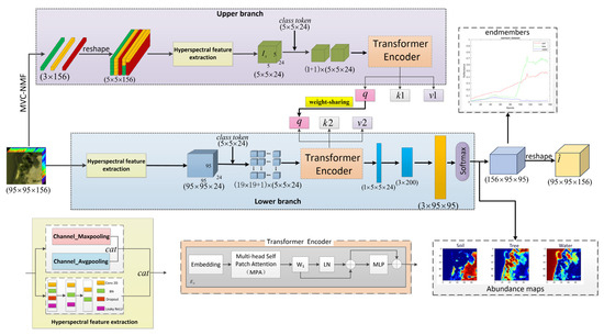
Figure 1.
Graphical representation of the proposed Transformer-based hyperspectral unmixing framework (PICT-Net).
2. Materials and Methods
Let the spatial dimension of the original hyperspectral image I be and the size of the spectral dimension be B. The parameter denotes the number of endmembers.
2.1. Upper Branch Network Structure
2.1.1. Extraction of Pseudo-Pure Pixel Blocks
An analysis of classical endmember extraction algorithms [27] (Ersen, Li et al., 2011) showed that the MVC-NMF algorithm has the most precise endmember extraction results. To improve the robustness of blind unmixing and enhance the interpretability of the network structure, pseudo-pure spectral pixel blocks were obtained from the original image by MVC-NMF endmember extraction algorithms. The matrix results obtained using MVC-NMF were copied and reshaped by MATLAB R2022b to obtain a pseudo-pure pixel block that was proportional to the dimension of the original HSI. The dimensions of the obtained pseudo-pure pixel block are , which are fed into the upstream network to obtain the network parameters with reference guidance significance as a priori knowledge to correct the blind unmixing of the original HSI.
2.1.2. Hyperspectral Feature Extraction with Pooling
Hyperspectral images have huge data redundancy in the spectral dimension. According to previous experiments, applying dimensionality reduction steps before deep learning can significantly improve model performance [28] (B. Rasti et al., 2022). The channel maximum pooling operation is performed on the input to reduce the computational complexity of the model and retain the maximum features while dimensionality reduction is achieved. Meanwhile, the average pooling operation is carried out to reduce information loss during dimensionality reduction. At the same time, to ensure that spatial information is not lost, a three-layer convolution operation is employed. The convolution operation uses a kernel size of 1 × 1 to prevent excessive model parameters. All layers use batch normalization (BN) after the two-dimensional (2D) convolution operation, the dropout function in the first layer to mitigate the problem of the vanishing gradient of the network and the Leaky ReLU function in the output of the first two layers to introduce nonlinearity. Then, the results of the two pooling operations and the three-layer convolution operation in the channel dimension are concatenated. After that, the spectral dimension was reduced to C by a convolution operation with a kernel size of 1 × 1. C is the hyperparameter being defined.
2.1.3. Transformer Encoder
To effectively capture the correlation of long-range features, the outputs of the upper and lower stream encoders were arranged in chunks, and the outputs of the upper and lower stream encoders were the cube with dimension () and the cube with dimension (), where refer to the spatial dimensionality, and C denotes the number of spectral channels that go through the outputs of the CNN layer, respectively. These features are divided into multiple patch tokens, each with a dimension sizes of , which means that is the spatial dimension size of a patch token and its spectral channel number is C. Therefore, the cube is divided into according to the formula , where is the total number of patch tokens contained in the cube. In the next step, a learnable vector class token of dimension is defined because the transformer encoder will capture long-range semantic information for the patch tokens in this vector and it is attached to the partitioned cube matrix patch token. At this time, the dimension size of this cube matrix becomes . Afterward, for the model to better understand the relative positional relationship between different patches, positional embedding is performed for each patch to obtain matrix X.
Next, matrix goes through layer normalization and enters the Transformer encoder to undergo a multi-head self-attention computation, the purpose of which is to exchange information within the patch token to capture its remote context information and input it into the class token.
Attention is mainly computed with three weight parameters, , where represents the query vector of the current element; is the key vector, which represents the keyword vector of all the elements; and denotes the value vector of all the elements. The three parameters are obtained from three linear variations, in which is obtained from the class token through the weight matrix , and and are obtained from the patch token through the weight matrices and .
The setting of the upper branch is chosen to obtain reliable parameters in the encoder; the subsequent steps are the same as those used for the lower branch but as this is not the focus of this study, these will not be repeated here, and the specific terms used here can also refer to the description of the lower branch.
2.2. Weight Sharing Strategy
To introduce prior knowledge for corrective guidance of the unmixing results, a weight-sharing strategy was designed. The attention mechanism assigns weights based on the similarity between the query and the key. In the actual calculation process, come entirely from the original image, focusing on the contextual information within the image itself. The top-end flow network selects pseudo-pure spectral pixel blocks from the original image, so that does not include reliable contextual information. Therefore, the weights will not be shared. The weight is derived from learnable class tokens, whose purpose is to incorporate category information into the computation of the attention mechanism; thereby, the weight learned from provides reliable contextual information about the category. To ensure the rationality of the parameter-sharing strategy, only weight is shared to prevent the network from generating physically meaningless endmembers, which reduce the accuracy of subsequent HU results, and to produce correct and reliable abundance estimates.
2.3. Lower-End Flow Network Structure
The original HSI is used as the input to the lower-end flow network, which contains HS feature extraction, a Transformer encoder, decoder, and loss and optimization functions.
In part A of this section, HS feature extraction and the calculation of parameters was discussed. The other features will be discussed below.
2.3.1. Transformer Encoder
A multi-head attention (MHA) mechanism is used to enhance the connection of information between different patches of HSI for better global information interaction. To this end, the parameter dimension is reshaped to , where is the number of heads, to obtain . Similarly, the size of is reshaped to obtain . Attention weights are obtained by calculating the similarity between weights and , and then mapping them into the range [0, 1] using the SoftMax function. To prevent the problem of the gradient of the SoftMax function being too small, the attention weight is scaled by . The attention weight matrix is multiplied by the value vector to obtain the multi-head patch self-attention (MPA). The MPA is expressed in Equation (4).
Next, the attention size is reshaped into a matrix of size (1 × ). The attention matrix is passed through a linear layer and summed with the class token to obtain the classification output .
The output is then concatenated with the layer-normalized (LN) patch token matrix.
The matrix is passed through the normalization layer and fed into an MLP along with a residual connection to obtain the final output of the Transformer encoder.
2.3.2. Decoder
The encoder produces the result with the size . The size is reshaped to , where represents the number of endmembers in the dataset. In the next step, the dimensions are expanded by up sampling to . A convolution operation with a kernel size of 3 × 3 is used to obtain an abundance cube R with the size .
The result needs to satisfy the abundance sum-to-one (ASC) constraint and the abundance non-negative (ANC) constraint. Thus, the SoftMax function was utilized in the spectral channel so that these constraints can be satisfied. In the next step, a convolution operation with a kernel size of 1 × 1 was performed to expand the number of spectral channels from to B to obtain the reconstructed HSI. The weights of the convolutional layer were initialized by the MVC-NMF and optimized to estimate the endmember.
2.3.3. Loss and Optimization Functions
The following two loss metrics were used to optimize the network: reconstruction error (RE) loss and spectral angular distance (SAD) loss.
The RE loss is sensitive to the spectral magnitude. Its gradient direction tends to reduce the global numerical error rapidly. At the same time, the SAD loss is sensitive to the spectral shape, and its gradient direction focuses on adjusting the orientation of the spectral curve. The gradient directions of these two losses are complementary, and their weighted sum provides a more comprehensive optimization signal, reducing oscillations and converging faster.
Here, and are regularization parameters, which are manually tuned.
3. Experiments
3.1. Description of Datasets
In this section, we present the performance of the proposed method on the real Samson, Apex, Houston, and muffle datasets.
3.1.1. Samson Dataset
This dataset contains 95 × 95 hyperspectral pixels. Each hyperspectral pixel contains reflectance values in 156 bands, covering the wavelength range of [401–889] nm, and contains three endmembers: “soil”, “tree” and “water”, which is shown in Figure 2.
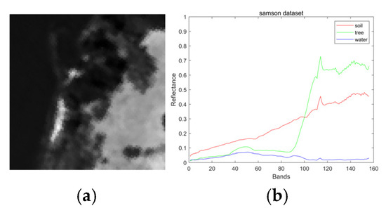
Figure 2.
(a) Samson dataset grayscale. (b) Samson dataset endmembers.
3.1.2. Apex Dataset
The images contain 110 × 110 hyperspectral pixels. Each hyperspectral pixel contains reflectance values in 285 bands covering a wavelength range of [413–2420] nm. The hyperspectral image has four endmembers, “water”, “tree”, “road” and “roof”, which is shown in Figure 3.
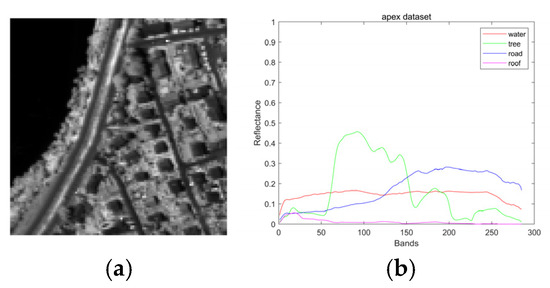
Figure 3.
(a) Apex dataset grayscale. (b) Apex dataset endmembers.
3.1.3. Houston Dataset
We investigate a 170 × 170 pixels subimage cropped from the original image. Each hyperspectral pixel contains reflectance values in 144 bands covering a wavelength range of [364–1046] nm. The hyperspectral image has four endmembers: “Stadium seats”, “Parking lot”, “Building facility” and “grass”, which is shown in Figure 4.
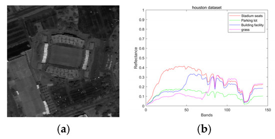
Figure 4.
(a) Houston dataset grayscale. (b) Houston dataset endmembers.
3.1.4. Muffle Dataset
The images contain 90 × 90 hyperspectral pixels. Each hyperspectral pixel contains reflectance values in 64 bands covering a wavelength range of [375–1050] nm. The hyperspectral image has five endmembers: “roof”, “grass”, “tree”, “asphalt” and “shadow”, which is shown in Figure 5.
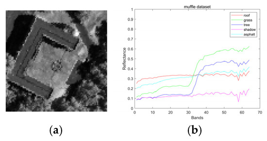
Figure 5.
(a) Muffle dataset grayscale. (b) Muffle dataset endmembers.
3.2. Hyperparameter Setting
Hyperparameters play a particularly important role in the training process and unmixing results of the model, and choosing appropriate hyperparameters can significantly improve model performance. The hyperparameter settings for the different datasets are as follows.
3.2.1. Samson Hyperspectral Dataset
The size of the patch token was selected to be (), the spectral dimension of the input transformer encoder was selected to be 24 and the regularization parameters were taken as 6.5 × 10⁴ and , respectively. In this model, the task was completed for 200 iterations, where the initial learning rate was set to . The learning rate decreased by 20% every 15 iterations, and the weight decay rate was added after the loss function to control the complexity of the model and avoid the overfitting problem.
3.2.2. Apex Hyperspectral Dataset
The size of the patch token was chosen to be (), the spectral dimension of the input transformer encoder was chosen to be 32 and the regularization parameters were taken as and , respectively. In this model, 200 iterations of the task were completed, in which the initial learning rate was set to , and the learning rate decreased by 20% every 15 iterations. A weight decay rate of was added after the loss function to control the complexity of the model and avoid the overfitting problem.
3.2.3. Houston Hyperspectral Dataset
The size of the patch token was chosen to be (), the spectral dimension of the input transformer encoder was chosen to be 40 and the regularization parameters were taken as and , respectively. In this model, 200 iterations of the task were completed, in which the initial learning rate was set to , and the learning rate decreased by 20% every 15 iterations. A weight decay rate of was added after the loss function to control the complexity of the model and avoid the overfitting problem.
3.2.4. Muffle Hyperspectral Dataset
The size of the patch token was chosen to be (), the spectral dimension of the input transformer encoder was chosen to be 32 and the regularization parameters were taken as and , respectively. In this model, 200 iterations of the task were completed, in which the initial learning rate was set to , and the learning rate decreased by 20% every 15 iterations. A weight decay rate of was added after the loss function to control the complexity of the model and avoid the overfitting problem.
Basic information and optimal hyperparameters were determined through experiments, as shown in Table 1 for the different datasets.

Table 1.
Basic information on experimental datasets and hyperparameter settings for training.
3.3. Evaluation Metrics
The unmixing performance was evaluated by collecting all pixel abundances to calculate the overall root mean square error (RMSE) of abundance, which describes the difference between the estimated and true values of elemental abundance, and is defined as shown in Equation (11):
where is the true value of elemental abundance and is the estimated value of elemental abundance.
The aSAD describes the similarity between the spectral features of the original endmembers and their estimated values. The smaller the aSAD value, the more similar the spectral features of the original endmembers are to the estimated value, which proves that the experimental results are better. The specific definitions are as follows:
where denotes the column of the true endmember matrix S, and is the column of the estimated endmember matrix .
3.4. Results
Four unmixing methods proposed in recent years were compared: a cycle-consistent unmixing network (CyCU-Net) [7], an endmember-guided unmixing network (EGU-Net) [2], a deep unmixing model combining a convolutional AE and a Transformer network (DeepTrans) [10] and a shifted-window (Swin) HU based on the Swin Transformer network (Swin-HU) [16]. CyCU-Net learns from two cascaded AEs in an end-to-end manner to improve HU performance. EGU-Net uses real endmembers to guide the network. DeepTrans applies the Transformer to HU, and Swin-HU utilizes a more advanced Transformer network for HU.
Root mean square error (RMSE) and the average spectral angle distance (aSAD) were used to evaluate model performance. The results confirm that the proposed model performs better than the other methods. The results for the RMSE values of the different HU methods (CyCU-Net, EGU, DeepTrans, SwinHU and PICT-Net) on four different real datasets(Samosn, Apex, Houston and muffle) are shown in Table 2.
Table 2.
RMSE of different HU methods (CyCU-Net, EGU, DeepTrans, SwinHU, and PICT-Net) on 4 different real datasets(Samosn, Apex, Houston and muffle). The best performances are shown in bold.
The results for the aSAD of the different HU methods (CyCU-Net, EGU, DeepTrans, SwinHU and PICT-Net) on four different real datasets (Samosn, Apex, Houston and muffle) are sown in Table 3, which shows that the proposed model performs better than other methods.
Table 3.
aSAD of different HU methods (CyCU-Net, EGU, DeepTrans, SwinHU and PICT-Net) on 4 different real datasets (Samosn, Apex, Houston and muffle). The best performances are shown in bold.
Figure 6 and Figure 7 show the abundance maps and endmember spectra obtained by the different unmixing methods on the Samson dataset, respectively.
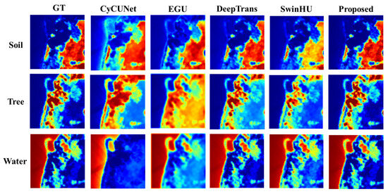
Figure 6.
Ground truth and extracted abundance maps for Samson dataset using different HU methods (CyCU-Net, EGU, DeepTrans, SwinHU and PICT-Net). The colors represent the abundance values from blue (sk = 0) to red (sk = 1).
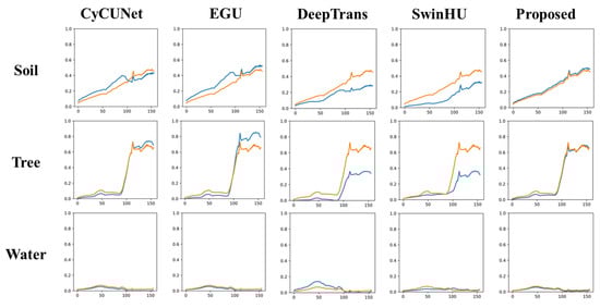
Figure 7.
Ground truth endmember spectra and extracted endmember spectra for the Samson dataset using different HU methods (CyCU-Net, EGU, DeepTrans, SwinHU and PICT-Net). The yellow line is the ground truth, and the blue line represents the endmembers estimated by the HU methods.
As can be seen, the proposed method can extract the exact abundance maps and endmember signatures. PICT-Net outperforms other methods for extracting the endmembers and their corresponding abundances from the Samson dataset.
The visualized unmixing results of the abundance maps and endmembers for the Apex dataset are shown in Figure 8 and Figure 9, respectively.
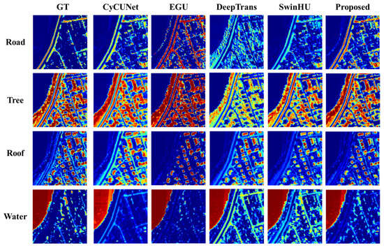
Figure 8.
Ground truth and extracted abundance maps for Apex dataset using different HU methods (CyCU-Net, EGU, DeepTrans, SwinHU, and PICT-Net). The colors represent the abundance values from blue (sk = 0) to red (sk = 1).
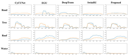
Figure 9.
Ground truth endmember spectra and extracted endmember spectra of the Apex dataset using different HU methods (CyCU-Net, EGU, DeepTrans, SwinHU and PICT-Net). The yellow line is the ground truth, and the blue line represents the endmembers estimated by the HU methods.
The abundance maps and endmembers generated by different methods on the Apex dataset indicate that PICT-Net is better able to learn detailed information, and the endmembers fit better.
Figure 10, Figure 11, Figure 12 and Figure 13 below illustrate the abundance maps and endmember performances generated by the proposed model compared to the other four methods (CyCU-Net, EGU, DeepTrans and SwinHU) on the Houston and muffle datasets, respectively. The results show that PICT achieves superior unmixing results.
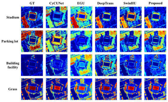
Figure 10.
Ground truth and extracted abundance maps for the Houston dataset using different HU methods (CyCU-Net, EGU, DeepTrans, SwinHU, and PICT-Net). The colors represent the abundance values from blue (sk = 0) to red (sk = 1).
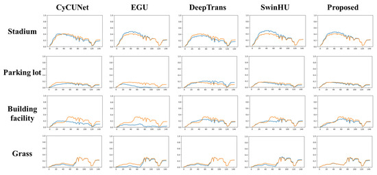
Figure 11.
Ground truth endmember spectra and extracted endmember spectra for the Houston dataset using different HU methods (CyCU-Net, EGU, DeepTrans, SwinHU, and PICT-Net). The yellow line is the ground truth, and the blue line represents the endmembers estimated by the HU methods.
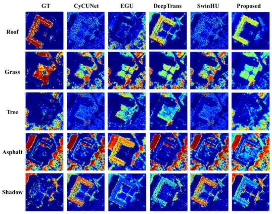
Figure 12.
Ground truth and extracted abundance maps for muffle dataset using different HU methods (CyCU-Net, EGU, DeepTrans, SwinHU, and PICT-Net). The colors represent the abundance values from blue (sk = 0) to red (sk = 1).
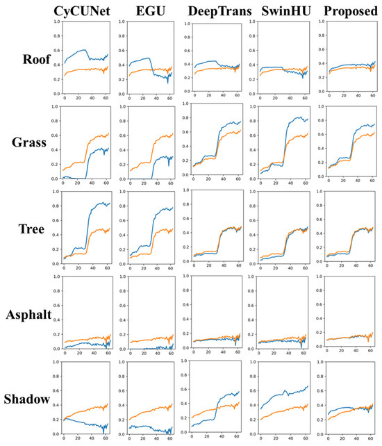
Figure 13.
Ground truth endmember spectra and extracted endmember spectra for the muffle dataset using different HU methods (CyCU-Net, EGU, DeepTrans, SwinHU, and PICT-Net). The yellow line is the ground truth, and the blue line represents the endmembers estimated by the HU methods.
From the above results, it can be seen that PICT-Net performs well across all the datasets and demonstrates advantages in terms of unmixing.
3.5. Ablation Study
To validate the effectiveness of different modules within the model, we removed or altered various model components and recorded changes in model performance, thereby demonstrating the contribution of each component. According to the main contributions of this paper, ablation experiments were conducted on the Transformer structure, hyperspectral feature extraction block, and prior knowledge. The specific details are as follows.
3.5.1. Transformer Structure
To examine the effectiveness of the Transformer architecture, we kept the other strategies used in our approach unchanged and replaced the main framework with a common encoder–decoder architecture, which is usually taken as the backbone in unmixing networks. The results are shown in Table 4.
Table 4.
Ablation study for comparing encoder–decoder architecture with the Transformer architecture on 4 datasets (Samosn, Apex, Houston and muffle). The best performances are shown in Bold.
It is evident from the experiments that the Transformer architecture performs better on all four datasets compared to the encoder–decoder architecture, thus proving the effectiveness of the Transformer architecture within this approach.
3.5.2. Hyperspectral Feature Extraction Block
The hyperspectral feature extraction block of most deep learning models uses a multi-layer convolutional encoder. In this model, the maximum pooling and average pooling operations are combined with a three-layer convolution. To test the effectiveness of the design of hyperspectral feature extraction blocks, the proposed hyperspectral feature extraction block and three-layer convolution operation are embedded into the model, respectively, for comparison.
According to multiple experiments, the best dimensionality reduction parameters were selected, and the bands out of the three-layer convolution are 128, 64, and 24, respectively. The experiment was performed on all four datasets and the results are shown in Table 5, which demonstrates that the proposed model is more beneficial for measuring the results of unmixing.
Table 5.
Ablation study for comparing traditional CNN feature extraction method with the proposed model on 4 datasets (Samosn, Apex, Houston and muffle). The best performances are shown in bold.
3.5.3. Prior Knowledge
- 1.
- Remove prior knowledge
This model extracts prior knowledge through the upper branch network; to check whether the prior knowledge extraction has a positive impact on the unmixing results, the upper branch of the model is removed to check the unmixing effect of the model. Under the condition of the consistent hyperparameter settings of the lower branch, an ablation experiment was conducted by removing the upper stream network to remove the incorporation of prior knowledge.
From the Figure 14, it can be observed that when no prior knowledge is included, the endmember fitting is not as good as when prior knowledge is added, and there is endmember variability for the endmember of water in the absence of the upper stream.
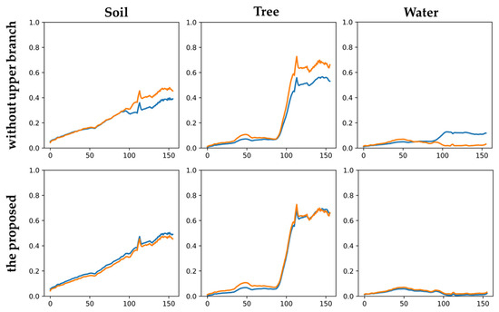
Figure 14.
Ablation study on prior knowledge obtained from upper branch. Ground truth endmember spectra and extracted endmember spectra of the Samson dataset without the upper branch model and PICT-Net. The yellow line is the ground truth, and the blue line represents the endmembers estimated by models.
More extensive experiments have been conducted, and the results indicate that, without incorporating prior knowledge, the model generates endmember variability more frequently than when using this method. This highlights the effectiveness of incorporating prior knowledge from the upper stream.
- 2.
- Modifying the quality of prior knowledge
Within a certain range, the larger the epoch of the upper branch, the higher the quality of the learned prior knowledge. By varying the epochs in the upper branch, the quality of the prior knowledge can be adjusted. The number of epochs in the upper branch network is changed to compare the unmixing results. The results are shown in Figure 15.
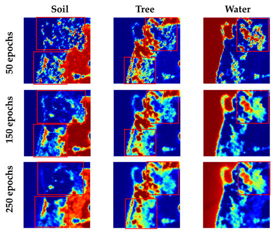
Figure 15.
Extracted abundance maps of the Samson dataset by changing the number of epochs in the upper branch. The colors represent the abundance values from blue (sk = 0) to red (sk = 1).
It can be found that, within a certain epoch range, a higher quality of prior knowledge results in more detailed information being learned from the abundance maps.
4. Conclusions
In this study, a dual-stream HSI unmixing model of data-coordinated optimization based on the Transformer architecture was proposed. This model uses a dual-stream network based on the Transformer architecture to reduce endmember variability during the hyperspectral unmixing process and enhance the model’s generalization ability and unmixing accuracy across different scenarios by using the weight-sharing strategy to extract prior knowledge. Experiments on four real datasets demonstrate the overall superiority of this method over other methods and the effectiveness of different components of the model was rigorously validated through ablation studies.
5. Discussion
Experimental results demonstrated that while enhancing the model’s global modeling capability, the approach ingeniously leverages data itself to refine the guidance for unmixing outcomes, thereby improving unmixing accuracy. However, this method focuses on enhancing unmixing precision at the expense of model speed; thus, future research will consider the computational complexity of the model to propose a more efficient unmixing model. Additionally, in subsequent work, we aim to investigate the relationship between unmixing results and the feedback mechanisms inherent to the model, with the objective of developing an unmixing model with superior generalization capabilities.
Author Contributions
Conceptualization, Y.Z. and J.Z.; methodology, Y.Z. and N.M.; software, N.M.; validation, Y.Z., J.Z. and W.L.; formal analysis, N.M.; investigation, W.L.; writing—original draft preparation, N.M.; writing—review and editing, Y.Z. and J.Z.; visualization, W.L.; supervision, Y.Z. and J.Z.; funding acquisition, Y.Z. and J.Z. All authors have read and agreed to the published version of the manuscript.
Funding
This research was funded by National Key Laboratory of Unmanned Aerial Vehicle Technology in NPU with grant number WR2024132, the National Natural Science Foundation of China with grant number 61801018, the Natural Science Basic Research Program of Shaanxi with grant number 2023-JC-QN-0769, and the Fundamental Research Funds for the Central Universities with grant number FRF-GF-20-13B.
Data Availability Statement
The data presented in this study are openly available in samson dataset apex dataset at [https://github.com/preetam22n/DeepTrans-HSU], and houston dataset muffle dataset at [https://github.com/hanzhu97702/IEEE_TGRS_MUNet/tree/main/data], reference number [10].
Conflicts of Interest
The authors declare no conflicts of interest.
References
- Liu, J.; Lan, J.; Zeng, Y. GL-Pooling: Global–Local Pooling for Hyperspectral Image Classification. IEEE Geosci. Remote Sens. Lett. 2023, 20, 5509305. [Google Scholar] [CrossRef]
- Hong, D.; Gao, L.; Yao, J.; Yokoya, N.; Chanussot, J.; Heiden, U.; Zhang, B. Endmember-Guided Unmixing Network (EGU-Net): A General Deep Learning Framework for Self-Supervised Hyperspectral Unmixing. IEEE Trans. Neural Netw. Learn. Syst. 2022, 33, 6518–6531. [Google Scholar] [CrossRef] [PubMed]
- Su, Y.; Li, J.; Plaza, A.; Marinoni, A.; Gamba, P.; Chakravortty, S. DAEN: Deep Autoencoder Networks for Hyperspectral Unmixing. IEEE Trans. Geosci. Remote Sens. 2019, 57, 4309–4321. [Google Scholar] [CrossRef]
- Ozkan, S.; Kaya, B.; Akar, G.B. EndNet: Sparse AutoEncoder Network for Endmember Extraction and Hyperspectral Unmixing. IEEE Trans. Geosci. Remote Sens. 2019, 57, 482–496. [Google Scholar] [CrossRef]
- Palsson, B.; Ulfarsson, M.O.; Sveinsson, J.R. Convolutional Autoencoder for Spectral–Spatial Hyperspectral Unmixing. IEEE Trans. Geosci. Remote Sens. 2021, 59, 535–549. [Google Scholar] [CrossRef]
- Wang, M.; Zhao, M.; Chen, J.; Rahardja, S. Nonlinear Unmixing of Hyperspectral Data via Deep Autoencoder Networks. IEEE Geosci. Remote Sens. Lett. 2019, 16, 1467–1471. [Google Scholar] [CrossRef]
- Gao, L.; Han, Z.; Hong, D.; Zhang, B.; Chanussot, J. CyCU-Net: Cycle-Consistency Unmixing Network by Learning Cascaded Autoencoders. IEEE Trans. Geosci. Remote Sens. 2022, 60, 5503914. [Google Scholar] [CrossRef]
- Deshpande, V.S.; Bhatt, J.S. A Practical Approach for Hyperspectral Unmixing Using Deep Learning. IEEE Geosci. Remote Sens. Lett. 2022, 19, 5511505. [Google Scholar] [CrossRef]
- Vaswani, A.; Shazeer, N.; Parmar, N.; Uszkoreit, J.; Jones, L.; Gomez, A.N.; Kaiser, L.; Polosukhin, I. Attention Is All You Need. arXiv 2017. [Google Scholar] [CrossRef]
- Ghosh, P.; Roy, S.K.; Koirala, B.; Rasti, B.; Scheunders, P. Hyperspectral Unmixing Using Transformer Network. IEEE Trans. Geosci. Remote Sens. 2022, 60, 5535116. [Google Scholar] [CrossRef]
- Duan, S.; Li, J.; Song, R.; Li, Y.; Du, Q. Unmixing-Guided Convolutional Transformer for Spectral Reconstruction. Remote Sens. 2023, 15, 2619. [Google Scholar] [CrossRef]
- Kong, F.; Zheng, Y.; Li, D.; Li, Y.; Chen, M. Window Transformer Convolutional Autoencoder for Hyperspectral Sparse Unmixing. IEEE Geosci. Remote Sens. Lett. 2023, 20, 5508305. [Google Scholar] [CrossRef]
- Duan, Y.; Xu, X.; Li, T.; Pan, B.; Shi, Z. UnDAT: Double-Aware Transformer for Hyperspectral Unmixing. IEEE Trans. Geosci. Remote Sens. 2023, 61, 5522012. [Google Scholar] [CrossRef]
- Yang, Z.; Xu, M.; Liu, S.; Sheng, H.; Wan, J. UST-Net: A U-Shaped Transformer Network Using Shifted Windows for Hyperspectral Unmixing. IEEE Trans. Geosci. Remote Sens. 2023, 61, 5528815. [Google Scholar] [CrossRef]
- Hadi, F.; Yang, J.; Farooque, G.; Xiao, L. Deep convolutional Transformer network for hyperspectral unmixing. Eur. J. Remote Sens. 2023, 56, 2268820. [Google Scholar] [CrossRef]
- Wang, Y.; Shi, S.; Chen, J. Efficient Blind Hyperspectral Unmixing with Non-Local Spatial Information Based on Swin Transformer. In Proceedings of the IGARSS 2023—2023 IEEE International Geoscience and Remote Sensing Symposium, Pasadena, CA, USA, 16–21 July 2023; pp. 5898–5901. [Google Scholar]
- Wang, L.; Zhang, X.; Zhang, J.; Dong, H.; Meng, H.; Jiao, L. Pixel-to-Abundance Translation: Conditional Generative Adversarial Networks Based on Patch Transformer for Hyperspectral Unmixing. IEEE J. Sel. Top. Appl. Earth Obs. Remote Sens. 2024, 17, 5734–5749. [Google Scholar] [CrossRef]
- Bhakthan, S.M.; Loganathan, A. A hyperspectral unmixing model using convolutional vision transformer. Earth Sci. Inf. 2024, 17, 2255–2273. [Google Scholar] [CrossRef]
- Chen, J.; Yang, C.; Zhang, L.; Yang, L.; Bian, L.; Luo, Z.; Wang, J. TCCU-Net: Transformer and CNN Collaborative Unmixing Network for Hyperspectral Image. IEEE J. Sel. Top. Appl. Earth Obs. Remote Sens. 2024, 17, 8073–8089. [Google Scholar] [CrossRef]
- Xu, C.; Ye, F.; Kong, F.; Li, Y.; Lv, Z. MSCC-ViT: A Multiscale Visual-Transformer Network Using Convolution Crossing Attention for Hyperspectral Unmixing. IEEE J. Sel. Top. Appl. Earth Obs. Remote Sens. 2024, 17, 18070–18082. [Google Scholar] [CrossRef]
- Yang, Y.; Wang, Y.; Liu, T. CDCTA: Cascaded dual-constrained transformer autoencoder for hyperspectral unmixing with endmember variability and spectral geometry. J. Appl. Remote Sens. 2024, 18, 026502. [Google Scholar] [CrossRef]
- Ge, Y.; Han, L.; Paoletti, M.E.; Haut, J.M.; Qu, G. Transformer-Enhanced CNN Based on Intensive Feature for Hyperspectral Unmixing. IEEE Geosci. Remote Sens. Lett. 2024, 21, 5510605. [Google Scholar] [CrossRef]
- Wang, P.; Liu, R.; Zhang, L. MAT-Net: Multiscale Aggregation Transformer Network for Hyperspectral Unmixing. IEEE Trans. Geosci. Remote Sens. 2024, 62, 5538115. [Google Scholar] [CrossRef]
- Li, Y.; Jiang, B.; Li, X.; Tian, J.; Song, X. Unsupervised hyperspectral unmixing based on robust nonnegative dictionary learning. J. Syst. Eng. Electron. 2022, 33, 294–304. [Google Scholar] [CrossRef]
- Meng, F.; Sun, H.; Li, J.; Xu, T. CTNet: An efficient coupled transformer network for robust hyperspectral unmixing. Int. J. Remote Sens. 2024, 45, 5679–5712. [Google Scholar] [CrossRef]
- Wang, W.; Qian, Y.; Liu, H. Multiple Clustering Guided Nonnegative Matrix Factorization for Hyperspectral Unmixing. IEEE J. Sel. Top. Appl. Earth Obs. Remote Sens. 2020, 13, 5162–5179. [Google Scholar] [CrossRef]
- Li, E.; Zhu, S.; Zhou, X.; Yu, W. The development and comparison of endmember extraction algorithms using hyperspectral imagery. J. Remote Sens. 2011, 15, 659–679. [Google Scholar] [CrossRef]
- Rasti, B.; Hong, D.; Hang, R.; Ghamisi, P.; Kang, X.; Chanussot, J.; Benediktsson, J.A. Feature Extraction for Hyperspectral Imagery: The Evolution From Shallow to Deep: Overview and Toolbox. IEEE Geosci. Remote Sens. Mag. 2020, 8, 60–88. [Google Scholar] [CrossRef]
Disclaimer/Publisher’s Note: The statements, opinions and data contained in all publications are solely those of the individual author(s) and contributor(s) and not of MDPI and/or the editor(s). MDPI and/or the editor(s) disclaim responsibility for any injury to people or property resulting from any ideas, methods, instructions or products referred to in the content. |
© 2025 by the authors. Licensee MDPI, Basel, Switzerland. This article is an open access article distributed under the terms and conditions of the Creative Commons Attribution (CC BY) license (https://creativecommons.org/licenses/by/4.0/).