Article

Quantifying Tree Structural Change in an African Savanna by Utilizing Multi-Temporal TLS Data

1
Department for Earth Observation, Friedrich Schiller University Jena, Löbdergraben 32, 07743 Jena, Germany
2
Department of Physical Geography, Friedrich Schiller University Jena, Löbdergraben 32, 07743 Jena, Germany
3
Unit of Computing Sciences, Tampere University, Korkeakoulunkatu 1, 33720 Tampere, Finland
4
Scientific Services, Savanna and Grassland Research Unit, South African National Parks (SANParks), Skukuza 1350, South Africa
5
School of Natural Resource Management, Nelson Mandela University, George Campus, George 6530, South Africa
6
Department of Organismic and Evolutionary Biology, Harvard University, Cambridge, MA 02138, USA
*
Author to whom correspondence should be addressed.
Remote Sens. 2025, 17(5), 757; https://doi.org/10.3390/rs17050757
Submission received: 12 December 2024 / Revised: 21 January 2025 / Accepted: 17 February 2025 / Published: 22 February 2025
(This article belongs to the Special Issue Remote Sensing of Savannas and Woodlands II)

Abstract

:
Structural changes in savanna trees vary spatially and temporally because of both biotic and abiotic drivers, as well as the complex interactions between them. Given this complexity, it is essential to monitor and quantify woody structural changes in savannas efficiently. We implemented a non-destructive approach based on Terrestrial Laser Scanning (TLS) and Quantitative Structure Models (QSMs) that offers the unique advantage of investigating changes in complex tree parameters, such as volume and branch length parameters that have not been previously reported for savanna trees. Leaf-off multi-scan TLS point clouds were acquired during the dry season, using a Riegl VZ1000 TLS, in September 2015 and October 2019 at the Skukuza flux tower in Kruger National Park, South Africa. These three-dimensional (3D) data covered an area of 15.2 ha with an average point density of 4270 points/m2 (0.015°) and 1600 points/m2 (0.025°) for the 2015 and 2019 clouds, respectively. Individual tree segmentation was applied on the two clouds using the comparative shortest-path algorithm in LiDAR 360(v5.4) software. We reconstructed optimized QSMs and assessed tree structural parameters such as Diameter at Breast Height (DBH), tree height, crown area, volume, and branch length at individual tree level. The DBH, tree height, crown area, and trunk volume showed significant positive correlations (R2 > 0.80) between scanning periods regardless of the difference in the number of points of the matched trees. The opposite was observed for total and branch volume, total number of branches, and 1st-order branch length. As the difference in the point densities increased, the difference in the computed parameters also increased (R2 < 0.63) for a high relative difference. A total of 45% of the trees present in 2015 were identified in 2019 as damaged/felled (75 trees), and the volume lost was estimated to be 83.4 m3. The results of our study showed that volume reconstruction algorithms such as TreeQSMs and high-resolution TLS datasets can be used successfully to quantify changes in the structure of savanna trees. The results of this study are key in understanding savanna ecology given its complex and dynamic nature and accurately quantifying the gains and losses that could arise from fire, drought, herbivory, and other abiotic and biotic disturbances.

1. Introduction

Savanna ecosystems cover 50% of terrestrial territory in Africa and play a crucial role in the global carbon cycle [1]. These ecosystems consist of a mix of woody vegetation and grasses in varying ratios, which change spatially and temporally, ranging from minimal woody cover to dense thickets with over 80% coverage [2,3]. The spatial variation in woody cover is essential for savanna ecosystems’ maintenance and proper functionality [3]. However, savannas are highly dynamic systems, and vegetation structure constantly changes due to the interaction of various drivers, including human interference, herbivory, fire and drought [4,5]. These factors can lead to broad-scale directional shifts in woody vegetation.
Information on changes in vegetation structure is crucial for park management, as these alterations have cascading effects on other ecosystem patterns, processes [6] and fauna [3]. Accurately quantifying these dynamics in savanna ecosystems is essential for understanding ecological processes and ecosystem functioning [7]. Spatiotemporal information is necessary to comprehend the interaction of these drivers across varying temporal and spatial scales [8]. Terrestrial Laser Scanning (TLS) provides the capability to detect spatiotemporal changes.
In recent years, TLS has gained significant interest as an alternative method for accurately quantifying tree structure at individual and plot scales [9,10,11]. In open savannas, where trees are sparsely distributed at densities of 10–40 trees/ha, TLS proves to be an efficient tool for characterizing vegetation structure. With precise data collection techniques and models for tree structure, such as Quantitative Structure Models (QSMs) [12], the reconstructed tree models are geometrically accurate and can be utilized to derive various attributes of interest [8,10].
The non-destructive nature of TLS enables the collection of subsequent measurements, facilitating multi-temporal analyses of the growth and evolution of forest stands over time [13]. It also allows for the quantification of small-scale changes in tree attributes and canopy structure [14]. Multi-temporal studies have been successfully conducted to quantify changes in Above Ground Biomass (AGB) and assess structural changes across various ecosystems. Bogdanovich et al. (2021) [7] used multi-temporal TLS to evaluate the impact of tree management on tree structural properties and growth in a Mediterranean open woodland, and they reported that crown area increased more than height and that pruned trees showed larger changes in crown area compared to the controlled trees. Srinivasan et al. (2014) [15] also used multi-temporal TLS to estimate tree-level AGB change in East Texas, and they concluded that direct modelling of AGB change with TLS data provided the best results for loblolly pines compared with modelling with field and TLS data. Yrttimaa et al. (2020) [8] assessed the accuracy and feasibility of TLS in quantifying change in the structure of boreal forests, and they confirmed the capacity of TLS to quantify change in tree and forest structural attributes with an increase or a decrease in tree and forest attributes recorded in the field that gave a similar outcome with bi-temporal TLS data. Kaasalainen et al. (2014) [16] & Sheppard et al. (2017) [10] both used multi-temporal TLS data and QSMs to quantify the change in biomass and assess tree growth, respectively. The loss of major branches could be detected, and changes in tree branching structure could be reproduced with ± 10% accuracy [16]. The availability of QSMs based on TLS data allowed the accurate determination of crown attributes as well as volume as a result of tree pruning [10]. Changes in forest structure over time were achieved with bi-temporal TLS, and they observed that TLS data collected at different times to detect tree stem changes can be fully automated [13].
Although structural changes in savanna vegetation have been studied using airborne light detection and ranging (Lidar) [4], TLS offers super precision and resolution compared with airborne lidar [7]. Given the dynamic nature of savanna ecosystems, our understanding of monitoring savanna vegetation structure using multi-temporal TLS datasets and QSMs remains limited. This study builds upon previous research by integrating high-resolution data from the TLS with the capability of the QSMs to provide accurate geometric models that hierarchically describe trees, allowing for the extraction of various tree attributes [17,18]. Furthermore, we utilize QSMs to investigate changes in complex tree parameters, such as trunk volume, total volume and branch volume, and both total and 1st-order branch lengths, parameters that have not been previously reported for savanna trees. We establish the reliability and potential biases of our method in quantifying tree structural changes following an event and provide recommendations for future research. Additionally, we identify the interacting drivers that influence vegetation structure by quantifying felled and damaged trees, as well as the total volume lost. Moreover, we quantify subtle changes in the tree structure without relying on field surveys, which may lack accuracy. This study holds significant ecological importance, particularly for assessing vegetation structure to facilitate effective park management.
This study aimed at quantifying tree structural changes in a savanna ecosystem following disturbances, utilizing multi-temporal TLS data collected over four years, specifically between September 2015 and October 2019. The primary disturbances included the droughts of 2015 and 2016, which were exacerbated by an El Niño event [19], as well as herbivory by elephants, which tends to increase during drought conditions [20]. However, other contributing factors such as fire [21], climate change [22], human activity [23], soil properties [24] and biological invasions [25] were not ruled out. We assessed changes in DBH (diameter at breast height), tree height, crown area, volume, and branch length at the individual tree level and evaluated the impact of these interacting drivers on tree growth and structure. The main objectives of the study are as follows:
  • To quantify the change in tree structure by analyzing the change in (DBH, height and crown area, volume, and branch length) in the four years
  • Discuss the factors driving changes in tree structure, specifically focusing on elephants and drought
The manuscript is organized as follows: Section 2 outlines the methods, while Section 3 details the main results of the study. Section 4 and Section 5 present the discussion points and conclusions derived from the research.

2. Materials and Methods

2.1. Study Site

This study was conducted in Kruger National Park, South Africa (23°98′S, 31°55′E), around the Skukuza eddy covariance (EC) flux tower, encompassing a total area of 55 hectares. The analysis focused on a 15.2-hectare section designated as a matched tree area (Figure 1), as it was more centrally located relative to the scanning positions from both scanning periods. The landscape at the site is relatively flat, situated at an altitude of 365 m above sea level (a.s.l). It is dominated by species such as Combretum, Sclerocarya, Vachellia, and Senegalia species, which range in height from two to ten meters [26,27]. The soils are characterized as nutrient-poor, sandy textures derived from granite [28]. The region is semi-arid, with rainfall occurring from late October to February. Although the long-term average annual rainfall is 550 mm/yr [28], the period between the scanning dates experienced a drought. The structure and functionality of the savanna are influenced by water availability [29,30], and prolonged periods of insufficient rainfall combined with high temperatures have been shown to increase tree mortality [29,31]. However, tree species vary in their capability to withstand and recover from the effects of droughts [32,33].

2.2. Terrestrial Laser Scanning and Data Pre-Processing

We mapped the study area with a multiple-return Terrestrial LiDAR Scanner (TLS) in September 2015 and October 2019 with a Riegl VZ 1000 laser scanner [34] (RIEGL Laser Measurement Systems GmbH, Horn, Austria). The TLS was mounted on termite mounds, and data were collected at a height of 2 m above ground level, employing an angular sampling of 0.015° for 2015 and 0.025° for 2019 with a pulse repetition rate of 300 kHz. TLS scans were obtained from 30 scan positions in September 2015 and 32 scan positions in October 2019, arranged in a circular pattern around the flux tower, utilizing a total of 81 tie points for precise geo-referencing of the scans based on a differential Global Navigation Satellite System (dGNSS) linked to the South African Trignet of permanently receiving stations. The overall co-registration accuracy was 0.03 m. The scan settings used during the two scanning periods are summarised in Table 1 below.

2.3. Tree-to-Tree Matching

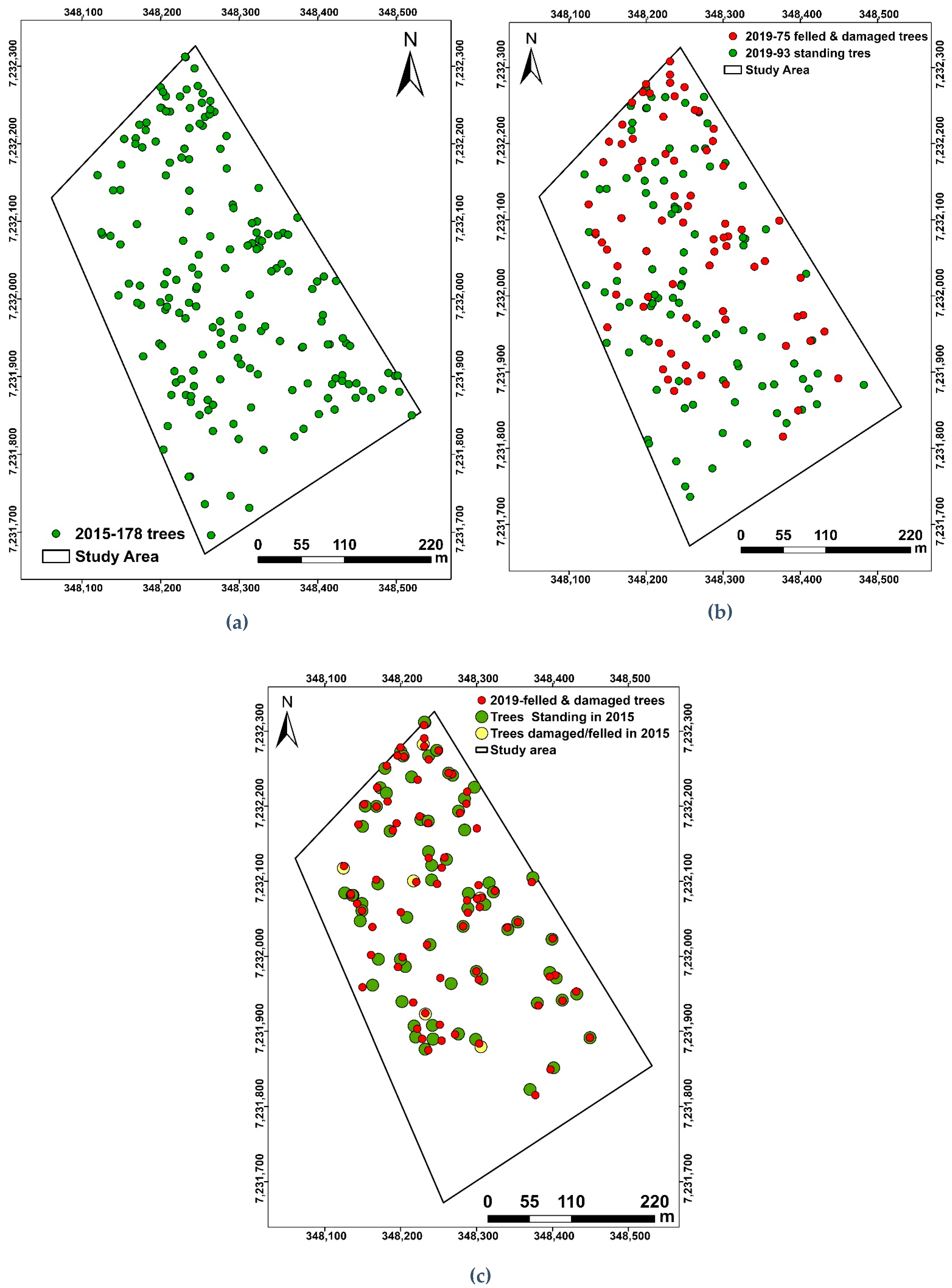
The point clouds from both years were processed in the same manner; point clouds were exported to Lidar 360 (v 5.4) software (Green Valley International © 2022, Berkeley, CA, USA) for individual tree segmentation. Since the segmentation is automated, the resulting segments were manually edited to correct any instances of under- or over-segmentation [35]. This editing resulted in 178 and 168 correctly segmented trees from 2015 and 2019, respectively (93 standing and 75 felled/damaged) (Figure 2a,b). A tree was considered correctly segmented when it was accurately distinguished and isolated from its surroundings, with a clearly defined trunk and crown structure, without any missing areas or gaps in the major parts of the tree [36]. In 2019, 75 trees were identified as damaged or felled, and the lost volume was computed. We also matched the seventy-five felled trees in 2019 to standing trees in 2015; sixty-nine trees were identified as standing in 2015 (marked in green in Figure 2c), while six trees were identified as damaged/felled in 2015 (marked in yellow in Figure 2c).
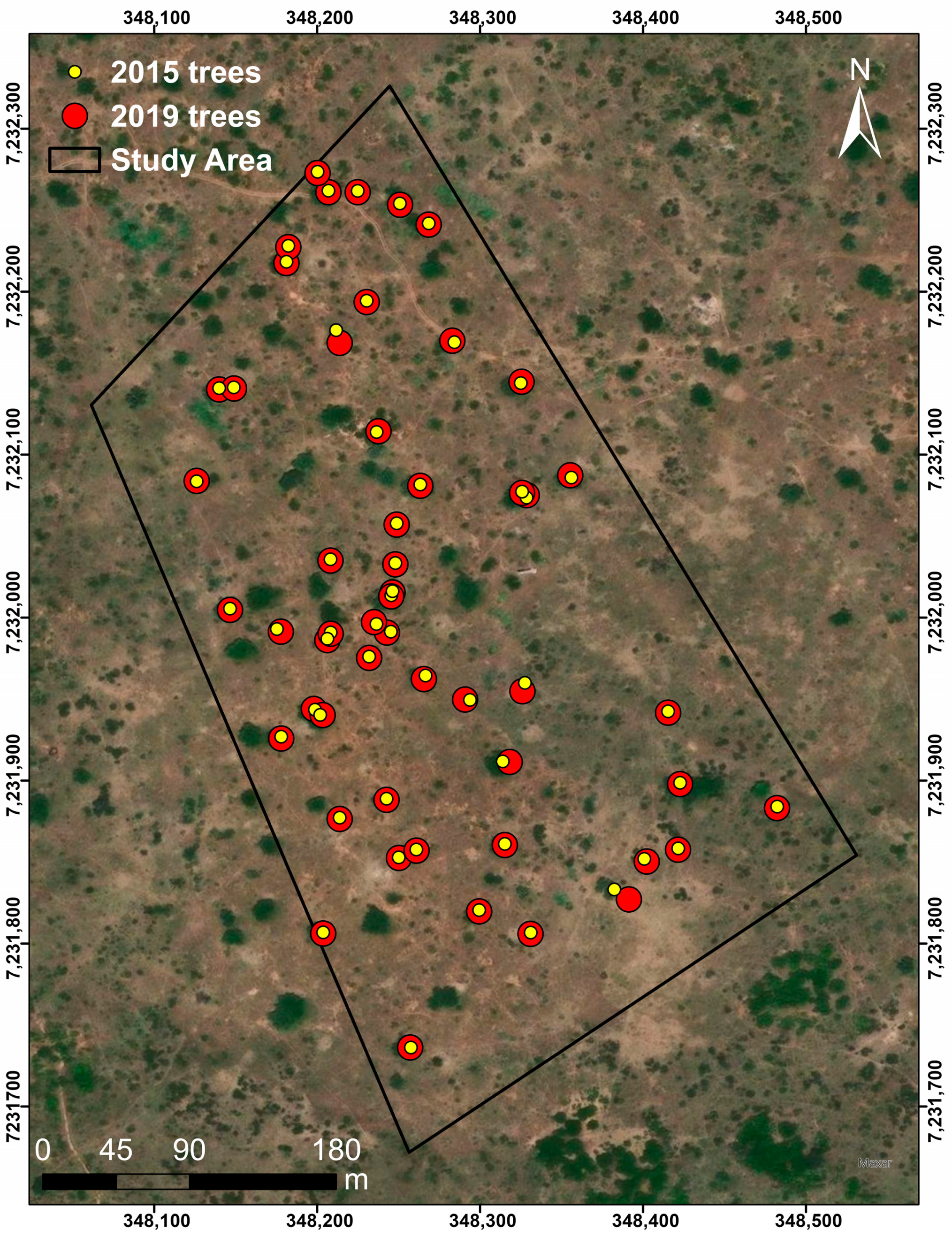
By overlaying segmented trees from 2019 on trees from 2015, a total of 53 trees were matched. Figure 3 below shows the location of the matched trees in the study area.
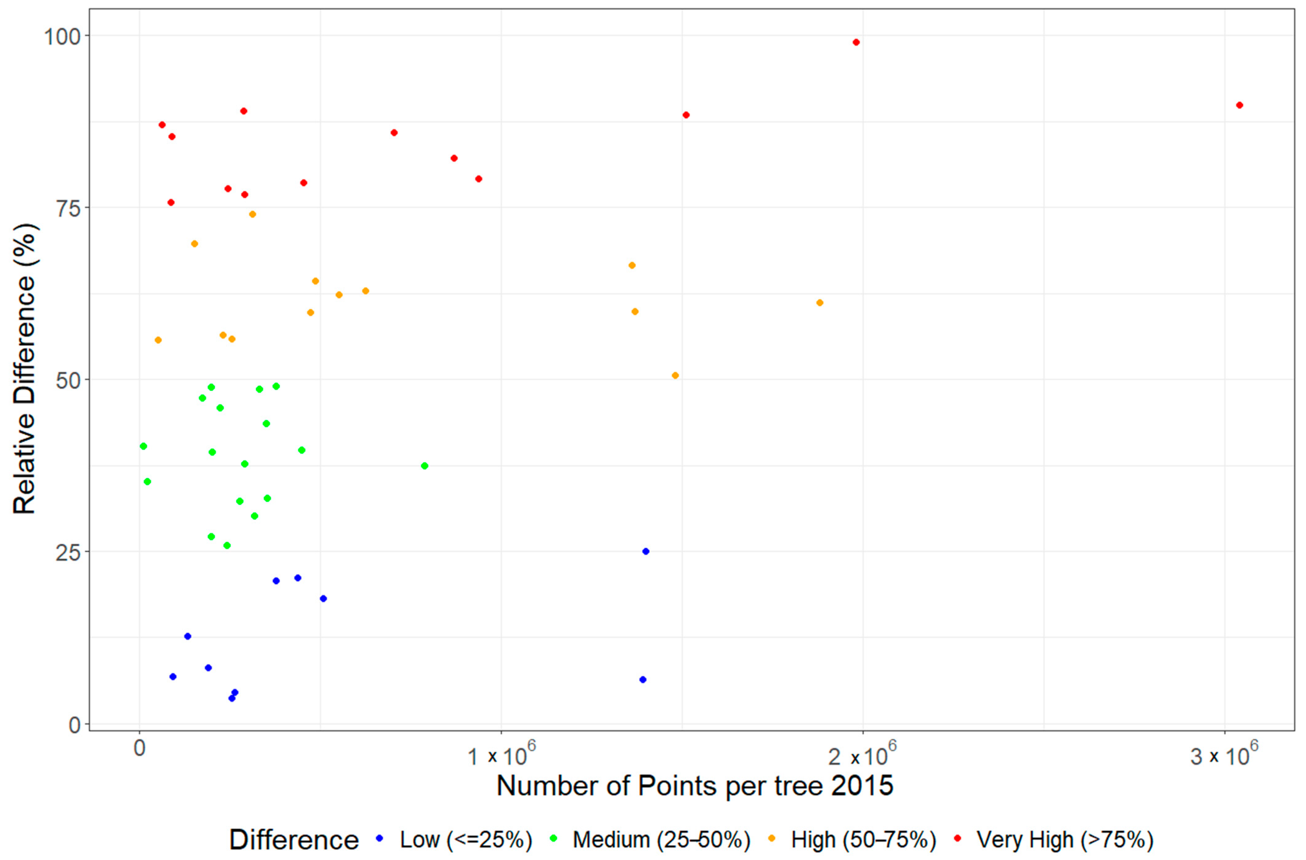
To account for the uncertainties associated with the differences in data acquisition methodologies between the 2015 and 2019 periods, specifically regarding variations in scan positions and scan resolutions, we computed the relative difference in the number of points per tree between the matched trees (Figure 4). Of the 53 trees, 13 had a very high (>75%), 13 had a high (50–75%), 17 had a medium (25–50%), and 10 had a low (≤25%) relative difference in number of points between 2015 and 2019. The relative difference was computed as follows (Equation (1)):
R e l a t i v e   d i f f e r e n c e = | # 2015 # 2019 | max ( # 2015 , # 2019 )
where #2015 denotes the number of points for the tree in the 2015 scan.
#2019 denotes the number of points for the tree in the 2019 scan.
Figure 4. Difference of points per tree between the matched trees. Very high (>75%), high (50–75%), Medium (25–50%), and Low (≤25%) relative difference.
Remotesensing 17 00757 g004
To derive the tree structural parameters (DBH, height, crown area, volume, and branch length) between the two scanning years, we employed Quantitative Structural Models (QSMs) reconstructed with TreeQSM (v2.4.0) developed by Raumonen et al. (2013, 2015) [12,37] and implemented in MATLAB (v 2022a). For each tree, we optimised the required input parameters of TreeQSM, and we generated 10 QSMs per tree with the optimal inputs because of the inherent randomness in the reconstruction process. The final estimated values for the tree structural parameters are the averages of these 10 QSMs, while the standard deviation provides an estimate of the uncertainty in the parameters. Table 2 below presents all the measured parameters. Changes in tree structural attributes were quantified by comparing the TLS-derived parameters from 2015 with those from 2019.

2.4. Statistical Analysis and Change Analysis

All statistical analyses were conducted using RStudio (R 4.2.2) (R Development Core Team, 2024) [38]. We analyzed the relationship between the parameters derived from the two scanning periods by employing least-square regression, focusing on the relative difference in the number of points per tree between the two scanning periods. The accuracy of the parameters derived in 2015 and 2019 was assessed by using the Coefficient of determination R2 (Equation (2)) and Root Mean Square Error (RMSE) to the 1:1 line (Equation (3)).
R 2 = 1 i = 1 n y i y ^ i 2 i = 1 n ( y i y ¯ )  
where n is the number of trees (=53), and
yi and ŷi are the measured values of the parameter for the tree i in 2015 and 2019, and y ¯ is the mean value in 2019.
R M S E =   1 n   i = 1 n y i y ^ i 2  
where n is the number of trees (=53), and
yi and ŷi are the measured values of the parameter for tree i in 2015 and 2019.
To compare the changes in each parameter, we divided the trees into diameter classes (<30 cm, 30–40 cm, 40–50 cm, 50–60 cm, and >60 cm) based on the DBH range of the matched trees from 2015. To assess whether there were any significant changes in the means of the parameters for each dbh class, we employed a t-test at a 95% level of significance. To determine which t-test to use, we conducted an F-test for two samples to compare variances.
The computation of Canopy Height Models (CHMs) was performed in Lidar 360 (v5.4). To eliminate the height discrepancies caused by elevation, the point clouds were first normalised by using classified ground points. The normalised clouds were used to generate the Digital Surface Models (DSM) and Digital Elevation Models (DEM) with a grid size of 1 m × 1 m based on the minimal resolution of the point cloud. The CHMs for both years were derived by subtracting the DEM from the DSM. The elevation difference between the CHMs was computed using a raster calculator in ArcMap (v 10.8.2).
To ground truth, the TLS measured DBH, and field measurements of DBH of the 53 matched trees were taken in September 2024. Of these 53 matched trees, 38 were identified in the field, as some were either dead or missing by the time of the survey. The DBH measured in the field was compared with the DBH estimated using the QSMs for the two scanning periods. A linear regression analysis was conducted to compare the TLS-derived DBH with the field-measured DBH. Of the matched trees, the species identified were Sclerocarya birrea, Senegalia nigrescens, Cassia abbreviata, and Peltophorum africanum, with Sclerocarya birrea being the most frequently encountered species (83%). This prevalence is attributed to the greater drought tolerance of Sclerocarya birrea to the other species [39,40].

3. Results

3.1. Canopy Height Models

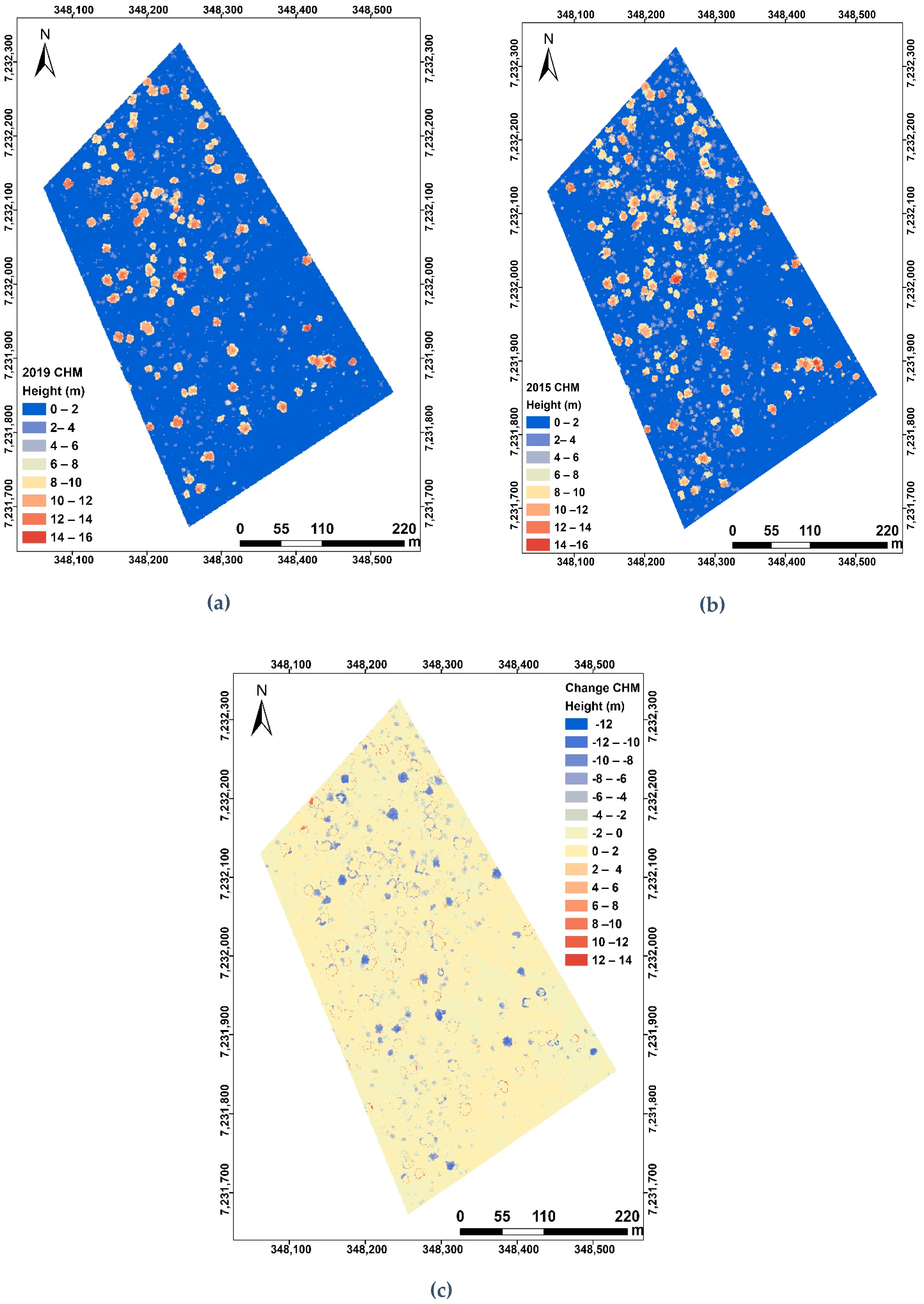
The elevation differences between the 2015 and 2019 canopy height models (CHMs) were computed (Figure 5a–c). A total of 45% of the trees present in 2015 were damaged or felled in 2019. The majority of the trees with a height of 4–12 m were lost between the 2015 and 2019 period, though some tall trees survived the drought and or herbivory as observed in the 4–14 m height range in the change CHM. The volume of the 75 trees that were identified as damaged or felled in 2019 was estimated through their QSMs. Of the seventy-five trees, eight failed to reconstruct acceptably; thus, the total lost volume (without those eight trees) was estimated to be 83 361 litres (83.4 m3).

3.2. Parameters Derived from the Two Scanning Periods

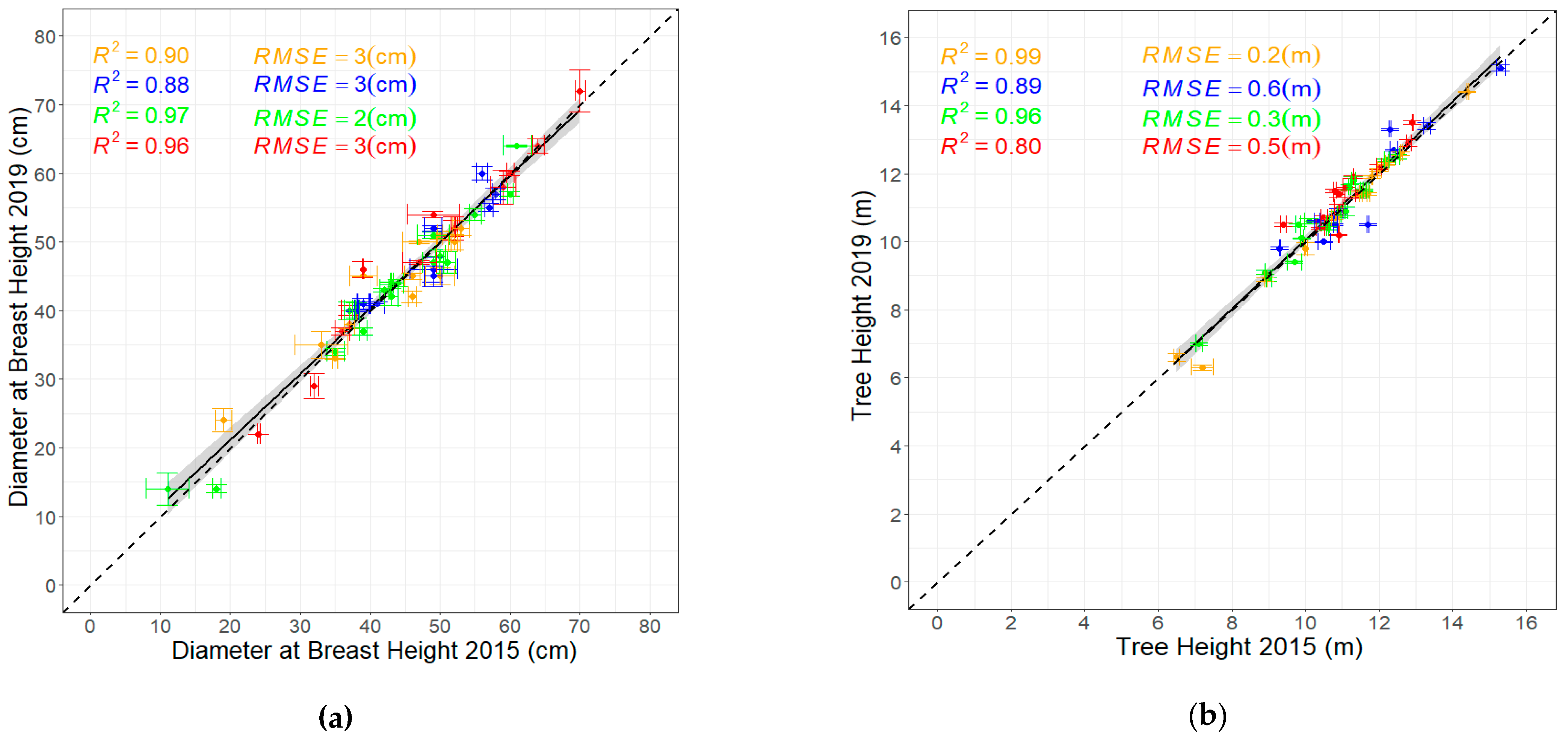
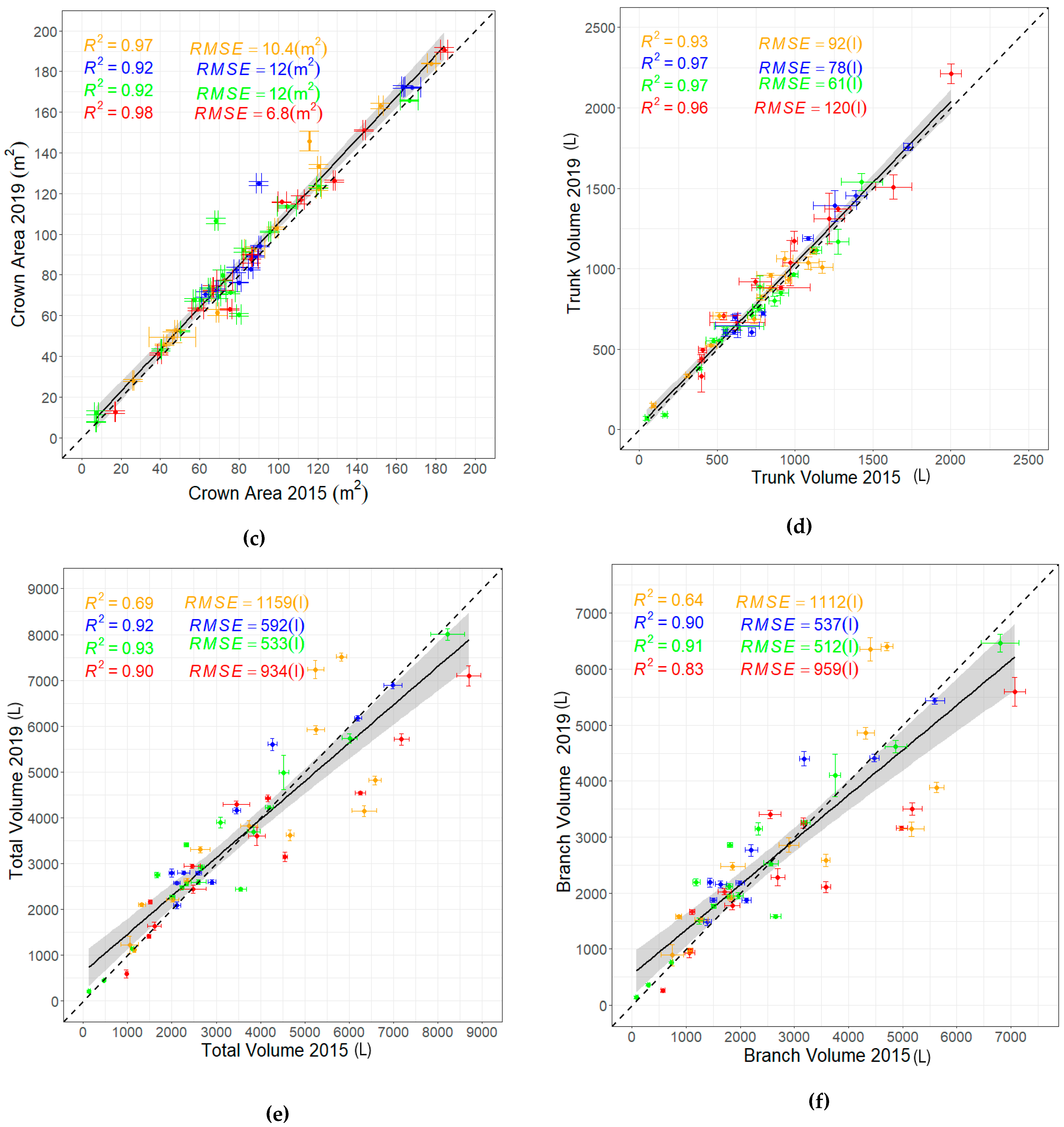
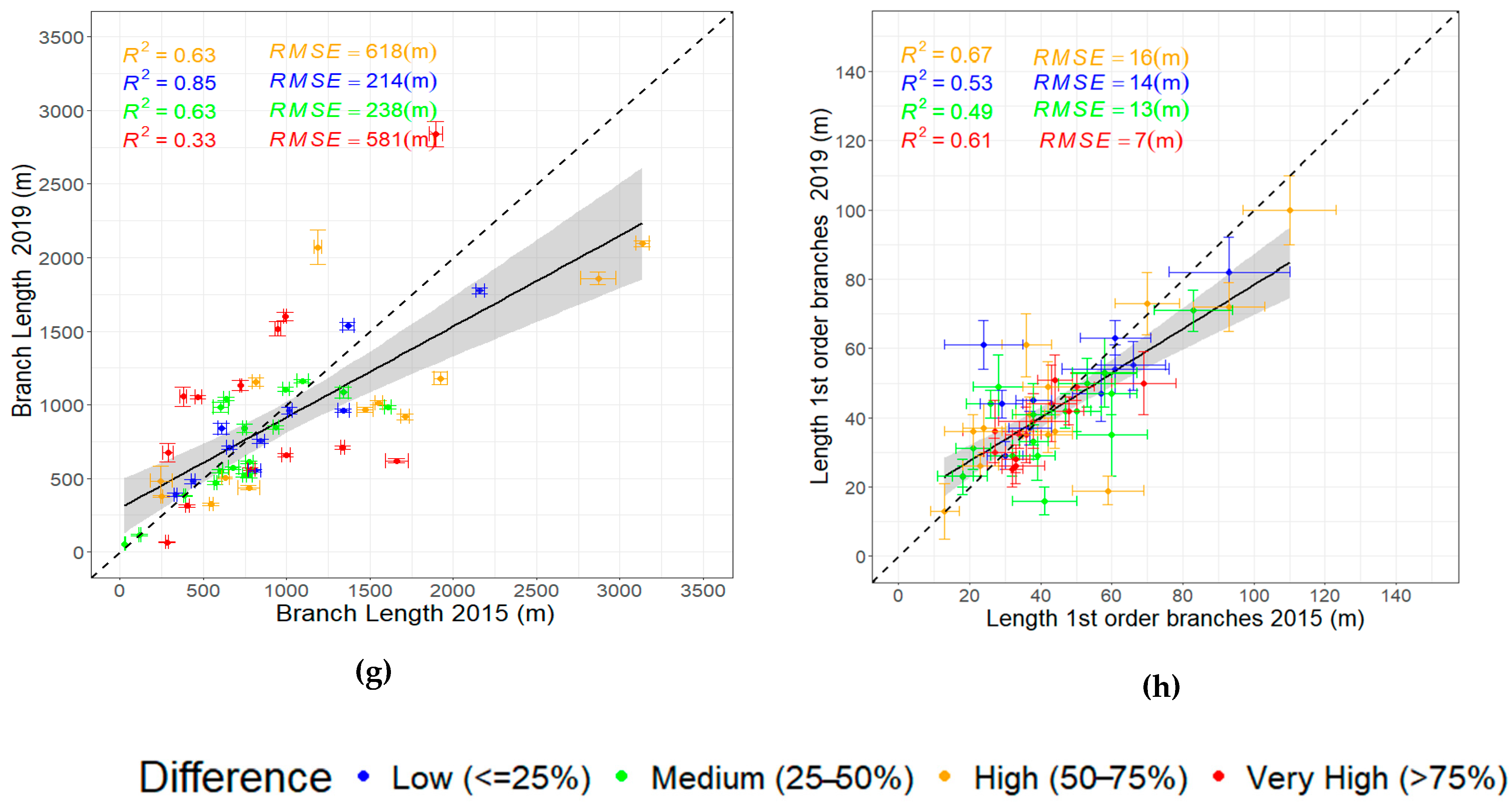
The change in tree structure between the two scanning periods was analysed by the change in DBH (Figure 6a), height (Figure 6b), crown area (Figure 6c), trunk volume (Figure 6d), total volume (Figure 6e), branch volume (Figure 6f), total branch length (Figure 6g), and branch length of first-order branches (Figure 6h), between the 53 matched trees. The DBH, tree height, crown area and trunk volume showed significant positive correlations (R2 > 0.80) between the two years of scanning regardless of the difference in the number of points of the matched trees (Figure 6a–d). The opposite was observed for the more complex tree parameters of total volume, branch volume, and branch length (Figure 6e–g). As the difference in the point densities increased, the difference in the computed parameters increased, as observed by the low correlation values for total volume (R2 = 0.69), 0.64 for branch volume and 0.63 for branch length for matched trees with a high relative difference (50–75%). The correlation is even lower (R2 = 0.33) for branch length for trees that have a very high (>75%) relative difference. For the 1st-order branch length Figure 6h, the lowest correlation (R2 = 0.49) was observed between matched trees with a medium relative difference (25–50%). The standard deviation of the computed length of the 1st-order branches between the two scanning periods is also relatively high.

3.3. Evaluating the Relationships Among Derived Tree Parameters

To evaluate the relationships among the derived tree structural parameters for each scanning period, we conducted an analysis calculating the correlation coefficient (R2) and the Residual Mean square Error (RMSE) for each possible combination and the results are shown in Table 3 below. DBH had a positive relationship with the majority of the tree parameters, with the most positive relationship observed for trunk volume (R2 = 0.91 and RMSE = 883 L and (R2 = 0.91 and RMSE = 913 L) for the years 2015 and 2019, respectively. The large errors for DBH were detected for tree parameters of tree height, branch and 1st-order branch length for both years. Tree height relationship with other parameters was relatively negative, with the largest RMSE reported for 1st-order branch length (RMSE = 38.3 m) for 2015 and with total branch length (RMSE = 822.3 m) for 2019. The large RMSEs reported with tree height could be attributed to the heterogeneity of the matched trees. For the parameter crown area, positive relationships were observed especially for volume parameters for both 2015 and 2019, respectively (Total volume R2 = 0.81, RMSE = 3656 L and R2 = 0.84, RMSE = 3756 L), (Branch volume R2 = 0.79, RMSE = 2765 L and R2 = 0.81, RMSE = 2825 L) and (Trunk volume R2 = 0.75, RMSE =863 L and R2 = 0.77, RMSE = 897 L). Confirming that crown area is a good predictor of tree volume. The best relationship among all the parameters was observed between total and branch volume (R2 = 0.99 and RMSE = 3066 L) and (R2 = 0.98 and RMSE = 3010 L) for the years 2015 and 2019, respectively. Generally, the most positive relationships were observed with the volume parameters and the weakest relationships with branch length parameters.

3.4. Comparing the Change in Tree Structural Parameters per Diameter Class

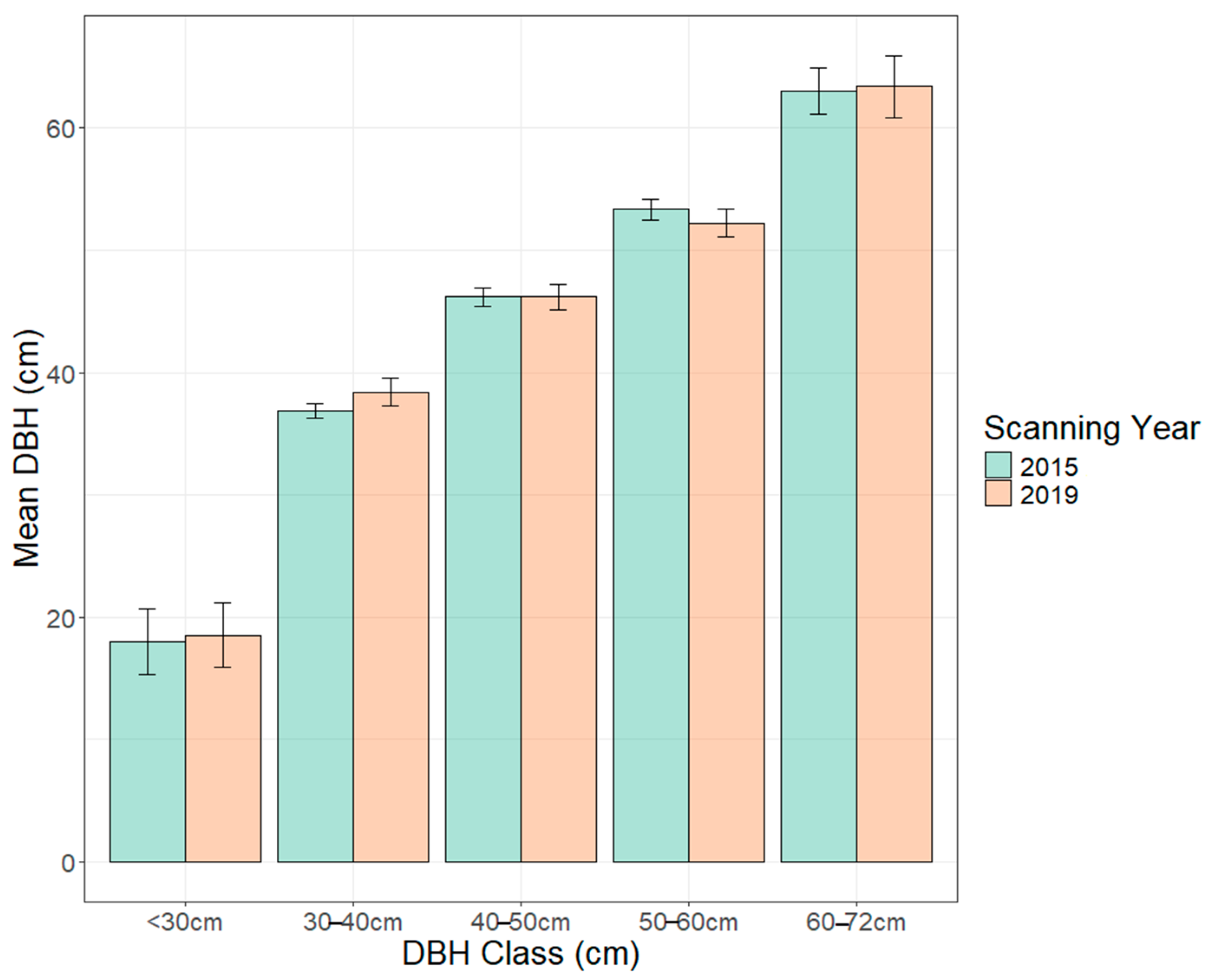
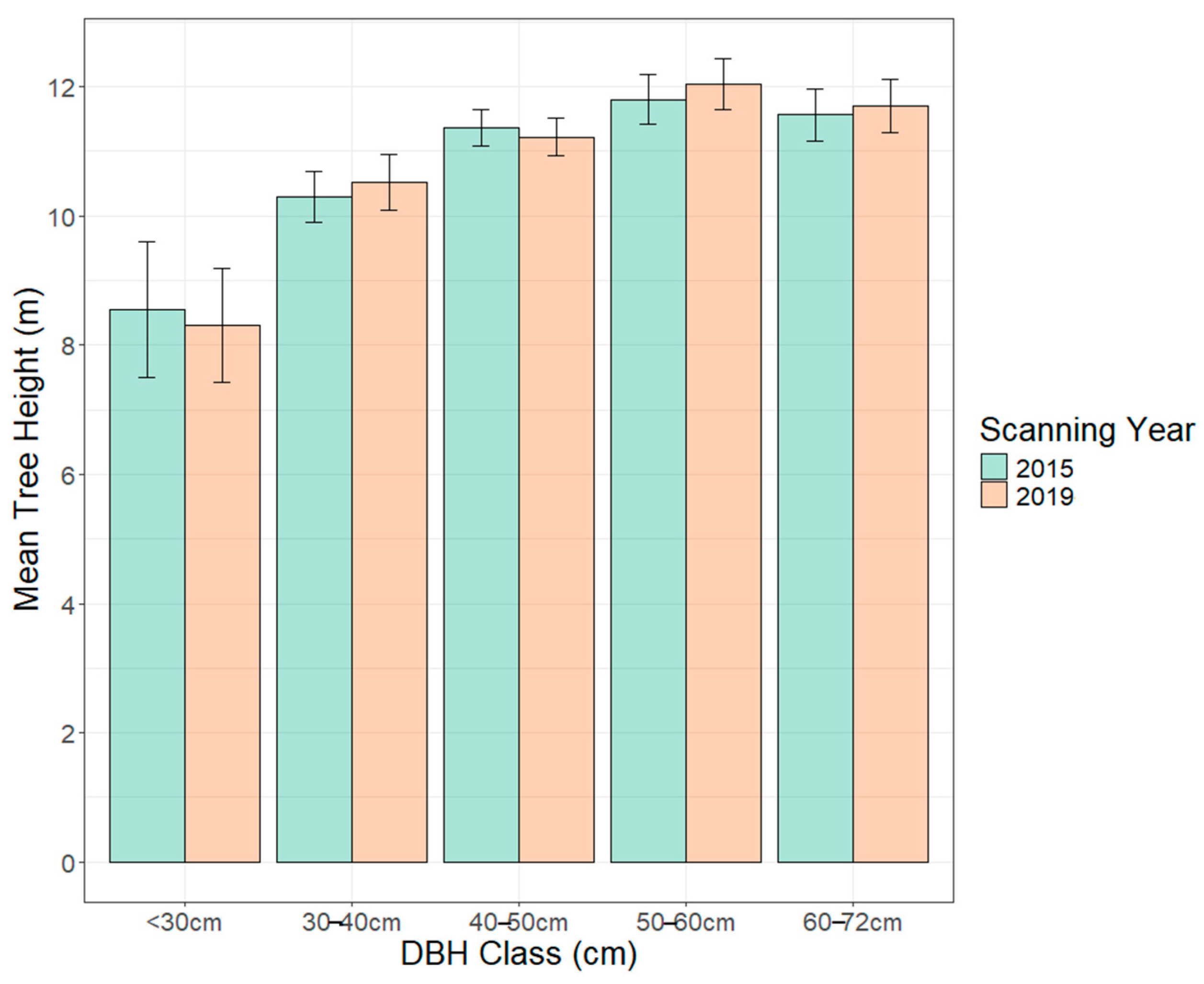
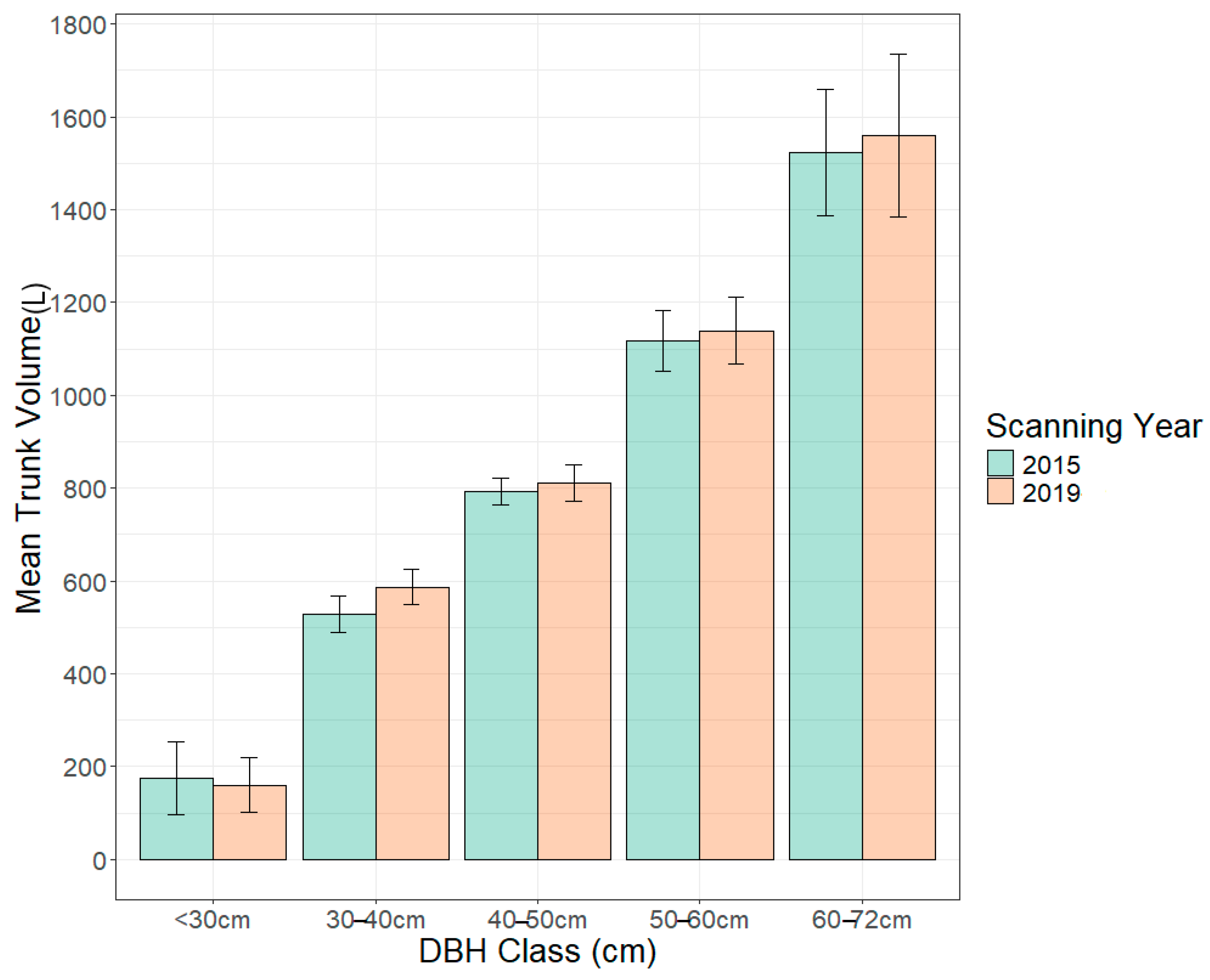
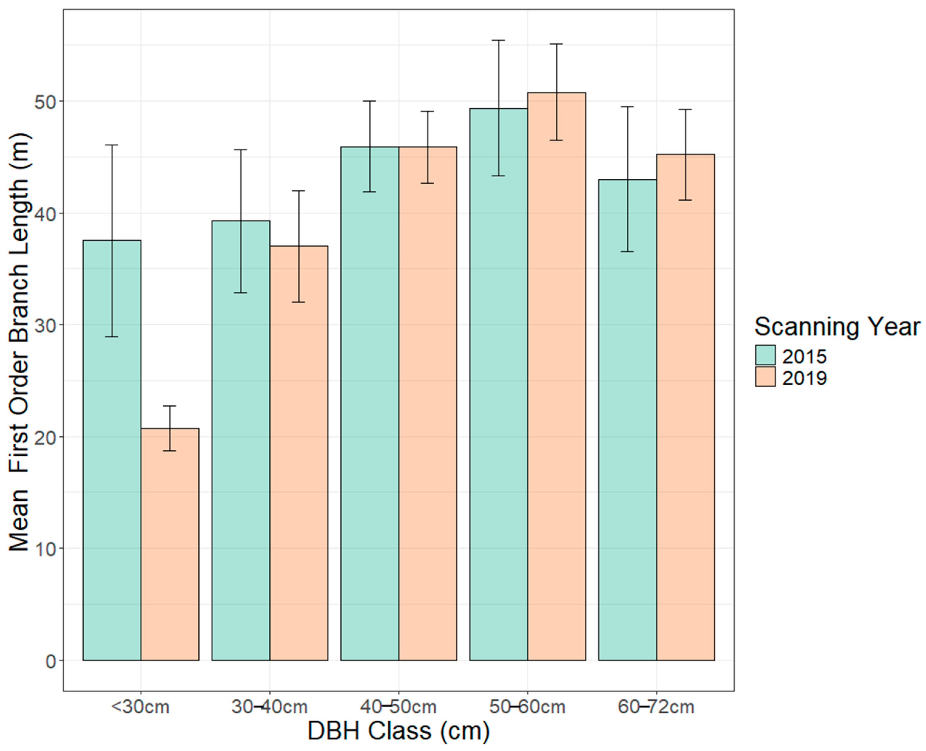
The 53 matched trees were divided into different DBH classes. We used a t-test to compare the differences in the means per tree structural parameter. There were significant differences observed in the means per dbh class for the tree structural parameters, DBH and trunk volume for trees in the dbh class 30–40 cm, whilst significant changes were also observed in the dbh class 50–60 cm for tree height and 30–40 cm and 40–50 cm for the crown area, see Figure 7, Figure 8, Figure 9 and Figure 10 and Table 4, Table 5, Table 6 and Table 7. No significant change was observed in the smallest trees (dbh < 30 cm) and in the largest trees (dbh = 60–72 cm), for the tree parameters, dbh, tree height, crown area and trunk volume suggesting small/negligible change in the small and large trees over the 4 years. For the diameter class 60–72 cm, there was an increase in the means from 2015 to 2019 for the tree structural parameters, DBH, tree height, crown area and trunk volume, indicating small growth in the large trees.
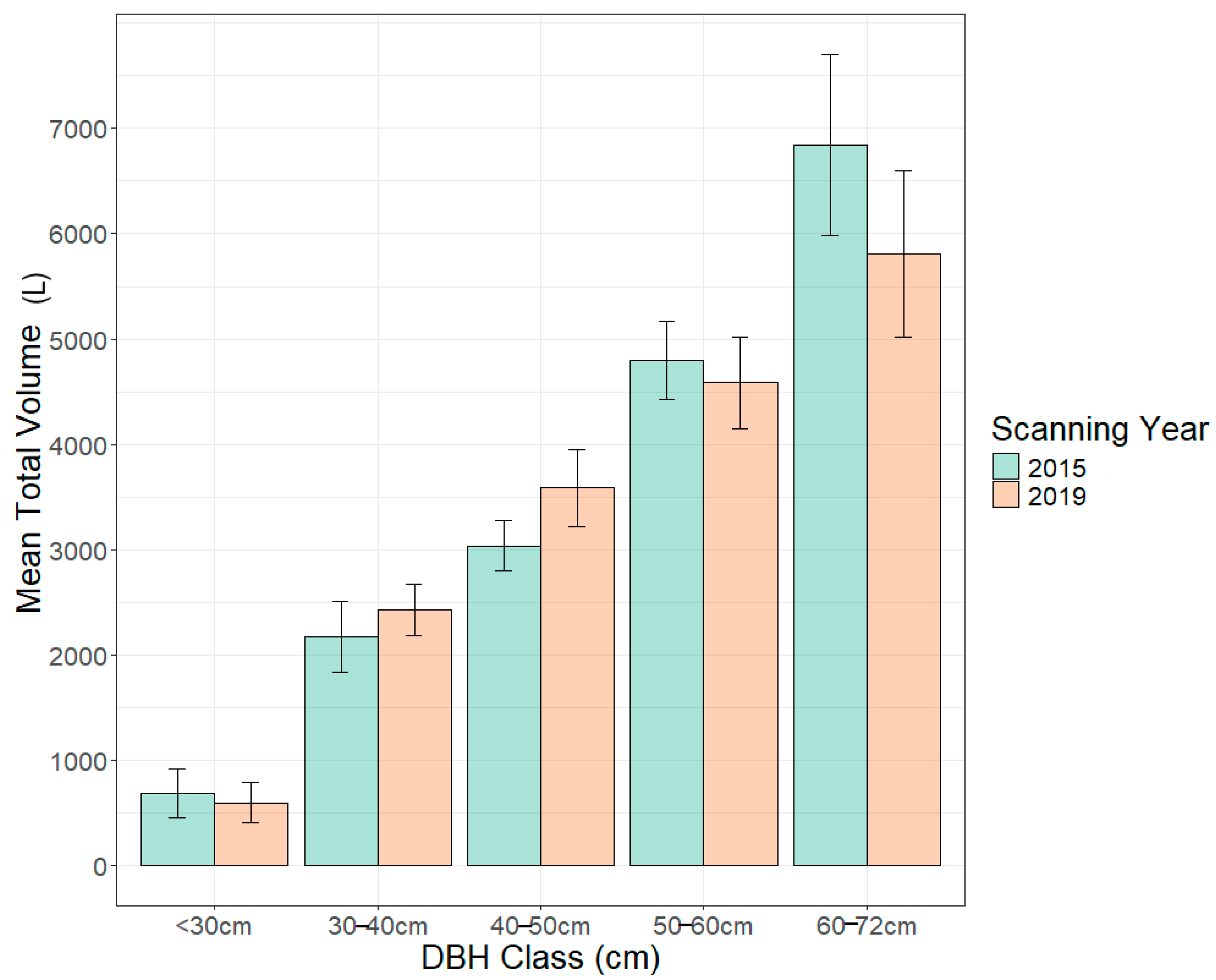
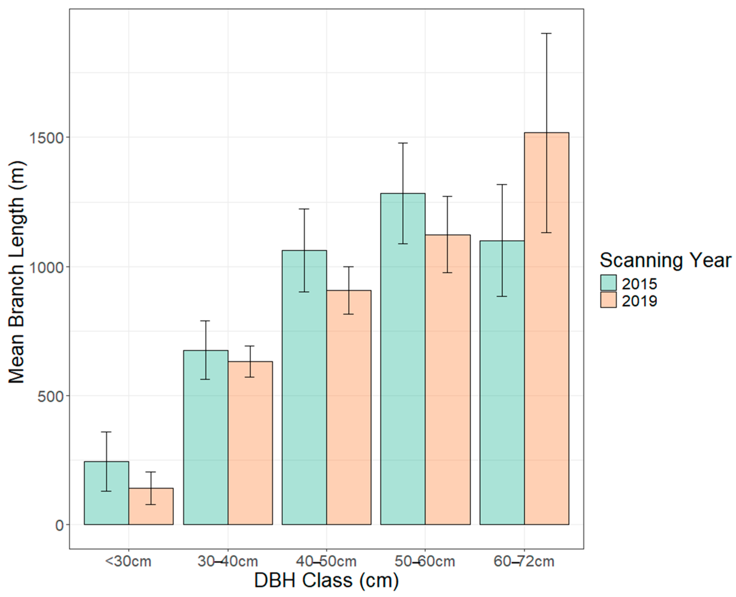
Tree structural parameters of total volume and branch volume showed significant differences in trees in the dbh classes 40–50 cm and 60–72 cm. There was a gain in total and branch volume for trees in the dbh classes, 30–40 cm and 40–50 cm, whilst there was a loss in total and branch volume in the classes <30 cm, 50–60 cm, and 60–72 cm, Figure 11 and Figure 12 and Table 8 and Table 9. Branch length and 1st-order branch length showed no significant differences among the means, indicating no significant change in branch length over the two scanning periods, Figure 13 and Figure 14 and Table 10 and Table 11. For the tree parameter, branch length, a loss in mean branch length was observed for all diameter classes except the very large trees (60–72 cm), implying that the large trees managed to retain most of their branches despite the drought and elephant damage. For the 1st-order branch length, generally, the mean 1st-order branch length is higher for the year 2019 for the diameter classes (>40 cm), indicating that even though trees lost their branches, most retained the main branches with the smallest trees (<30 cm) being mostly affected.

3.5. Comparison of TLS-Measured and Field-Measured DBH

The DBH derived from the TLS using QSMs was compared with the DBH measured in the field for the 38 trees. The TLS-derived DBH showed a positive linear relationship with the field-measured DBH, especially for the scanning year 2019, using linear regression (Figure 15). For the scanning year 2019, the R2 was 0.79 with an RMSE of 6 cm, whilst for 2015, the R2 was 0.71, with an RMSE of 7 cm.

4. Discussion

4.1. Use of Multi-Temporal TLS to Quantify Savanna Tree Structural Change

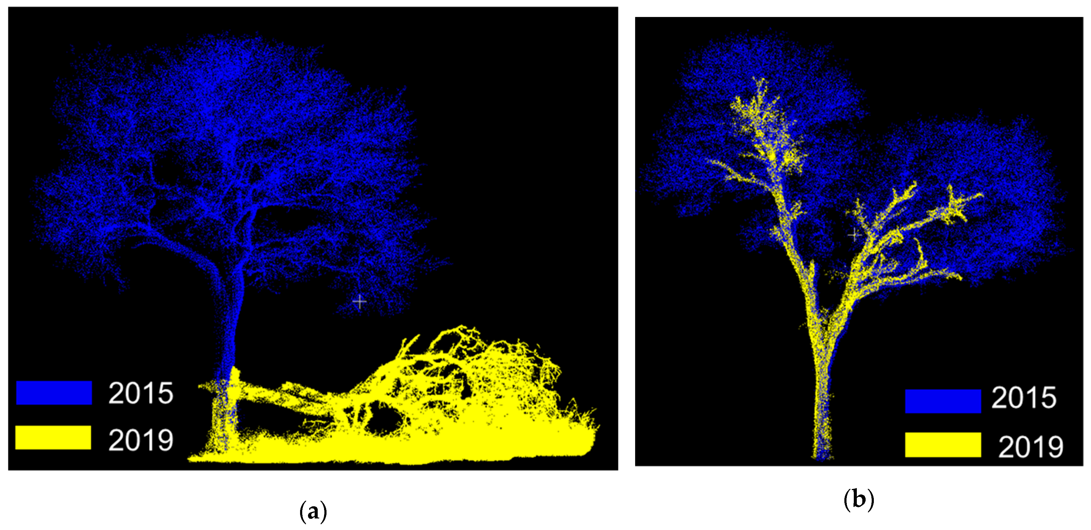
The objective of this study was to quantify changes in tree structure using multi-temporal TLS and discuss the drivers of these changes. We utilized multi-temporal TLS data sets collected in 2015 and 2019, respectively, to quantify the observed changes across eight tree structural parameters. Our analysis revealed a quantifiable loss of trees over two scanning periods (see Figure 5). Regarding the drivers of this change, we identified a total of 75 trees affected by either elephant damage (89%) or drought (11%) using multi-temporal TLS. Additionally, we also identified the corresponding trees that remained standing in 2015 (see Figure 2c) and the total loss in volume (branch + trunk volume) was quantified to be 83.4 m3. Figure 16a,b below illustrate an example of a tree damaged by the effects of herbivory (elephant damage) and one that succumbed to drought effects.
Our results indicate that we can utilize multi-temporal TLS to quantify changes in tree structure over four years. Among the eight tree structural parameters analyzed, significant changes (at the 95% confidence level) were observed in DBH, tree height, crown area, and trunk volume within the DBH class (30–40 cm). Additionally, significant changes were noted in the DBH classes of 40–50 cm (for crown area, total volume, and branch volume) and 60–72 cm (for total and branch volume) (see Figure 7, Figure 8, Figure 9, Figure 10, Figure 11 and Figure 12 and Table 4, Table 5, Table 6, Table 7, Table 8 and Table 9). By accounting for variations in scanning resolutions and positions, we successfully quantified the differences in tree structural parameters. Previous studies [41,42,43] have reported tree structural changes resulting from drought and elephant damage/herbivory, indicating that such changes are a natural phenomenon within ecosystems. Galiano et al. 2012 [44] conducted a study on the effects of drought on the crown conditions and the depletion of carbon reserves in a holm oak forest, finding that 73.8% of the trees exhibited crown damage, which corresponded to a decline in carbon reserves. Thornley et al. 2020 [20] also noted that elephant damage is more severe during the drought periods, concluding that drought conditions increased crown damage in small trees under 4 m, led to higher mortality rates in trees over 6 m, and resulted in severe damage to trees between 4 and 6 m in height. Elephant damage was particularly evident in larger trees over 4 m, with extensive damage observed in the crowns of these trees [20].
No significant changes were observed in branch and 1st-order branch length (see Figure 13 and Figure 14 and Table 10 and Table 11). Although minor changes were noted, they were not statistically significant. A study conducted in a boreal forest [8] reported relatively small changes in tree structural attributes over a short period based on multi-temporal scans taken over five growing seasons. This finding is consistent with the results of the current study, which observed similar trends in branch length over a four-year growing season. Additionally, minor changes over time in the crowns because of normal tree growth were also documented in oil palm trees [45]. The non-significant changes and large RMSEs observed in the branch and 1st order branch length may be attributed to the quality of the point clouds, as uncertainty increases when estimating complex tree parameters, such as branch length, using QSMs.

4.2. Effect of Point Density and QSM Modelling on Accurate Extraction of Tree Parameters and Change Estimation

The differences in these data acquisition methodologies between the scanning periods (see Table 1) were assessed by calculating the relative difference in the number of points per tree across each of the 53 matched trees (see Figure 4). We found that QSMs are highly sensitive to the quality of the point cloud, which primarily impacts the derivation of the more complex tree parameters such as total volume, branch volume, branch and 1st-order branch length. Our observations indicated that a greater disparity in point density between the scanning periods correlates with a larger difference in the computed parameters (see Figure 6e–h). Notably, the standard deviation of 10 reconstructions for the length of 1st-order branches was significantly larger compared with all other computed tree structural parameters (see Figure 6h). When evaluating the relationships among the derived tree structural parameters, we observed that the weakest correlations and largest errors were associated with branch length parameters (see Table 3).
Figure 1 illustrates the distribution of scan positions for the 2015 and 2019 scanning periods within the matched tree area. The 2019 campaign included a greater number of scan positions compared with the 2015 campaign, with scans conducted at different resolutions of 0.025° and 0.015°, respectively. Additionally, the 2019 campaign exhibited a more uniform distribution of the scan positions in the matched tree area than the 2015 campaign. The number of scan positions combined with the scanning resolution and distribution of scan positions in the study area affects the number of points on the matched trees and, therefore, the forest structural parameter under investigation. This affects the reliability of the observed results because differences in point densities between scanning periods affect the co-registration accuracy, which leads to errors when detecting changes in the tree structure, especially for complex tree parameters such as volume and branch length. Hopkins et al. [46] and Duncanson and Dubayah [47] highlighted these limitations when estimating tree structural parameters with multi-temporal lidar data, also observing the precise alignment of the point clouds as a challenge and uncertainty in repeatable parameter estimation given the variation in the lidar acquisitions. Thus, the even distribution of scan positions in both campaigns and ensuring similar data acquisition methodologies is critical in guaranteeing reliability. This was emphasized by Torralba et al. [48], who observed that in addition to the number of scan positions, specific scan distributions improve the accuracy of the derived forest parameter. In addition, Bogdanovich et al. [7] highlighted the need to consider trees that have complete coverage in both scans to avoid uncertainties related to different data acquisition methodologies. In the case of this study, discrepancies between the campaigns were problematic to overcome and thus the decreased number of matched trees.
Low point density leads to an incomplete vegetation structure, which affects the reliability of the assessed parameters, as demonstrated in this study. This is particularly relevant for detecting volumetric changes and parameters related to coverage, such as those derived from the canopy, including branch volume and length. Sumnall et al. [49] noted that parameters related to coverage were more sensitive to the point density (less than 20 points/m2) compared with parameters such as DBH, tree height, and basal area. This finding was further supported by Torralba et al. [48], who observed that high-density TLS are often redundant for height parameters. The variations in point density account for the errors reported in this study regarding complex tree parameters, including total and branch volume as well as branch length, which require comprehensive coverage of the tree for accurate tree reconstruction. Conversely, the negligible errors observed for DBH, tree height, crown area, and trunk volume indicate that the accurate extraction of these tree parameters is not significantly affected by point cloud density.
The QSM modelling technique has limitations because of its random nature, and the derived parameters represent averages across multiple QSMs with an inherent uncertainty [50]. The reliability of each derived parameter is assessed by calculating the sensitivity of each reconstructed tree. Sensitivity is influenced by point density, with trees exhibiting the lowest point densities showing the highest sensitivity [51]. Another inherent limitation of the QSMs arises from the inaccuracies of TLS in resolving small branches, leading to an overestimation of branch volume [52]. This issue was evident in this study, as indicated by the large RMSE error obtained for trees with high (RMSE = 1112 L) and very high (959 L) relative differences in the number of points for the computed branch volume between the two scanning periods (see Figure 6f). Additionally, the distance of the scanner from the tree impacts point density; point density decreases rapidly as the distance from the scanner increases, which is particularly detrimental for small trees [53,54]. Morhart et al. [55] also noted that as distance increases, point cloud density and branch length decrease while branch volume increases. Similar observations were made in the study regarding branch length (see Figure 6g), where trees with a high and very high relative difference exhibited the largest RMSEs of 618 m and 581 m, respectively.
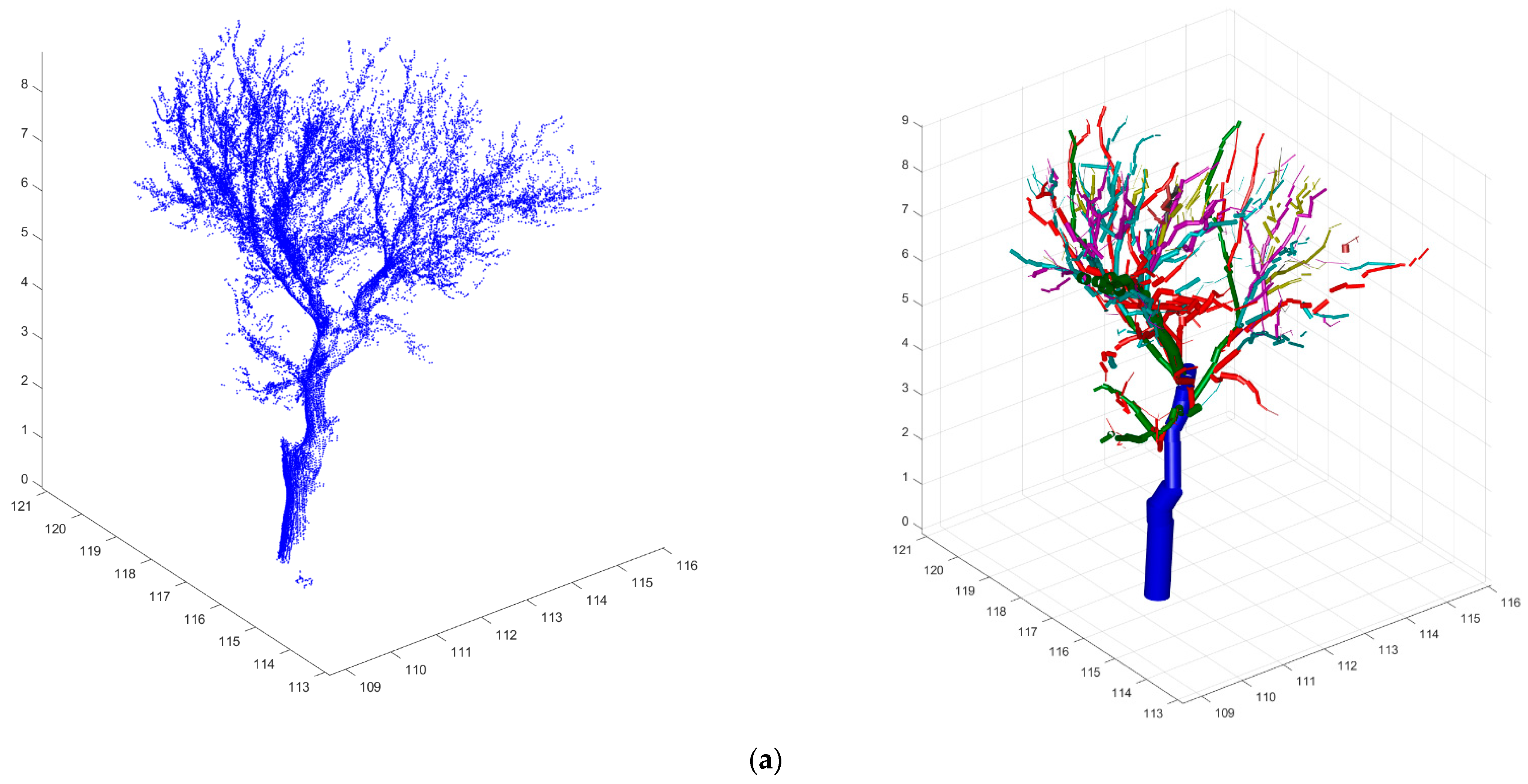
Abegg et al. 2021 [53] recommended the use of high-resolution, high-density TLS scans when tree reconstruction is intended. Due to occlusions and low scan resolutions, the uncertainty in these point cloud data is significant for small branches. The differences in the data acquisition methodologies between the 2015 and 2019 campaigns, combined with modelling errors from the QSMs, lead to the propagation of the errors, thereby compromising the reliability of the observed results. This is particularly true for complex tree parameters such as total volume, branch volume, and branch length. Figure 17a,b below illustrates an example of a matched tree between the two campaigns, which exhibited a high relative difference (50–75%) in the number of points and their resulting QSMs.

4.3. Validation of TLS-Derived Parameters with Field Measurements

In this study, field measurements could not be conducted simultaneously with the TLS campaigns and were instead taken in September 2024. Only 38 of the 53 matched trees could be identified in the field, as some were either dead or missing at the time of measurement. DBH measured in the field was compared with the DBH measured with the QSMs (see Figure 15). Several studies have compared the field-measured DBH with TLS-measured DBH, reporting RMSEs of less than 3 cm [7,15,56,57]. Our study deviates from these results because of the time lag between the TLS and field measurements, resulting in observed RMSE values of 6 cm and 7 cm for the years 2019 and 2015, respectively.

4.4. Future Outlook

Characterizing tree structural parameters over time is critical for savanna ecosystems, as they are dynamic and influenced by various biotic and abiotic factors. The use of multi-temporal TLS and QSMs is essential for the accounting of gains and losses, significantly reducing the time required for fieldwork [15]. In this study, we successfully quantified changes over four years for eight structural parameters. We also assessed tree volume loss and identified trees that succumbed to drought and elephant damage. However, we acknowledge limitations in the TLS acquisitions between the two time periods, particularly regarding the distribution of scan positions in the study area, scan resolution, and the total number of scan positions. These factors affected the point density of the matched trees, resulting in substantial deviations in the computed parameters, especially the complex tree parameters derived from the QSM. Nevertheless, parameters such as DBH, tree height, crown area, and trunk volume were successfully computed with limited uncertainty.
To address the limitations, TLS campaigns for multi-temporal analysis should ensure that trees are fully covered from all angles in both TLS campaigns. This approach helps mitigate the uncertainties introduced by variations in data acquisition methodologies and occlusions [7,58]. Furthermore, it is essential to maintain a high scan resolution with an even distribution of scan positions across the campaigns if reconstruction is intended as a method for deriving the forest structural parameters. This ensures that small branches in the tree crown are not overestimated [48,53].
We also observed that there is a statistically significant change in tree structural parameters over a short growing season of four years. This indicates that even minor changes in tree structure and growth can be successfully quantified with multi-temporal TLS, a finding that has also been reported in other studies. Our research confirms the importance of conducting multi-temporal TLS studies in savannas within short growing seasons, as these ecosystems are dynamic. Small changes resulting from drought, herbivory and fire can be effectively monitored. In this study, we accounted for the effects of the 2015 drought and elephant damage on tree growth. Thus, multi-temporal TLS ensures accurate accounting of tree loss and gain, which is essential for the effective management of these ecosystems. Additionally, Yrttimaa et al. 2020 [8] highlighted that short monitoring periods have been employed to investigate the changes in tree structure using multi-temporal TLS because of the novelty of the methodology.

5. Conclusions

In this study, we quantified structural changes in savanna trees using multi-temporal TLS data and QSMs over four years. We have drawn the following conclusions:
We analyzed the changes in eight tree structural parameters and observed significant variations across different DBH classes, with the exception of branch length and 1st-order branch length. Minor changes in the tree structure within each DBH class were detectable, indicating that even slight alterations in tree structure can be effectively quantified using multi-temporal TLS and QSMs.
The loss of trees between the two TLS campaigns was quantified to 75 trees, and modelling with QSMs estimated the total volume loss (branch + trunk) to be 83.4 m3.
45% of the trees in 2015 were identified as felled or damaged in 2019 because of drought (11%) and elephant damage (89%).
DBH and crown area are strong predictors of tree volume. This was evidenced by the high positive correlations and low RMSEs observed between DBH, crown area, with volume parameters.
Differences in point density and scan resolutions affected the reliability of the parameters derived from the QSMs, particularly for complex tree parameters such as total volume, branch volume, and branch length. The highest calculated residuals were observed in the matched trees exhibiting a high (50–75%) and very high (> 75%) relative difference.
The difference in point density difference is negligible for tree parameters such as DBH, tree height, crown area, and trunk volume. The reported errors for these parameters remain relatively low, regardless of the variation in the number of points associated with the matched trees.
This study demonstrates that the integration of multi-temporal TLS together with QSMs enables precise quantification of structural gains and losses resulting from various interacting drivers. Furthermore, employing TLS in conjunction with QSMs reduces the need for extensive fieldwork, allowing for rapid assessments following an event. This methodology supports the monitoring of both minor and significant structural changes in trees over time, which is beneficial for the management of these dynamic ecosystems.

Author Contributions

T.P.M.: conceptualization, methodology, data processing and analysis, writing—original draft. J.B.: conceptualization, TLS data acquisition and pre-processing, reviewing and editing. P.R.: methodology, software, reviewing and editing. C.C.: field data collection, reviewing and editing. J.S.: conceptualization, reviewing and editing. C.S.: conceptualization, supervision. All authors have read and agreed to the published version of the manuscript.

Funding

This study was made possible by funding from the Deutscher Akademischer Austauschdienstenst (DAAD) Ref No. SPACES II.2 CaBuDe 57531823 to T.P. Muumbe and the Bundesministerium für Bildung und Forschung (BMBF) through the projects ArsAfrica, South African Land Degradation Monitor (SALDi, Grant No. 01LL1701A), and Ecosystem Management Support for Climate Change in Southern Africa (EMSAfrica, Grant No. 01LL1801D). Funding to P. Raumonen was provided by the Research Council of Finland: Flagship of Advanced Mathematics for Sensing Imaging and Modelling, Grant 359185; Centre of Excellence of Inverse Modelling and Imaging, Grant 353090. Fieldwork in Kruger National Park was conducted under the SANParks research permit KNP Erosion, Ref. No. BAAJ1127. We acknowledge support from the German Research Foundation (DFG) Project number 512648189 and the Open Access Publication Fund of the Thueringer Universitaets- und Landesbibliothek Jena.

Data Availability Statement

Data presented in this study are available on request from (jussi.baade@uni-jena.de). These data are not publicly available due to the study being carried out in a protected area.

Acknowledgments

We acknowledge the support of South African National Parks (SANParks) Scientific Services in Skukuza and Game Guards during fieldwork in the Kruger National Park.

Conflicts of Interest

The authors declare no conflicts of interest.

References

  1. Grace, J.; José, J.S.; Meir, P.; Miranda, H.S.; Montes, R.A. Productivity and carbon fluxes of tropical savannas. J. Biogeogr. 2006, 33, 387–400. [Google Scholar] [CrossRef]
  2. Higgins, S.I.; Bond, W.J.; Trollope, W.S.W. Fire, resprouting and variability: A recipe for grass-tree coexistence in savanna. J. Ecol. 2000, 88, 213–229. [Google Scholar] [CrossRef]
  3. McCleery, R.; Monadjem, A.; Baiser, B.; Fletcher, R.; Vickers, K.; Kruger, L. Animal diversity declines with broad-scale homogenization of canopy cover in African savannas. Biol. Conserv. 2018, 226, 54–62. [Google Scholar] [CrossRef]
  4. Levick, S.R.; Asner, G.P. The rate and spatial pattern of treefall in a savanna landscape. Biol. Conserv. 2013, 157, 121–127. [Google Scholar] [CrossRef]
  5. Stevens, N.; Erasmus, B.F.N.; Archibald, S.; Bond, W.J. Woody encroachment over 70 years in South African savannahs: Overgrazing, global change or extinction aftershock? Philos. Trans. R. Soc. B Biol. Sci. 2016, 371, 20150437. [Google Scholar] [CrossRef]
  6. Urban, M.; Heckel, K.; Berger, C.; Schratz, P.; Smit, I.P.J.; Strydom, T.; Baade, J.; Schmullius, C. Woody cover mapping in the savanna ecosystem of the Kruger National Park using sentinel-1 C-band time series data. Koedoe 2020, 62, a1621. [Google Scholar] [CrossRef]
  7. Bogdanovich, E.; Perez-Priego, O.; El-Madany, T.S.; Guderle, M.; Pacheco-Labrador, J.; Levick, S.R.; Moreno, G.; Carrara, A.; Pilar Martín, M.; Migliavacca, M. Using terrestrial laser scanning for characterizing tree structural parameters and their changes under different management in a Mediterranean open woodland. For. Ecol. Manag. 2021, 486, 118945. [Google Scholar] [CrossRef]
  8. Yrttimaa, T.; Luoma, V.; Saarinen, N.; Kankare, V.; Junttila, S.; Holopainen, M.; Hyyppä, J.; Vastaranta, M. Structural changes in Boreal forests can be quantified using terrestrial laser scanning. Remote Sens. 2020, 12, 2672. [Google Scholar] [CrossRef]
  9. Demol, M.; Verbeeck, H.; Gielen, B.; Armston, J.; Burt, A.; Disney, M.; Duncanson, L.; Hackenberg, J.; Kükenbrink, D.; Lau, A.; et al. Estimating forest above-ground biomass with terrestrial laser scanning: Current status and future directions. Methods Ecol. Evol. 2022, 13, 1628–1639. [Google Scholar] [CrossRef]
  10. Sheppard, J.; Morhart, C.; Hackenberg, J.; Spiecker, H. Terrestrial laser scanning as a tool for assessing tree growth. iForest 2017, 10, 172–179. [Google Scholar] [CrossRef]
  11. Xu, D.; Wang, H.; Xu, W.; Luan, Z.; Xu, X. LiDAR applications to estimate forest biomass at individual tree scale: Opportunities, challenges and future perspectives. Forests 2021, 12, 550. [Google Scholar] [CrossRef]
  12. Raumonen, P.; Kaasalainen, M.; Åkerblom, M.; Kaasalainen, S.; Kaartinen, H.; Vastaranta, M.; Holopainen, M.; Disney, M.; Lewis, P.; Markku, Å.; et al. Fast Automatic Precision Tree Models from Terrestrial Laser Scanner Data. Remote Sens. 2013, 5, 491–520. [Google Scholar] [CrossRef]
  13. Liang, X.; Hyyppä, J.; Kaartinen, H.; Holopainen, M.; Melkas, T. Detecting changes in forest structure over time with bi-temporal terrestrial laser scanning data. ISPRS Int. J. Geo-Inf. 2012, 1, 242–255. [Google Scholar] [CrossRef]
  14. Englhart, S.; Jubanski, J.; Siegert, F. Quantifying Dynamics in Tropical Peat Swamp Forest Biomass with Multi-Temporal LiDAR Datasets. Remote Sens. 2013, 5, 2368–2388. [Google Scholar] [CrossRef]
  15. Srinivasan, S.; Popescu, S.C.; Eriksson, M.; Sheridan, R.D.; Ku, N.W. Multi-temporal terrestrial laser scanning for modeling tree biomass change. For. Ecol. Manag. 2014, 318, 304–317. [Google Scholar] [CrossRef]
  16. Kaasalainen, S.; Krooks, A.; Liski, J.; Raumonen, P.; Kaartinen, H.; Kaasalainen, M.; Puttonen, E.; Anttila, K.; Mäkipää, R. Change detection of tree biomass with terrestrial laser scanning and quantitative structure modelling. Remote Sens. 2014, 6, 3906–3922. [Google Scholar] [CrossRef]
  17. Luck, L.; Kaestli, M.; Hutley, L.B.; Calders, K.; Levick, S.R. Reduced model complexity for efficient characterisation of savanna woodland structure using terrestrial laser scanning. Int. J. Appl. Earth Obs. Geoinf. 2023, 118, 103255. [Google Scholar] [CrossRef]
  18. Qi, Y.; Coops, N.C.; Daniels, L.D.; Butson, C.R. Comparing tree attributes derived from quantitative structure models based on drone and mobile laser scanning point clouds across varying canopy cover conditions. ISPRS J. Photogramm. Remote Sens. 2022, 192, 49–65. [Google Scholar] [CrossRef]
  19. Urban, M.; Berger, C.; Mudau, T.E.; Heckel, K.; Truckenbrodt, J.; Odipo, V.O.; Smit, I.P.J.; Schmullius, C. Surface moisture and vegetation cover analysis for drought monitoring in the southern Kruger National Park using Sentinel-1, Sentinel-2, and Landsat-8. Remote Sens. 2018, 10, 1482. [Google Scholar] [CrossRef]
  20. Thornley, R.; Spencer, M.; Zitzer, H.R.; Parr, C.L. Woody vegetation damage by the African elephant during severe drought at Pongola Game Reserve, South Africa. Afr. J. Ecol. 2020, 58, 658–673. [Google Scholar] [CrossRef]
  21. Smit, I.P.J.; Asner, G.P.; Govender, N.; Kennedy-Bowdoin, T.; Knapp, D.E.; Jacobson, J. Effects of Fire and Herbivory on the Stability of Savanna Ecosystems. Ecol. Appl. 2010, 84, 1865–1875. [Google Scholar] [CrossRef] [PubMed]
  22. Scheiter, S.; Higgins, S.I. Impacts of climate change on the vegetation of Africa: An adaptive dynamic vegetation modelling approach. Glob. Chang. Biol. 2009, 15, 2224–2246. [Google Scholar] [CrossRef]
  23. Osborne, C.P.; Charles-Dominique, T.; Stevens, N.; Bond, W.J.; Midgley, G.; Lehmann, C.E.R. Human impacts in African savannas are mediated by plant functional traits. New Phytol. 2018, 220, 10–24. [Google Scholar] [CrossRef]
  24. Sankaran, M.; Ratnam, J.; Hanan, N. Woody cover in African savannas: The role of resources, fire and herbivory. Glob. Ecol. Biogeogr. 2008, 17, 236–245. [Google Scholar] [CrossRef]
  25. Foxcroft, L.C.; Richardson, D.M.; Rejmánek, M.; Pyšek, P. Alien plant invasions in tropical and sub-tropical savannas: Patterns, processes and prospects. Biol. Invasions 2010, 12, 3913–3933. [Google Scholar] [CrossRef]
  26. Scholes, R.J.; Gureja, N.; Giannecchinni, M.; Dovie, D.; Wilson, B.; Davidson, N.; Piggott, K.; McLoughlin, C.; Van der Velde, K.; Freeman, A.; et al. The environment and vegetation of the flux measurement site near Skukuza, Kruger National Park. Koedoe 2001, 44, 73–84. [Google Scholar] [CrossRef]
  27. Dyer, C. New names for the African Acacia species in Vachellia and Senegalia. South. For. 2014, 76, iii. [Google Scholar] [CrossRef]
  28. MacFadyen, S.; Zambatis, N.; Van Teeffelen, A.J.A.; Hui, C. Long-term rainfall regression surfaces for the Kruger National Park, South Africa: A spatio-temporal review of patterns from 1981 to 2015. Int. J. Climatol. 2018, 38, 2506–2519. [Google Scholar] [CrossRef]
  29. Sankaran, M. Droughts and the ecological future of tropical savanna vegetation. J. Ecol. 2019, 107, 1531–1549. [Google Scholar] [CrossRef]
  30. Scholes, R.J.; Archer, S.R. Tree-grass interactions in Savannas. Annu. Rev. Ecol. Syst. 1997, 28, 517–544. [Google Scholar] [CrossRef]
  31. Rice, K.J.; Matzner, S.L.; Byer, W.; Brown, J.R. Patterns of tree dieback in Queensland, Australia: The importance of drought stress and the role of resistance to cavitation. Oecologia 2004, 139, 190–198. [Google Scholar] [CrossRef] [PubMed]
  32. O’Brien, M.J.; Engelbrecht, B.M.J.; Joswig, J.; Pereyra, G.; Schuldt, B.; Jansen, S.; Kattge, J.; Landhäusser, S.M.; Levick, S.R.; Preisler, Y.; et al. A synthesis of tree functional traits related to drought-induced mortality in forests across climatic zones. J. Appl. Ecol. 2017, 54, 1669–1686. [Google Scholar] [CrossRef]
  33. Greenwood, S.; Ruiz-Benito, P.; Martínez-Vilalta, J.; Lloret, F.; Kitzberger, T.; Allen, C.D.; Fensham, R.; Laughlin, D.C.; Kattge, J.; Bönisch, G.; et al. Tree mortality across biomes is promoted by drought intensity, lower wood density and higher specific leaf area. Ecol. Lett. 2017, 20, 539–553. [Google Scholar] [CrossRef] [PubMed]
  34. RIEGL Laser Measurements Systems. RIEGL VZ-1000 High-Resolution and Accurate 3D Measurements. Data Sheet. 2017, pp. 1–4. Available online: http://www.riegl.com/uploads/tx_pxpriegldownloads/DataSheet_VZ-1000_2017-06-14.pdf (accessed on 4 December 2024).
  35. Dong, Y.; Fan, G.; Zhou, Z.; Liu, J.; Wang, Y.; Chen, F. Low cost automatic reconstruction of tree structure by adqsm with terrestrial close-range photogrammetry. Forests 2021, 12, 1020. [Google Scholar] [CrossRef]
  36. Li, W.; Guo, Q.; Jakubowski, M.K.; Kelly, M. A new method for segmenting individual trees from the lidar point cloud. Photogramm. Eng. Remote Sens. 2012, 78, 75–84. [Google Scholar] [CrossRef]
  37. Raumonen, P.; Casella, E.; Calders, K.; Murphy, S.; Åkerbloma, M.; Kaasalainen, M. Massive-Scale Tree Modelling From Tls Data. ISPRS Ann. Photogramm. Remote Sens. Spat. Inf. Sci. 2015, 2, 189–196. [Google Scholar] [CrossRef]
  38. The R Project for Statistical Computing. 2024. Available online: http://www.r-project.org (accessed on 4 December 2024).
  39. Munna, A.H.; Amuri, N.A.; Hieronimo, P.; Woiso, D.A. The right tree in the right place: Predicting and mapping global-scale suitable areas for Marula tree, Sclerocarya birrea, (A. Rich.) Horchst, subspecies cultivation, conservation, and use in restoring global drylands. Front. Biogeogr. 2023, 15, 1–15. [Google Scholar] [CrossRef]
  40. Munna, A.H.; Amuri, N.A.; Hieronimo, P.; Woiso, D.A. Modelling ecological niches of Sclerocarya birrea subspecies in Tanzania under the current and future climates. Silva Fenn. 2023, 57, 23009. [Google Scholar] [CrossRef]
  41. Martínez-Vilalta, J.; Lloret, F. Drought-induced vegetation shifts in terrestrial ecosystems: The key role of regeneration dynamics. Glob. Planet. Chang. 2016, 144, 94–108. [Google Scholar] [CrossRef]
  42. Ben-Shahar, R. Patterns of elephant damage to vegetation in northern Botswana. Biol. Conserv. 1993, 65, 249–256. [Google Scholar] [CrossRef]
  43. Clark, J.S.; Iverson, L.; Woodall, C.W.; Allen, C.D.; Bell, D.M.; Bragg, D.C.; D’Amato, A.W.; Davis, F.W.; Hersh, M.H.; Ibanez, I.; et al. The impacts of increasing drought on forest dynamics, structure, and biodiversity in the United States. Glob. Chang. Biol. 2016, 22, 2329–2352. [Google Scholar] [CrossRef] [PubMed]
  44. Galiano, L.; Martínez-Vilalta, J.; Sabaté, S.; Lloret, F. Determinants of drought effects on crown condition and their relationship with depletion of carbon reserves in a Mediterranean holm oak forest. Tree Physiol. 2012, 32, 478–489. [Google Scholar] [CrossRef]
  45. Husin, N.A.; Khairunniza-Bejo, S.; Abdullah, A.F.; Kassim, M.S.M.; Ahmad, D. Multi-temporal analysis of terrestrial laser scanning data to detect basal stem rot in oil palm trees. Precis. Agric. 2022, 23, 101–126. [Google Scholar] [CrossRef]
  46. Hopkinson, C.; Chasmer, L.; Hall, R.J. The uncertainty in conifer plantation growth prediction from multi-temporal lidar datasets. Remote Sens. Environ. 2008, 112, 1168–1180. [Google Scholar] [CrossRef]
  47. Duncanson, L.; Dubayah, R. Monitoring individual tree-based change with airborne lidar. Ecol. Evol. 2018, 8, 5079–5089. [Google Scholar] [CrossRef] [PubMed]
  48. Torralba, J.; Carbonell-Rivera, J.P.; Ruiz, L.Á.; Crespo-Peremarch, P. Analyzing TLS Scan Distribution and Point Density for the Estimation of Forest Stand Structural Parameters. Forests 2022, 13, 2115. [Google Scholar] [CrossRef]
  49. Sumnall, M.J.; Albaugh, T.J.; Carter, D.R.; Cook, R.L.; Hession, W.C.; Campoe, O.C.; Rubilar, R.A.; Wynne, R.H.; Thomas, V.A. Effect of varied unmanned aerial vehicle laser scanning pulse density on accurately quantifying forest structure. Int. J. Remote Sens. 2022, 43, 721–750. [Google Scholar] [CrossRef]
  50. Kükenbrink, D.; Gardi, O.; Morsdorf, F.; Thürig, E.; Schellenberger, A.; Mathys, L. Above-ground biomass references for urban trees from terrestrial laser scanning data. Ann. Bot. 2021, 128, 709–724. [Google Scholar] [CrossRef] [PubMed]
  51. Muumbe, T.P.; Singh, J.; Baade, J.; Raumonen, P.; Coetsee, C.; Thau, C.; Schmullius, C. Individual Tree-Scale Aboveground Biomass Estimation of Woody Vegetation in a Semi-Arid Savanna Using 3D Data. Remote Sens. 2024, 16, 399. [Google Scholar] [CrossRef]
  52. Morales, A.; Macfarlane, D.W. Reducing tree volume overestimation in quantitative structure models using modeled branch topology and direct twig measurements. For. Int. J. For. Res. 2024, cpae046. [Google Scholar] [CrossRef]
  53. Abegg, M.; Boesch, R.; Schaepman, M.E.; Morsdorf, F. Impact of Beam Diameter and Scanning Approach on Point Cloud Quality of Terrestrial Laser Scanning in Forests. IEEE Trans. Geosci. Remote Sens. 2021, 59, 8153–8167. [Google Scholar] [CrossRef]
  54. Kankare, V.; Puttonen, E.; Holopainen, M.; Hyyppä, J. The effect of TLS point cloud sampling on tree detection and diameter measurement accuracy. Remote Sens. Lett. 2016, 7, 495–502. [Google Scholar] [CrossRef]
  55. Morhart, C.; Schindler, Z.; Frey, J.; Sheppard, J.P.; Calders, K.; Disney, M.; Morsdorf, F.; Raumonen, P.; Seifert, T. Limitations of estimating branch volume from terrestrial laser scanning. Eur. J. For. Res. 2024, 143, 687–702. [Google Scholar] [CrossRef]
  56. Huang, H.; Li, Z.; Gong, P.; Cheng, X.; Clinton, N.; Cao, C.; Ni, W.; Wang, L. Automated methods for measuring DBH and tree heights with a commercial scanning lidar. Photogramm. Eng. Remote Sens. 2011, 77, 219–227. [Google Scholar] [CrossRef]
  57. Liu, G.; Wang, J.; Dong, P.; Chen, Y.; Liu, Z. Estimating individual tree height and diameter at breast height (DBH) from terrestrial laser scanning (TLS) data at plot level. Forests 2018, 9, 398. [Google Scholar] [CrossRef]
  58. Campos, M.B.; Litkey, P.; Wang, Y.; Chen, Y.; Hyyti, H.; Hyyppä, J.; Puttonen, E. A Long-Term Terrestrial Laser Scanning Measurement Station to Continuously Monitor Structural and Phenological Dynamics of Boreal Forest Canopy. Front. Plant Sci. 2021, 11, 606752. [Google Scholar] [CrossRef] [PubMed]
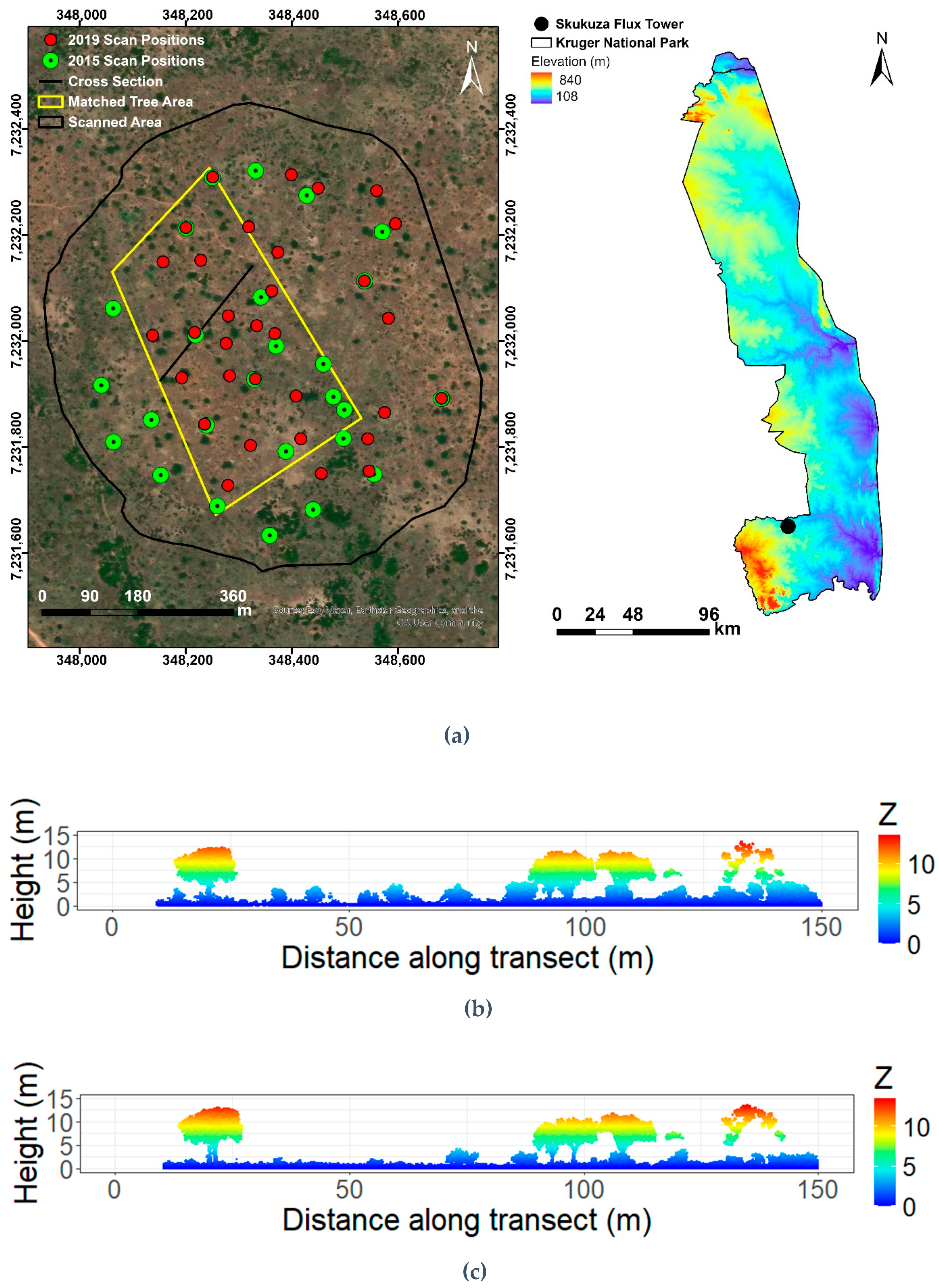
Figure 1. Study area location (left) showing the scanned area marked in black and the matched tree area marked in yellow and (right) the map of Kruger National Park showing the location of Skukuza Flux Tower where scanning was conducted (a) showing a cross-section displaying the change in vegetation over the 4-year period (b) 2015 and (c) 2019.
Remotesensing 17 00757 g001
Figure 2. Number of correctly segmented trees (a) 178 trees segmented in 2015 (b) 168 trees segmented in 2019, 93 standing and 75 felled or damaged (c) 75 damaged in 2019 matched to standing trees in 2015.
Remotesensing 17 00757 g002
Figure 3. The location of the 53 matched trees in the study area.
Remotesensing 17 00757 g003
Figure 5. Canopy Height Models Differences (a) 2019 CHM (b) 2015 CHM (c) Δ CHM = 2019 CHM-2015 CHM.
Remotesensing 17 00757 g005
Figure 6. Comparison between tree parameters between the two scanning periods (a) DBH (b) Tree Height (c) Crown Area (d) Trunk Volume (e) Total Volume (f) Branch Volume (g) Branch Length and (h) Branch length 1st-order branches. The dashed line is the 1:1 line, and the grey area represents the 95% confidence interval, while the black solid line represents the linear regression between the tree structural parameters in 2019 and 2015. n = 53. The error bars indicate the standard deviation of 10 reconstructions.
Remotesensing 17 00757 g006aRemotesensing 17 00757 g006bRemotesensing 17 00757 g006c
Figure 7. Mean DBH in DBH Classes.
Remotesensing 17 00757 g007
Figure 8. Mean Tree Height in DBH Classes.
Remotesensing 17 00757 g008
Figure 9. Mean Crown Area in DBH Classes.
Remotesensing 17 00757 g009
Figure 10. Mean Trunk Volume in DBH Classes.
Remotesensing 17 00757 g010
Figure 11. Mean Total Volume in DBH Classes.
Remotesensing 17 00757 g011
Figure 12. Mean Branch Volume in DBH Classes.
Remotesensing 17 00757 g012
Figure 13. Mean Branch Length in DBH Classes.
Remotesensing 17 00757 g013
Figure 14. Mean 1st-order Branch Length in DBH Classes.
Remotesensing 17 00757 g014
Figure 15. Comparison between the TLS-derived and the field-measured DBH for 38 trees for both scanning periods. The dashed line is the 1:1 line, and the grey area represents the 95% confidence interval, while the blue and red solid lines represent the linear regression between the TLS-measured and field-measured DBH for 2015 and 2019, respectively.
Remotesensing 17 00757 g015
Figure 16. (a) An example of a tree that succumbed to the effects of elephant damage. The image shows the trees standing in 2015 (blue), and on the ground in 2019 (yellow) (b) An example of a tree that succumbed to the effects of drought—the image shows the tree with a crown in 2015 (blue) and having lost most of its crown in 2019 (yellow).
Remotesensing 17 00757 g016
Figure 17. Example of a matched tree that had a high relative difference (50–75%) in the number of points (a) The tree in 2015 and the resulting QSM model (51 200 points) (b) The tree in 2019 and the resulting QSM Model (115 700 points).
Remotesensing 17 00757 g017aRemotesensing 17 00757 g017b
Table 1. Scan settings used when scanning in 2015 and 2019, respectively.
20152019
Scan Positions3032
Beam divergence0.3 mrad0.3 mrad
Pulse repetition rate300 kHz (450 m)300 kHz (450 m)
Angular Sampling0.015°0.025°
Table 2. Tree structural parameters measured.
Tree Structural ParameterUnit of
Measurement
Definition
Diameter at breast height
(DBH)
Tree height
Crown area
Trunk volume
Total volume
Branch volume
Branch length
1st-order branch length
cm

m
m2
L
L
L
m
m
The diameter of the cylinder fitted to the height (1.1–1.5 m)

Height of the tree
Area of the crown’s planar projection’s convex hull
The volume of the tree stem
The total volume of the tree
The volume of all the branches
The total length of all the branches
Total length of the main branches
Table 3. Comparison among the derived parameters.
20152019
PredictorResponseR2RMSER2RMSE
DBHTree Height0.368.6 m0.378.6 m
DBHCrown area0.7885.2 m20.8191.1 m2
DBHTrunk vol0.91883 L0.91913 L
DBHTotal vol0.793576 L0.793657 L
DBHBranch vol0.732662 L0.702702 L
DBHBranch len0.54908.3 m0.68891.9 m
DBHBranch len (1st)0.0736.8 m0.2537.2 m
Tree heightCrown area0.4280.6 m20.4585.3 m2
Tree heightTrunk vol0.52839 L0.57868 L
Tree heightTotal vol0.433360 L0.483460 L
Tree heightBranch vol0.392490 L0.412537 L
Tree heightBranch len0.38894.3 m0.35822.3 m
Tree heightBranch len (1st)0.3038.3 m0.5739.0 m
Crown areaTrunk vol0.75863 L0.77897 L
Crown areaTotal vol0.813656 L0.843756 L
Crown areaBranch vol0.792765 L0.812825 L
Crown areaBranch len0.65955.7 m0.84948.7 m
Crown areaBranch len (1st)0.0936.9 m0.3437.7 m
Trunk volTotal vol0.853672 L0.833742 L
Trunk volBranch vol0.772732 L0.722751 L
Trunk volBranch len0.54916 m0.65892.5 m
Trunk volBranch len (1st)0.1537.3 m0.4138.0 m
Total volBranch vol0.993066 L0.983010 L
Total volBranch len0.721005.1 m0.78940.8 m
Total volBranch len (1st)0.2437.9 m0.5038.5 m
Branch volBranch len0.731017.9 m0.78947.0 m
Branch volBranch len (1st)0.2538.0 m0.4938.5 m
Branch lenBranch len (1st)0.3438.6 m0.3337.7 m
DBH is Diameter at Breast Height, vol refers to the trunk, total and branch volume, len refers to the total branch length or total length of the 1st-order branches (branch len 1st).
Table 4. Comparison of DBH in different DBH Classes.
ParameterDBH
Class cm (n)
2015 DBH
Mean ± SE
2019 DBH
Mean ± SE
p Value
DBH (cm)<30 (4)18 ± 2.7 19 ± 2.6 0.83
30–40 (15)37 ± 0.6 38 ± 1.1 0.05 *
40–50 (15)46 ± 0.8 46 ± 1.0 1
50–60 (14)53 ± 0.8 52 ± 1.10.07
60–72
(5)
63 ± 1.9 63 ± 2.5 0.72
* indicates significant differences at 95%.
Table 5. Comparison of Tree Height bin different DBH Classes.
ParameterDBH
Class cm (n)
2015 TH
Mean ± SE
2019 TH
Mean ± SE
p Value
Tree Height (m)<30 (4)8.6 ± 1.0 8.3 ± 0.9 0.24
30–40 (15)10.3 ± 0.4 10.5 ± 0.4 0.09
40–50 (15)11.4 ± 0.3 11.2 ± 0.3 0.16
50–60 (14)11.8 ± 0.4 12.0 ± 0.40.02 *
60–72 (5) 11.6 ± 0.4 11.7 ± 0.4 0.42
* indicates significant differences at 95%.
Table 6. Comparison of Crown Area in different DBH Classes.
ParameterDBH
Class cm (n)
2015 CA
Mean ± SE
2019 CA
Mean ± SE
p Value
Crown Area (m2)<30 (4)14.5 ± 4.5 15.2 ± 4.5 0.77
30–40 (15)62.6 ± 3.8 66.1 ± 3.7 0.007 *
40–50 (15)86.2 ± 4.9 94.0 ± 6.3 0.04 *
50–60 (14)112.1 ± 10.8 117.5 ± 11.8 0.07
60–72 (5)136.7 ± 21.3 140.3 ± 20.9 0.16
* indicates significant differences at 95%.
Table 7. Comparison of Trunk Volume in different DBH Classes.
ParameterDBH
Class cm (n)
2015 TrV
Mean ± SE
2019 TrV
Mean ± SE
p Value
Trunk Volume (L)<30 (4)175 ± 78 160 ± 60 0.68
30–40 (15)528 ± 39 586 ± 38 0.002 *
40–50 (15)792 ± 29 811 ± 39 0.38
50–60 (14)1117 ± 64 1138 ± 72 0.41
60–72 (5)1523 ± 136 1559 ± 176 0.61
* indicates significant differences at 95%.
Table 8. Comparison of Total Volume in different DBH Classes.
ParameterDBH
Class cm (n)
2015 ToV
Mean ± SE
2019 ToV
Mean ± SE
p Value
Total Volume (L)<30 (4)684 ± 234591 ± 1920.42
30–40 (15)2170 ± 341 2426 ± 240 0.17
40–50 (15)3032 ± 2393584 ± 3700.007 *
50–60 (14)4797 ± 367 4583 ± 4340.43
60–72 (5)6842 ± 861 5809 ± 7930.04 *
* indicates significant differences at 95%.
Table 9. Comparison of Branch Volume in different DBH Classes.
ParameterDBH
Class cm (n)
2015 BrV
Mean ± SE
2019 BrV
Mean ± SE
p Value
Branch Volume (L)<30 (4)509 ± 211431 ± 1840.44
30–40 (15)1642 ± 3051839 ± 2110.27
40–50 (15)2240 ± 2272774 ± 345 0.007 *
50–60 (14)3679 ± 3303444 ± 3970.37
60–72 (5)5319 ± 8054250 ± 7560.04 *
* indicates significant differences at 95%.
Table 10. Comparison of Branch Length in different DBH Classes.
ParameterDBH
Class cm (n)
2015 BrL
Mean ± SE
2019 BrL
Mean ± SE
p Value
Branch Length (m)<30 (4)244 ± 114140 ± 630.22
30–40 (15)675 ± 113 632 ± 600.64
40–50 (15)1062 ± 161907 ± 92 0.16
50–60 (14)1284 ± 196 1123 ± 1480.32
60–72 (5)1101 ± 218 1518 ± 3860.09
Table 11. Comparison of 1st-order Branch Length in different DBH Classes.
ParameterDBH
Class cm (n)
2015 LBO
Mean ± SE
2019 LBO
Mean ± SE
p Value
1st-order Branch Length (m)<30 (4)38 ± 921 ± 20.19
30–40 (15)39 ± 6 37 ± 50.42
40–50 (15)46 ± 446 ± 3 0.98
50–60 (14)49 ± 6 51 ± 40.68
60–72 (5)43 ± 645 ± 40.59
Disclaimer/Publisher’s Note: The statements, opinions and data contained in all publications are solely those of the individual author(s) and contributor(s) and not of MDPI and/or the editor(s). MDPI and/or the editor(s) disclaim responsibility for any injury to people or property resulting from any ideas, methods, instructions or products referred to in the content.