Multisource Precipitation Data Merging Using a Dual-Layer ConvLSTM Model

Abstract

Precipitation is a key component of the water cycle. Different precipitation data sources have strengths and weaknesses. To combine these strengths and achieve accurate precipitation data, this study introduces a dual-layer neural network (D-ConvLSTM) based on a convolutional long short-term memory neural network (ConvLSTM) that integrates ground station data (1 h interval) and grid precipitation data generated by the China Meteorological Administration Multi-source merged Precipitation Analysis System (CMPAS, 1 h interval, 0.05° × 0.05°) through a two-layer network for precipitation identification and correction. To evaluate the performance of the proposed model, D-ConvLSTM, optimal interpolation (OI), and a single-layer ConvLSTM model are evaluated in the Dadu River Basin, China. The results show that D-ConvLSTM outperforms the CMPAS in all the metrics compared with the OI and ConvLSTM, with improvements of 18.9% and 19.8% in the critical success index (CSI) and Kling–Gupta efficiency (KGE), respectively. D-ConvLSTM enhances gridded precipitation under various conditions, including areas without station data, different intensities, and regions. Furthermore, this study analyzes the impact of training data distribution on the performance of the D-ConvLSTM model and enhances model performance by adjusting the training data distribution. The analysis reveals that the ratio of dry to wet data in the training set affects the model’s identification performance. The ratio of overestimation to underestimation of gridded data compared with station observations influences value correction. This study offers a new model for merging station and gridded precipitation data and provides insights for enhancing the accuracy of neural network merging.

1. Introduction

Precipitation is a crucial component of the water cycle [1,2]. Accurate and reliable precipitation observations help to better understand and simulate hydrometeorological processes, aiding in informed decision-making and risk assessment for natural and human environments [3,4,5,6].

Methods for precipitation observations include ground observations, radar monitoring, and satellite retrieval [7,8,9], and each method has strengths and weaknesses. Ground stations provide accurate precipitation data at the point scale but have limited spatial coverage depending on the distribution of stations [10,11]. In contrast, satellite and radar data cover larger areas and better represent spatial distributions but have accuracy limitations due to cloud cover, surface conditions, and algorithm limitations [12,13,14]. Various precipitation datasets have been developed based on these observations, such as the Global Historical Climatology Network (GHCN), which includes data from more than 100,000 stations across 180 countries [15]; the Global Precipitation Climatology Centre (GPCC), which provides gridded data based on observations [16]; the Tropical Rainfall Measuring Mission (TRMM), which combines multiple sensors [17]; and the ERA5 reanalysis precipitation products [18]. These datasets serve as valuable tools for research and operational applications; however, many studies have revealed that bias still exists in precipitation datasets [19,20,21].

To further improve the accuracy and reliability of precipitation datasets, one promising approach is to integrate different information to better utilize the advantages of multisource precipitation, i.e., precipitation merging [22,23,24,25]. Many scholars have researched multisource precipitation merging technologies and have proposed various new methods [26,27]. Conventional approaches, such as objective analysis [28] and optimal interpolation [29,30], achieve multisource precipitation merging by correcting the constructed initial fields. Other merging methods, such as geographically weighted regression [31,32] and kriging interpolation [33], incorporate auxiliary information from the underlying surface. However, most conventional methods rely on strong assumptions [34], such as the assumption that the data are stationary on a global or local scale and that the relationship between the data is linear [35,36,37]. In operational applications, when real conditions do not conform to these assumptions, the performance of these conventional methods is reduced [38,39].

Machine learning technologies can learn complex patterns and relationships between different data, making them preferable for data merging [40,41,42,43]. With the development of machine learning technologies, many studies have attempted to leverage the powerful feature extraction and learning capabilities of machine learning algorithms for multisource precipitation merging. Nguyen et al. used a random forest algorithm to merge multiple satellite precipitation products in South Korea [44], Kumar et al. employed various machine learning algorithms, including support vector machine (SVM), to integrate station and satellite observational data [45], and Wehbe et al. used artificial neural networks (ANNs) to merge multiple precipitation products from the Arabian Peninsula [46]. To account for the spatial and temporal characteristics of precipitation, some scholars have further utilized neural networks such as convolutional neural networks (CNNs) [47,48] and long short-term memory (LSTM) neural networks [49,50] for multisource precipitation merging. Among neural network algorithms, the ConvLSTM network inherits the advantages of both CNNs and LSTMs, enabling it to capture the spatiotemporal features of precipitation data simultaneously. Many studies have applied ConvLSTM to multisource precipitation merging, and their merged results also show that fully considering the spatiotemporal relationship of precipitation can improve the accuracy of merged precipitation data [39,51,52,53].

However, the above methods do not consider the precipitation identification error, which is also one of the significant sources of precipitation bias. For example, Tian et al. and Lei et al. conducted error analysis on grid precipitation data and reported that missed and misreported precipitation errors are important components of precipitation errors [54,55]. Moreover, errors in precipitation identification affect the identification of the spatial location and scope of precipitation [56], the length of the dry/wet moment, and the statistics of the start/end time [57]. Accurately determining whether precipitation events occur is crucial for improving the performance of grid-observed precipitation. Therefore, some studies have introduced separate identification modules for multisource precipitation merging. For example, Lei et al. constructed a precipitation identification module using various methods, such as gradient boosting decision tree (GBDT), extreme gradient boosting (XGBoost), and random forest (RF) [56]. Zhang et al. used methods such as SVM, RF, ANN, and extreme learning machine (ELM) for precipitation identification [58]. Lyu et al. used XGBoost for precipitation identification [59], and Li et al. identified precipitation by constructing a gridded precipitation probability estimation model [57]. The inclusion of these precipitation identification modules further reduced the errors in precipitation merging.

However, the precipitation identification modules constructed using these methods usually require stretching and dimensionality reduction to convert two-dimensional spatial data into one-dimensional data before they are input into the model for calculation, which can compromise the spatial characteristics of precipitation [60,61]. ConvLSTM can directly utilize two-dimensional spatial data, allowing for a more comprehensive consideration of the spatiotemporal characteristics of precipitation. To the best of our knowledge, current studies that use ConvLSTM for multisource precipitation merging have not considered precipitation identification. Additionally, for machine learning, the distribution of sample data can significantly affect model performance [62,63,64]. Moreover, most current studies that use machine learning for multisource precipitation data merging have explored only the impact of sample dataset size on model performance, without analyzing how various distributions of precipitation sample data influence the merged results [56,57]. These limitations affect the accuracy of precipitation merging.

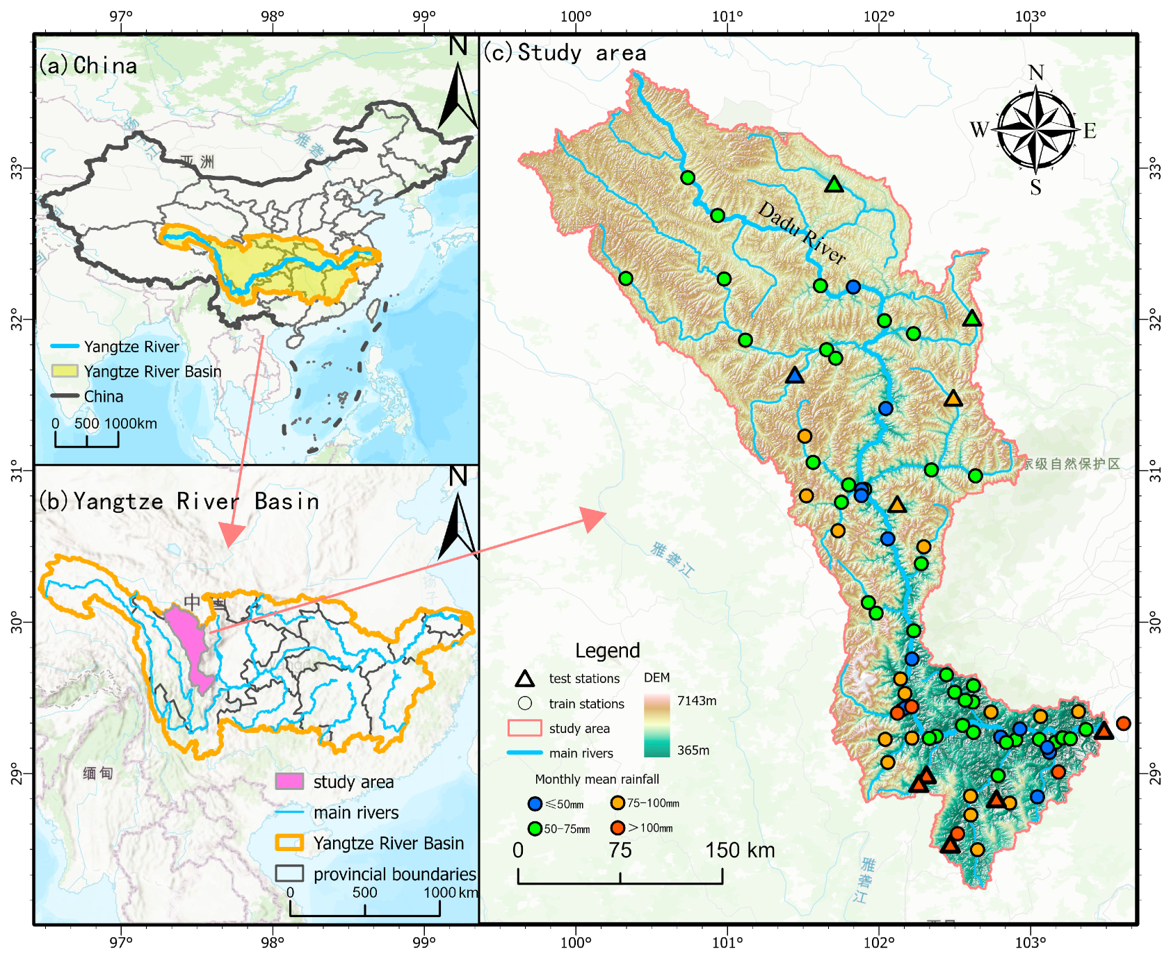
To address these limitations, we propose a dual-layer neural network based on ConvLSTM (D-ConvLSTM) for merging ground station and gridded precipitation data. The first layer is the precipitation identification ConvLSTM module, which comprehensively considers the spatial distribution characteristics of precipitation and uses cross-entropy [65] as the loss function to achieve a dry‒wet classification. The second layer uses the mean absolute error (MAE) as the loss function to correct precipitation values during wet periods. It is applied to the Dadu River Basin in China and compared with the traditional optimal interpolation method and single-layer ConvLSTM, verifying the effectiveness and advantages of D-ConvLSTM. Additionally, we change the ratio of dry to wet data in the training set of the precipitation identification network (ConvLSTM-identify) and the ratio of overestimated or underestimated CMPAS precipitation values compared to station observation values in the training set of the precipitation correction network (ConvLSTM-correct) to explore the impact of the training data distribution on the performance of the neural network merging model.

2. Study Area and Data

2.1. Study Area

The Dadu River (DDR, Figure 1) originates from the southern foothills of the Guoluo Mountains in Qinghai Province and is the largest tributary of the Minjiang River [66]. The area of the DDR is approximately 77,400 km² and has a slightly ‘L’-shaped configuration, with higher terrain in the northwest and lower terrain in the southeast [67]. The average annual precipitation across the DDR is approximately 800 mm, increasing from the northwest to the southeast of the basin [68]. The DDR is characterized by complex terrain and diverse landforms; therefore, it is significantly influenced by both the East Asian and South Asian monsoons. The upper DDR has a plateau mountain climate with relatively low annual precipitation and fewer days of heavy rainfall. In contrast, the middle and lower reaches experience a subtropical humid monsoon climate with higher annual precipitation and more days of intense rainfall in summer [69,70].

2.2. Data

2.2.1. Station Precipitation Data

This paper uses observed precipitation data from 82 stations, of which 33 are hydrological stations and 49 are precipitation stations. The spatial distribution of stations is shown in Figure 1, with the number of stations increasing gradually from upstream to downstream, and the stations with higher precipitation values are mainly located downstream. The time range of the collected station data is from 7 August 2018 08:00:00 to 21 September 2022 11:00:00, with a temporal resolution of 1 h. The data were collected and quality controlled by the State Energy Dadu River Basin Hydropower Development Co., Ltd.

2.2.2. CMPAS Precipitation Data

The grid precipitation data used in this study are from the CMPAS precipitation data product. The ‘CMPAS China Hourly Precipitation Real-time Merging Analysis Product’ utilizes ground observational data, radar quantitative precipitation estimation, and satellite-derived precipitation data and was developed using key techniques such as bias correction and merging analysis. Overall, the quality of this product is superior to those of similar international products within China [27,71,72]. However, there are still some errors in the grid precipitation in the study area of this paper [73]. It is necessary to further improve the accuracy by multisource precipitation merging. This product covers the Chinese region (0–60°N, 70–140°E) with a spatial resolution of 0.05° × 0.05°. The time range of the data obtained in this study is from 7 August 2018 08:00:00 to 21 September 2022 11:00:00, with a temporal resolution of 1 h. The CMPAS precipitation data used in this study are provided by the State Energy Dadu River Basin hydropower development Co., Ltd. and can also be accessed from the China Meteorological Data Network (https://data.cma.cn/, accessed on 21 September 2022).

2.2.3. Terrain Data

This paper uses Shuttle Radar Topography Mission (SRTM) digital elevation model (DEM) data to quantify the terrain. Because topographic changes play an important role in precipitation [74] and the spatial distribution trend of precipitation in the Dadu River Basin is very similar to that of topographic distribution [67,68], the DEM is chosen as the auxiliary variable in this paper. The SRTM was created by NASA’s Shuttle Radar Topography Mission. The data are sourced from the Geospatial Data Cloud (www.gscloud.cn, accessed on 21 September 2022).

2.2.4. Data Preprocessing

First, a bilinear interpolation tool in the software ArcGIS 10.8 is used to resample DEM data to match the resolution of the CMPAS (0.05°× 0.05°). Then, the dataset used as input for ConvLSTM and D-ConvLSTM is divided, with 10 stations randomly selected as independent test stations. For the remaining 72 stations, the training and validation sets span from 7 August 2018 08:00:00 to 26 June 2021 14:00:00, with 20% of the time randomly selected as the validation set. The test set spans from 26 June 2021 15:00:00 to 21 September 2022 11:00:00.

For ConvLSTM and D-ConvLSTM, the input data at time t are a matrix of size (a + 1, n, n), where a is a hyperparameter of the model used to set the time length for looking back at the precipitation, and n is also a hyperparameter used to set the range of terrain and precipitation extraction around the stations. The entire matrix consists of grid precipitation data and a DEM within the range of n × n from time t to t-a∆t, as shown in Figure 2.

3. Methods

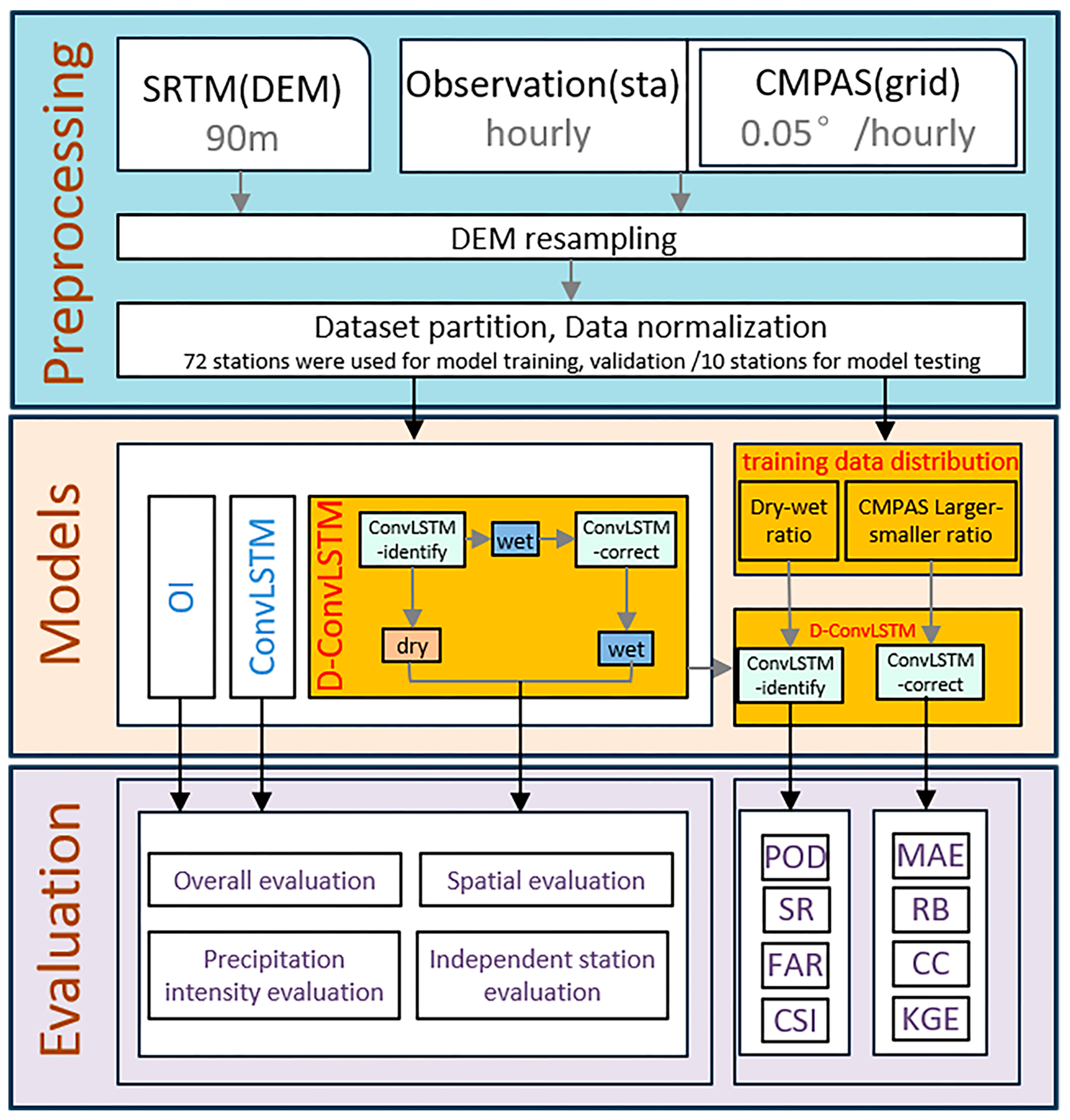
The flowchart of this study is presented in Figure 3. This study proposes the D-ConvLSTM model to integrate observed precipitation data from DDR stations with CMPAS gridded precipitation data, addressing both precipitation classification and value estimation errors. The performance of D-ConvLSTM is assessed using multiple evaluation metrics and compared against the results of the OI and ConvLSTM to demonstrate its overall improvement. Furthermore, the study examines the impact of different training data distributions on the D-ConvLSTM merging model by changing the ratio of dry to wet data in the training data and the proportion of overestimation or underestimation of gridded precipitation compared with station observations. Finally, classification and statistical indicators, including overall evaluation, independent station evaluation, precipitation intensity evaluation, spatial evaluation, and evaluation of D-ConvLSTM model performance with different training data distributions, are used to evaluate different types of merged precipitation.

3.1. ConvLSTM and D-Convlstm

ConvLSTM is a deep learning model that integrates convolutional neural networks (CNNs) and long short-term memory (LSTM) networks. ConvLSTM considers both the temporal correlation of precipitation sequences and the spatial distribution characteristics of precipitation, making it particularly suitable for multisource precipitation data merging [51,52]. Its structure is similar to that of LSTM [75]. To reduce the complexity of the network structure, this paper adopts a simplified ConvLSTM, which has the same structure as LSTM but replaces the Hadamard product in LSTM with convolution operations from neural networks, as shown in Figure 4.

Its internal calculation formula is as follows:

$$\begin{array}{c}{i}_t=\sigma \left(w_{xi}\ast x_t+w_{hi}\ast h_{t-1}+b_i\right)\hfill \\ f_t=\sigma \left(w_{xf}\ast x_t+w_{hf}\ast h_{t-1}+b_f\right)\hfill \\ c_t=f_t \mathrm{o} c_{t-1}+i_t \mathrm{o} tanh\left(w_{xc}\ast x_t+w_{hc}\ast h_{t-1}+b_c\right)\hfill \\ o_t=\sigma \left(w_{xo}\ast x_t+w_{ho}\ast h_{t-1}+b_o\right)\hfill \\ h_t=o_t \mathrm{o} tanh\left(c_t\right)\hfill \end{array}$$

(1)

where $\sigma$ is the sigmoid activation function; $tanh$ is another activation function; $\mathrm{o}$ is the Hadamard product; $\ast$ is the convolution operation in the neural network; $x_t$ is the input at time $t$; $h_t$ is the hidden state at time $t$;$i_t$, $f_t$, $c_t$, and $o_t$ are the input gate, forgetting gate, status gate, and output gate, respectively; and $w$ and $b$ are the weights and bias, respectively.

Based on the work of Lei et al. [56], Zhang et al. [58], and Lyu et al. [59], this study proposes an improved D-ConvLSTM model based on ConvLSTM for the merging of grid precipitation and station-observed precipitation, with the internal structure shown in Figure 5. D-ConvLSTM has two layers. The first layer, ConvLSTM-identify, is used for dry (precipitation = 0) and wet (precipitation > 0) identification. The second layer, ConvLSTM-correct, is used for correcting precipitation values during wet periods. Different loss functions are applied to the two layers mentioned above.

The first layer employs the cross-entropy loss function, which is defined in Equation (2):

$${Loss}_{classify}=-{\displaystyle \frac{1}{N}}\sum _{i=1}^N\left[y_{i}log\left(p_i\right)+\left(1-y_i\right)log\left(1-p_i\right)\right]$$

(2)

where $N$ is the total number of samples; $y_i$ is the category to which sample $i$ belongs; and $p_i$ is the predicted value for sample $i$, represented as a probability value.

The second layer employs the mean absolute error loss function, which is defined as Equation (3):

$${Loss}_{regress}=-{\displaystyle \frac{1}{N}}\sum _{i=1}^N\left|p_i-y_i\right|$$

(3)

where $N$ is the total number of samples; $y_i$ is the category to which sample $i$ belongs; and $p_i$ is the predicted value for sample $i$.

Several hyperparameters need to be determined for training the D-ConvLSTM model. In this study, after multiple adjustments of batch size, hidden size, and learning rate, we found that changes in these three hyperparameters had a minimal impact on the merged results. Considering computer performance, model complexity, and training time, this study used the following parameters: batchSize = 10,000, hiddenSize = 32, and learningRate = 0.01. For n and seqLenth, n was set to (7,9,11,13,15), and seqLenth was set to (4,5,6,7,8), with repeated experiments conducted to select the most suitable hyperparameters. The hyperparameters used by ConvLSTM and D-ConvLSTM are shown in

Table 1. Hyperparameters of ConvLSTM and D-ConvLSTM.

Hyperparameter	Value	Description
n	7	Extraction range of grid data
seqLenth	5	Length of the time series for each sample
batchSize	10,000	Number of samples per batch
hiddenSize	32	Size of the ConvLSTM’s hidden state
learningRate	0.01	Model learning rate

. The computational environment used in this study is configured as follows: the processor is a 12th Gen Intel(R) Core(TM) i7-12700 with 12 cores and 20 threads; the memory is 32 GB; the GPU is an NVIDIA RTX A4000 with 16 GB of VRAM; the operating system is Windows 11; and the deep learning framework used is PyTorch. Training the D-ConvLSTM model for 100 epochs using this environment takes 54 min, while calculating the precipitation for 2881 grids and 36,148 time steps takes 56 min.

3.2. Optimal Interpolation (OI)

Optimal interpolation (OI) is a conventional approach for grid and station precipitation merging and is widely used in many operational systems. The OI is an objective analysis method based on the optimal interpolation theory proposed by Eliassen in 1954 [29]. In this study, we also use the OI as a benchmark for comparison. For each grid point, the OI calculates the analysis value by adding the initial estimate of the grid point to the correction value. The correction value is obtained by weighting the deviations of the observed values from surrounding stations relative to the initial estimate at the station’s location [76]. In this study, when the OI is used for merging, stations located on the interpolated grid are not considered. The calculation principles and formulas can be found in Appendix A.1.

In areas with a dense distribution of study sites, the distances between the nearest neighboring stations range from 5 to 15 km. In this study, when determining the parameters of the OI model, r was set to (5,10,15,20,25), and s was set to (50,75,100,125,150), with repeated experiments conducted.

Table 2. Parameters of the OI used in this study.

Hyperparameter	Value	Description
r	5 km	Initial search radius
Δr	5 km	Search radius growth step
s	50 km	Distance threshold

presents the parameters utilized for the OI model in this study.

3.3. Training Data Selection Strategies

This study also aims to investigate the impact of the training data distribution on the merging performance. For ConvLSTM-identify (1st layer), the strategy is to change the ratio of dry to wet data in the training set. For wet samples, considering that the number of dry samples far exceeds that of wet samples, we make no adjustments to wet samples and use all the data for training. For dry samples, we adjust the samples for training from 2.5% to 100%, increasing by 2.5% each time.

For ConvLSTM-correct (2nd layer), the strategy is to change the ratio of CMPAS precipitation values that are overestimated or underestimated compared with station-observed values. Owing to the samples in this study where precipitation exceeds 5 mm, the CMPAS is generally overestimated, whereas for samples below 5 mm, the CMPAS is typically underestimated. To focus the model more on samples with greater precipitation, no adjustments are made to the samples where CMPAS precipitation values are underestimated during training; all of them are included in model training. For samples with overestimated CMPAS precipitation values, the amounts are increased sequentially from 2.5% to 100%, in increments of 2.5% each time. The specific change strategies are shown in

Table 3. Strategies for changing the training data distribution.

Layer	Strategy	Ratio
ConvLSTM-identify	Change the dry data ratio	(2.5%, 100%, 2.5%)
ConvLSTM-correct	Change the ratio of CMPAS precipitation values that are larger than observed data	(2.5%, 100%, 2.5%)

.

3.4. Evaluation Metrics

We employ different metrics to evaluate the performance of D-ConvLSTM and investigate the influence of training data selection. We also compare the results of D-ConvLSTM with those of ConvLSTM and the OI to identify the strengths and weaknesses of D-ConvLSTM. We calculate the following metrics using station precipitation observations and corresponding grid-merging precipitation values.

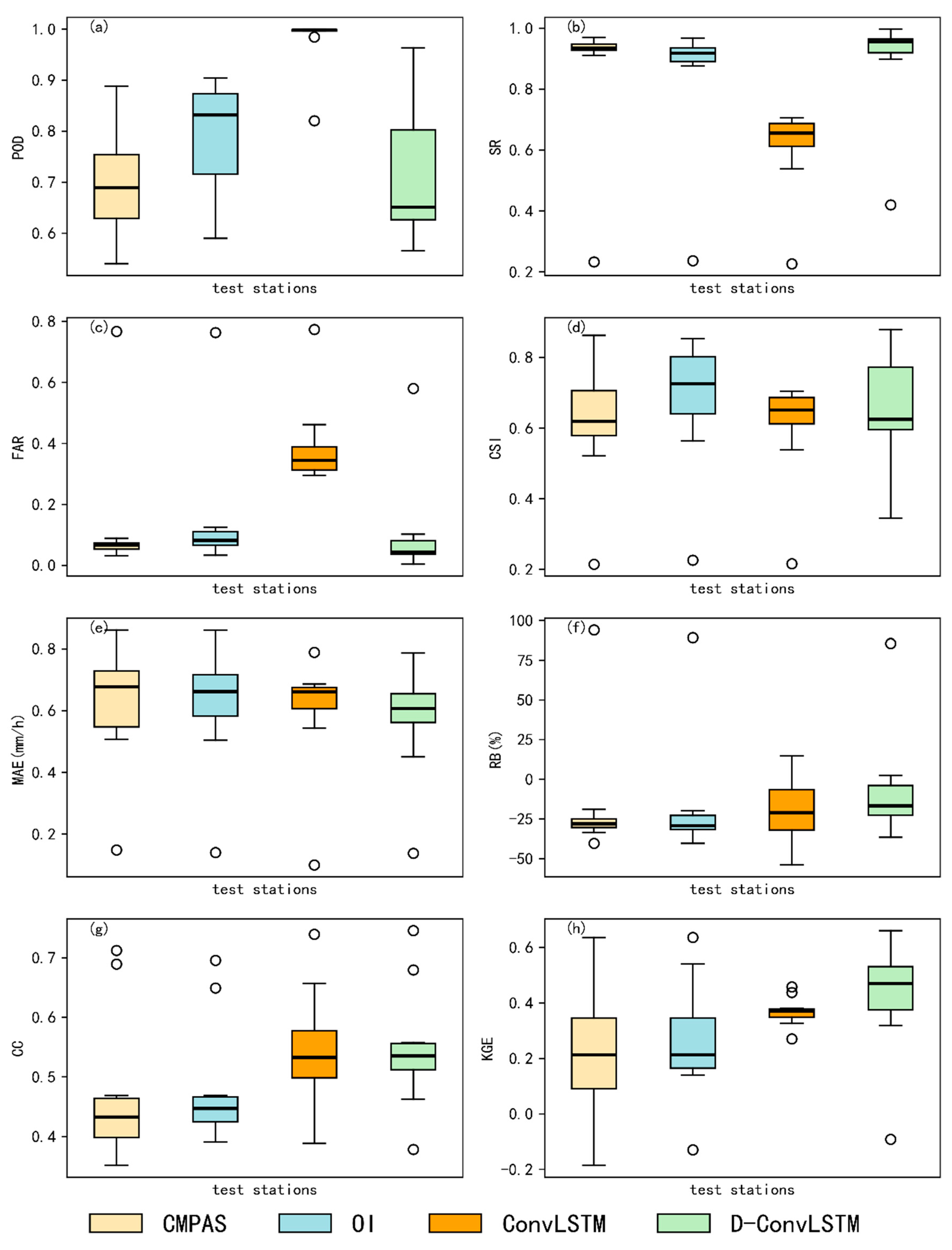
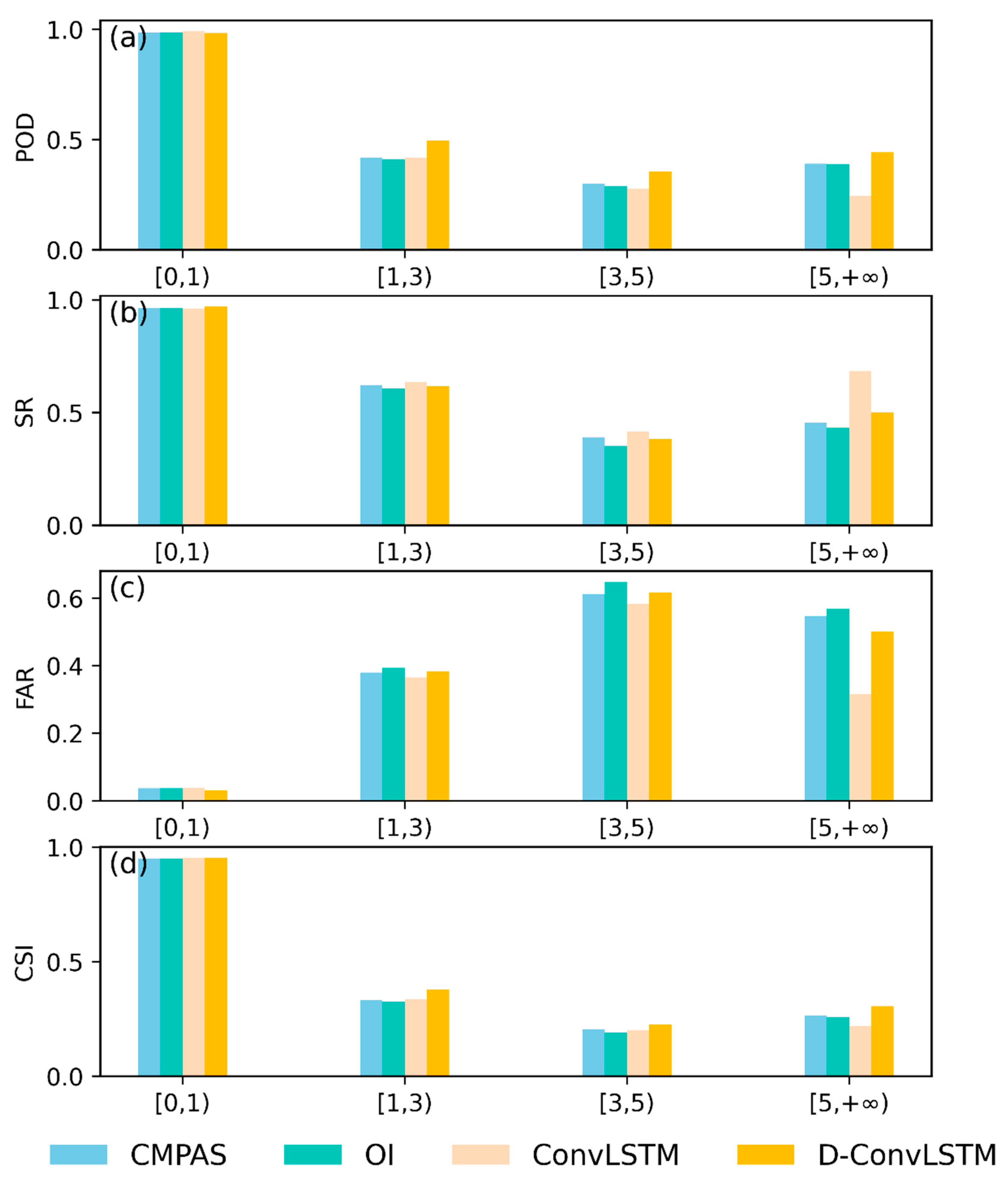
The evaluation metrics include classification metrics and statistical metrics. This study uses classification metrics, including the probability of detection (POD), success ratio (SR), false alarm ratio (FAR), and critical success index (CSI), to assess the model’s precipitation identification capability. The POD indicates the ability to correctly detect precipitation events. The SR and FAR represent the ratios of correctly detected precipitation periods and incorrectly detected precipitation periods to the total detected precipitation periods, respectively. The CSI combines the POD and FAR, serving as a comprehensive indicator of precipitation identification capability. The optimal value of the POD, SR, and CSI is 1, whereas the FAR is 0.

They are defined in Equation (4):

$$\begin{array}{c}POD=H/(H+M)\hfill \\ SR=H/(H+F)\hfill \\ FAR=F/(H+F)\hfill \\ CSI=H/(H+M+F)\hfill \end{array}$$

(4)

where $H$ is the number of periods where precipitation was observed and correctly detected as precipitation; $F$ is the number of periods where precipitation was not observed but incorrectly detected as precipitation; and $M$ is the number of periods where precipitation was observed but incorrectly detected as not occurring.

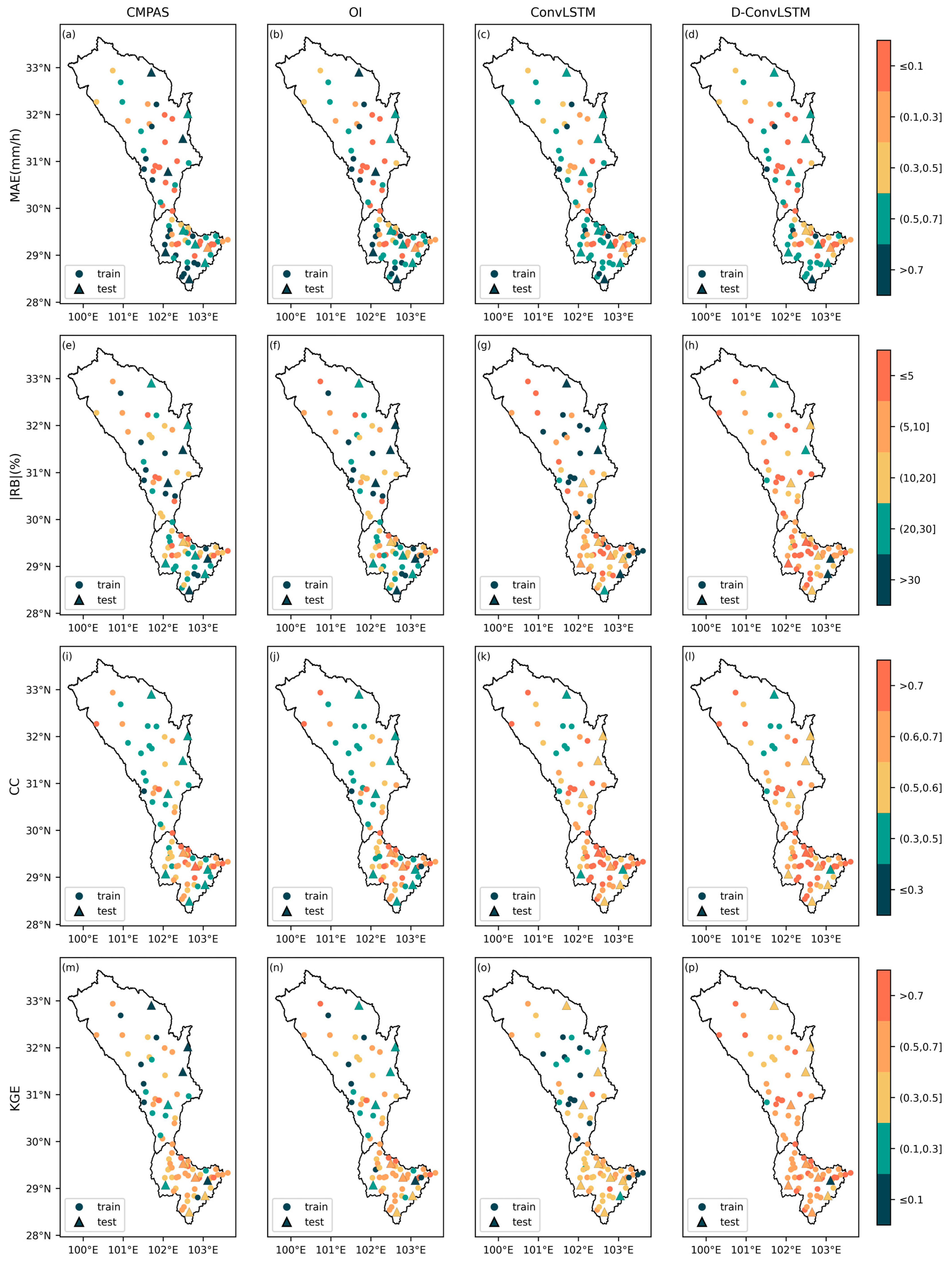
This study uses statistical metrics to assess the estimation errors of merged precipitation values and their alignment with station-observed precipitation. These metrics include the mean absolute error (MAE), relative bias (RB), Pearson correlation coefficient (CC), and Kling–Gupta efficiency (KGE). The MAE quantifies the error between merged precipitation and observed values over short time intervals, whereas the RB captures the cumulative error across extended periods. The CC measures the degree of correlation between merged precipitation and observed values, whereas the KGE evaluates the overall goodness of fit between these two datasets. The optimal value of the CC and KGE is 1, whereas the values of the MAE and RB are 0.

They are defined in Equation (5):

$$\begin{array}{c}MAE={\displaystyle \frac{{\sum }_{i=1}^n\left|P_{ob,i}-P_{s,i}\right|}{n}}\hfill \\ RB={\displaystyle \frac{{\sum }_{i=1}^n\left(P_{s,i}-P_{ob,i}\right)}{{\sum }_{i=1}^n{P}_{ob,i}}}\hfill \\ CC={\displaystyle \frac{{\sum }_{i=1}^n\left(P_{ob,i}-\overline{P_{ob}}\right)\left(P_{s,i}-\overline{P_s}\right)}{\sqrt{{\sum }_{i=1}^n{\left(P_{ob,i}-\overline{P_{ob}}\right)}^2}\sqrt{{\sum }_{i=1}^n{\left(P_{s,i}-\overline{P_s}\right)}^2}}}\hfill \\ KGE=1-\sqrt{{\left(1-CC\right)}^2+{\left(1-\beta \right)}^2+{\left(1-\gamma \right)}^2}, \beta ={\displaystyle \frac{{\mu }_s}{{\mu }_{ob}}}, \gamma ={\displaystyle \frac{{\sigma }_s/{\mu }_s}{{\sigma }_{ob}/{\mu }_{ob}}}\hfill \end{array}$$

(5)

where $n$ is the number of periods; $ob$ is the station observation at time $t$; $s$ is the merged precipitation at time $t$; $\overline{P}$ is the mean precipitation in the entire evaluation period; $\beta$ is the deviation ratio; $\gamma$ is the variation rate; $\mu$ is the mean precipitation in the evaluation period; and $\sigma$ is the standard deviation of precipitation in the evaluation period.

4. Results

4.1. Overall Performance of D-ConvLSTM and Comparison with ConvLSTM and OI

Using observed precipitation data from all the stations, this study calculated the metrics for the baseline (CMPAS) and three merged precipitation datasets (i.e., D-ConvLSTM, ConvLSTM, and OI). All the metrics are shown in

Table 4. All the metrics of CMPAS and the three models’ merged precipitation.

Model	POD	SR	FAR	CSI	MAE (mm/h)	RB (%)	CC	KGE
CMPAS	0.678	0.813	0.187	0.587	0.168	−12.072	0.595	0.570
OI	0.826	0.629	0.371	0.556	0.176	−7.92	0.556	0.527
ConvLSTM	0.989	0.611	0.389	0.607	0.225	22.643	0.685	0.374
D-ConvLSTM	0.792	0.856	0.144	0.698	0.147	−1.557	0.691	0.683

Note: The bold font represents the best performance for each metric.

. The CMPAS results in a significant number of missed detections (POD = 0.678) and false alarms (FAR = 0.187). Additionally, there are certain errors in the precipitation values (MAE = 0.168 mm/h, RB = −12.072%), and the overall fit with the stations is poor (CC = 0.595, KGE = 0.570). After merging using D-ConvLSTM, the chances of missed detections in the CMPAS are reduced (the POD improved by 16.8%), and the false alarms decrease (the FAR reduced by 23.0%), significantly enhancing the ability of the CMPAS to capture precipitation (the CSI improved by 18.9%). Additionally, the errors in CMPAS precipitation values are significantly reduced (the MAE and |RB| decreased by 12.5% and 87.1%, respectively), improving the fit with the station observations (the CC and KGE increased by 16.1% and 19.8%, respectively). Compared with D-ConvLSTM, although the OI and ConvLSTM have a greater ability to successfully detect precipitation (POD), they also significantly increase the likelihood of false alarms (FAR). For the composite classification metric CSI, ConvLSTM improves by only 3.4%, whereas the OI even decreases by 5.3%. Additionally, for ConvLSTM, only the CC exceeds that of the CMPAS, while all other metrics are worse. For the OI, only the RB outperforms the CMPAS, with the other metrics performing worse.

Figure 6 shows scatter plots of the CMPAS data and the merged precipitation data of the three models. The original CMPAS scatter points deviate significantly from the 45° line, with many points above the line indicating overestimations and many points below it indicating underestimations. D-ConvLSTM not only reduces the number of overestimated points and their deviation from the line but also does not increase the deviation of underestimations (Figure 6d). Although ConvLSTM significantly reduces the number of overestimated points and their deviation, it increases the deviation of underestimation points (Figure 6c). The OI does not alter the distribution of the CMPAS scatter points; instead, it increases the deviation of the overestimated points above the 45° line (Figure 6b).

4.2. Independent Station Evaluation

In practical applications, precipitation merging must ensure the accuracy of precipitation estimates in grid cells both with and without stations. To assess the performance of each merging model in grids lacking stations, ten stations were randomly selected during the data preprocessing phase outlined in Section 2.2 and were excluded from model training and computation. The efficacy of each merging model in these unmonitored grid cells was subsequently evaluated by calculating metrics at the locations of these stations, as presented in

Table 5. Mean values of the metrics for the CMPAS test stations and the three models’ merged precipitation data.

Model	POD	SR	FAR	CSI	MAE (mm/h)	RB (%)	CC	KGE
CMPAS	0.701	0.868	0.132	0.621	0.621	−16.738	0.472	0.238
OI	0.789	0.852	0.148	0.681	0.618	−17.846	0.482	0.264
ConvLSTM	0.979	0.608	0.392	0.606	0.600	−18.151	0.545	0.369
D-ConvLSTM	0.714	0.898	0.102	0.655	0.569	−6.836	0.547	0.425

Note: The bold font represents the best performance for each metric.

and Figure 7. The results indicate that D-ConvLSTM can also improve the accuracy of precipitation identification and the precision of precipitation values in areas without stations, particularly demonstrating a marked improvement in value precision. Compared with the CMPAS, the OI and ConvLSTM have been inconsistent, with both improved and decreased metrics.

From Figure 7a–d, it can be concluded that, for the test stations, D-ConvLSTM and the OI improve the accuracy of precipitation identification primarily by enhancing the ability to capture rainfall (POD). D-ConvLSTM also shows some improvement in the FAR and SR, whereas OI shows a slight decline. ConvLSTM, conversely, increases the ability to capture precipitation at the cost of many false alarms, ultimately leading to a decline in overall precipitation identification accuracy, which is consistent with the overall performance conclusion in Section 4.1.

From Figure 7e–h, it can be concluded that, for the test stations, D-ConvLSTM can reduce the bias in precipitation values and improve the fit with station observations, whereas the improvement effect of the OI is minimal. ConvLSTM can significantly enhance the correlation with station observations; however, in terms of precipitation value bias, it reduces the bias at some stations while increasing it at others, resulting in unstable performance.

4.3. Precipitation Intensity Evaluation

To evaluate the performance of different merging models under various precipitation intensities, the precipitation intensity ranges of [0, 1), [1, 3), [3, 5), and [5, +∞) were classified, and statistical metrics were calculated, as shown in Figure 8 and Figure 9.

4.3.1. Classification Metrics

Overall, the four classification metrics of the CMPAS and the three models’ merged precipitation perform well in the range of [0, 1). However, there are noticeable declines in performance in the ranges of [1, 3), [3, 5), and [5, +∞), with the [3, 5) range performing the worst.

D-ConvLSTM effectively improves the ability to capture precipitation and reduces false alarms across all ranges. The composite metric CSI, outperforms the CMPAS in the ranges of [1, 3), [3, 5), and [5, +∞) by 14.2%, 10.8%, and 15.5%, respectively. The OI exhibits a precipitation capture ability comparable to that of the CMPAS across all ranges but slightly increases the probability of false alarms, resulting in an overall precipitation identification capability that is slightly lower than that of the CMPAS.

ConvLSTM shows a significant reduction in the probability of false alarms in the ranges of [1, 3), [3, 5), and [5, +∞), but its ability to capture precipitation declines significantly, especially in the [5, +∞) range, leading to an overall precipitation identification capability lower than that of the CMPAS.

In summary, D-ConvLSTM enhances precipitation identification across all ranges, whereas ConvLSTM reduces false alarm probabilities but also decreases the ability to correctly capture precipitation in higher-intensity scenarios. The OI has no significant improvement over the CMPAS.

4.3.2. Statistical Metrics

Owing to the poor KGE values of the original CMPAS across different precipitation ranges, the merged precipitation data from different models, although improved, still do not meet expectations. Therefore, those data are not displayed in Figure 8.

For the MAE (Figure 9a), it generally increases as precipitation intensity increases. The MAE of D-ConvLSTM is lower than the CMPAS across all precipitation intensity ranges, reducing it by 23.6%, 5.4%, 6.2%, and 3.9%, respectively. The MAE of the OI is almost the same as the CMPAS across all precipitation intensity ranges. The MAE of ConvLSTM is higher than the CMPAS in the ranges [0, 1) and [5, +∞) but lower in the ranges [1, 3) and [3, 5).

For RB (Figure 9b), it is greater than 0 in the precipitation intensity range [0, 1), less than 0 in other ranges, and decreases as precipitation intensity increases. The RB of D-ConvLSTM is slightly worse than the CMPAS in the range [0, 1) but outperforms the CMPAS in the ranges [1, 3), [3, 5), and [5, +∞). The RB of the OI is worse than the CMPAS in the range [0, 1) but slightly better than the CMPAS in the ranges [1, 3), [3, 5), and [5, +∞). The RB of ConvLSTM is worse than the original CMPAS across all precipitation intensity ranges. Since ConvLSTM has no precipitation identification module, its merged precipitation value is between 0 and 1 when there is no precipitation, so the RB of ConvLSTM is very high in the precipitation intensity range [0, 1).

For the CC (Figure 9c), ConvLSTM and D-ConvLSTM outperform the CMPAS in the ranges [0, 1), [1, 3), and [3, 5), particularly in the ranges [0, 1) and [1, 3). However, they perform slightly worse than the CMPAS in the range [5, +∞). The OI performs worse than the CMPAS across all precipitation intensity ranges.

In summary, D-ConvLSTM significantly reduces the bias in precipitation values across all ranges and has a better fit with station observations, whereas the OI performs slightly worse than the CMPAS. ConvLSTM fails to reduce precipitation value bias, particularly increasing it in the [0, 1) range, but it can improve the fit between merged precipitation and station observations in the ranges of [1, 3) and [3, 5).

4.4. Spatial Evaluation

The entire study area is divided into two parts, with Luding Station as the boundary (the upper part is designated Area I, and the lower part is Area II). Figure 10 and Figure 11 illustrate the distributions of the classification metrics and statistical indicators for the CMPAS and the three types of merged precipitation across the entire study area.

For the POD, the CMPAS shows some sites with values <0.6 (Figure 10a), whereas the OI and ConvLSTM improve these sites, with ConvLSTM showing a more significant improvement (Figure 10b,c). D-ConvLSTM provides only a slight improvement for these sites (Figure 10d). For the SR and FAR, the CMPAS performs well in all areas (Figure 10e,i). However, the OI and ConvLSTM may worsen the performance at certain sites (Figure 10f,g,j,k). D-ConvLSTM shows some improvement in both Area I and Area II without causing any degradation at the sites (Figure 10h,l). For the CSI, the CMPAS has some sites with values <0.4 in both Area I and Area II (Figure 10m). The OI and ConvLSTM also lead to further degradation at some sites (Figure 10n,o). In contrast, D-ConvLSTM shows significant improvement in all areas, ensuring that the majority of sites have CSI ≥ 0.4 (Figure 10p).

For the MAE, the CMPAS has many sites exceeding 0.5 mm/h in both Area I and Area II (Figure 11a), with the OI showing no improvement at these sites (Figure 11b). ConvLSTM shows significant improvement only in Area II (Figure 11c), whereas D-ConvLSTM demonstrates clear improvements across all areas (Figure 11d). Like the MAE, |RB| also exceeds 20% at many sites in all areas (Figure 11e), with no improvement from the OI (Figure 11f). ConvLSTM shows improvement only in Area II (Figure 11g). In contrast, D-ConvLSTM improves performance in all areas, with most sites having |RB| ≤ 20% (Figure 11h).

For the CC, the CMPAS has some sites with values ≤0.5 in both areas (Figure 11i), and the OI does not improve these sites, even reducing the CC at a few sites in Area II (Figure 11j). Both ConvLSTM and D-ConvLSTM show significant improvements for most sites (Figure 11k,l). For the KGE, the CMPAS has some sites with values ≤0.3 in Area I and a few sites with values ≤0.3 in Area II (Figure 11m). The OI shows no improvement and even reduces the KGE at some sites in Area II (Figure 11n). ConvLSTM improves some sites in Area I while also causing degradation in others (Figure 11o). D-ConvLSTM shows significant improvement across all areas, ensuring that most sites have KGE ≥ 0.3 (Figure 11p).

In summary, D-ConvLSTM enhances precipitation identification and reduces precipitation value bias across all areas, with minimal terrain influence. The OI and ConvLSTM show little improvement in the precipitation identification and bias correction of the CMPAS and may reduce the performance in certain areas.

5. Discussion

5.1. Effects of Training Data Distribution

During the training of neural network models, errors are typically calculated across the entire training set, which influences the updates of internal parameters. If there is an imbalance in the training data—such as having many more dry periods than wet periods—the model tends to focus on classifying dry periods, neglecting wet periods. This can hinder the model’s ability to improve precipitation identification. In this study, the training data include 169,838 wet periods and 1,029,298 dry periods, with the number of dry periods being approximately six times greater than that of wet periods. This imbalance may negatively impact the model’s precipitation identification performance.

Figure 12 shows the classification metrics of D-ConvLSTM based on different ratios of dry and wet data in the training set. Overall, the four metrics exhibit significant fluctuations when the percentage is less than 20%. As the number of dry periods increases in the training data, the POD of the D-ConvLSTM model gradually decreases, whereas the SR and FAR improve. This indicates that as the percentage of dry periods increases, the model’s ability to capture precipitation decreases, but it does reduce the proportion of false alarms for wet periods. The composite metric CSI shows an overall upward trend when the percentage is between 0% and 30%, remains stable between 30% and 80%, and then decreases when the percentage exceeds 80%.

Figure 13 shows the statistical metrics of D-ConvLSTM with different ratios of periods with overestimation or underestimation of the CMPAS compared with station observations in the training data. Overall, as the percentage of CMPAS overestimation periods used for training increases, the MAE generally tends to decrease. The RB is generally higher than the station observations when the percentage is less than 25% and lower when it is greater than 25%, becoming closer to the station observations between 15% and 25%. As the percentage of CMPAS overestimation periods increases, the CC tends to increase. The KGE remains stable below 30% but gradually decreases above 30%.

The distribution of training data can have varying impacts on different metrics, and the trends of these metrics can differ. In the study area of this paper, the more dry periods included in the training for the D-ConvLSTM merging model, the lower its ability to capture precipitation becomes, whereas the probability of false alarms decreases. However, the overall precipitation recognition ability first increases, then stabilizes, and finally decreases. As the number of overestimated periods in the training data increases, the mean absolute error gradually decreases, and the correlation between merged precipitation and station-observed precipitation slowly increases. However, the bias in long-term cumulative precipitation drastically declines when the percentage exceeds 20%, leading to a gradual decrease in the overall goodness of fit when the percentage exceeds 30%. Therefore, effectively controlling the proportions of different types of data in the model is beneficial for improving model performance and achieving higher merging precipitation accuracy.

5.2. The Merging Performance of Models with Inputs of Different Dimensions

As mentioned in Section 1, most of the precipitation identification modules constructed in previous studies require converting two-dimensional spatial data into one-dimensional form, which may disrupt the spatial structure of the data. Therefore, this paper further develops a two-layer merging model based on XGBoost [77] and LSTM [78] to explore the performance of models with inputs of different dimensions. The hyperparameters of XGBoost are determined using grid search, and the hyperparameters of LSTM are based on D-ConvLSTM. The principles and specific hyperparameter settings of the two models are detailed in Appendix A.2 and Appendix A.3. The model input is exactly the same as D-ConvLSTM, with the only difference being that the two-dimensional spatial data are flattened into one dimension.

To evaluate the performance of models with different dimensional inputs, classification and statistical metrics for all stations related to D-ConvLSTM, LSTM, and XGBoost were calculated, as shown in

Table 6. All the metrics for all stations of D-ConvLSTM, LSTM, and XGBoost.

Model	POD	SR	FAR	CSI	MAE (mm/h)	RB (%)	CC	KGE
CMPAS	0.747	0.680	0.320	0.553	0.168	−12.072	0.595	0.570
D-ConvLSTM	0.792	0.856	0.144	0.698	0.147	−1.557	0.691	0.683
LSTM	0.791	0.846	0.154	0.692	0.140	−18.685	0.668	0.571
XGBoost	0.713	0.779	0.221	0.592	0.176	11.663	0.695	0.650

Note: The bold font represents the best performance for each metric.

, along with the metrics calculated specifically for the test stations, as shown in

Table 7. All the metrics for the test stations of D-ConvLSTM, LSTM, and XGBoost.

Model	POD	SR	FAR	CSI	MAE (mm/h)	RB (%)	CC	KGE
CMPAS	0.678	0.813	0.187	0.587	0.468	−23.001	0.495	0.408
D-ConvLSTM	0.721	0.895	0.105	0.665	0.426	−10.836	0.577	0.564
LSTM	0.708	0.842	0.158	0.625	0.408	−25.447	0.564	0.473
XGBoost	0.630	0.853	0.147	0.568	0.482	−3.789	0.565	0.562

Note: The bold font represents the best performance for each metric.

. From both tables, it can be seen that D-ConvLSTM, with two-dimensional spatial data as input, has better precipitation identification capabilities. LSTM’s precipitation identification performance at the test stations is significantly lower than that of D-ConvLSTM, and XGBoost’s precipitation identification capability at the test stations is even worse than that of the CMPAS. The results indicate that not compressing or flattening the precipitation spatial data helps improve the precipitation identification ability of the merged precipitation.

Combined with Figure 14, for precipitation value correction, D-ConvLSTM can significantly reduce errors and increase the fit between the merged precipitation and station observation precipitation (Figure 14b). Although LSTM can significantly reduce the MAE, it clearly increases the error for precipitation greater than 5 mm (Figure 14c). While XGBoost has a larger overall error than the CMPAS, it helps to reduce errors for precipitation greater than 5 mm (Figure 14d). Overall, it shows that D-ConvLSTM, by preserving the spatial characteristics of precipitation and considering the temporal characteristics of precipitation, can reduce errors for different precipitation intensities.

5.3. The Impact of Different Loss Functions on the Model

In this paper, the MAE is used as the loss function for precipitation value correction. However, the mean squared error (MSE) is more sensitive to large errors and can also serve as the loss function for the model. We also set up both the MAE and MSE as loss functions for the precipitation value correction network ConvLSTM-correct. The model’s response to data with CMPAS precipitation values being overestimated or underestimated in different proportions in the training data was calculated, as shown in Figure 15. The strategies for changing the proportions are consistent with Section 3.3.

From Figure 15, it can be observed that the trends of the MAE, RB, and CC are basically the same for both loss functions (Figure 15a–c). As the proportion of overestimated CMPAS data increases, the MAE gradually decreases, CC increases slowly, and RB decreases. When the MAE is used as the loss function, the RB approaches 0 in the range of 15–25%, while when the MSE is used, the RB approaches 0 in the range of 25–35%. For the KGE, however, there are differences (Figure 15d). When the MAE is used as the loss function, the KGE remains stable within the range of 0–30%, and it begins to decline after 30%. When the MSE is used, the KGE first increases within the range of 0–20%, then remains stable, and begins to decline after 40%, but the decline is slower compared to the MAE. In summary, using the MAE and MSE as loss functions has little impact on the model fusion results. However, when different loss functions are employed, the distribution of training data needs to be re-evaluated to ensure the model achieves optimal performance.

5.4. Comparison Between Different Approaches

The improvements in the metrics of various merged precipitation models compared with the CMPAS are shown in

Table 8. The improvement effect of the metrics for the three models’ merged precipitation data.

Metric	OI	ConvLSTM	D-ConvLSTM
POD	21.8%	45.9%	16.8%
SR	−22.6%	−24.8%	5.3%
FAR	98.4%	108.0%	−23.0%
CSI	−5.3%	3.4%	18.9%
MAE	4.8%	33.9%	−12.5%
|RB|	−34.4%	87.6%	−87.1%
CC	−6.6%	15.1%	16.1%
KGE	−7.5%	−34.4%	19.8%

Note: The bold font represents the best performance for each metric.

. Based on Section 4.2, D-ConvLSTM can effectively improve the accuracy of precipitation detection and the precision of precipitation values even at grid locations without station observations. In contrast, the OI and ConvLSTM show less stable performance, with improvements or declines depending on different metrics and regions. As shown in Section 4.3, D-ConvLSTM improves precipitation detection and bias correction across all precipitation intensities. ConvLSTM reduces false alarm rates and enhances the correlation between the merged precipitation and station observations in higher precipitation ranges, but it decreases the ability to capture precipitation. In lower precipitation ranges, the bias significantly increases. The OI improves the CMPAS only slightly and sometimes even worsens it. As shown in Section 4.4, D-ConvLSTM can improve CMPAS, and its performance is generally unaffected by terrain. In contrast, ConvLSTM is more susceptible to terrain influences and may reduce certain metrics in some regions. The OI does not yield significant improvements over the CMPAS.

In summary, whether considering overall performance, areas without station observations, different precipitation intensities, or different spatial regions, D-ConvLSTM consistently enhances the original CMPAS in both precipitation detection and bias correction. It demonstrates excellent performance and good stability, which is consistent with the results of Lei et al. [56], Zhang et al. [58], and Lyu et al. [59]. In conjunction with the research of Lei et al. [56], traditional merging methods (OI, kriging) can significantly improve the ability to capture precipitation (POD) through surrounding stations. However, these methods are susceptible to the effects of station density and spatial variability in precipitation [79,80,81], resulting in poor performance in this study area (the upper region has a low station density, whereas the lower region has high spatial variability in precipitation). Owing to the continuity of neural network models and the characteristics of activation functions, neural networks typically tend to generate values close to boundaries rather than exact boundary values [82]. This results in ConvLSTM exhibiting fluctuations around zero for precipitation values during dry periods, leading to an increase in the POD but also an increase in the false alarm rate (FAR). Additionally, since the data merged in this study are hourly, with many time points having precipitation values of zero, this further contributes to the increase in the number of precipitation value errors (MAE and RB) for ConvLSTM. D-ConvLSTM integrates precipitation spatiotemporal relationships, resulting in reduced sensitivity to station density and spatial variability in precipitation. Additionally, by enforcing the precipitation identification module to correct precipitation values to zero during dry periods, it can better enhance the accuracy of merged precipitation.

5.5. Limitations and Future Work

The distribution of stations in this study is uneven, with most being located in areas with relatively low elevations. Additionally, the stations in the study area are situated primarily near rivers, which may lead to insufficient spatial representativeness. Although D-ConvLSTM was able to reduce the impact of site distribution to some extent, further improvements to the model are needed to reduce the impact of site distribution in future studies. Moreover, the observed precipitation data from the stations are point data, which do not align spatially with the grid-based precipitation data. The station observations themselves also carry a degree of uncertainty [83,84]. Identifying suitable methods for spatial scale matching and considering the uncertainties in station observations are areas that require further exploration in the future.

In addition to terrain factors, meteorological elements such as wind speed, relative humidity, and cloud cover also interact with precipitation [56,85]. This study explored only multisource precipitation merging using the DEM as an auxiliary variable. In future research, incorporating more relevant auxiliary variables for multisource precipitation merging may be helpful.

Moreover, this study discussed the impact of the training data distribution on the neural network merging model, including the distribution of dry and wet data in precipitation detection and the distribution of CMPAS data, which may be biased high or low compared with station observations in precipitation correction. However, this approach does not comprehensively capture all aspects of the training data distribution, such as the amount of training data for different precipitation intensities and the amount of training data under varying terrain conditions. Future research may need to further explore how other aspects of training data distribution affect the model.

6. Conclusions

In this study, a dual-layer ConvLSTM model was constructed, where the two layers performed precipitation determination and precipitation value correction in the precipitation data merging process. Additionally, the OI and a single-layer ConvLSTM model were developed. These three models were used to merge CMPAS and station-observed precipitation data in the Dadu River basin. The merged results of the three models were evaluated and compared using classification and statistical metrics. Furthermore, the impact of the training data distribution on D-ConvLSTM was further explored. Finally, the merging performance of models with different dimensional inputs and the effect of different loss functions on the model were discussed. The main conclusions of this study are as follows:

• The evaluation results indicate that D-ConvLSTM exhibits superior and more stable performance than the OI and ConvLSTM. It outperforms the CMPAS in all metrics, with the POD, SR, CSI, CC, and KGE improving by 16.8%, 5.3%, 18.9%, 16.1%, and 19.8%, respectively, whereas the FAR, MAE, and |RB| decrease by 23.0%, 12.5%, and 87.1%, respectively. Furthermore, D-ConvLSTM enhances precipitation detection performance and reduces precipitation value bias in grid precipitation across areas without station observations, various precipitation intensities, and different regions. In contrast, ConvLSTM and the OI perform worse than D-ConvLSTM and are unstable, sometimes even resulting in performance inferior to that of the original CMPAS.
• The proportion of dry and wet periods in training affects D-ConvLSTM’s precipitation detection. As dry periods increase, the model’s rainfall capture decreases, but the false alarm rate for wet periods drops. The comprehensive metric CSI performs best when clear days make up 30–80% of the data, stabilizing around 0.68. The proportion of CMPAS overestimations or underestimations compared to station observations also impacts D-ConvLSTM’s correction of precipitation values. A higher proportion of overestimated periods leads to a smaller MAE and a CC closer to 1. The RB approaches 0 when overestimated periods range from 15% to 25%, deviating from other ranges. The KGE stays between 0.65 and 0.70 when overestimated periods are under 30%, but it declines when the percentage exceeds 30%. Adjusting training data distribution not only improves merged precipitation accuracy but also reduces dataset size, enhancing model generalizability.
• Compared to LSTM and XGBoost, D-ConvLSTM with two-dimensional spatial data as the input has stronger precipitation identification ability and greater spatial generalization capacity. By comprehensively considering the spatiotemporal features of precipitation, D-ConvLSTM can reduce errors across different precipitation intensity ranges. The response of the model to the training data distribution varies depending on the loss function used. The impact of using the MAE and MSE as loss functions on the final model merging results is small.

References

1. Kundzewicz, Z.W. Climate Change Impacts on the Hydrological Cycle. Ecohydrol. Hydrobiol. 2008, 8, 195–203. [Google Scholar] [CrossRef]
2. Schmitt, R.W. The Ocean Component of the Global Water Cycle. Rev. Geophys. 1995, 33, 1395–1409. [Google Scholar] [CrossRef]
3. Zhang, R. Climate Observing System and Related Crucial Issues. J. Appl. Meteor. Sci. 2006, 17, 705–710. (In Chinese) [Google Scholar]
4. Zhang, J.; Song, X.; Wang, G.; He, R.; Wang, X. Development and Challenges of Urban Hydrology in a Changing environment: I: Hydrological Response to Urbanization. Adv. Water Sci. 2014, 25, 594–605. (In Chinese) [Google Scholar]
5. Kundzewicz, Z.W.; Kanae, S.; Seneviratne, S.I.; Handmer, J.; Nicholls, N.; Peduzzi, P.; Mechler, R.; Bouwer, L.M.; Arnell, N.; Mach, K.; et al. Flood Risk and Climate Change: Global and Regional Perspectives. Hydrol. Sci. J. 2014, 59, 1–28. [Google Scholar] [CrossRef]
6. Prodhan, F.A.; Zhang, J.; Hasan, S.S.; Pangali Sharma, T.P.; Mohana, H.P. A Review of Machine Learning Methods for Drought Hazard Monitoring and Forecasting: Current Research Trends, Challenges, and Future Research Directions. Environ. Modell. Softw. 2022, 149, 105327. [Google Scholar] [CrossRef]
7. Liu, Y.; Fu, Q.; Song, P.; Zhao, X.; Dou, C. Satellite Retrieval of Precipitation: An Overview. Adv. Earth Sci. 2011, 26, 1162–1172. (In Chinese) [Google Scholar]
8. Sun, Q.; Miao, C.; Duan, Q.; Ashouri, H.; Sorooshian, S.; Hsu, K. A Review of Global Precipitation Data Sets: Data Sources, Estimation, and Intercomparisons. Rev. Geophys. 2018, 56, 79–107. [Google Scholar] [CrossRef]
9. Harris, I.; Osborn, T.J.; Jones, P.; Lister, D. Version 4 of the CRU TS Monthly High-Resolution Gridded Multivariate Climate Dataset. Sci. Data 2020, 7, 109. [Google Scholar] [CrossRef]
10. Kidd, C.; Becker, A.; Huffman, G.J.; Muller, C.L.; Joe, P.; Skofronick-Jackson, G.; Kirschbaum, D.B. So, How Much of the Earth’s Surface Is Covered by Rain Gauges? Bull. Amer. Meteorol. Soc. 2017, 98, 69–78. [Google Scholar] [CrossRef]
11. Rana, S.; McGregor, J.; Renwick, J. Precipitation Seasonality over the Indian Subcontinent: An Evaluation of Gauge, Reanalyses, and Satellite Retrievals. J. Hydrometeorol. 2015, 16, 631–651. [Google Scholar] [CrossRef]
12. Hu, B.; Li, W.; Chen, C.; Hu, Z. Improving the Quality of Remotely Sensed Precipitation Product from GPM Satellites by Using a Spatial Random Forest. Nat. Remote Sens. Bull. 2024, 28, 414–425. [Google Scholar] [CrossRef]
13. Jiang, Y.; Wang, W.; Xie, Y.; He, Z. Estimating Rainfall Erosivity in Guangdong Province Using IMERG Remote Sensing Precipitation Products. Trans. Chin. Soc. Agric. Eng. 2023, 39, 153–164. (In Chinese) [Google Scholar]
14. Liu, X.; Li, H.; He, P.; Li, D.; Zheng, Y. Comparison on the Precipitation Measurement Between GPM/DPR and CINRAD Radars. J. Appl. Meteor. Sci. 2018, 29, 667–679. [Google Scholar]
15. Menne, M.J.; Durre, I.; Vose, R.S.; Gleason, B.E.; Houston, T.G. An Overview of the Global Historical Climatology Network-Daily Database. J. Atmos. Ocean. Technol. 2012, 29, 897–910. [Google Scholar] [CrossRef]
16. Markus, Z.; Rauthe-Schöch, A.; Hänsel, S.; Finger, P.; Rustemeier, E.; Schneider, U. GPCC Full Data Daily Version 2022 at 1.0°: Daily Land-Surface Precipitation from Rain-Gauges Built on GTS-Based and Historic Data: Globally Gridded Daily Totals, 2022, Approx. 25 MB Per Gzip File; Global Precipitation Climatology Centre: Offenbach/Main, Germany, 2022. [Google Scholar]
17. Huffman, G.J.; Bolvin, D.T.; Nelkin, E.J.; Wolff, D.B.; Adler, R.F.; Gu, G.; Hong, Y.; Bowman, K.P.; Stocker, E.F. The TRMM Multisatellite Precipitation Analysis (TMPA): Quasi-Global, Multiyear, Combined-Sensor Precipitation Estimates at Fine Scales. J. Hydrometeorol. 2007, 8, 38–55. [Google Scholar] [CrossRef]
18. Muñoz-Sabater, J.; Dutra, E.; Agustí-Panareda, A.; Albergel, C.; Arduini, G.; Balsamo, G.; Boussetta, S.; Choulga, M.; Harrigan, S.; Hersbach, H.; et al. ERA5-Land: A State-of-the-Art Global Reanalysis Dataset for Land Applications. Earth Syst. Sci. Data 2021, 13, 4349–4383. [Google Scholar] [CrossRef]
19. Zhang, S.; Wang, D.; Qin, Z.; Zheng, Y.; Guo, J. Assessment of the GPM and TRMM Precipitation Products Using the Rain Gauge Network over the Tibetan Plateau. J. Meteorol. Res. 2018, 32, 324–336. [Google Scholar] [CrossRef]
20. Pradhan, R.K.; Markonis, Y.; Vargas Godoy, M.R.; Villalba-Pradas, A.; Andreadis, K.M.; Nikolopoulos, E.I.; Papalexiou, S.M.; Rahim, A.; Tapiador, F.J.; Hanel, M. Review of GPM IMERG Performance: A Global Perspective. Remote Sens. Environ. 2022, 268, 112754. [Google Scholar] [CrossRef]
21. Jiang, Q.; Li, W.; Fan, Z.; He, X.; Sun, W.; Chen, S.; Wen, J.; Gao, J.; Wang, J. Evaluation of the ERA5 Reanalysis Precipitation Dataset over Chinese Mainland. J. Hydrol. 2021, 595, 125660. [Google Scholar] [CrossRef]
22. Yang, X.; Liu, Z.; Li, B. Comparative Study on Various Rainfall Data in Upper Reaches in Yangtze River. Resour. Environ. Yangtze Val. 2016, 25, 131–139. (In Chinese) [Google Scholar]
23. Wang, X.; Lv, H.; Zhu, Y.; Wang, J.; Su, J. Improving the IMERG Satellite-Based Precipitation by Fusing Multi-Source Data. China Rural. Water Hydropower 2018, 9, 25–29. (In Chinese) [Google Scholar]
24. Li, Z.; Wang, H.; Zhang, T.; Zeng, Q.; Xiang, J.; Liu, Z.; Yang, R. Multi-Source Precipitation Data Merging for High-Resolution Daily Rainfall in Complex Terrain. Remote Sens. 2023, 15, 4345. [Google Scholar] [CrossRef]
25. Zhu, Q.; Gao, X.; Xu, Y.-P.; Tian, Y. Merging Multi-Source Precipitation Products or Merging Their Simulated Hydrological Flows to Improve Streamflow Simulation. Hydrol. Sci. J. 2019, 64, 910–920. [Google Scholar] [CrossRef]
26. Zhang, T.; Li, Y.; Li, J.; Feng, P. Research Progress on Multi-Source Rainfall Data Fusion and Their Hydrological Application. J. Nat. Disasters. 2022, 31, 15–28. (In Chinese) [Google Scholar]
27. Pan, Y.; Gu, J.; Xu, B.; Shen, Y.; Han, S. Advances in Multi-Source Precipitation Merging Research. Adv. Meteorol. Sci. Technol. 2018, 8, 143–152. (In Chinese) [Google Scholar]
28. Barnes, S.L. A Technique for Maximizing Details in Numerical Weather Map Analysis. J. Appl. Meteor. 1964, 3, 396–409. [Google Scholar] [CrossRef]
29. Eliassen, A. Provisional Report on Calculation of Spatial Covariance and Autocorrelation of the Pressure Field; Norwegian Academy of Sciences, Institute of Weather and Climate Research: Oslo, Norway, 1954. [Google Scholar]
30. Bhargava, M.; Danard, M. Application of Optimum Interpolation to the Analysis of Precipitation in Complex Terrain. J. Appl. Meteor. 1994, 33, 508–518. [Google Scholar] [CrossRef]
31. Chao, L.; Zhang, K.; Li, Z.; Zhu, Y.; Wang, J.; Yu, Z. Geographically Weighted Regression Based Methods for Merging Satellite and Gauge Precipitation. J. Hydrol. 2018, 558, 275–289. [Google Scholar] [CrossRef]
32. Hu, Q. Rainfall Spatial Estimation Using Multi-Source Information and Its Hydrological Application; Tsinghua University: Beijing, China, 2013. (In Chinese) [Google Scholar]
33. Sideris, I.V.; Gabella, M.; Erdin, R.; Germann, U. Real-time Radar–Rain-gauge Merging Using Spatio-temporal Co-kriging with External Drift in the Alpine Terrain of Switzerland. Q. J. R. Meteorol. Soc. 2014, 140, 1097–1111. [Google Scholar] [CrossRef]
34. Wu, H.; Yang, Q.; Liu, J.; Wang, G. A Spatiotemporal Deep Fusion Model for Merging Satellite and Gauge Precipitation in China. J. Hydrol. 2020, 584, 124664. [Google Scholar] [CrossRef]
35. Sulekan, A.; Syed Jamaludin, S.S. Review on Geographically Weighted Regression (GWR) Approach in Spatial Analysis. Mal. J. Fund. Appl. Sci. 2020, 16, 173–177. [Google Scholar] [CrossRef]
36. Pan, Y.; Shen, Y.; Yu, J.; Zhao, P. Analysis of the Combined Gauge-Satellite Hourly Precipitation over China Based on the OI Technique. Acta Meteorol. Sin. 2012, 70, 1381–1389. (In Chinese) [Google Scholar]
37. Cheng, L. Geometric Correction of MODlS Data Based on the Kriging Interpolation Method. J. Ocean. Technol. 2007, 26, 51–53. (In Chinese) [Google Scholar]
38. Nerini, D.; Zulkafli, Z.; Wang, L.-P.; Onof, C.; Buytaert, W.; Lavado-Casimiro, W.; Guyot, J.-L. A Comparative Analysis of TRMM–Rain Gauge Data Merging Techniques at the Daily Time Scale for Distributed Rainfall–Runoff Modeling Applications. J. Hydrometeorol. 2015, 16, 2153–2168. [Google Scholar] [CrossRef]
39. Yang, X.; Zhang, J.; Zhou, J.; Fang, W. Multi-Source Rainfall Fusion Method Based on ConvLSTM. J. Huazhong Univ. Sci. Technol. Nat. Sci. Ed. 2022, 50, 33–39. (In Chinese) [Google Scholar]
40. Dong, J.; Zeng, W.; Wu, L.; Huang, J.; Gaiser, T.; Srivastava, A.K. Enhancing Short-Term Forecasting of Daily Precipitation Using Numerical Weather Prediction Bias Correcting with XGBoost in Different Regions of China. Eng. Appl. Artif. Intell. 2023, 117, 105579. [Google Scholar] [CrossRef]
41. Pan, B.; Hsu, K.; AghaKouchak, A.; Sorooshian, S. Improving Precipitation Estimation Using Convolutional Neural Network. Water Resour. Res. 2019, 55, 2301–2321. [Google Scholar] [CrossRef]
42. Xu, Y.; Tang, G.; Li, L.; Wan, W. Multi-Source Precipitation Estimation Using Machine Learning: Clarification and Benchmarking. J. Hydrol. 2024, 635, 131195. [Google Scholar] [CrossRef]
43. Liu, Y.; Wei, Z.; Yang, B.; Cui, Y. An Unsupervised Adaptive Fusion Framework for Satellite-Based Precipitation Estimation without Gauge Observations. J. Hydrol. 2025, 646, 132341. [Google Scholar] [CrossRef]
44. Nguyen, G.V.; Le, X.-H.; Van, L.N.; Jung, S.; Yeon, M.; Lee, G. Application of Random Forest Algorithm for Merging Multiple Satellite Precipitation Products across South Korea. Remote Sens. 2021, 13, 4033. [Google Scholar] [CrossRef]
45. Kumar, A.; Ramsankaran, R.; Brocca, L.; Munoz-Arriola, F. A Machine Learning Approach for Improving Near-Real-Time Satellite-Based Rainfall Estimates by Integrating Soil Moisture. Remote Sens. 2019, 11, 2221. [Google Scholar] [CrossRef]
46. Wehbe, Y.; Temimi, M.; Adler, R.F. Enhancing Precipitation Estimates Through the Fusion of Weather Radar, Satellite Retrievals, and Surface Parameters. Remote Sens. 2020, 12, 1342. [Google Scholar] [CrossRef]
47. Le, X.-H.; Lee, G.; Jung, K.; An, H.; Lee, S.; Jung, Y. Application of Convolutional Neural Network for Spatiotemporal Bias Correction of Daily Satellite-Based Precipitation. Remote Sens. 2020, 12, 2731. [Google Scholar] [CrossRef]
48. Nan, T.; Chen, J.; Ding, Z.; Li, W.; Chen, H. Deep Learning-Based Multi-Source Precipitation Merging for the Tibetan Plateau. Sci. China Earth Sci. 2023, 66, 852–870. [Google Scholar] [CrossRef]
49. Tang, X.; Yin, Z.; Qin, G.; Guo, L.; Li, H. Integration of Satellite Precipitation Data and Deep Learning for Improving Flash Flood Simulation in a Poor-Gauged Mountainous Catchment. Remote Sens. 2021, 13, 5083. [Google Scholar] [CrossRef]
50. Yang, X.; Yang, S.; Tan, M.L.; Pan, H.; Zhang, H.; Wang, G.; He, R.; Wang, Z. Correcting the Bias of Daily Satellite Precipitation Estimates in Tropical Regions Using Deep Neural Network. J. Hydrol. 2022, 608, 127656. [Google Scholar] [CrossRef]
51. Sheng, S.; Chen, H.; Lin, K.; Zhou, N.; Tian, B.; Xu, C.-Y. An Integrated Framework for Spatiotemporally Merging Multi-Sources Precipitation Based on F-SVD and ConvLSTM. Remote Sens. 2023, 15, 3135. [Google Scholar] [CrossRef]
52. Fang, W.; Qin, H.; Liu, G.; Yang, X.; Xu, Z.; Jia, B.; Zhang, Q. A Method for Spatiotemporally Merging Multi-Source Precipitation Based on Deep Learning. Remote Sens. 2023, 15, 4160. [Google Scholar] [CrossRef]
53. Tian, B.; Chen, H.; Yan, X.; Sheng, S.; Lin, K. A Downscaling–Merging Scheme for Monthly Precipitation Estimation with High Resolution Based on CBAM-ConvLSTM. Remote Sens. 2023, 15, 4601. [Google Scholar] [CrossRef]
54. Tian, Y.; Peters-Lidard, C.D.; Eylander, J.B.; Joyce, R.J.; Huffman, G.J.; Adler, R.F.; Hsu, K.; Turk, F.J.; Garcia, M.; Zeng, J. Component Analysis of Errors in Satellite-based Precipitation Estimates. J. Geophys. Res.-Atmos. 2009, 114, 2009JD011949. [Google Scholar] [CrossRef]
55. Lei, H.; Zhao, H.; Ao, T. Ground Validation and Error Decomposition for Six State-of-the-Art Satellite Precipitation Products over Mainland China. Atmos. Res. 2022, 269, 106017. [Google Scholar] [CrossRef]
56. Lei, H.; Zhao, H.; Ao, T. A Two-Step Merging Strategy for Incorporating Multi-Source Precipitation Products and Gauge Observations Using Machine Learning Classification and Regression over China. Hydrol. Earth Syst. Sci. 2022, 26, 2969–2995. [Google Scholar] [CrossRef]
57. Li, L.; Wang, Y.; Tang, G.; Gao, X.; Wang, L.; Hu, Q. An Innovative Multi-Source Precipitation Merging Method with the Identification of Rain and No Rain. Adv. Water Sci. 2022, 33, 780–793. (In Chinese) [Google Scholar]
58. Zhang, L.; Li, X.; Zheng, D.; Zhang, K.; Ma, Q.; Zhao, Y.; Ge, Y. Merging Multiple Satellite-Based Precipitation Products and Gauge Observations Using a Novel Double Machine Learning Approach. J. Hydrol. 2021, 594, 125969. [Google Scholar] [CrossRef]
59. Lyu, Y.; Yong, B. A Novel Double Machine Learning Strategy for Producing High-Precision Multi-Source Merging Precipitation Estimates Over the Tibetan Plateau. Water Resour. Res. 2024, 60, e2023WR035643. [Google Scholar] [CrossRef]
60. Ouyang, L.; Ling, F.; Li, Y.; Bai, L.; Luo, J.-J. Wave Forecast in the Atlantic Ocean Using a Double-Stage ConvLSTM Network. Atmos. Ocean. Sci. Lett. 2023, 16, 100347. [Google Scholar] [CrossRef]
61. Zhou, S.; Xie, W.; Lu, Y.; Wang, Y.; Zhou, Y.; Hui, N.; Dong, C. ConvLSTM-Based Wave Forecasts in the South and East China Seas. Front. Mar. Sci. 2021, 8, 680079. [Google Scholar] [CrossRef]
62. Wang, X.; Fan, R. Device Selection in Federated Learning under Class Imbalance. Appl. Res. Comput. 2021, 38, 2968–2973. (In Chinese) [Google Scholar]
63. Chen, J.; Feng, Y.; Meng, W.; Wen, Q.; Pan, N.; Dai, G. A Correction Method of Hourly Precipitation Forecast Based on Convolutional Neural Network. Meteorol. Mon. 2021, 47, 60–70. (In Chinese) [Google Scholar]
64. Pouyanfar, S.; Tao, Y.; Mohan, A.; Tian, H.; Kaseb, A.S.; Gauen, K.; Dailey, R.; Aghajanzadeh, S.; Lu, Y.-H.; Chen, S.-C.; et al. Dynamic Sampling in Convolutional Neural Networks for Imbalanced Data Classification. In Proceedings of the 2018 IEEE Conference on Multimedia Information Processing and Retrieval (MIPR), Miami, FL, USA, 10–12 April 2018; pp. 112–117. [Google Scholar] [CrossRef]
65. De Boer, P.-T.; Kroese, D.P.; Mannor, S.; Rubinstein, R.Y. A Tutorial on the Cross-Entropy Method. Ann. Oper. Res. 2005, 134, 19–67. [Google Scholar] [CrossRef]
66. Pan, Z. Hydrological Simulation of Dadu River Basin Based on Regional Climate Model; North China Electric Power University: Beijing, China, 2022. (In Chinese) [Google Scholar]
67. Zhang, L.; Wang, W.; Liu, Q.; Zheng, F. Variation Characteristics of Annual Runoff and Its Attribution Analysis in Dadu River Basin. Hydro-Scie. Eng. 2021, 3, 96–102. (In Chinese) [Google Scholar]
68. Luo, W.; Chen, Y.; Qi, Y. Temporal and Spatial Variation of Precipitation and Circulation Characteristics in Dadu River Basin. J. Chengdu Univ. Inf. Technol. 2021, 36, 687–696. (In Chinese) [Google Scholar]
69. Xiao, Y.; Yuan, S.; Zhang, B.; He, X.; Yu, F. Spatial-Temporal Characteristics of Precipitation in Dadu River Basin. Yangtze River 2019, 50, 60–67. (In Chinese) [Google Scholar]
70. Guo, J.; Song, W.; Zheng, H.; Liu, X. Analysis on Spatial and Temporal Distribution of Areal Precipitation in Dadu River Basin and Rainy Season Transition Indexes. J. Arid. Meteorol. 2019, 37, 370–376. (In Chinese) [Google Scholar]
71. Kuang, L.; Tian, M.; Kang, J.; Li, Q.; Liu, X.; Li, S. Applicability of National Precipitation Fusion Products in Mountain Flood Simulation. Adv. Meteorol. Sci. Technol. 2023, 13, 50–55. (In Chinese) [Google Scholar]
72. Li, Q.; Liu, F.; Liao, W.; Zhu, J.; Zhao, M.; Gai, C.; Kuang, L. Applicability Analysis and Regional Difference Test of CLDAS and CMPAS in Chongqing. Plateau Mountain Meteorol. Res. 2023, 43, 119–127. (In Chinese) [Google Scholar]
73. Qin, D.; Zhang, X.; Zhang, Z.; Li, J.; Mou, S.; Fang, Y. Applicability Evaluation Method of Rain Gauge Network Based on Multi-Source Fusion Rainfall Data. Yangtze River 2024, 1–17, (early online access, in Chinese). [Google Scholar]
74. Johansson, B.; Chen, D. The Influence of Wind and Topography on Precipitation Distribution in Sweden: Statistical Analysis and Modelling. Int. J. Climatol. 2003, 23, 1523–1535. [Google Scholar] [CrossRef]
75. SHI, X.; Chen, Z.; Wang, H.; Yeung, D.-Y.; Wong, W.; WOO, W. Convolutional LSTM Network: A Machine Learning Approach for Precipitation Nowcasting. In Advances in Neural Information Processing Systems; Cortes, C., Lawrence, N., Lee, D., Sugiyama, M., Garnett, R., Eds.; Curran Associates, Inc.: San Francisco, CA, USA, 2015; Volume 28. [Google Scholar]
76. Han, Y.; Gao, J.; Miao, L.; Zhao, X. Correction for Radar-Derived Quantitation Precipitation Estimation Based on the Optimum Interpolation and Its Application—Taking Guangyuan as an Example. Plateau Mt. Meteorol. Res. 2019, 39, 82–85. (In Chinese) [Google Scholar]
77. Chen, T.; Guestrin, C. XGBoost: A Scalable Tree Boosting System. In Proceedings of the 22nd ACM SIGKDD International Conference on Knowledge Discovery and Data Mining, San Francisco, CA, USA, 13–17 August 2016; ACM: San Francisco, CA, USA, 2016; pp. 785–794. [Google Scholar] [CrossRef]
78. Hochreiter, S.; Schmidhuber, J. Long Short-Term Memory. Neural Comput. 1997, 9, 1735–1780. [Google Scholar] [CrossRef]
79. Han, M.; Wei, L. Study on Data Assimilation of Ocean Temperature Based on the Optimum Interpolation Method. J. Ocean. Technol. 2008, 27, 90–92. (In Chinese) [Google Scholar]
80. Shen, Y.; Pan, Y.; Xu, B.; Yu, J. Parameter Improvements of Hourly Automatic Weather Stations Precipitation Analysis by Optimal Interpolation over China. J. Chengdu Univ. Inf. Technol. 2012, 27, 219–224. (In Chinese) [Google Scholar]
81. Li, J.; Yang, W.; Guo, L.; Chen, Z. A Study of Lmproving Precision of Measuring Regional Precipitation in Optimum Interpolation Method. Chin. J. Atmos. Sci. 2000, 2, 263–270. (In Chinese) [Google Scholar]
82. Rumelhart, D.E.; Hinton, G.E.; Williams, R.J. Learning Representations by Back-Propagating Errors. Nature 1986, 323, 533–536. [Google Scholar] [CrossRef]
83. Ma, Y.; Zhang, Y.; Yang, D.; Farhan, S.B. Precipitation Bias Variability versus Various Gauges under Different Climatic Conditions over the Third Pole Environment (TPE) Region: Precipitation bias versus gauges over tpe region. Int. J. Climatol. 2015, 35, 1201–1211. [Google Scholar] [CrossRef]
84. Lei, H.; Li, H.; Zhao, H.; Ao, T.; Li, X. Comprehensive Evaluation of Satellite and Reanalysis Precipitation Products over the Eastern Tibetan Plateau Characterized by a High Diversity of Topographies. Atmos. Res. 2021, 259, 105661. [Google Scholar] [CrossRef]
85. Sharifi, E.; Saghafian, B.; Steinacker, R. Downscaling Satellite Precipitation Estimates With Multiple Linear Regression, Artificial Neural Networks, and Spline Interpolation Techniques. J. Geophys. Res.-Atmos. 2019, 124, 789–805. [Google Scholar] [CrossRef]
Figure 1. Topography of the study area and distribution of stations.
Remotesensing 17 00546 g001
Figure 2. Input extraction method of ConvLSTM and D-ConvLSTM at time t.
Remotesensing 17 00546 g002
Figure 3. Flowchart of this study.
Remotesensing 17 00546 g003
Figure 4. Internal structure of ConvLSTM. The red circle represents the matrix operation, ‘X’ represents the multiplication of two matrices element by element, ‘+’ represents the addition of two matrices element by element, and the yellow box represents the activation function, which performs a nonlinear transformation of the data.
Remotesensing 17 00546 g004
Figure 5. Internal structure of D-ConvLSTM. The grid precipitation and DEM are input into ConvLSTM-identify and ConvLSTM-correct. Wet and dry classification is carried out by ConvLSTM-identify, and the precipitation value at wet time is further corrected by ConvLSTM-correct.
Remotesensing 17 00546 g005
Figure 6. Scatter plots of CMPAS and three models’ merged precipitation data ((a) CMPAS, (b) OI, (c) ConvLSTM, (d) D-ConvLSTM).
Remotesensing 17 00546 g006
Figure 7. Box plots of evaluation metrics of CMPAS and the three models’ merged precipitation data at the test stations ((a) POD, (b) SR, (c) FAR, (d) CSI, (e) MAE, (f) RB, (g) CC, (h) KGE).
Remotesensing 17 00546 g007
Figure 8. Histogram of classification metrics of different precipitation intensities ((a) POD, (b) SR, (c) FAR, (d) CSI).
Remotesensing 17 00546 g008
Figure 9. Histogram of statistical metrics of different precipitation intensities ((a) MAE, (b) RB, (c) CC).
Remotesensing 17 00546 g009
Figure 10. Spatial distribution of classification metrics ((ad) POD, (eh) SR, (il) FAR, (mp) CSI).
Remotesensing 17 00546 g010
Figure 11. Spatial distributions of the statistical metrics ((ad) MAE, (eh) |RB|, (il) CC, (mp) KGE).
Remotesensing 17 00546 g011
Figure 12. Changes in the classification metrics of D-ConvLSTM with different ratios of dry and wet data in the training dataset ((a) POD, (b) SR, (c) FAR, (d) CSI).
Remotesensing 17 00546 g012
Figure 13. Changes in the statistical metrics of D-ConvLSTM with different ratios of overestimation or underestimation data of CMPAS compared with station observations in the training dataset ((a) MAE, (b) RB, (c) CC, (d) KGE).
Remotesensing 17 00546 g013
Figure 14. Scatter plots for all stations of D-ConvLSTM, LSTM, and XGBoost ((a) CMPAS, (b) D-ConvLSTM, (c) LSTM, (d) XGBoost).
Remotesensing 17 00546 g014
Figure 15. Statistical metric for ConvLSTM-identify with different loss functions at different proportions of overestimated and underestimated data ((a) MAE, (b) RB, (c) CC, (d) KGE).
Remotesensing 17 00546 g015