Research on the Tunable Optical Alignment Technology of Lidar Under Complex Working Conditions

Abstract

Lidar technology is pivotal for detecting and monitoring the atmospheric environment. However, maintaining optical path stability in complex environments poses significant challenges, especially regarding adaptability and cost efficiency. This study proposes a tunable optical alignment method that is applied to the Rotating Rayleigh Doppler Wind Lidar (RRDWL) to enable precise detection of mid-to-upper atmospheric wind fields. Building on the conventional echo signal strength method, this approach calibrates the signal strength using cloud information and the signal-to-noise ratio (SNR), enabling stratified and tunable optical alignment. Experimental results indicate that the optimized RRDWL achieves a maximum detection height increase from 42 km to nearly 51 km. Additionally, the average horizontal wind speed error at 30 km decreases from 11.3 m/s to 4.4 m/s, with a minimum error of approximately 1 m/s. These findings confirm that the proposed method enhances the effectiveness and reliability of the Lidar system under complex operational and diverse weather conditions. Furthermore, it improves detection performance and provides robust support for applications in related fields.

1. Introduction

Lidar technology, renowned for its precise positioning, long-range sensing, and strong resistance to interference, is a cornerstone in atmospheric environment detection. By measuring meteorological parameters, Lidar significantly enhances the accuracy of weather forecasting [1,2,3,4,5,6]. With technological advancements, Lidar has evolved into an indispensable tool in atmospheric science, poised to foster further innovation. As an advanced optical detection system, Lidar demands exceptional stability, high beam quality, and precise optical axis parallelism for accurate laser emission and signal reception. Deviations in beam transmission pathways can lead to system performance fluctuations and geometric factor variations, resulting in significant measurement errors [7,8,9,10]. Under extreme conditions, such deviations may render detection data unusable, with errors often becoming evident only during subsequent data processing.

Optical axis deviations in Lidar systems are primarily attributed to two factors [11,12,13,14,15]: (1) Laser-induced beam instability: High energy and internal heating within the laser cause uneven temperatures, leading to component deformation and beam direction changes. (2) Optical component instability: Long-term observations or environmental fluctuations degrade the performance of components, such as adjustment frames, reflectors, and transmission mirrors, causing optical axis deviations. Vehicle-mounted and airborne Lidar systems are particularly susceptible to optical path changes due to complex environments and vibrations. Lidar system collimation remains challenging due to the stringent demands for optical component precision and stability, structural complexities impacting beam performance, and the unpredictable laser behavior and random drift that exacerbate debugging difficulties. Environmental variations can misalign the beam with the receiving telescope’s field of view, compromising data reliability.

In 1998, the National Institute for Material Physics (INFM) in Italy achieved a major breakthrough by developing the first autocollimating high-altitude Lidar [16]. The system was designed to perform spiral or cross-scanning of the laser beam. The optical axis direction was determined by identifying the maximum intensity of the high-altitude atmospheric echo signal, enabling collimation. However, its accuracy was limited, and it was only suitable for nighttime operations. This limitation stemmed from its reliance on atmospheric echo signal stability and the requirement for low sky background brightness. In 2005, Liu Bo and colleagues from Wuhan University developed an automatic collimation system for iron resonance fluorescence Lidar [17]. Collimation results were obtained by combining beam scanning with echo signal intensity analysis. In 2006, the CALIOP Lidar aboard the U.S. CALIPSO satellite adopted a narrow field-of-view design to enhance the SNR [18]. Collimation was achieved by adjusting the transmitted beam’s direction, using a combination of coarse and fine scanning with the maximum echo signal intensity method. In 2008, Tan and his team at the Anhui Institute of Optics and Fine Mechanics (AIOFM), part of the Chinese Academy of Sciences, developed an automatic collimation system for vehicle-mounted Lidar [19]. The system utilized a CCD camera to measure optical axis errors and a stepping motor to adjust the transmitting beam’s direction. The system simulated the atmospheric echo signal return process and adjusted the angular cone prism and guide mirror system based on spot position feedback, enabling rapid collimation within a predefined error range. In 2009, Liu Xiaoqin and colleagues from the AIOFM utilized a laser steering mirror to direct the laser and process the echo signal, achieving parallel alignment of the transceiver system. The operation time was brief, and the optical accuracy achieved was as high as 100 µrad [20]. Fang Xin successfully conducted simultaneous collimation of four optical axes for the L625 laser [21]. In 2013, Liu Wei from the University of Science and Technology of China developed a high-spectral-resolution sodium Lidar automatic collimation system to observe gravity waves in Hefei [22]. By transmitting two laser beams, this system enabled the observation of multiple parameters and scanning collimation processes, resulting in a relatively small deviation in the collimation center position.

Despite significant advancements in Lidar’s optical alignment accuracy in recent years, there remains a critical need for further improvement in applications requiring high precision, such as atmospheric science research. The adaptability of current Lidar systems in complex environments presents a significant challenge, and their accuracy may fall short of meeting the demands for precise detection and informed decision-making. Moreover, achieving high accuracy and stability necessitates further optimization of the cost and efficiency of the Lidar optical alignment system. Advanced optical alignment techniques may depend on high-precision equipment or complex algorithms, which not only increase system costs but also extend the adjustment process. Consequently, reducing costs and enhancing collimation efficiency while maintaining system performance remains a critical challenge in current research. In response to these considerations, this paper proposes a tunable Lidar optical alignment system based on cloud information and signal-to-noise ratio intensity. This system is implemented in the Rotating Rayleigh Doppler Wind Lidar (RRDWL) developed by the research group to serve the middle- and upper-atmospheric wind field detection. The accuracy and stability of the optical alignment system are validated through atmospheric wind field testing, data comparison, and error analysis.

2. Methodology

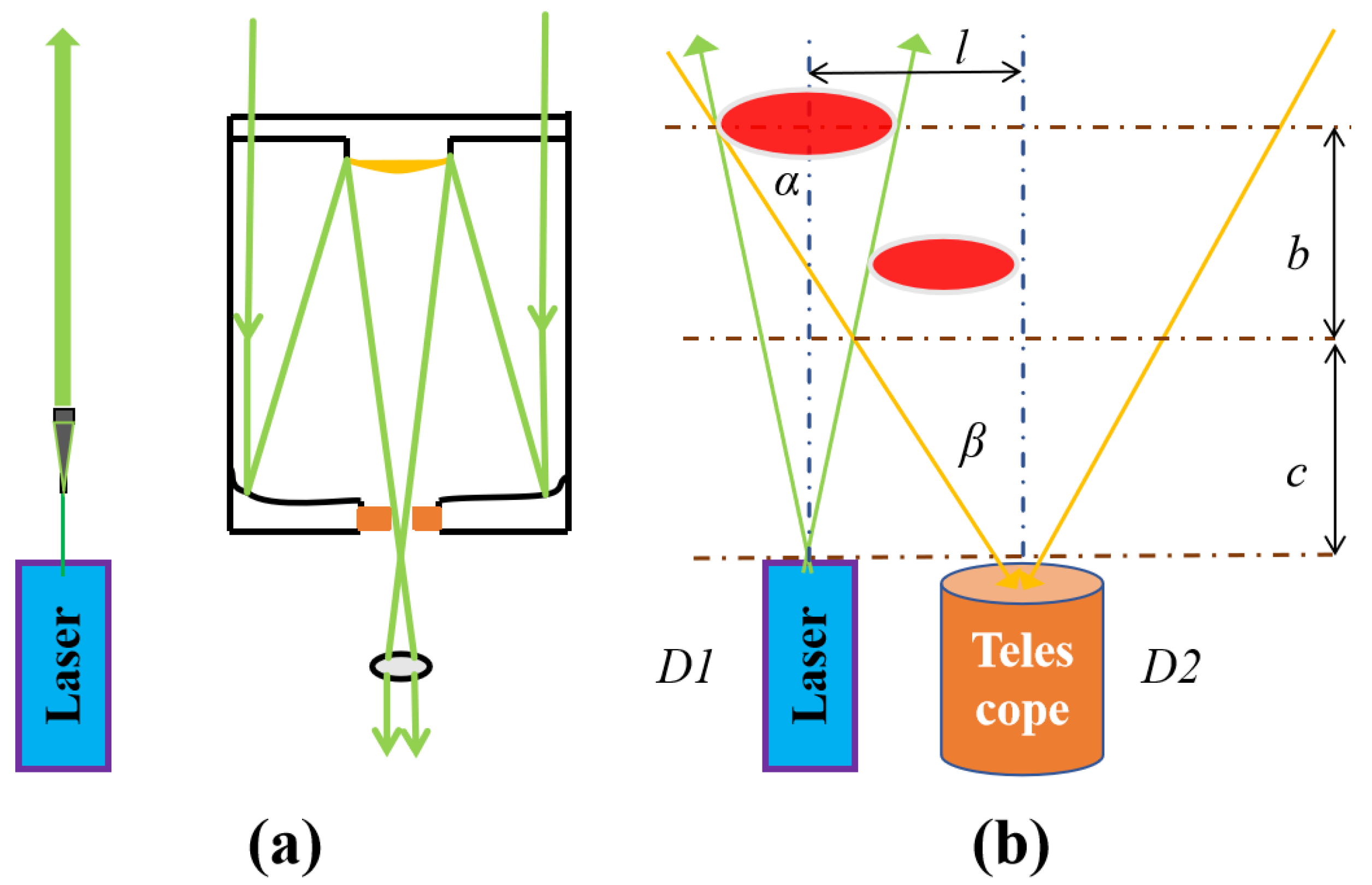
2.1. Lidar System Optical Path

The optical path of the transceiver subsystem in most Lidar systems is categorized into coaxial and non-coaxial configurations. Using the non-coaxial Lidar system as an example, during detection, the region receiving the atmospheric echo signal can be divided into three distinct sections. As shown in Figure 1a, the emitted beam is parallel to the optical axis of the receiving telescope. D1 and D2 represent the beam diameter and telescope aperture, respectively. At distance c, the beam begins to enter the telescope’s receiving field of view, marking this area as the blind zone. At distance b, only a few beams can enter the receiving field of view, thus this region is called the transition zone. Beyond distance b, the beam can fully enter the receiving field of view, and this region is referred to as the full zone. This indicates that during the detection process, the reception of the atmospheric echo signal varies across different regions. Therefore, selecting a more suitable self-alignment adjustment method is crucial.

2.2. Traditional Optical Alignment Method

Currently, two common methods for Lidar optical alignment are used [16,17]. The first method is the echo signal strength method, and the second is the automatic spot collimation method. The echo signal intensity method involves scanning the emitted laser in a specific direction within the atmosphere. The optical axis parallelism of the transceiver system is determined by observing the intensity of the atmospheric echo signal at a predetermined height. The direction with the strongest signal strength is considered the approximately parallel direction of the optical axis. During collimation correction, scanning in different directions within the atmosphere is necessary to obtain the trapezoidal curve depicting the relationship between the back-scattered signal and scanning angle. When the echo signal is at the center of the trapezoidal curve, optical axis parallelism is optimized. The automatic spot collimation method uses optical imaging devices to achieve self-alignment by adjusting the spot quality of the back-scattered signal on the detector. The most commonly used approach involves feeding back the spot position of the back-scattered signal on the CCD target surface to the calculation program. Subsequently, based on the preset spot position, the optical device at the transmitting end is adjusted using the stepper motor, thereby optimizing the optical axis parallelism of the transceiver system.

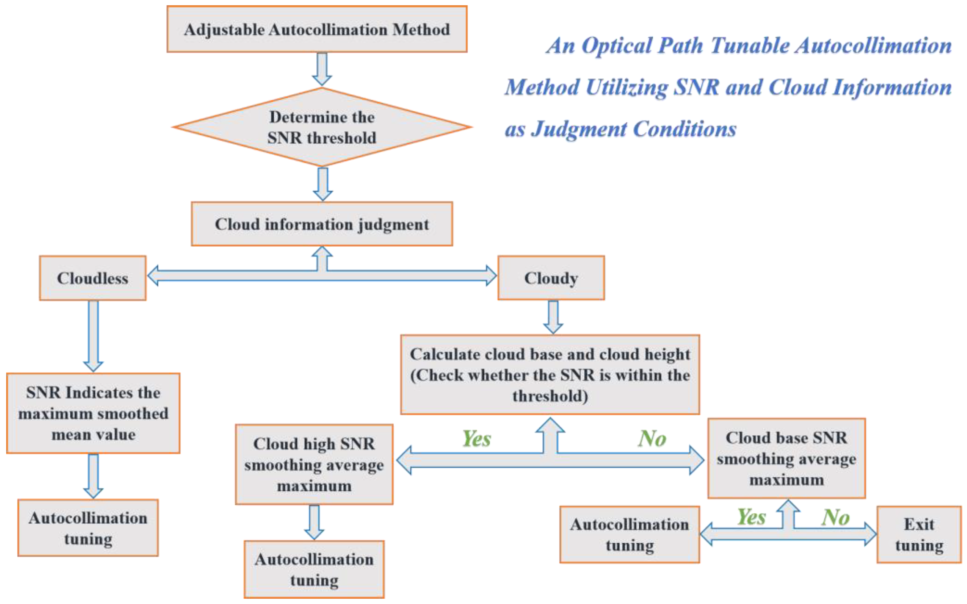
2.3. Adjustable Optical Alignment Method

In most previous Lidar detection experiments, the optical alignment process assumes a uniform atmospheric distribution, disregarding variations in cloud information and aerosol concentrations. Atmospheric parameters, such as the backscattering coefficient and extinction coefficient, are assumed to be constant. However, in practical scenarios, especially in the complex climate of eastern China, the spatial distribution of atmospheric parameters is non-uniform and exhibits temporal variability. This phenomenon has been confirmed by numerous studies, including those conducted by this research group. Additionally, wind Lidar and scanning transmittance Lidar systems, which rely on rotational detection, cannot maintain consistent atmospheric states across all radials, necessitating the use of judgment algorithms for precise optical alignment under varying weather conditions. The SNR of the Lidar measurement signal is not only an important indicator for evaluating the system’s detection performance but also a key parameter for assessing the collimation effect. As the backscattering signal from a cloud is very large, visible peaks appear in SNR traces (as shown in Figure 2). Accordingly, the system’s actual line-of-sight direction is used to set an appropriate SNR as the criterion for signal strength, and the influence of cloud conditions on the optical alignment system is divided into two aspects.

By setting a threshold value and applying the slope method, the cloud position can be initially determined, along with the height information of both the cloud base and cloud top. The strong scattering and absorption of the laser by the cloud significantly attenuates pulse energy, weakening the signal strength above the cloud and reducing the SNR. Therefore, an indicator must be selected based on different situations, with the judgment logic of the adjustable optical alignment method illustrated in Figure 3. Specifically, the signal can be categorized into four types based on the signal score: no cloud, clouds with sufficient SNR, clouds with insufficient SNR but adequate SNR at the cloud base, and clouds with insufficient SNR overall. Different optical alignment strategies are employed for each of these four cases. An area with an SNR between 5 and 10, at a height of more than 20 km, can be selected as the evaluation range. The SNR curve for this region is smoothed, and the average SNR is used as the criterion. The optical alignment process is complete when the average value reaches its highest point. If clouds are detected based on the SNR, with the SNR ranging from 5 to 10 and the height still around 20 km, the cloud is considered to have minimal impact on the SNR curve, allowing the previous optical alignment steps to be repeated. If only the SNR at the cloud base meets the 5 to 10 range, while the SNR above the cloud is insufficient, the SNR from the cloud base to 2–3 km below should be selected for smoothing, with the average value used as the criterion. If the SNR at the cloud base and above does not meet the required conditions, it is deemed that the atmospheric conditions are unsuitable for atmospheric detection. The system will then exit the optical alignment process and provide appropriate notifications.

3. Experiment

3.1. RRDWL System Overview

RRDWL is a wind Lidar system developed by our research group for three-dimensional detection of wind fields in the middle and upper atmosphere. It supports full rotational detection and has demonstrated favorable detection capabilities [23,24]. The overall structure of RRDWL is depicted in Figure 4. To enable single-point detection of the three-dimensional atmospheric wind field, the system is housed in equipment measuring 5 m in length, 2.7 m in width, and 2.4 m in height, weighing approximately 6 tons, and placed on a circular rotating platform with a 6-m diameter. The equipment is designed for comprehensive observation, with the roof featuring a rectangular skylight that allows the telescope to tilt up to 45° toward the zenith, thereby covering a broader observational range. The rotating table has a maximum speed of 6°/s and can rotate within a 0° to 540° range. Meanwhile, the main technical parameters of RRDWL are listed in

Table 1. Lidar system parameters.

Measurement Performance
Height resolution	0.275–1.1 km (changeable)
Time resolution	30 min (changeable)
Laser wavelength	532.1 nm
Pulse energy	350 mJ
Repetition rate	30 Hz
Spectral bandwidth (FWHM)	70 MHz
Divergence angle	50 μrad
Telescope diameter	800 mm
FOV	100 μrad
IF bandwidth (FWHM)	0.3 nm
Beam divergence	2.5 mrad
Transient recorder	12 bit, 20 MHz sampling rate
Acquisition card	12 bit, 1 GHz sampling rate

.

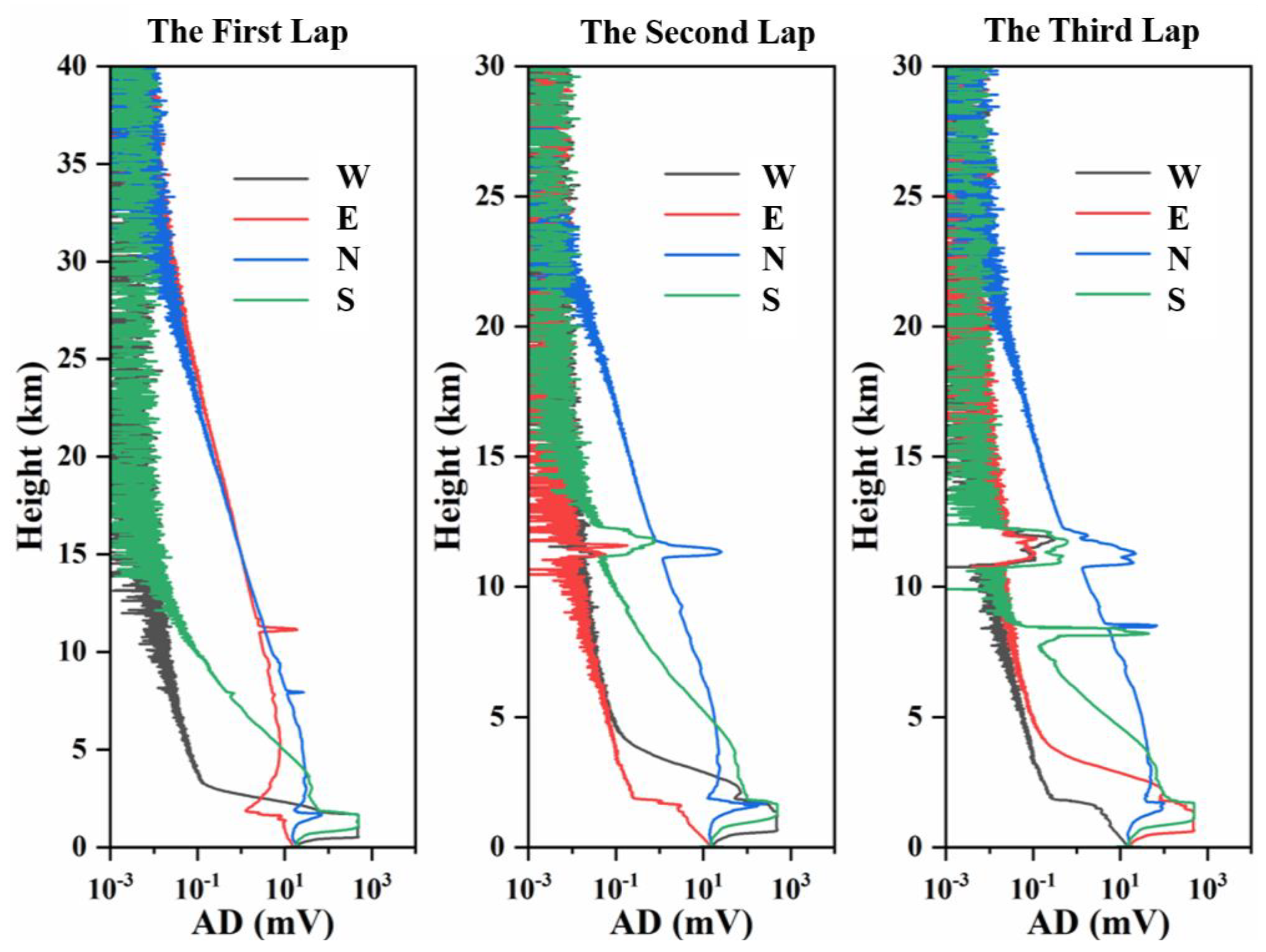
3.2. RRDWL Optical Path Imbalance

A recent study highlights that the complex working environment of the observation site imposes significant constraints, challenging the system’s ability to maintain continuous detection [25]. As a result, the RRDWL is unable to provide reliable long-term atmospheric wind field data. Due to the use of a single unit for integral rotation (weighing nearly 6 tons), the stability of the transceiver system is inevitably affected by vibrations and structural deformations during detection, which may significantly impact performance. Therefore, the main components of the RRDWL are treated as point masses for simplicity. The system’s mechanical analysis under working conditions is performed using the finite element method. As the load varies with time during operation, stress, strain, and displacement also fluctuate accordingly. By investigating modal deformation and corresponding frequencies, we can identify structural components with low rigidity and high susceptibility to excitation. Boundary conditions are applied to constrain the inner surface of the chassis shaft, and rotational conditions are incorporated to simulate the system’s operating state during the detection experiment. As shown in Figure 5, the displacement and shape variables of the system structure are presented for a velocity condition of 2°/s. It is evident that the deformation caused by the centrifugal force in the equipment shelter is minimal due to the low rotational speed. In contrast, the rotating platforms experience more significant deformation. It can be inferred that RRDWL is highly susceptible to low-frequency vibrations from chassis rotation during detection experiments, as well as vibrations induced by road fluctuations during transport.

Combined with Figure 4 and Figure 5, it can be seen that the deformed part of the chassis is located near the launch subsystem. Signal misalignment was observed during the detection experiment, further confirming the previous simulation results. Figure 6 illustrates that on the evening of 13 March 2022, the system performed a continuous detection test. Before the wind field detection experiment, a pre-test was conducted to observe the signal-to-noise ratio under cloudy conditions; therefore, no gated signals were used. After the experiment, three sets of line-of-sight atmospheric echo signals were collected following three rotations. In a relatively short period (approximately 90 min), the atmospheric echo signal in each direction showed significant deviation. To determine whether the SNR changed significantly due to high clouds, a comparison of atmospheric echo signals for three consecutive rotations in the north, east, south, and west directions was created, as shown in Figure 7. The results show that the atmospheric echo signal in different line-of-sight directions indeed exhibits significant deviation, with an uneven variation pattern. Therefore, it is inferred that this is due to the uneven ground and the deformation of the shelter caused by rotation, which disrupts the collimation of the optical path in the transceiver subsystem.

3.3. RRDWL Optical Alignment Test

To prevent additional optical path errors during spot detection in the transmitting optical path, a tunable optical alignment system is designed by integrating the original optical path of the transmitting subsystem with the echo signal intensity method. First, a high-precision two-dimensional electric adjustment frame is placed between the laser beam expander and the telescope. To improve long-term stability and provide enhanced shock protection, cemented carbide pads, thickened front and rear panels, and optimized rigid springs are used to support high-precision mirrors with a diameter of up to 4 inches. During the optical alignment correction of the transmitted beam, the high-precision piezoelectric 2-D mirror adjustment frame is driven by a stepper motor to perform scans in the north-south and east-west directions, respectively. This process consists of two steps: rough scanning and fine scanning. With the exception of the initial line-of-sight direction, which remains stationary, detecting the other three directions requires rotating the system. However, ground unevenness during rotation or other environmental factors can cause a significant shift in the optical axis, potentially leading the laser beam to exit the telescope’s receiving field of view entirely. In the initial stage of optical alignment, the stepper motor controls the high-precision piezoelectric two-dimensional reflector adjustment frame to perform a rapid spiral sweep with a relatively large step size. By analyzing the characteristics of the atmospheric echo signal (noise or signal), we can determine whether the laser beam is within the telescope’s field of view. Notably, the adjustment angle must be precisely defined to avoid excessive step size, which could cause the laser beam to deviate from the telescope’s receiving field of view. The specific details are outlined below:

$$H\theta \le {2(\mathrm{D}}_L{+\mathrm{D}}_T)$$

$${\mathrm{D}}_L{=(\mathrm{S}}_L+H{\theta }_{DIV})/2,$$

$${\mathrm{D}}_T{=(\mathrm{S}}_T+H{\theta }_{FOV})/2,$$

$$\theta \le {\theta }_{DIV}+{\theta }_{FOV},$$

where $H$ represents the reference height, ${\mathrm{D}}_L$ is the beam radius at $H$, ${\mathrm{D}}_T$ is the receiving radius at $H$, ${\theta }_{DIV},{\theta }_{FOV}$ are the beam divergence angle and the receiving field of view angle, respectively.

Once the beam is collimated into the receiving field of view, the coarse sweep cannot precisely adjust the signal intensity to the optimum level. Therefore, a fine cross-type sweep is required, with the stepper motor’s step size reduced, as shown in Figure 8. Initially, the position A of the beam in the receiving field of view after rough scanning is used as the starting point. The step size is reduced, and scanning continues until the beam exits the receiving field of view, which is marked as point B. The midpoint between point A and point B is defined as point C, which serves as the starting point for the subsequent scan. Point C is assumed to be the location where the atmospheric echo light signal is strongest in the direction of AB. Scanning then continues in a direction perpendicular to AB. Due to the small sweep step size and the extended time required, 1–2 steps on both sides of point C are taken when approaching it to assess the signal strength, thus improving self-alignment efficiency. The scan proceeds in the direction of the weakened signal until the laser beam exits the receiving field of view again, marked as point D. The scan continues in the reverse direction until the laser beam exits the receiving field of view again, labeled as point E. The midpoint between point D and point E is defined as point O, which represents the optimal position for the atmospheric echo signal strength. Point C and point O are not directly determined during the scanning process but must be identified through an algorithm. Ideally, only the effects of emitted laser energy jitter and the average aperture effect of the receiving telescope are considered. The adjustment angle between the atmospheric echo light signal and the optical axis at the reference height can be modeled as a trapezoidal function. Considering background noise, detector noise, and laser jitter, the position of point O is:

$$W={\displaystyle \frac{\sum P_i{W}_i}{\sum P_i}}$$

where $W$ represents the O point position, $W_i$ is the stepper motor position, and $P_i$ is the signal strength.

The adjustable optical alignment system performs collimation adjustment in three main steps:

(1)

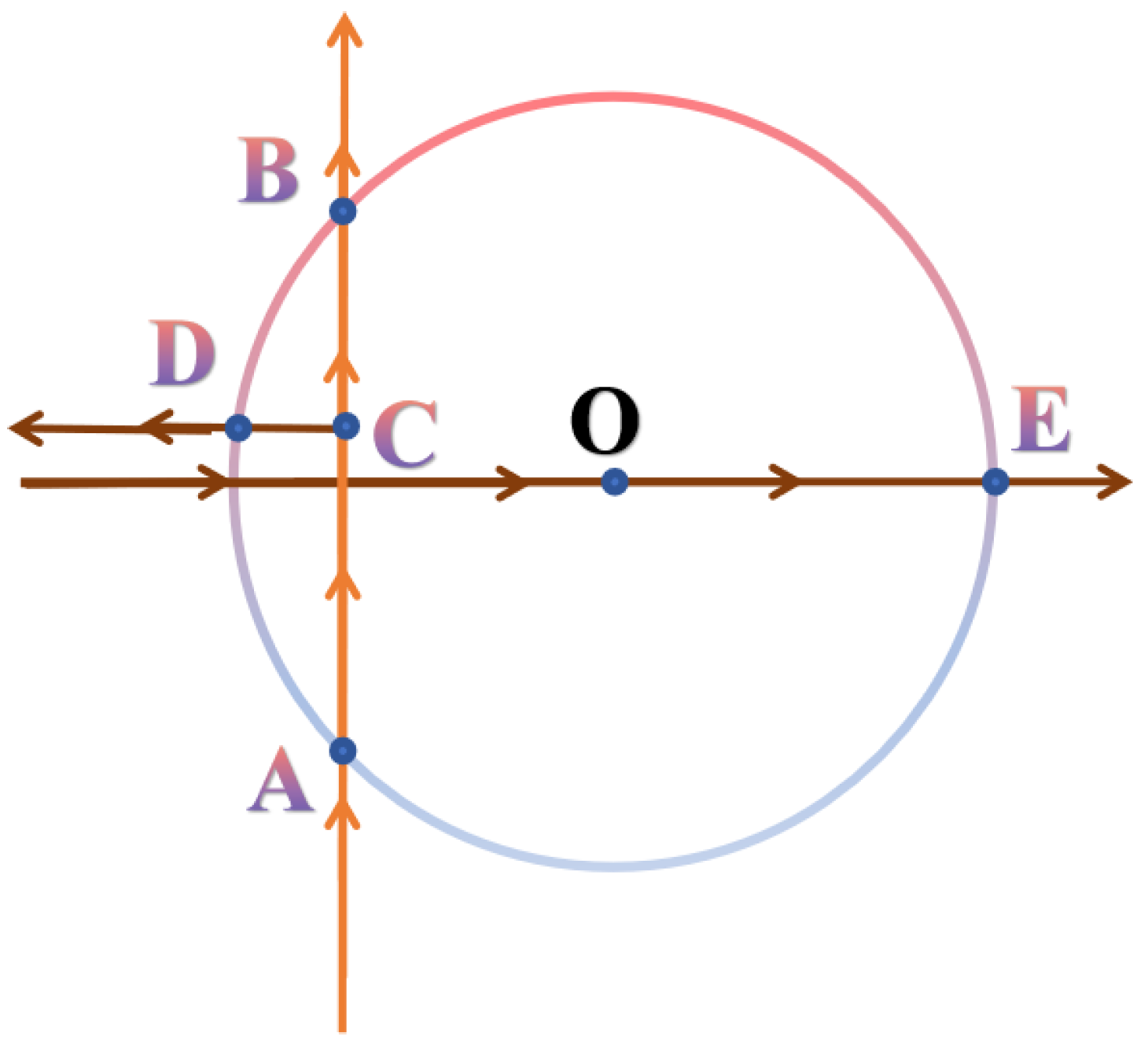
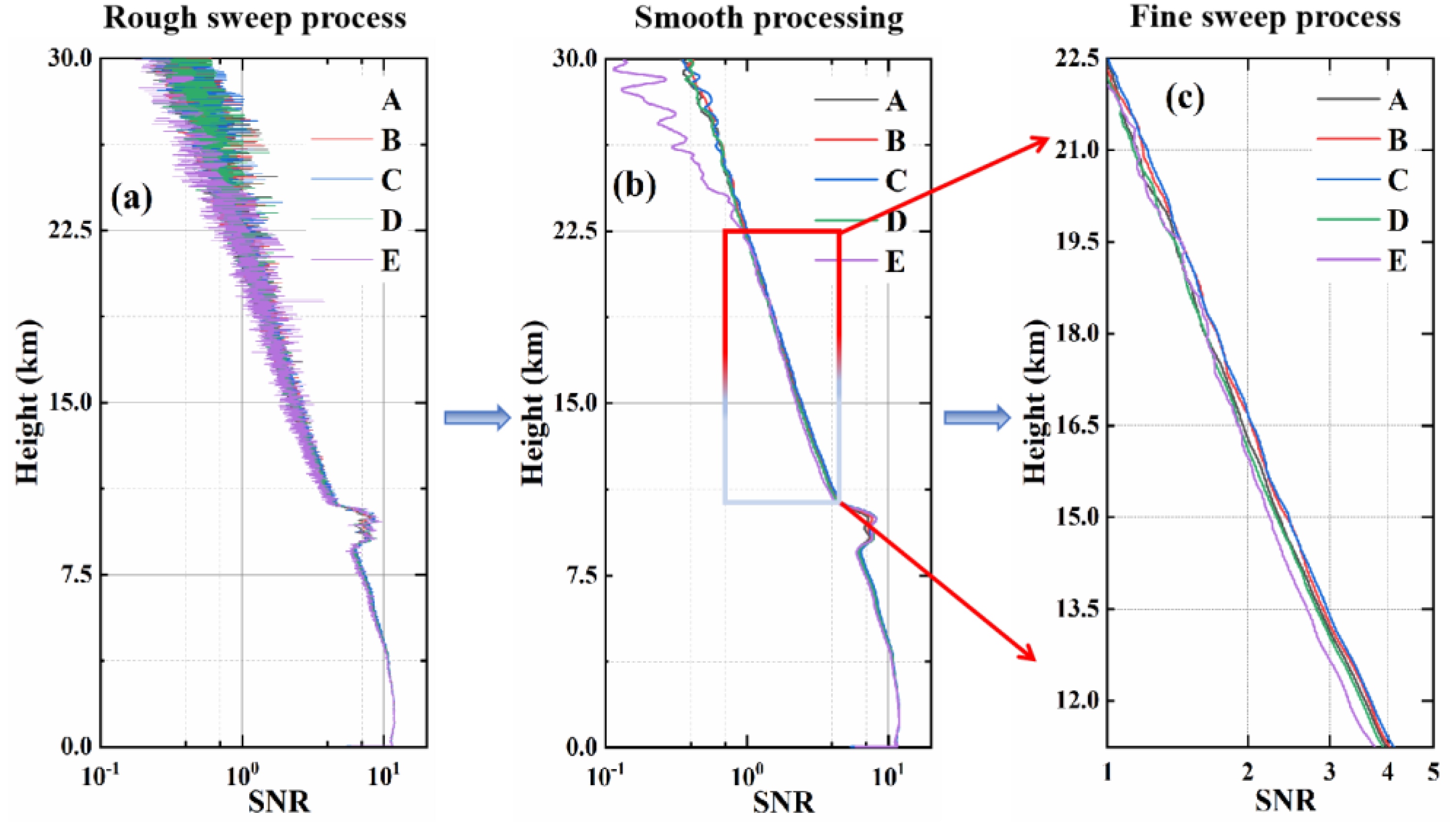
First, if atmospheric echo signal misalignment occurs in the direction of the four lines of sight after one full rotation of the rotating platform, broad-spectrum dimming (coarse adjustment) should be performed. The adjustment step for the high-precision two-dimensional electric adjustment frame is set to 300, and the initial adjustment position is designated as S₀. Moving 300 steps in a specified direction yields data S₁. If S₀ < S₁, 300 steps are moved in the opposite direction, and the resulting data are S₂. If S₀ < S₂, return to position S₀.

(2)

Second, after completing the coarse adjustment, the optical axis position at this stage is recognized as being within the field of view of the receiving telescope. The optimal position after the coarse adjustment is adopted as the initial position, and four datasets are acquired in both left and right directions, each with a step length of 100, for the second rough adjustment to determine the position S₃ of the most favorable group.

(3)

Finally, fine adjustment is performed at the position identified by S₃ as the primary collimation of the optical axis. Four datasets are obtained from both left and right directions, each with a step length of 20, for fine adjustment, yielding position S₄ as the optimal position. Ultimately, S₄ represents the most suitable collimation position.

Additionally, the optical alignment adjustment process occurs only before the start of each line-of-sight detection experiment. Optical alignment adjustment is not conducted simultaneously with the detection experiment. This implies that RRDWL requires only four optical alignment adjustments for each wind field detection experiment. This significantly enhances detection efficiency and effectively mitigates the influence of atmospheric conditions on the measurement results over time.

4. Results

4.1. RRDWL Optical Alignment Results

A significant optical alignment calibration test was conducted on 12 June 2022, at Hefei Science Island, China, as shown in Figure 9. The experimental process involved a set of optical alignment tests, during which a total of 300 laser pulses were emitted. The collimation sequence followed a specific pattern: E → D → A → C → B → C, as shown in Figure 9a. A specific criterion was used to designate the effective detection height area based on the SNR. Areas with an SNR exceeding 1 were defined as effective detection zones. Through careful observation and analysis of the experimental images, the effective height was determined to be approximately 22.5 km under the given conditions. After determining the effective height region, the SNR profile was smoothed to obtain more accurate experimental data, as shown in Figure 9b. Based on this, the average SNR within the judgment region was calculated and processed. Figure 9c shows a magnified profile of the judgment area to provide a clearer visualization of the SNR details. After magnification, the SNR at this position showed a specific order: C > B > A > D > E. Based on the above order of the signal-to-noise ratio, the operational procedure for optical alignment regulation was established. Initially, the SNR corresponding to profile E was set as the starting position, and fine-tuning operations were performed in the X direction to obtain profile D. Next, the SNR of the judgment region was compared. If the SNR of the judgment region at D was greater than at E, the fine-tuning steps were repeated according to the established adjustment procedure, continuing in the X direction until profile B was obtained. At this point, the SNR of the judgment region was rechecked, revealing that profile B was smaller than profile C. Based on this result, a callback operation was performed in the opposite direction of X to reacquire image C. Once the adjustment operation in the X direction was completed and the corresponding image was determined, the same series of steps were repeated in the Y direction. The profile with the highest SNR within the judgment area was identified through continuous adjustment and comparison. At this stage, the optical alignment process was considered complete.

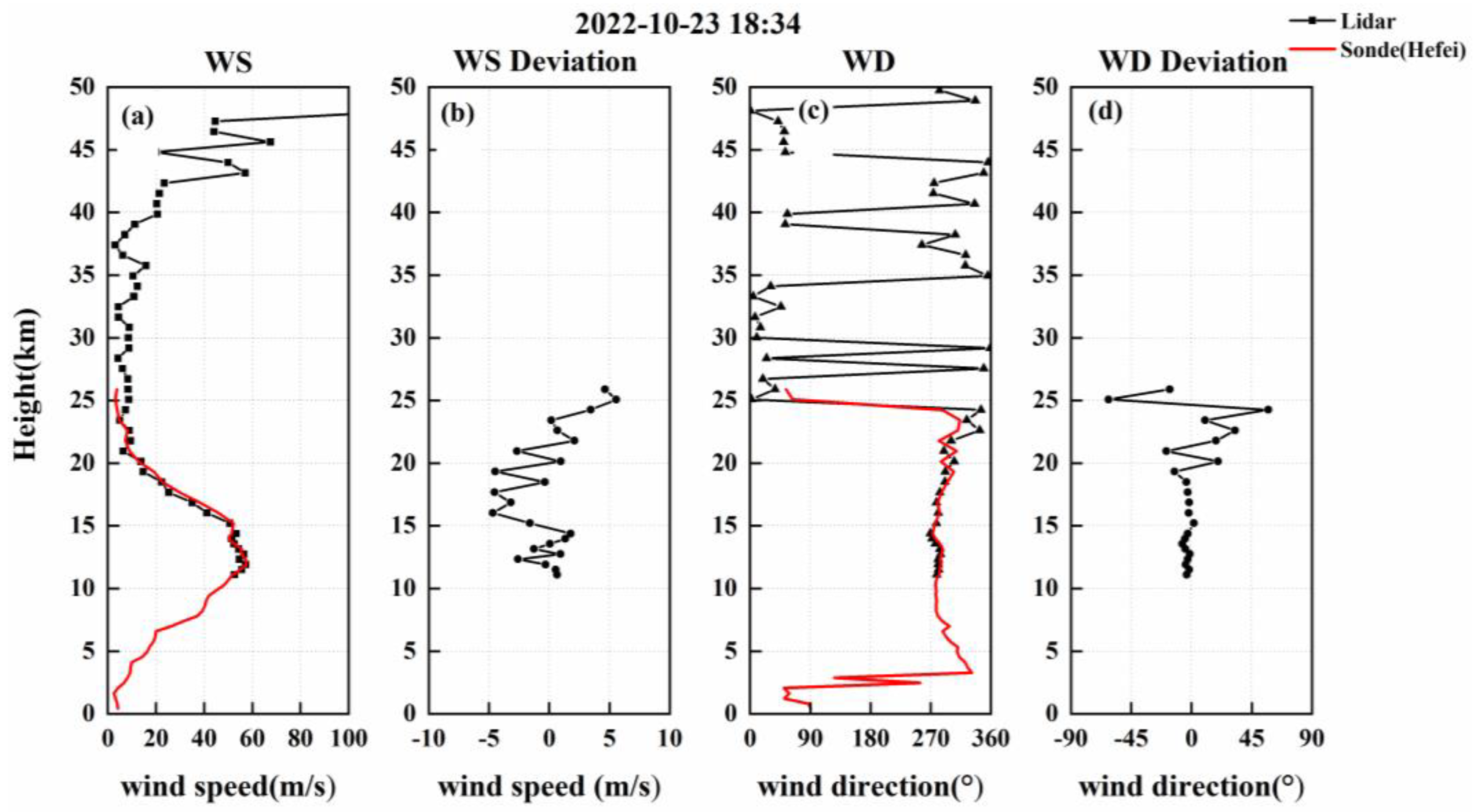
4.2. Atmospheric Horizontal Wind Field Results

Previous studies by the research group have shown that the RRDWL can detect atmospheric wind fields at altitudes between 38 and 42 km in an external environment after its development [23,25]. However, the random error in the four-line wind profile at 36 km is approximately 10 m/s, and the random error in horizontal wind speed is about 11.3 m/s. This indicates that factors like optical axis alignment, vibration control, ambient temperature stability, and FPI parallelism imbalance significantly influence the SNR of RRDWL, thereby increasing wind speed uncertainty. To compare the detection height and measurement accuracy of the RRDWL before and after optical alignment calibration, a set of experiments was conducted at the same site (Science Island, Hefei, China) on the night of 23 October 2022. In this experiment, the RRDWL fired 8000 laser pulses for each line of sight. The addition of the adjustable optical alignment system extended the experiment time from 24 to 32 min. To improve the system’s SNR, spatial averaging of the raw data was performed, achieving a distance resolution of 300 m. Simultaneously, the signal gate opening time delay after laser pulse Q-modulation was set to 80 μs. This allows the RRDWL to effectively receive the echo signal from a distance of 10 km, helping to avoid detector saturation caused by strong low-altitude scattered signals. A weather balloon with a radiosonde was released at the same location and reached an altitude of 25.21 km within 120 min, covering the RRDWL’s operating time.

Figure 10 shows the horizontal wind speed profile, wind direction profile, and absolute deviation between the RRDWL and Sonde. The horizontal wind speed and wind direction of the RRDWL and Sonde show almost identical trends within the comparable height range (10–25 km). As shown in Figure 10b, except for a thin layer near 25 km, the absolute deviation is about 6.2 m/s, while the deviation in other height ranges is within 5 m/s. Above 14 km, the absolute deviation increases significantly as wind speed decreases. At 11.92 km, near the tropopause, the horizontal wind speed reaches a maximum of 57.21 m/s. The wind speed gradually decreased to within 6 m/s at an altitude of 20.9 km. In the range of 21–25 km, a weak wind layer appeared, with peak winds around 8.65 m/s. Additionally, as shown in Figure 10c, westerly winds (279° to 344°) dominate the 10 km to 25 km range. Both devices detected wind shear at an altitude of approximately 25.1 km. Conversely, Figure 10d shows that the wind direction deviation between the two devices is less than 3° below 19 km. Between 19 km and 23 km, the wind direction deviation is less than 10°. However, above 23 km, the RRDWL wind direction profiles showed significant oscillations. In summary, the RRDWL and Sonde measurements agree well in both wind speed and direction from 11 km to 25 km. However, differences exist in the thin layer at higher altitudes, likely due to differing instrument principles, measurement errors, or environmental conditions.

4.3. RRDWL Performance Optimization Evaluation

To evaluate the detection height and accuracy of the RRDWL after optical alignment optimization, the wind field results from 23 October 2022 were analyzed for errors. As shown in Figure 11, the SNR profiles for four line-of-sight directions were analyzed. At an altitude of 30 km, the measured SNR was approximately 454, about four times higher than the 112 before optical alignment optimization. At 42 km, the measured SNR was about 44.6, approximately four times higher than the 10 prior to optical alignment optimization. Furthermore, the detection height for an SNR of approximately 10 was about 49 km, 1.2 times higher than the effective detection height of 42 km before optical alignment optimization. Moreover, after optical alignment optimization, the SNR jitter in the four line-of-sight directions beyond 30 km was minimal, indicating that the signal was stable. It can be inferred that the primary factor causing SNR inconsistency at the same height in different line-of-sight directions was the uneven atmospheric distribution, with the impact of system hardware on signal strength and noise level being negligible. This also demonstrates that the tunable optical alignment system effectively ensured beam quality and optical path collimation during detection.

To assess the long-term detection performance of RRDWL after optical alignment optimization, 8000 pulses with an SNR of 10 were used as the evaluation criteria. A statistical analysis was performed on the signals acquired during the continuous wind field detection experiment. The statistical results are shown in Figure 12, with Figure 12a illustrating the effective detection heights of the two edge channels, and Figure 12b depicting the combined effective detection heights. As shown in Figure 12a, in edge channel 1, there are 6 datasets with effective heights below 48 km, 58 datasets between 48 km and 50 km, and 36 datasets above 50 km. In contrast, for edge channel 2, there are 4 datasets with effective altitudes below 48 km, 59 datasets between 48 km and 50 km, and 37 datasets above 50 km. Figure 12b shows 4 datasets below 48 km, 59 datasets between 48 km and 50 km, and 37 datasets above 50 km. In summary, after optimizing optical alignment performance, the effective detection height of RRDWL is primarily concentrated between 48 km and 51 km. Compared to the 38 km to 43 km range, the effective detection altitude has increased by approximately 1.2 times.

The random error calculated from the SNR reflects the uncertainty in wind speed measurements and can be used to assess their accuracy. Therefore, the random error of the horizontal wind profile was computed, as shown in Figure 13. The results in the figure show that the random error of the horizontal wind profile increases exponentially with height. At an altitude of 39 km, the random error of the horizontal wind speed was approximately 10 m/s.

A comparison of the horizontal wind profiles obtained by RRDWL and Sonde is shown in Figure 14. The horizontal wind profile trends obtained by both devices are nearly identical.

The measured absolute deviation of wind speed is compared with the random error calculated from the SNR. As shown in Figure 15, except for a thin layer around 25 km, the absolute deviation of wind speed stays below 5 m/s and is nearly zero at several altitudes. Similarly, in the comparison height range, the change trends of the two devices are nearly identical. Based on these findings, it can be concluded that the RRDWL with optimized optical alignment performance has significantly improved wind speed measurement accuracy. In the comparable altitude range of 10 to 30 km, the wind speed error is less than 5 m/s, indicating that the horizontal wind field results obtained by RRDWL are more accurate and reliable.

A statistical analysis was conducted on 100 datasets obtained during the continuous detection experiment to enhance the representativeness of the results. Since the sonde’s detection height is generally below 30 km, the random error sequence of the horizontal wind speed at 30 km, obtained from RRDWL, was computed and is shown in Figure 16. The statistical analysis shows that, out of the 100 datasets, the random error in horizontal wind speed was less than 3 m/s in 2 sets, greater than 5 m/s in 10 sets, and between 3 m/s and 5 m/s in the remaining 88 sets, with an average error of approximately 4.4 m/s. Additionally, the figure shows some jitter in adjacent datasets, indicating a disparity in the horizontal wind speed error across the different experimental groups. This disparity may result from a combination of horizontal atmospheric inhomogeneity and systematic errors. However, the jitter is within 3 m/s, which confirms the reliability of the horizontal wind field data obtained by RRDWL.

Finally, Figure 17 presents the absolute deviation of wind speed between RRDWL and Sonde within the comparable altitude range (10 km to 30 km), before and after optical alignment optimization. The overall trend of the absolute deviation of wind speed, both before and after optimization, is similar, and it increases with altitude between 16 km and 30 km. However, some disparities exist. Specifically, the maximum absolute deviation of wind speed in RRDWL after optimization does not exceed 8 m/s, while the maximum deviation before optimization approaches 15 m/s. Additionally, in the 10 km to 16 km range, the absolute deviation of RRDWL wind speed after optimization does not exceed 5 m/s, with a minimum value of approximately 1 m/s, while the deviation before optimization is around 6 m/s. In summary, the overall absolute deviation of wind speed in RRDWL improves after adjustable optical alignment optimization. Within the comparable altitude range, RRDWL provides higher wind speed measurement accuracy, with a smaller maximum deviation. The deviation is also significantly reduced at lower altitudes, further confirming the reliability of the adjustable optical alignment method.

5. Discussion

Previous studies by this group have identified the key factors influencing the detection performance of RRDWL, which include the following:

(1)

Laser frequency stability. In RRDWL operations, seed injection lasers are commonly used. However, these lasers are highly sensitive to external factors such as temperature fluctuations and vibrations, which can cause frequency drift. This instability may introduce significant errors in subsequent wind speed inversion, severely affecting the accuracy of wind speed measurements and analysis;

(2)

Divergence angle and stability of the laser beam. During detection, the emitted laser beam may jitter or exhibit an amplification effect. This phenomenon hampers the accurate identification of Doppler frequency shifts caused by wind, which in turn increases the errors in wind speed inversion and hinders the accurate acquisition of wind speed data;

(3)

Instrument stability and calibration issues. The direct detection wind Lidar system often consists of multiple high-precision instruments. In real-world conditions, environmental factors such as temperature changes and vibrations can induce system errors in these instruments. Furthermore, the stability of the instruments and calibration processes may negatively impact the overall detection performance;

(4)

Complex atmospheric conditions. Most direct detection wind Lidar systems are currently deployed in high-latitude regions or areas with favorable meteorological conditions. However, atmospheric conditions in central and eastern China, as well as low-latitude areas, are highly complex, with significant spatiotemporal inhomogeneity. In such an environment, factors like clouds, aerosols, and turbulence are intertwined, directly affecting wind Lidar performance and interfering with the accuracy of detection results.

As previously discussed, the RRDWL weighs approximately 6 tons and requires a full rotation during detection experiments. The uneven ground conditions and the system’s irregular mass distribution can directly and significantly affect the collimation of both the receiving and emitting paths. Furthermore, the RRDWL is designed primarily for detecting mid-to-upper atmospheric wind fields over eastern China. In practical atmospheric wind field detection, the influence of strong scattered signals from clouds, aerosols, and other particles on Lidar echo signals is significant. These scattered signals can substantially interfere with the characteristics and quality of echo signals, thereby affecting subsequent detection and analysis. Specifically, it is important to highlight that the direct detection wind Lidar using an F-P interferometer as a frequency identifier relies on changes in the intensity of the echo signal to measure the wind field. The Doppler shift induced by wind can be accurately detected only by resolving changes in the transmittance spectral lines, thus enabling precise wind field measurements. This mechanism imposes strict SNR requirements on the RRDWL. Only with a high SNR can the system operate stably and accurately, ensuring the reliable acquisition of wind field data. The optical alignment test results and the wind field detection experiments above demonstrate that the proposed adjustable optical alignment method offers significant advantages. Specific data show that this method improves SNR by nearly four orders of magnitude, resulting in a corresponding improvement in wind field measurement accuracy by the same factor.

6. Conclusions

In conclusion, this study introduces a novel tunable optical alignment approach designed to improve the optical path stability of RRDWL systems, particularly in complex environmental conditions. By utilizing cloud data and SNR intensity, the proposed method significantly enhances traditional echo signal strength methods. The stratified optical alignment strategy, which is based on the SNR at the cloud base and height, enables precise wind field detection in the middle and upper atmosphere. Experimental results show a significant enhancement in the detection capabilities of the optimized RRDWL system. Specifically, the maximum effective detection height of the RRDWL has increased to 51 km, representing a 21% increase from the previous 42 km. The random error in horizontal wind speed at 30 km altitude has been reduced to 4.4 m/s, approximately 61% lower than the previous 11.3 m/s. The minimum measurement deviation is now only 1 m/s. These results highlight the effectiveness and reliability of the proposed tunable optical alignment method in improving the performance of Lidar systems under diverse meteorological conditions and complex operational scenarios.

References

1. Liu, Z.; Barlow, J.F.; Chan, P.-W.; Fung, J.C.H.; Li, Y.; Ren, C.; Mak, H.W.L.; Ng, E. A Review of Progress and Applications of Pulsed Doppler Wind LiDARs. Remote Sens. 2019, 11, 2522. [Google Scholar] [CrossRef]
2. Jinlong, Y.; Haiyun, X.; Tianwen, W.; Lu, W.; Bin, Y.; Yunbin, W. Identifying cloud, precipitation, windshear, and turbulence by deep analysis of the power spectrum of coherent Doppler wind lidar. Opt. Express 2020, 28, 37406–37418. [Google Scholar]
3. Wang, Z.; Liu, Z.; Liu, L.; Wu, S.; Liu, B.; Li, Z.; Chu, X. Iodine-filter-based mobile Doppler Lidar to make continuous and full-azimuth-scanned wind measurements: Data acquisition and analysis system, data retrieval methods, and error analysis. Appl. Opt. 2010, 49, 6960–6978. [Google Scholar] [CrossRef] [PubMed]
4. Xu, H.; Li, J. Performance analysis of dual-frequency lidar in the detection of the complex wind field. Opt. Express 2021, 29, 23524–23539. [Google Scholar] [CrossRef] [PubMed]
5. Dou, X.; Han, Y.; Sun, D.; Xia, H.; Shu, Z.; Zhao, R.; Shangguan, M.; Guo, J. Mobile Rayleigh Doppler Lidar for wind and temperature measurements in the stratosphere and lower mesosphere. Opt. Express 2014, 22, A1203–A1221. [Google Scholar] [CrossRef]
6. Hao, R.; Dou, X.; Xue, X.; Sun, D.; Han, Y.; Chen, C.; Zheng, J.; Li, Z.; Zhou, A.; Han, Y.; et al. Stratosphere and lower mesosphere wind observation and gravity wave activities of the wind field in China using a mobile Rayleigh Doppler Lidar. J. Geophys. Res. Space Phys. 2017, 122, 8847–8857. [Google Scholar]
7. Wu, S.; Liu, B.; Liu, J.; Zhai, X.; Feng, C.; Wang, G.; Zhang, H.; Yin, J.; Wang, X.; Li, R.; et al. Wind turbine wake visualization and characteristics analysis by Doppler lidar. Opt. Express 2016, 24, A762–A780. [Google Scholar] [CrossRef]
8. Liu, Q.; Zhu, W.; Jin, X.; Qing, C. Real-Time Synchronous Acquisition and Processing of Signal in Coherent Doppler Wind Lidar Using FPGA. Remote Sens. 2023, 15, 5673. [Google Scholar] [CrossRef]
9. Yu, C.; Shangguan, M.; Xia, H.; Zhang, J.; Dou, X.; Pan, J.W. Fully integrated free-running InGaAs/InP single-photon detector for accurate lidar applications. Opt. Express. 2017, 25, 14611–14620. [Google Scholar] [CrossRef]
10. Li, Q.; Zhang, X.; Feng, Z.; Chen, J.; Zhou, X.; Luo, J.; Sun, J.; Zhao, Y. Enhanced Wind-Field Detection Using an Adaptive Noise-Reduction Peak-Retrieval (ANRPR) Algorithm for Coherent Doppler Lidar. Atmosphere 2024, 15, 7. [Google Scholar] [CrossRef]
11. Ma, B.; Zong, Y.; Li, Z.; Li, Q.; Zhang, D.; Li, Y. Status and prospect of opto-mechanical integration analysis of micro-vibration in aerospace optical cameras. Opt. Precis. Eng. 2023, 31, 822–838. [Google Scholar] [CrossRef]
12. Tavakolibasti, M.; Meszmer, P.; Böttger, G.; Kettelgerdes, M.; Elger, G.; Erdogan, H.; Seshaditya, A.; Wunderle, B. Thermamechanical-optical coupling within a digital twin development for automotive LiDAR. Microelectron. Reliab. 2023, 141, 114871. [Google Scholar] [CrossRef]
13. Philip Stahl, H.; Kuan, G.; Arnold, W.R.; Brooks, T.; Brent Knight, J.; Martin, S. Habitable-Zone Exoplanet Observatory baseline 4-m telescope: Systems-engineering design process and predicted structural thermal optical performance. J. Astron. Telesc. Instrum. Syst. 2020, 6, 034004. [Google Scholar] [CrossRef]
14. Xiao, Y.; Xu, W.; Zhao, C. Integrated Simulation of Opto-Mechanical System. Acta Opt. Sin. 2016, 36, 0722002. [Google Scholar] [CrossRef]
15. Liu, G.; Guo, L.; Liu, C.; Wu, Q. Evaluation of different calibration equations for NTC thermistor applied to high-precision temperature measurement. Measurement 2018, 120, 21–27. [Google Scholar] [CrossRef]
16. Fiorani, L.; Armenante, M.; Capobianco, R. Self-aligning lidar for the continuous monitoring of the atmosphere. Appl. Opt. 1998, 37, 4758–4764. [Google Scholar] [CrossRef]
17. Liu, B.; Fan, Y.; Chang, M.Y. Methods for optical adjustment in lidar systems. Appl. Opt. 2005, 44, 1480–1484. [Google Scholar] [CrossRef] [PubMed]
18. Seckar, C.; Guy, L.; DiFronzo, A.; Weimer, C. Performance testing of an Active Boresight Mechanism for use in the CALIPSO space bourne LIDAR mission. Proc. SPIE 2005, 58770X, 1–12. [Google Scholar]
19. Kun, T.; Shisheng, S. A self-alignment system of a mobile lidar. J. Atmos. Environ. Opt. 2008, 3, 344–348. [Google Scholar]
20. Liu, X.; Wu, Y.; Hu, S.; Wang, J.; Wong, N. Design and implementation of automatic alignment system for the Lidar. Chin. J. Lasers 2009, 36, 2341–2345. [Google Scholar]
21. Xin, F. Study on Self-Aligning Lidar and Data Real-Time Processing Technology. Master’s Thesis, Anhui Institute Optics and Fine Mechanics, Hefei, Anhui, 2009. [Google Scholar]
22. Wei, L. Self-Aligning Technology of Sodium Lidar for the Measurements of Temperature and Wind Lidar and Study of Gravity Wave in Stratosphere. Master’s Thesis, University of Science and Technology of China, Hefei, Anhui, 2012. [Google Scholar]
23. Zhao, M.; Xie, C.; Wang, B.; Xing, K.; Chen, J.; Fang, Z.; Li, L.; Cheng, L. A Rotary Platform Mounted Doppler Lidar for Wind Measurements in Upper Troposphere and Stratosphere. Remote Sens. 2022, 14, 5556. [Google Scholar] [CrossRef]
24. Chen, J.; Xie, C.; Zhao, M.; Ji, J.; Wang, B.; Xing, K. Research on the Performance of an Active Rotating Tropospheric and Stratospheric Doppler Wind Lidar Transmitter and Receiver. Remote Sens. 2023, 15, 952. [Google Scholar] [CrossRef]
25. Chen, J.; Xie, C.; Ji, J.; Li, L.; Wang, B.; Xing, K.; Zhao, M. Performance Evaluation and Error Tracing of Rotary Rayleigh Doppler Wind LiDAR. Photonics 2024, 11, 398. [Google Scholar] [CrossRef]
Figure 1. Schematic drawing of a bi-axial lidar system, where (a) presents the transmitter and the receiver and (b) the overlap parameters of the emitted laser beam and the field of view of the telescope.
Remotesensing 17 00532 g001
Figure 2. A visible spike in the SNR trace (caused by strong backscattered signals from the cloud).
Remotesensing 17 00532 g002
Figure 3. Logic diagram illustrating optical alignment process under different weather conditions.
Remotesensing 17 00532 g003
Figure 4. Photograph of the RRDWL system overall structure. The system is deployed at Science Island in Hefei, Anhui province, China.
Remotesensing 17 00532 g004
Figure 5. Total structural deformation, equivalent elastic strain and rotating platform deformation caused by RRDWL rotation.
Remotesensing 17 00532 g005
Figure 6. Comparison diagram of Lidar echo signal for continuous rotation detection.
Remotesensing 17 00532 g006
Figure 7. The change of four-line-of-sight Lidar echo signal during continuous rotation.
Remotesensing 17 00532 g007
Figure 8. Schematic diagram of cross-sweep optical alignment (point A is the initial point and point C is the end point).
Remotesensing 17 00532 g008
Figure 9. Results of the RRDWL optical alignment test on 12 June 2022.
Remotesensing 17 00532 g009
Figure 10. Comparison of horizontal wind profiles obtained by RRDWL and Sonde on 23 October 2022.
Remotesensing 17 00532 g010
Figure 11. Detection of the SNR in four line-of-sight directions of RRDWL in the experiment on 23 October 2022.
Remotesensing 17 00532 g011
Figure 12. Maximum detection height sequence after RRDWL system optimization. (a) Two edge channels of the F-P interferometer. (b) Total.
Remotesensing 17 00532 g012
Figure 13. The measurement uncertainty of horizontal wind speed calculated by SNR (i.e., random error caused by optical quantum noise).
Remotesensing 17 00532 g013
Figure 14. Comparison of horizontal wind speed deviation profiles obtained by RRDWL and Sonde on 23 October 2022.
Remotesensing 17 00532 g014
Figure 15. Comparison between measured absolute deviation and random error of horizontal wind speed.
Remotesensing 17 00532 g015
Figure 16. Horizontal wind speed random error sequence at 30 km altitude.
Remotesensing 17 00532 g016
Figure 17. Absolute deviation of RRDWL measured horizontal wind speed before and after optical alignment optimization.
Remotesensing 17 00532 g017