Article

Multi-Function Working Mode Recognition Based on Multi-Feature Joint Learning

School of Electronics and Communication Engineering, Sun Yat-sen University, Shenzhen 518107, China
*
Author to whom correspondence should be addressed.
Remote Sens. 2025, 17(3), 521; https://doi.org/10.3390/rs17030521
Submission received: 6 November 2024 / Revised: 24 January 2025 / Accepted: 30 January 2025 / Published: 3 February 2025

Abstract

:
With advancements in phased array and cognitive technologies, the adaptability of modern multifunction radars (MFRs) has significantly improved, enabling greater flexibility in waveform parameters and beam scheduling. However, these enhancements have made it increasingly difficult to establish fixed relationships between working modes using traditional radar recognition methods. Furthermore, conventional approaches often exhibit limited robustness and computational efficiency in complex or noisy environments. To address these challenges, this paper proposes a joint learning framework based on a hybrid model combining convolutional neural networks (CNNs) and Transformers for MFR working mode recognition. This hybrid model leverages the local convolution operations of the CNN module to extract local characters from radar pulse sequences, capturing the dynamic patterns of radar waveforms across different modes. Simultaneously, the multi-head attention mechanism in the Transformer module models long-range dependencies within the sequences, capturing the “semantic information” of waveform scheduling intrinsic to MFR behavior. By integrating characters across multiple levels, the hybrid model effectively recognizes MFR working modes. This study used the data of the Mercury MFR for modeling and simulation, and proved through a large number of experiments that the proposed hybrid model can achieve robust and reliable identification of advanced MFR working modes even in complex electromagnetic environments.

1. Introduction

Radar electronic reconnaissance involves deciphering radar radiation signals from hostile targets in a non-cooperative manner to obtain critical information, such as radar model, signal pattern, working mode, and threat level, through electronic signal analysis and processing [1]. Radar working mode recognition (RWMR) is essential in electronic warfare, surveillance, and defense applications, as accurately identifying radar modes enables effective threat assessments and informed tactical decisions, thereby maintaining strategic advantages in electronic intelligence (ELINT), cognitive radio, and combat decision-making [2,3]. With advancements in phased array and cognitive technologies, the cognitive adaptability of modern MFR has greatly improved. MFR are characterized by beam agility and complex signal modulation, offering high flexibility in waveform parameters and beam scheduling, often resulting in significant overlap between parameters. These factors complicate the establishment of fixed correspondences for MFR working modes, leading to challenges primarily in the following aspects [4,5].
  • Difficulty in modeling and characterization: Advanced MFR systems have the ability to freely allocate multi-domain resources, such as in the time domain, space domain, frequency domain, and energy domain. Their antenna beams and working waveforms are complex and diverse, and beam scheduling and transmission waveform combinations are flexible and changeable. In addition, the software customization feature allows new working states of MFR to appear at any time. Its flexible and convenient dynamic characteristics bring challenges to radar behavior modeling and characterization.
  • Difficulty in sorting and identification: Advanced MFR systems have a hierarchical signal generation mechanism, characterized by complex signal forms and joint variations in multi-dimensional parameters. The working state sequence is influenced by scheduling strategies and environmental target states. Reconnaissance pulse sequences often include complex pulse sequences from multiple radiation sources, and sparse observations frequently occur due to incomplete detection signals caused by reconnaissance equipment limitations and radar beam scheduling.
  • Difficulty in accurate pattern identification in complex environments: In complex electromagnetic environments, where different radar systems exhibit similar parameters in multiple modes, the model may mistakenly identify the radar in the wrong mode. This misclassification may lead to incorrect threat assessment and tactical decisions.
These factors present significant challenges to traditional radar radiation source sorting and identification.
In response to the aforementioned challenges, Visnevski et al. developed a complex hierarchical structure to model MFR working modes using formal language and syntactic pattern recognition theory [6]. Inspired by this modeling approach, this paper establishes an MFR reconnaissance signal dataset containing multi-level semantic information of MFR behavior. Initially, based on the Mercury MFR, this study analyzes the variation patterns of radar parameters across different modes and integrates the radar waveform scheduling logic necessary for specific tasks under varying conditions to create the dataset, which simulates MFR behavior in realistic battlefield scenarios. To address the issue of MFR working mode recognition, this paper proposes a lightweight hybrid model combining CNN and Transformer architectures. The model first extracts local characters of pulse signals through convolution operations in the CNN module, focusing on the variation patterns of the fundamental unit (radar word) in the MFR multi-level signal model and capturing changes in radar words across different modes. Subsequently, the multi-head attention mechanism in the Transformer module identifies long-range dependencies within the radar signal at various time steps, capturing the "semantic information" of waveform scheduling inherent in multifunction radar behavior. By jointly learning local characters and long-term dependencies in the input signal sequence, the hybrid model achieves robust and reliable recognition of MFR working modes. A series of comprehensive experiments are conducted to validate the effectiveness and superiority of the proposed model.
The main contributions of this paper can be summarized as follows:
  • We developed the MFR-PDWS dataset based on the Mercury MFR, integrating it with MFR syntax modeling research. This dataset includes multi-level semantic information reflecting MFR behavior and simulates various disturbance factors, such as signal loss, stray pulses, and noise, which may occur in real adversarial environments. The dataset enables the trained model to better address real-world challenges, providing valuable support for related MFR research.
  • We proposed a lightweight hybrid model based on CNN and Transformer architectures for RWMR. The model extracts both intra-pulse and inter-pulse characters from reconnaissance signals using convolution modules and multi-head attention mechanisms. By jointly learning local characters and long-term dependencies at different levels from the reconnaissance pulses, the model achieves efficient and accurate MFR working mode recognition.
  • A series of extensive experiments were conducted to demonstrate the effectiveness and robustness of the proposed method in complex electromagnetic environments.
The remainder of this paper is organized as follows: Section 2 reviews and summarizes recent research on MFR working mode recognition. Section 3 analyzes several key parameters commonly used in RWMR and explains the different levels of the MFR multi-level signal model. Section 4 describes the details and functions of each module in the proposed hybrid model and introduces the overall model architecture. Section 5 provides a detailed explanation of the dataset creation process and the data generation logic for radar in each mode. Section 6 presents experiments conducted to evaluate the performance of the proposed model and analyzes the experimental results. Finally, Section 7 provides a summary of the paper.

2. Related Work

RWMR is a crucial research area in radar signal processing and electronic warfare. The objective is to accurately identify and classify radar working modes by analyzing received radar signals, thereby providing essential situational awareness and supporting electronic warfare countermeasures [7,8]. With advancements in radar and signal processing technologies, RWMR research has evolved from traditional methods to more intelligent approaches. Since the late 1970s, RWMR methods have primarily been categorized into four types: traditional methods, statistical analysis and behavioral reasoning methods, modern methods based on deep learning, and approaches involving joint learning and transfer learning.
In radar reconnaissance systems, intercepted radar signals are typically stored as pulse description words (PDWs). Early research in RWMR relied primarily on key parameters in PDWs—such as radio frequency (RF), pulse width (PW), and pulse repetition interval (PRI)—and used traditional machine learning methods like K-Nearest Neighbors (KNN), Support Vector Machines (SVM), and Naive Bayes for classification [9,10,11]. Alternatively, these signals could be identified by matching them with known radar signal templates. While this approach yielded reasonable results for early fixed-parameter radars and simpler environments, it often struggled with new radar systems and complex environments; With advancements in statistical theory, researchers began employing more sophisticated statistical models for RWMR [12,13]. Hidden Markov Models (HMMs) were used to capture the time-series characteristics of radar signals, identifying signals based on state transition and observation probabilities. Reference [14] applied statistical methods to analyze the time and frequency characteristics of pulse sequences, proposing a method for working mode and boundary recognition of MFR pulse sequences to achieve accurate mode identification.
In recent years, the rapid advancement of deep learning has led researchers to apply Deep Neural Networks (DNN) to RWMR [15]. The superior feature extraction capabilities of DNN have significantly enhanced RWMR performance. For example, Refs. [16,17,18] applied CNN to RWMR, highlighting their advantages in extracting complex signal characters and examining the impact of various network architectures on classifier performance. Recurrent Neural Networks (RNN) also offer distinct advantages for processing sequential data, and RWMR has seen significant improvements by utilizing RNN to handle radar sequences [19,20]. In particular, RNN and their main variants—Gated Recurrent Units (GRU) and Long Short-Term Memory (LSTM) networks—have gained considerable attention in RWMR research [21,22]. GRU have been effectively used to automatically learn radar signal characters, achieving higher recognition accuracy with minimal prior knowledge [22]. For instance, Refs. [23,24] developed a GRU-based encoder-decoder model to reconstruct the temporal characteristics of complex pulse group sequences. LSTM have also proven advantageous for RWMR by effectively processing long sequence data [25], and a new hierarchical sequence-to-sequence (seq2seq) LSTM model was proposed for RWMR [26]. As radar technology advances and the complexity of radar signals increases amid deteriorating electromagnetic environments, single models alone are often insufficient. Researchers have thus begun exploring the integration of multiple models’ strengths, hierarchical mining of high-dimensional characters, and joint learning to improve RWMR [24,27,28,29]. Studies [30,31,32] demonstrated the importance and effectiveness of combining time-frequency characters with DNN for RWMR. Additionally, Ref. [33] utilized a GRU network as an encoder to extract temporal characters and a Transformer decoder layer to generate predictions, addressing temporal prediction issues involving multi-target signals. In response to limited sample sizes, Refs. [34,35] employed the Coding-Refinement Prototype Random Walk Network (C-RPRWN) method to achieve effective pattern classification of MFR.
In summary, using deep learning to extract characters between PDWs is of great benefit to RWMR. As radar cognitive performance continues to advance and electromagnetic environments become increasingly challenging, joint learning methods that integrate the strengths of multiple models to extract deeper characters from radar pulse sequences are emerging as the main trend in RWMR. Models built using these methods typically exhibit enhanced robustness and classification accuracy in complex and noisy electromagnetic environments [2].

3. Radar Signal Model

3.1. RWMR Characteristic Parameters

Radar’s different working modes correspond to various functions and combat objectives, which are reflected in distinct tactical parameters that, in turn, determine different radar characteristic parameters. These tactical parameters include target detection range, measurement accuracy, resolution, tracking and search data rates, and anti-interference capabilities. Based on these radar tactical parameters, the radar reconnaissance system can measure the following six characteristic parameters [36]:
(1)
Time of Arrival (TOA)
TOA refers to the time it takes for a pulse to reach the receiver. While TOA itself does not directly relate to the radar’s working mode, the time difference between two consecutive pulses, known as the pulse repetition period, is associated with the radar’s technical specifications.
(2)
Pulse repetition interval (PRI)
PRI determines the radar’s maximum unambiguous detection range and speed. To avoid distance ambiguity and optimize the use of time resources, radar systems employ different PRIs for detecting long-range versus short-range targets. Long-range detection requires a longer PRI, whereas short-range detection necessitates a shorter PRI. There is a trade-off between maximum unambiguous distance and speed, so the radar must balance these two factors when selecting the PRI. Since the requirements for these indicators vary across different radar working modes, the PRI also changes accordingly. For instance, guidance mode typically uses a shorter PRI than other modes, search mode employs a longer PRI, and tracking mode uses a shorter PRI compared to search mode.
(3)
Pulse Width (PW)
PW is crucial for determining radar’s maximum and minimum range, distance resolution, and ranging accuracy. To extend detection range, radar systems often increase transmission energy, which can be achieved by either boosting pulse power or enlarging pulse width. Since increasing pulse power is constrained by the limits of the transmitting tube and transmission line, radar systems typically enhance signal energy by increasing pulse width, thereby extending range. During pulse transmission, to prevent the strong signal from saturating or damaging the receiver, the receiver is temporarily disabled, creating a distance blind zone where targets cannot be detected. Radars therefore use different pulse widths for short-range and long-range detection. Short-range targets are detected with narrower pulse widths to minimize the distance blind zone, while longer-range targets use wider pulse widths. To ensure high ranging accuracy and resolution, radar systems employ narrower pulse widths in guidance mode compared to other modes. Similarly, the pulse width in tracking mode is smaller than that in search mode and monitoring mode.
(4)
Carrier frequency (RF)
RF influences the radar’s azimuth and elevation resolution. A higher carrier frequency results in a shorter wavelength, allowing the radar to achieve a narrower antenna beam with the same aperture. A narrower antenna beam width enhances angular measurement accuracy and target resolution. In guidance mode, where precise targeting is critical, the radar uses a higher carrier frequency to ensure sufficient angle resolution. Similarly, in tracking mode, the radar employs a higher carrier frequency than in search and surveillance modes to accurately locate targets.
(5)
Pulse Amplitude (PA)
The radar’s transmission gain in the direction of the reconnaissance receiver provides insights into the antenna’s scanning pattern. By analyzing the fluctuations in signal amplitude intercepted by the reconnaissance receiver, one can infer the antenna scanning mode. Since the radar antenna scanning mode is crucial for determining the radar’s working mode, variations in PA can indicate changes in the radar’s working mode.
(6)
Bandwidth (BW)
BW determines the range resolution of the radar. The radar range resolution calculation formula is as follows:
R r e s o l u t i o n = c 2 B
where B is the bandwidth and c is the speed of light. When the radar uses pulse compression technology, T B > 1 , where T is the pulse width. When the radar uses rectangular pulses, T B = 1 . At this time, the distance resolution satisfies the formula:
R r e s o l u t i o n = c 2 B = c τ 2
To enhance target detection capability, modern radars typically employ different detection methods tailored to the current electromagnetic environment and target characteristics. The signal characteristics include five dimensions: PRI, PW, PA, BW, and RF. These characteristics can partially reflect changes in the working mode of phased array radars. However, a single one-dimensional parameter can only distinguish specific working modes clearly and does not provide a definite mapping relationship for other modes. Therefore, relying on a single feature is insufficient for accurately separating signals of different working modes. Given the strong correlation between multiple characters and working modes, a joint analysis of multiple characteristic parameters from the pulse description words can effectively achieve radar working mode recognition.

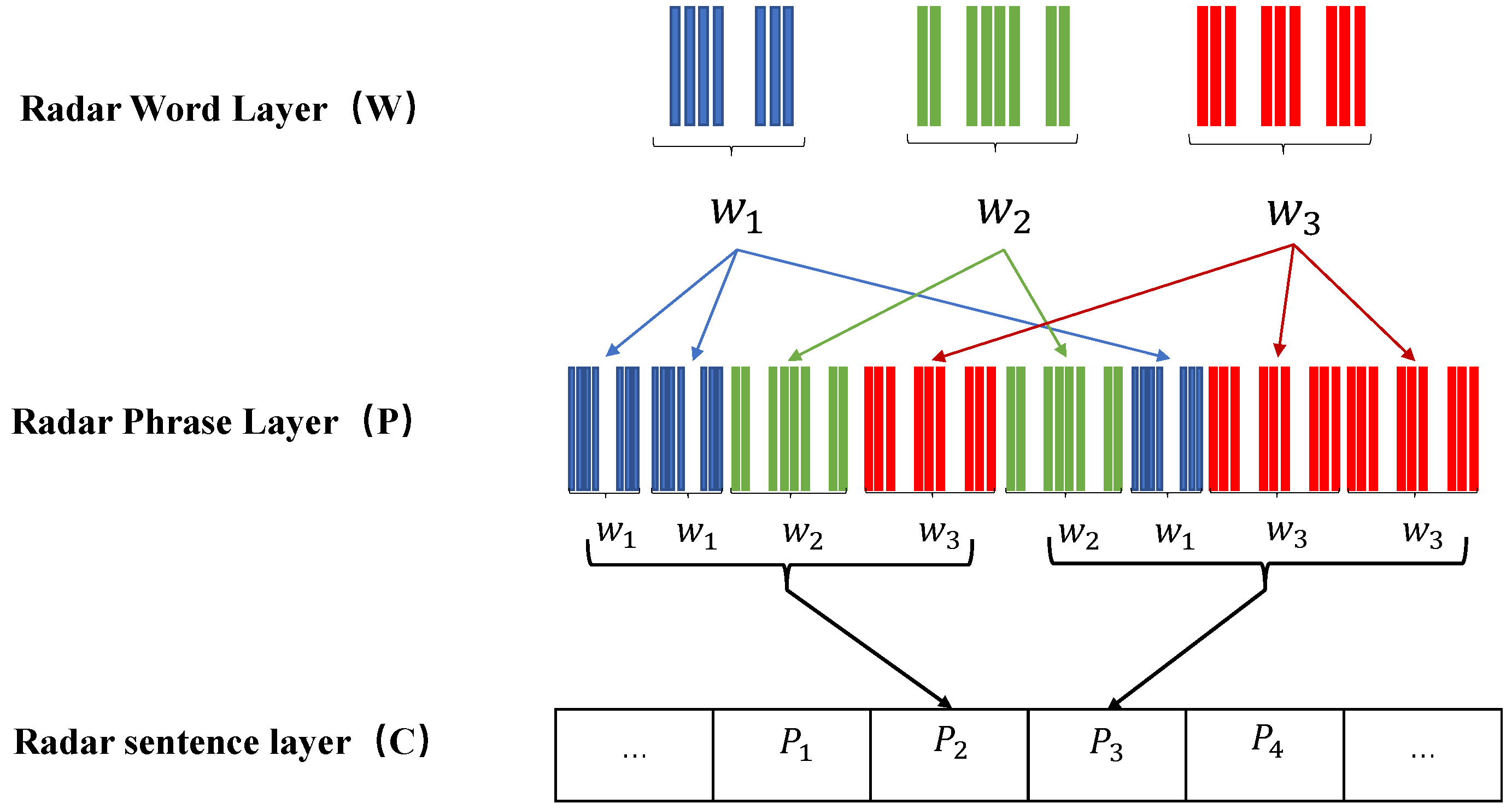
MFR Multi-Level Signal Model

In 2005, Haykin, Visnevski, and colleagues utilized Discrete Event System (DES) theory to analyze MFR signals at multiple levels and introduced a multi-level MFR signal structure model. This model provides a streamlined and effective approach for representing MFR signals. It enables hierarchical representation of MFR signals and formal depiction of signal generation and change rules [37].
In the MFR multi-level signal structure model, the fundamental unit is termed a radar word, which consists of a fixed sequence of radar pulses. A finite number of radar words are linked together to create a radar phrase, and several radar phrases are further connected to form a radar clause. This hierarchical structure facilitates the division of MFR signals into a symbolic system. For instance, as illustrated in Figure 1, the radar phrase ω 1 ω 1 ω 2 ω 3 is composed of a sequence of ω 1 , ω 2 , and ω 3 , and this phrase is subsequently connected with other radar phrases to form a radar sentence.
In Figure 2, the process of MFR generating signals according to the current task and grammar rules is shown. In this hierarchical MFR signal structure, the radar word layer is the most fundamental and basic unit for MFR signal analysis. Each radar phrase represents a specific function or task that the MFR can perform, such as search or tracking. The number of radar phrases within a radar sentence is closely linked to the scheduling cycle of the MFR, and the radar sentence reflects the current working mode of the radar. This hierarchical representation model of the MFR signal has the following characteristics:
(1) Each MFR working mode corresponds to multiple radar phrases, each performing different tasks. Additionally, some specific radar phrases may correspond to multiple working modes for various functions. Consequently, establishing a one-to-one correspondence between radar phrases and working modes is typically not feasible. Therefore, relying solely on radar phrases to identify radar working modes is inaccurate.
(2) The MFR working mode and radar phrases are usually multiplexed, and some errors may occur when extracting radar words from pulse sequences affected by noise factors. The above two aspects are the main sources of the final estimation error.
The advantage of using this MFR signal model for working mode recognition is that it decomposes the MFR signal into three hierarchical levels: radar words, radar phrases, and radar sentences. This decomposition limits the influence of different system-level laws to a single level, which simplifies the overall complexity of the system. Additionally, by employing formal grammar to describe the generation and change rules of MFR signals, the model ensures accuracy and consistency in representing MFR behavior. This rigorous mathematical framework provides a solid foundation for effective working mode recognition.

4. Model Architecture

4.1. CNN Modules

The modern architecture of CNN was developed by Yann LeCun and his colleagues for handwritten digit recognition. CNN models are more efficient and accurate than traditional machine learning algorithms, as they utilize local receptive fields and weight sharing mechanisms. CNN has the following advantages in radar signal processing:
(1) Local feature extraction and spatial information mining:
  • In radar signal processing, many key characters (such as frequency, pulse width, bandwidth, etc.) are manifested as local patterns of the signal. Through convolution operations, CNN can adaptively extract these local characters from radar signals, especially the frequency domain characters of the signal, which is crucial for the recognition of radar working modes. For example, for broadband radar signals, CNN can effectively identify the local high-frequency components in the signal to help distinguish different working modes.
(2) Adaptive filtering capability:
  • CNN has a natural filtering capability and can learn appropriate filters based on the characteristics of the input signal. It is highly robust to noise and interference. This is particularly important for the common noise problem in radar signal processing. CNN can automatically learn and remove irrelevant signal interference, extract cleaner and more useful pattern characters, and thus improve recognition accuracy.
The CNN structure is mainly composed of the following parts: input layer, convolution layer, ReLu layer, pooling layer and fully connected layer. By stacking these layers, a complete CNN can be constructed. The convolution layer is the core layer of CNN, which generates most of the calculations in the network and extracts and calculates local characters through its receptive field, and because convolution has the characteristic of weight sharing, it can reduce the number of parameters, reduce computing overhead, and prevent overfitting problems caused by too many parameters.

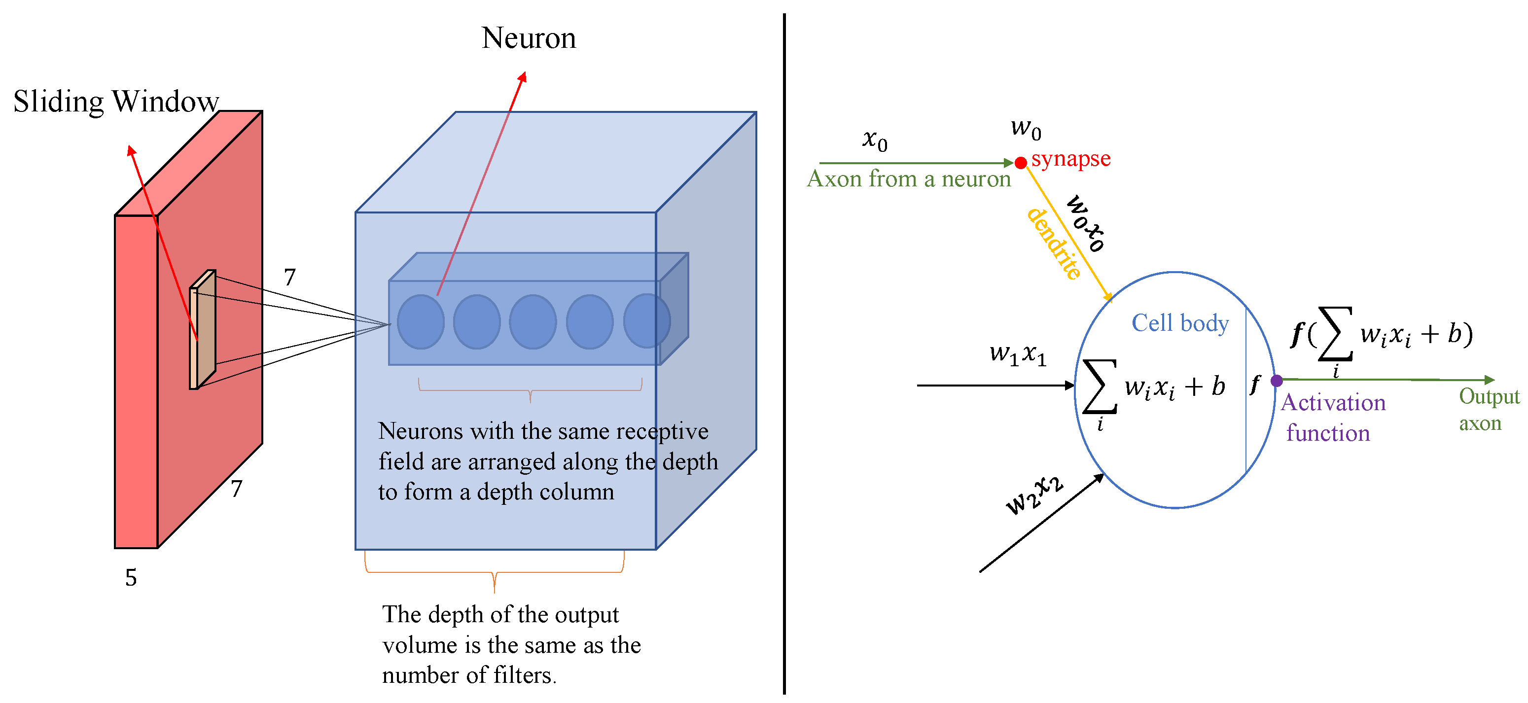
4.1.1. Receptive Field

When processing high-dimensional input data, it is not practical to use a fully connected neural network. On the contrary, if each neuron is connected to only a local area of the input data and different parts of the data are processed in parallel, calculations and feature extraction can be performed more efficiently. The spatial size of this connection is called the receptive field of the neuron. It should be noted that in the depth direction, the size of this connection is always equal to the depth of the input; that is, the connection is local in space (width and height), but in depth, it is always consistent with the depth of the input data.
The left side of Figure 3 shows a part of the CNN network, where the red is the input data, and the size of the input data in the figure is 7 × 7 × 5 . It should be noted that the size of the neuron in the depth dimension must also be 5, which is consistent with the depth of the input data body. The calculation form of each neuron in the CNN model is shown on the right side of Figure 3. It should be noted that no matter how many layers of input data there are, one convolution kernel only corresponds to one bias.

4.1.2. Spatial Arrangement of Neurons

The receptive field explains how each neuron in the convolutional layer is connected to the input data volume, but the number of neurons in the output data volume and how they are arranged have not yet been discussed. The size of the output data is mainly controlled by three hyperparameters: depth, stride, and zero-padding.
(1) The depth of the output volume is a hyperparameter that corresponds to the number of filters used, each of which looks for certain characters in the input data. As shown in the left part of Figure 3, a set of neurons arranged along the depth direction with the same receptive field is called a depth column.
(2) The stride controls how the filter performs convolution calculations around the input. The filter convolves the input by moving one unit at a time. The distance the filter moves is the stride. Figure 4 shows the output of a 7 × 7 input image passing through a 3 × 3 filter with strides of 1 and 3.
(3) Zero padding can control the spatial size of the output data volume. Since using filters for convolution will quickly reduce the spatial dimension, using zero padding can retain the information of the original input content as much as possible, thereby extracting the underlying characters and obtaining the size of the output data we need.
Therefore, the spatial size of the output data W 2 H 2 D 2 can be determined by the input data size and the spatial arrangement of neurons in the convolutional layer. The calculation formula is as follows:
W 2 = W 1 F + 2 P S + 1 H 2 = H 1 F + 2 P S + 1 D 2 = K
where F is the receptive field size, S is the stride, K is the number of filters, and P is the number of zero padding. Generally speaking, when the stride S = 1 , the zero padding value P = ( F 1 ) / 2 can ensure that the input and output data have the same spatial size.

4.2. Transformer Modules

The Transformer model is a deep learning framework proposed by Google in mid-2017. Compared with traditional sequence models (such as recurrent neural networks (RNNs)), it performs better in capturing long-distance dependencies and implementing parallel computing. The model introduces a self-attention mechanism to better handle long-distance dependencies and improve the training and reasoning efficiency of the model. Transformer has the following advantages in radar signal processing:
(1) Capturing long-term dependencies:
  • The working mode of radar signals is usually manifested as time-series data with long-term dependencies. These dependencies may span a long time window and have complex interactions with other parts of the signal. Transformer can effectively capture these global dependencies through the self-attention mechanism, which is particularly suitable for processing long time series data.
(2) Flexibility and scalability:
  • Unlike CNN, Transformer can directly perform weighted calculations on the input signal and adaptively adjust the weights of different signal parts, especially when the importance of information in different time periods in the signal is different. This makes Transformer highly adaptable and able to flexibly respond to dynamic changes in radar signals.
(3) Solving complex relationships between sequences:
  • The temporal changes in radar working modes usually have complex dependencies, and the various modes in the signal may have nonlinear interactions. Traditional neural networks may find it difficult to effectively model these complex relationships, while Transformer can comprehensively examine the relationship of the entire input sequence through the self-attention mechanism, not only focusing on local spatial information, but also understanding global temporal changes, providing richer contextual information for radar signal processing.
The model structure of Transformer is shown in Figure 5. Its overall architecture can be divided into three modules: input block, encoding-decoding block, and output block.

4.2.1. Input Block

The input block mainly consists of two parts, namely. the embedding layer and the positional encoding layer.
(1) Embedding Layer
The main function of the embedding layer is to map each word in the input text into a vector representation of a fixed size. Through embedding, high-dimensional data (such as text, categories, etc.) can be mapped to a low-dimensional continuous vector space. Such a representation is easier to be understood and processed by models such as neural networks, and can also capture the semantic relationships between data.
(2) Position Encoding Layer
Since each element in the input sequence is embedded into a word vector space after embedding, these embedding vectors themselves have no order information, so positional encoding is added to the model to provide position information to help the model capture the order information of the sequence. The encoding formula is as follows:
P E ( p o s , 2 i ) = sin p o s 10000 2 i / d m o d e l
P E ( p o s , 2 i + 1 ) = cos p o s 10000 2 i / d m o d e l
where p o s represents the position of the text in the text sequence, d model is the dimension of the embedding vector, i represents the position of the word embedding, the position encoding of the elements with odd position sequence numbers is represented by the cos function, and the even position sequence numbers are represented by the sin function. The encoding of each position obtained using the above encoding formula is unique, and the encodings of different dimensions have different frequencies, making it easier for the model to learn relative position information.

4.2.2. Encode Decode Block

The module mainly consists of two parts: the encoding module and the decoding module, and both are composed of N stacked encoders and decoders with the same structure.
(1) Multi-head attention mechanism
The multi-head attention mechanism consists of a self-attention layer, a connection layer, and a linear transformation layer. In the multi-head attention mechanism, the position-encoded input vector X is input into multiple self-attention networks, and the attention matrix of each network is calculated. First, three different linear projection matrices are initialized for the i-th self-attention network. After these three matrices are mapped into query W i Q , key W i K , and value W i V matrices, the results of each layer are calculated. The calculation process is as follows:
Q i = X W i Q K i = X W i K V i = X W i V H i = softmax ( Q i K i T d ) V i
In the formula, H i is the output result of the i-th self-attention network, d is the dimension of the three linear projection matrices, and the softmax function is used to limit the numerical range of the matrix. Then, the calculation results of multiple self-attention networks are spliced, the spliced results are processed through linear changes, and finally, the attention value matrix H is output as follows:
H = Concat ( H 1 , H 2 , , H i ) W
(2) Encoders and Decoders
Each encoder has two sublayers: the first layer is a multi-head attention mechanism, and the second layer is a fully connected feedforward neural network. Residual connections are used around each sublayer, followed by layer normalization. Each decoder has three sublayers. In addition to the two sublayers in the encoder, the decoder inserts a new sublayer that can perform a masked multi-head attention mechanism on the output embedding to prevent information leakage, and bias the output embedding to ensure that the current position can only depend on known outputs that are smaller than the current position.

4.2.3. Output Block

The output block is the key part of the entire model, responsible for converting the information processed by multiple layers of encoding and decoding into the final prediction results. For sequence classification tasks, the output layer includes pooling operations, linear transformations, Softmax layers, and cross entropy losses. Through these steps, the Transformer model is able to convert the processed information into the final prediction results.

4.3. Hybrid Model Architecture

Based on the analysis of the advantages of the above two models in radar signal processing, this paper considers a hybrid model of CNN and Transformer for radar working mode recognition.The hybrid model of MFR working mode recognition based on the CNN and Transformer model is shown in Figure 6. The overall framework of the model consists of two parts: a CNN local feature extraction block, and a simple Transformer global feature extraction block.
First, the data processed by the model is a radar PDW sequence after sorting. The shape of the model input data is (seq_length, num_words, num_features), where seq_length represents the sample length, that is, the number of radar phrases contained in each data, num_words represents the number of radar words contained in each radar phrase, and num_ characters indicates that each time step contains five characters. These data need to be dimensionally adjusted before being input into the CNN block. The data size is adjusted to (seq_length, num_features, num_words) to meet the input requirements of the convolution layer.
Then, the data are processed by the CNN Block, where the 1D convolutional layer extracts local characters from the signal, such as pulse width and frequency variation. The output of the convolutional layer is normalized by batch normalization, and then nonlinearity is added by the ReLU activation function. The computational complexity of CNN is low, which can effectively reduce the amount of input data for subsequent Transformer block, thereby improving overall computational efficiency.
The feature matrix output by the convolutional layer is then input to the Transformer block. In traditional Transformers, data are directly passed to the self-attention layer, which has a computational complexity of O ( n 2 ) , and has a high computational overhead when the sequence is long. The hybrid model extracts local characters through CNN, reducing the dimension of the Transformer input and reducing computational costs. The self-attention mechanism in the Transformer can capture global dependencies in the sequence and learn long-range relationships in the signal. In the Transformer Block, the data are first processed by a multi-head self-attention layer to capture the dependencies between time steps, and then the feature transformation is performed through a feedforward neural network. The model stability is improved and the training process is accelerated through skip connections and layer normalization techniques. Unlike traditional Transformers, the hybrid model reduces redundant information through CNN, thereby further reducing the computational burden of Transformers.
The output processed by the Transformer is reduced in dimension through pooling, and the time step characters are averaged and pooled using mean (dim = 0) to obtain a fixed-size feature vector. Pooling not only reduces the amount of calculation, but also avoids the problem of over-reliance on a single time step that may occur in traditional Transformers. Finally, the pooled characters are classified through a fully connected layer to output the prediction results of the radar working mode. The entire model combines local feature extraction and global dependency modeling to provide efficient and accurate pattern recognition capabilities.

5. Creation of Radar Dataset

Due to the sensitivity and confidentiality of radar technology, there is currently no available public data set for use and reference. The only available data mostly lists the range and rules of radar parameters, which are not closely aligned with the actual data. Based on the existing literature, this paper establishes a data set based on the Mercury radar. The data set mainly simulates the signal characteristics under different MFR working modes and adds the semantic information of the MFR signal scheduling logic to the data, and uses it to train and evaluate the performance of different models in radar signal processing and timing analysis.

5.1. Mercury MFR

The Mercury MFR is a real air defense radar. Its parameters and working mode information were made public in the literature by Dr. Fred A. Dilkes and others from Defence Research & Development Canada (DRDC) and used for algorithm verification. Although the public parameters have been declassified, they are still detailed and fully retain the characteristics of the radar’s behavior.
The Mercury MFR has nine radar words ( ω 1 ω 2 ω 9 ) , and the templates of each radar word are shown in Figure 7. Each radar word has a duration of 7.14 ms and consists of five parts A ~ E , where A, C, and E are silent times, B is a Doppler pulse sequence, and different radar words are distinguished by the PRI and pulse width of this part of the pulse. D is a synchronous pulse sequence with 12 pulses with a fixed PRI.
The Mercury radar has a total of five working modes:
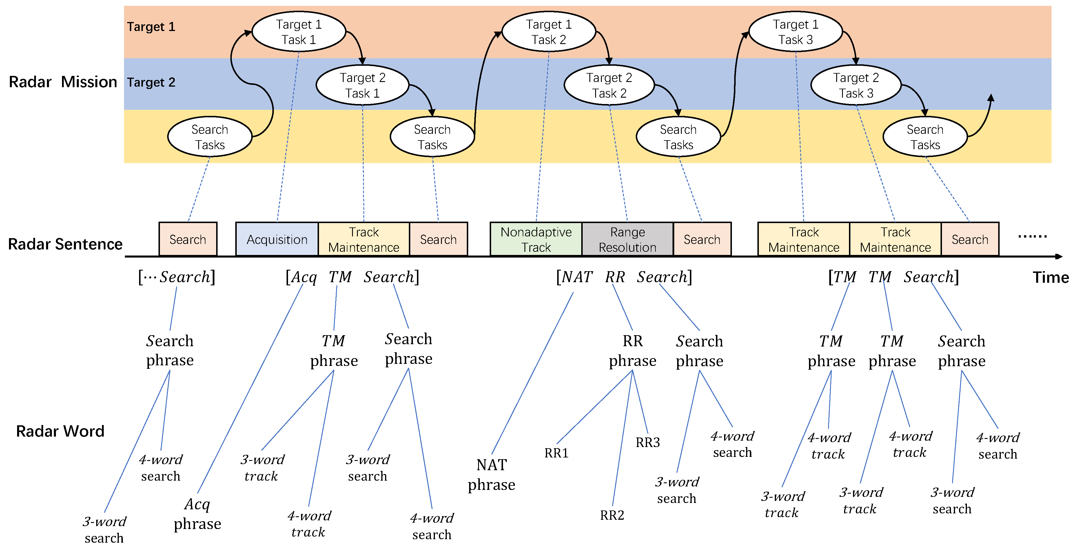
  • Search: This is one of the most basic working modes of MFR. The beam scans in a certain order in a specific airspace to detect unknown targets in a timely manner.
  • Acquisition (Acq): When a target is detected in search mode, the same radar word as the search signal is used to continuously illuminate the same direction at a higher data rate to confirm the detection result and complete the acquisition of the target.
  • Non-Adaptive Track (NAT): NAT is used for targets with a lower threat level. Search is dominant, and tracking does not occupy additional radar resources, that is, no special tracking beam is arranged. Instead, the search beam and data rate are used to detect the target to achieve a monitoring effect.
  • Range Resolution (RR): Alternately transmits multiple different PRF signals (radar words) to resolve range ambiguity and determine target location.
  • Track Maintenance (TM): When a target poses a high threat level, a dedicated beam is used to illuminate the target and keep tracking the target at a higher data rate.
Each working mode has several radar phrases to achieve its function. According to the literature [38], Table 1 is an important basis for generating the Mercury radar signal sequence based on syntax induction. The table comes from a simplified version of the intelligence analysis report.
From the table above, it can be seen that the radar phrases of the Mercury MFR are all composed of four radar words. The same radar phrase may be reused by different working modes, such as ( ω 1 ω 6 ω 6 ω 6 ) , ( ω 6 ω 6 ω 6 ω 6 ) , etc. A working mode may also use multiple different radar phrases according to the application scenario, such as the track-and-hold mode. MFR radar phrases are not randomly selected for use, but have their own rules. For example, in the search mode, during the dwell time of each wave position, the radar transmits a group of three or four radar words in a fixed order in a cycle; in the acquisition mode, the choice of radar phrase depends on the radar word used when searching for the target; and the non-adaptive tracking, range resolution and track-and-hold modes all have multiple radar phrases, representing signals of different PRFs. Selecting them in the optimized order can minimize the impact of range ambiguity and velocity ambiguity.

5.2. Radar Word Settings

Combined with the analysis of RWMR characteristic parameters in Section 3.1, we first select RF, PW, BW, PRI, and PA as characteristic parameters for radar working mode recognition, denoted as ω i = [ R F i , P W i , B W i , P R I i , P A i ] , where the subscript i represents the number of the i-th group of radar pulses detected in the pulse sequence in chronological order. Nine radar words are defined, and the range of the five characteristic parameters in each radar word is different. Each radar word sample is randomly generated within the given range. The parameter range is shown in Table 2:
It can be seen from the parameter range settings in the above table that there is a serious overlap in the variation ranges of the five characteristic parameters. In order to more intuitively display the overlap of the five characteristic parameters in the nine radar characters, the kernel density estimation (KDE) [39] method in statistics is used to estimate the probability density functions of several random variables to help understand the overlap and distribution characteristics between different data groups, and to more intuitively display the distribution of the data through a smooth curve.
Observing the KDE curves of the five characters in Figure 8, it can be seen that there is a clear separation in the frequency distribution of RF between different categories, especially in the higher and lower frequency bands. This shows that different categories can be distinguished by RF parameters. There is a large overlap in the distribution of PW, especially in the low pulse width region, indicating that it may be difficult to distinguish different categories on this parameter, but that some characters in the high pulse width region can help distinguish certain categories. The degree of overlap in the BW distribution is high, and this parameter has limited ability to distinguish certain categories. However, categories with specific BW (such as below 10 and above 20) may be relatively easy to distinguish. The KDE diagram of the PRI parameter shows the distribution of the pulse repetition interval. The distribution of most categories is concentrated in the lower PRI value range, and the overlap is serious. The distribution of the PA parameter shows a large overlap between different categories.
According to the literature [40], unsupervised learning in traditional machine learning is used to perform RWMR. The nine radar words established are classified using the clustering method. The two indicators of Adjusted Rand Index (ARI) and silhouette coefficient (SS) [41] are used to measure the quality of clustering results from different perspectives. The experimental results are as follows:
Three typical clustering algorithms are mainly used, namely, K-Means clustering, hierarchical clustering, and the DBSCAN clustering algorithm. From Figure 9, it can be seen intuitively that K-Means and hierarchical clustering both classify nine different clusters. The cluster boundaries of K-Means classification are clearer, and hierarchical clustering tends to cluster some dense data points together, but there is a certain ambiguity in the segmentation of clusters. The DBSCAN algorithm only classifies two clusters, indicating that the algorithm may not be able to effectively process the data set. ARI is an adjusted Rand index, which is mainly used to evaluate the similarity between two data partitions. It takes into account the influence of random partitioning, so the result range is [−1, 1]. The closer the ARI value is to 1, the higher the consistency between the clustering result and the true label. SS is used to evaluate the closeness of a single point to its cluster and the separation from other clusters. Its range is also [−1, 1]. The higher the SS value, the closer the points in the cluster are to each other and the clearer the separation from other clusters. Further combined with the indicator values in Table 3, it can be seen that the K-Means algorithm has the best classification performance among the three clustering algorithms, and DBSCAN has the worst performance and has no calculated value in the SS indicator. However, overall, the clusters classified by the clustering algorithm still have unclear boundaries and overlaps between different categories, and cannot effectively distinguish the nine radar words established.
From the above experimental results and analysis, it can be seen that since the nine radar characters have serious distribution overlap in different categories, it is difficult to effectively distinguish them through traditional clustering algorithms. This is closely aligned with the background that with the rapid development of phased array and cognitive technology, MFR has high flexibility in beam scheduling, resulting in a large number of overlaps in MFR waveform parameters. The parameter range setting of radar characters simulates the real confrontation situation well.

Creation of MFR-PDWS

According to the parameter range settings of the nine radar words established in Section 5.1 and the correspondence between the “Mercury” MFR radar phrases and their working modes in Table 1, the dataset MFR-PDWS is generated. Each piece of data in the data set is generated according to the flowchart logic of Figure 10. Each piece of data initially generated is 160 radar phrases, and then the sequence is randomly cut into a sequence of length 20 to simulate the randomness of the real battlefield reconnaissance process.
Considering that in the actual battlefield, real data often has complex time dependence, in order to simulate a real battlefield environment, the above generated data are subjected to time dependency calculation. Time dependency means that the data at a certain time point have a certain correlation with the data at the two previous and next time points. Time dependency is mainly introduced in two ways: short-term dependency and long-term dependency. The calculation formula is as follows:
P D W i = ( 1 α s h o r t ) P D W i + α s h o r t P D W i 1 i 1
P D W j = 1 k = 1 N α l o n g k P D W j + k = 1 N α l o n g k P D W j k j 4
In Formula (8), α _ s h o r t represents the short-term dependency ratio between the current PDW and the previous PDW. In Formula (9), N represents that the current PDW has a long-term dependency with the previous N PDWs, and the long-term dependency ratio is α _ l o n g . In this dataset, α _ s h o r t = 0.3 ,   k = 3 ,   α _ l o n g = 0.2 are taken. Only 100 samples are randomly generated for each working mode, totaling 700 samples.

6. Experiment and Result Analysis

This section mainly trains and verifies the performance of the established hybrid model in the radar working mode recognition task through experiments, and compares it with other models. The implementation of the algorithm and the construction of the neural network are written based on Python language and the Pytorch deep learning framework. The experimental simulation environment is built on Vscode 2024. The model parameters and specific experimental conditions in subsequent experiments are shown in Table 4.

6.1. Model Training Process

In the training phase, the cross entropy loss function is calculated by back propagation to optimize the model network parameters. The model optimizer selects the Adam optimizer. The data set contains 700 samples, each sample contains 20 × 4 time steps of PDW, and the sample dimension is 20 × 4 × 5. The training set and the test set are established in a ratio of 4:1, with a total of 560 training samples and 140 test samples.
The radar working mode recognition accuracy and loss curve during the model training process are shown in Figure 11. It can be seen from the figure that the model loss drops rapidly in the early stage of training (about 40 iterations), while the accuracy also rises rapidly, indicating that the model is learning quickly and effectively; after 70 cycles, the loss begins to stabilize and maintains at a low level, and the model accuracy approaches 100%, which means that the model has almost completely correctly classified the data on the training set. In the later stages of training, it can be noticed that there are some obvious spikes in the loss curve. The reason for this may be that due to the addition of certain mutations and outliers in the training data, the model will suddenly increase the loss when fitting these outliers. Although the loss fluctuates slightly in the later stages, it does not affect the excellent performance of the model on the training set.

6.2. Model Testing Results

After saving the model parameters trained in Section 6.1, we fixed the network parameters, and then loaded the saved parameters into the newly established hybrid model. We input the test data into the model and used the t-SNE technology to map the high-dimensional characters to the two-dimensional space, so that the classification of the model for different categories could be more intuitively seen in the two-dimensional space [42]. The following experimental results were obtained:
From the t-SNE dimension reduction visualization feature map in Figure 12, it can be seen that the model has extracted seven different characters, which is the same as the number of MFR working mode categories. The point clouds of different categories shown in the figure are separated from each other, forming obvious clusters, indicating that the model effectively extracts the characters of each category, so that different categories have good discrimination in high-dimensional space, and each category point data forms a relatively tight cluster in two-dimensional space. The higher the intra-class tightness, the stronger the model’s ability to represent the internal characters of the category. The model has consistency in feature extraction of the same category, which is beneficial to improving the robustness of the model; there are no obvious outliers in the figure, which indicates that the model has no obvious abnormal or misclassified data samples when extracting characters, indicating that the model has good stability and reliability. Further combined with the confusion matrix of the model in the test set, it can be seen that the model has achieved completely correct classification of the test set data, further verifying the excellent performance of the model in the radar working mode recognition task.

6.3. Comparison of the Model with Other Models

In this section, five models, namely, RNN, LSTM [26], GRUED [23], VGGnet, and ResNet, are selected for comparative experiments with the hybrid model proposed in this paper to verify the performance of different models in the radar working mode recognition task. The experiment records the change curves of the prediction accuracy of the six models during training as the training rounds and the classification accuracy in the test set, and generates statistics on the total time required for each model to complete all training rounds. The following experimental results are obtained:
First, from the accuracy comparison curves of each model training stage in Figure 13, we can intuitively see that ResNet and the hybrid model proposed in this article have an accuracy of nearly 100 % on the training set, VGGnet has an accuracy of 85.71 % , and the other three models perform poorly on the training set. Further combined with the accuracy comparison of each model in the training set and the test set in Table 5, it can be obtained that although ResNet can complete the classification of the data set well in the training phase, its prediction accuracy in the test set drops by 20 % , indicating that the model exhibits overfitting in the test set and the generalization performance of the model is not ideal. For VGGnet, which also has a high accuracy, combined with the training time statistics in Figure 14, it can be seen that due to the introduction of very deep convolutional layers in VGGnet, the training of the model requires a lot of time and computing resources, which is extremely disadvantageous in today’s rapidly changing electronic warfare battlefield. The three models of RNN, LSTM, and GRUED all perform poorly in classification accuracy and model training time. On the contrary, the hybrid model proposed in this paper achieves extremely high accuracy in both the training set and the test set, and also performs outstandingly in model training time. The comprehensive performance of the hybrid model is the best.
In order to conduct a more fine-grained analysis of the generalization performance of the model, evaluation indicators such as accuracy, recall, and F1 score were introduced, and the experimental results were obtained as shown in Figure 15. It can be clearly seen from the figure that the hybrid model has achieved significantly leading results in all three indicators, especially achieving the best balance between accuracy and recall. This balance is crucial for radar signal processing tasks in actual dynamic battlefield environments, because the model needs to ensure accuracy while not missing key signals in the face of noise, interference, and signal complexity.
The experimental results further verify the effectiveness of the hybrid model, especially in the analysis of high-dimensional complex signal data. The results show that it is superior to single models (such as RNN, LSTM, and GRU) and traditional convolutional models (VGGNet and ResNet), providing strong technical support for radar signal pattern recognition.

6.4. Ablation Experiment

In order to further verify the effectiveness of the model, understand the role of each module within the model, and improve the interpretability of the model, this section covers the performance of an ablation comparison experiment. According to Section 4 of this article, the model mainly consists of two modules: CNN and Transformer. First, the hybrid model is split. The structure of the model does not change. Only the output of the CNN module and the output of the Transformer module are adapted. The parameter settings of each model are still set according to Table 4. The three models are trained 300 times respectively, and the following experimental results are obtained:
From Table 6, we can see that among the three models, the hybrid model mentioned in the article has the best classification effect, with an accuracy of 97.14 % , followed by the Transformer model, and the CNN model has the worst performance, with an accuracy of only 58.57 % . Combining the confusion matrices of the three models in Figure 16, both the CNN and Transformer models have a certain degree of classification confusion for the TS and FS modes. This is because the types of radar words contained in the TS and FS modes are the richest. From Section 5.2, we can know that the parameter ranges of radar words in the dataset are highly overlapped, and a certain proportion of mutations and outliers are introduced into the dataset, which leads to a certain degree of misjudgment of the model’s recognition of radar words, which in turn makes the model’s classification performance for the TS and FS modes poor. For the classification of other modes, the performance of the Transformer model is better than that of the CNN model. This is because the Transformer can capture long-range dependencies, that is, the semantic information contained in the radar phrase scheduling logic. Therefore, compared with the CNN model that can only extract local temporal characters, it has a higher recognition accuracy in other radar working modes. The hybrid model fully combines the advantages of the two models in local and long-range feature extraction to achieve accurate classification of each mode.

6.5. Model Robustness Testing

In order to further explore the robustness of the model, missing PDW and spurious PDW are introduced to perform data augmentation operations on the test data set. Missing PDW means randomly setting the data in the data to zero; spurious PDW randomly generates the five feature parameters contained in the radar word, and the generation interval is the maximum variation range corresponding to the feature. For example, according to Table 2, the variation range of RF in the generated spurious PDW is [3000–11,000]. Then, the generated spurious PDW is randomly replaced with the PDW in the data according to a certain ratio. The variation range of the data ratio processed by the two data augmentations is 0–50%. The experiment is compared and tested on the basis of the model parameters trained and saved in Section 6.4, and the following experimental results are obtained:
According to Figure 17a, it can be seen that as the missing PDW ratio gradually increases, the accuracy of all models decreases. When the missing PDW ratio is 30 % , the hybrid model has a recognition accuracy of 90 % , and when the missing ratio is as high as 50 % , the hybrid model still has an accuracy of 70 % , while the recognition accuracy of other comparison models drops below 60 % ; Figure 17b shows the change curve of the accuracy of each model as the stray PDW ratio continues to increase. It can be seen intuitively from the figure that when the stray PDW ratio is higher than 5 % , the recognition accuracy of the five comparison models drops significantly, indicating that stray data has a serious impact on the recognition performance of the five comparison models. The hybrid model proposed in this paper begins to show a decline in recognition performance when the stray PDW ratio is higher than 20 % , and as the proportion of stray PDW continues to increase, the prediction accuracy gradually decreases, and finally the accuracy of the six models drops below 40 % . Through the above comparative experiments, it can be seen that the hybrid model proposed in this paper still has strong robustness compared with other models in harsh environments.

7. Conclusions

In view of the fact that the current MFR has high flexibility in waveform parameters and beam scheduling, making it increasingly difficult to establish a fixed relationship between MFR working modes, this paper proposes a RWMR method based on multi-feature joint learning. We combine the Transformer model, which has made great achievements in the field of natural language processing (NLP), with the CNN model that can perform efficient local feature extraction to form a lightweight hybrid model for RWMR. Additionally, based on the public literature and data, a dataset containing MFR scheduling grammar is established. The article first introduces several RWMR feature parameters and analyzes the change law of radar working mode feature parameters under different modes; secondly, the MFR multi-level signal model is introduced and the influence of each level on MFR behavior is analyzed. Then, the CNN module and Transformer module in the hybrid model are explained, and the overall model architecture is analyzed; finally, the model is built based on relevant data from the "Mercury" MFR, and five neural network models are selected for comparative experiments. The experiment proves the superiority of the hybrid model proposed in the article in the MFR working mode recognition task, and it is shown to still have good generalization performance and robustness when introducing a large number of missing PDWs and spurious PDWs.

Author Contributions

Conceptualization, L.L.; methodology, L.L.; software, L.L.; validation, L.L.; investigation, M.W.; writing—original draft preparation, L.L. and M.W.; writing—review and editing, L.L. and D.C.; funding acquisition, W.W. All authors have read and agreed to the published version of the manuscript.

Funding

This research was partially funded by the National Natural Science Foundation of China under Grants 61971429, 61871385, and 62471508, the Science and Technology Planning Project of the Guangdong Science and Technology Department under Grant Guangdong Key Laboratory of Advanced IntelliSense Technology (2019B121203006), and the Shenzhen Science and Technology Program under Grant KQTD20190929172704911.

Data Availability Statement

Data is contained within the article.

Conflicts of Interest

The authors declare no conflict of interest.

References

  1. Yuxin, F.; Jie, H.; Jiantao, W.; Tongxin, D.; Yiming, L.; Zhenyu, S. A review of multifunctional phased array radar behavior identification. Telecommun. Eng. 2024, 64, 643–654. [Google Scholar]
  2. Shafei, W.; Mengtao, Z.; Yunjie, L.; Jian, Y.; Yan, L. Identification, reasoning and prediction of advanced multifunctional radar system behavior: Review and prospect. Signal Process. 2024, 40, 17–55. [Google Scholar] [CrossRef]
  3. Yaoliu, Y.; Weigang, Z.; Shouye, L.; Hongyu, Z.; Yaoyan, H. A review of multifunctional radar working mode recognition methods. Telecommun. Eng. 2020, 60, 1384–1390. [Google Scholar]
  4. Shuaiying, Y.; Peng, P.; Yuan, R. Development Status and Trend of Shipborne Multifunctional Phased Array Radar. Ship Sci. Technol. 2023, 45, 141–147. [Google Scholar]
  5. Jian, O. Research on Multifunctional Radar Behavior Identification and Prediction Technology. Ph.D. Thesis, National University of Defense Technology, Changsha, China, 2017. [Google Scholar]
  6. Visnevski, N.; Dilkes, F.; Haykin, S.; Krishnamurthy, V. Non-self-embedding context-free grammars for multi-function radar modeling–electronic warfare application. In Proceedings of the IEEE International Radar Conference, Arlington, VA, USA, 9–12 May 2005; pp. 669–674. [Google Scholar] [CrossRef]
  7. Ya, S.; Wenbo, Z.; Mingzhe, Z.; Lei, W.; Shengjun, X. A review of radar emitter individual identification. J. Electron. Inf. Technol. 2022, 44, 2216–2229. [Google Scholar]
  8. Wang, J.; Zheng, T.; Lei, P.; Wei, S. A review of deep learning in radar. J. Radar 2018, 7, 395–411. [Google Scholar]
  9. Yu, K.; Qi, Y.; Shen, L.; Wang, X.; Quan, D.; Zhang, D. Radar Signal Recognition Based on Bagging SVM. Electronics 2023, 12, 4981. [Google Scholar] [CrossRef]
  10. Zhou, Z.; Fei, W.; Zheng, F.; Luo, J. A Radar Working Mode Recognition Algorithm with Approximate Coherent Metric and Multi-Agent PSR Model. In Proceedings of the 12th International Conference on Computer Engineering and Networks, Haikou, China, 4–7 November 2022; Liu, Q., Liu, X., Cheng, J., Shen, T., Tian, Y., Eds.; Springer: Singapore, 2022; pp. 456–465. [Google Scholar] [CrossRef]
  11. Lang, P.; Fu, X.; Martorella, M.; Dong, J.; Qin, R.; Meng, X.; Xie, M. A Comprehensive Survey of Machine Learning Applied to Radar Signal Processing. arXiv 2020, arXiv:2009.13702. [Google Scholar]
  12. Ou, J.; Chen, Y.; Zhao, F.; Liu, J.; Xiao, S. Novel Approach for the Recognition and Prediction of Multi-Function Radar Behaviours Based on Predictive State Representations. Sensors 2017, 17, 632. [Google Scholar] [CrossRef] [PubMed]
  13. Ou, J.; Chen, Y.; Zhao, F.; Liu, J.; Xiao, S. Method for operating mode identification of multi-function radars based on predictive state representations. IET Radar Sonar Navig. 2017, 11, 426–433. [Google Scholar] [CrossRef]
  14. Chi, K.; Shen, J.; Li, Y.; Wang, L.; Wang, S. A novel segmentation approach for work mode boundary detection in MFR pulse sequence. Digit. Signal Process. 2022, 126, 103462. [Google Scholar] [CrossRef]
  15. Geng, Z.; Yan, H.; Zhang, J.; Zhu, D. Deep-Learning for Radar: A Survey. IEEE Access 2021, 9, 141800–141818. [Google Scholar] [CrossRef]
  16. Liu, L.; Li, X. Radar signal recognition based on triplet convolutional neural network. EURASIP J. Adv. Signal Process. 2021, 2021, 112. [Google Scholar] [CrossRef]
  17. Shao, G.; Chen, Y.; Wei, Y. Convolutional neural network-based radar jamming signal classification with sufficient and limited samples. IEEE Access 2020, 8, 80588–80598. [Google Scholar] [CrossRef]
  18. Gao, J.; Shen, L.; Gao, L. Modulation recognition for radar emitter signals based on convolutional neural network and fusion features. Trans. Emerg. Telecommun. Technol. 2019, 30, e3612. [Google Scholar] [CrossRef]
  19. Wang, L.; Yang, X.; Tan, H.; Bai, X.; Zhou, F. Few-shot class-incremental SAR target recognition based on hierarchical embedding and incremental evolutionary network. IEEE Trans. Geosci. Remote Sens. 2023, 61, 1–11. [Google Scholar] [CrossRef]
  20. Geng, J.; Wang, H.; Fan, J.; Ma, X. SAR Image Classification via Deep Recurrent Encoding Neural Networks. IEEE Trans. Geosci. Remote Sens. 2018, 56, 2255–2269. [Google Scholar] [CrossRef]
  21. Li, X.; Liu, Z.; Huang, Z.; Liu, W. Radar Emitter Classification With Attention-Based Multi-RNNs. IEEE Commun. Lett. 2020, 24, 2000–2004. [Google Scholar] [CrossRef]
  22. Xu, X.; Bi, D.; Pan, J. Method for functional state recognition of multifunction radars based on recurrent neural networks. IET Radar Sonar Navig. 2021, 15, 724–732. [Google Scholar] [CrossRef]
  23. Chen, H.; Feng, K.; Kong, Y.; Zhang, L.; Yu, X.; Yi, W. Multi-Function Radar Work Mode Recognition Based on Encoder-Decoder Model. In Proceedings of the IGARSS 2022–2022 IEEE International Geoscience and Remote Sensing Symposium, Kuala Lumpur, Malaysia, 17–22 July 2022; pp. 1189–1192. [Google Scholar] [CrossRef]
  24. Chen, H.; Feng, K.; Kong, Y.; Zhang, L.; Yu, X.; Yi, W. Function Recognition Of Multi-function Radar Via CNN-GRU Neural Network. In Proceedings of the 2022 23rd International Radar Symposium (IRS), Gdansk, Poland, 12–14 September 2022; pp. 71–76. [Google Scholar] [CrossRef]
  25. Apfeld, S.; Charlish, A. Recognition of Unknown Radar Emitters With Machine Learning. IEEE Trans. Aerosp. Electron. Syst. 2021, 57, 4433–4447. [Google Scholar] [CrossRef]
  26. Li, Y.; Zhu, M.; Ma, Y.; Yang, J. Work modes recognition and boundary identification of MFR pulse sequences with a hierarchical seq2seq LSTM. IET Radar Sonar Navig. 2020, 14, 1343–1353. [Google Scholar] [CrossRef]
  27. Liu, Z.M. Recognition of Multifunction Radars Via Hierarchically Mining and Exploiting Pulse Group Patterns. IEEE Trans. Aerosp. Electron. Syst. 2020, 56, 4659–4672. [Google Scholar] [CrossRef]
  28. Li, X.; Liu, Z.; Huang, Z. Attention-Based Radar PRI Modulation Recognition With Recurrent Neural Networks. IEEE Access 2020, 8, 57426–57436. [Google Scholar] [CrossRef]
  29. Tian, T.; Zhang, Q.; Zhang, Z.; Niu, F.; Guo, X.; Zhou, F. Shipborne Multi-Function Radar Working Mode Recognition Based on DP-ATCN. Remote Sens. 2023, 15, 3415. [Google Scholar] [CrossRef]
  30. Li, X.; Cai, Z. Deep Learning and Time-Frequency Analysis Based Automatic Low Probability of Intercept Radar Waveform Recognition Method. In Proceedings of the 2023 IEEE 23rd International Conference on Communication Technology (ICCT), Wuxi, China, 20–22 October 2023; pp. 291–296. [Google Scholar] [CrossRef]
  31. Wang, C.; Wang, J.; Zhang, X. Automatic radar waveform recognition based on time-frequency analysis and convolutional neural network. In Proceedings of the 2017 IEEE International Conference on Acoustics, Speech and Signal Processing (ICASSP), New Orleans, LA, USA, 5–9 March 2017; pp. 2437–2441. [Google Scholar] [CrossRef]
  32. Wei, C.; Wang, Z.; Xiong, S.; Zhang, Y. ISAR Target Recognition Method Based on Time-Frequency Two-Dimensional Joint Domain Adversarial Learning Network. In Proceedings of the 2023 Cross Strait Radio Science and Wireless Technology Conference (CSRSWTC), Guilin, China, 10–13 November 2023; pp. 1–3. [Google Scholar] [CrossRef]
  33. Feng, K.; Chen, H.; Kong, Y.; Zhang, L.; Yu, X.; Yi, W. Prediction of Multi-Function Radar Signal Sequence Using Encoder-Decoder Structure. In Proceedings of the 2022 7th International Conference on Signal and Image Processing (ICSIP), Suzhou, China, 20–22 July 2022; pp. 152–156. [Google Scholar] [CrossRef]
  34. Zhai, Q.; Li, Y.; Zhang, Z.; Li, Y.; Wang, S. Few-Shot Recognition of Multifunction Radar Modes via Refined Prototypical Random Walk Network. IEEE Trans. Aerosp. Electron. Syst. 2023, 59, 2376–2387. [Google Scholar] [CrossRef]
  35. Zhang, Z.; Li, Y.; Zhai, Q.; Li, Y.; Gao, M. Few-Shot Learning for Fine-Grained Signal Modulation Recognition Based on Foreground Segmentation. IEEE Trans. Veh. Technol. 2022, 71, 2281–2292. [Google Scholar] [CrossRef]
  36. Juyuan, Z. Research and Application of Radar Working Mode Recognition Based on Machine Learning. Master’s Thesis, Beijing University of Posts and Telecommunications, Beijing, China, 2021. [Google Scholar]
  37. Shuang, Z. Research on key technologies of multi-function radar electronic intelligence signal processing. Electron. Qual. 2019, 1, 2–23. [Google Scholar]
  38. Visnevski, N.; Krishnamurthy, V.; Wang, A.; Haykin, S. Syntactic Modeling and Signal Processing of Multifunction Radars: A Stochastic Context-Free Grammar Approach. Proc. IEEE 2007, 95, 1000–1025. [Google Scholar] [CrossRef]
  39. Gallego, J.A.; Osorio, J.F.; Gonzalez, F.A. Fast kernel density estimation with density matrices and random fourier features. In Proceedings of the Ibero-American Conference on Artificial Intelligence; Springer: Cham, Switzerland, 2022; pp. 160–172. [Google Scholar] [CrossRef]
  40. Longjun, Z.; Bo, D.; Weijian, S.; Shan, G. Multi-function radar working mode recognition based on cluster analysis method. Ship Electron. Eng. 2022, 42, 86–88. [Google Scholar]
  41. Su, X.; Xue, S.; Liu, F.; Wu, J.; Yang, J.; Zhou, C.; Hu, W.; Paris, C.; Nepal, S.; Jin, D.; et al. A Comprehensive Survey on Community Detection With Deep Learning. IEEE Trans. Neural Netw. Learn. Syst. 2024, 35, 4682–4702. [Google Scholar] [CrossRef] [PubMed]
  42. Sun, Y.; Han, Y.; Fan, J. Laplacian-based Cluster-Contractive t-SNE for High-Dimensional Data Visualization. ACM Trans. Knowl. Discov. Data 2023, 18, 22. [Google Scholar] [CrossRef]
Figure 1. MFR multi-level signal structure model.
Remotesensing 17 00521 g001
Figure 2. MFR signal generation process.
Remotesensing 17 00521 g002
Figure 3. CNN receptive field connection and size description.
Remotesensing 17 00521 g003
Figure 4. Convolution stride.
Remotesensing 17 00521 g004
Figure 5. Transformer Model Architecture.
Remotesensing 17 00521 g005
Figure 6. Hybrid model framework diagram.
Remotesensing 17 00521 g006
Figure 7. Mercury MFR radar word template.
Remotesensing 17 00521 g007
Figure 8. Comparison of KDE plots for different characters.
Remotesensing 17 00521 g008
Figure 9. Clustering result diagram.
Remotesensing 17 00521 g009
Figure 10. Data generation logic.
Remotesensing 17 00521 g010
Figure 11. Comparison of model loss and accuracy during training.
Remotesensing 17 00521 g011
Figure 12. Test results.
Remotesensing 17 00521 g012
Figure 13. Model accuracy comparison curve.
Remotesensing 17 00521 g013
Figure 14. Model training time comparison bar chart.
Remotesensing 17 00521 g014
Figure 15. Comparison of accuracy, recall, and F1 scored.
Remotesensing 17 00521 g015
Figure 16. Confusion matrices. (a) CNN. (b) Transformer. (c) Hybrid.
Remotesensing 17 00521 g016
Figure 17. Data augmentation experimental results. (a) Missing pulse; (b) Spurious pulse.
Remotesensing 17 00521 g017
Table 1. Mercury MFR working modes and radar phrases [38].
Working ModePhaseWorking ModePhase
Search4-Word Serrch
(FS)
[ ω 1 ω 2 ω 4 ω 5 ] Track Maintenance
(TM)
4-Word Track
(FT)
[ ω 7 ω 7 ω 7 ω 7 ]
[ ω 2 ω 4 ω 5 ω 1 ] [ ω 8 ω 8 ω 8 ω 8 ]
[ ω 4 ω 5 ω 1 ω 2 ] [ ω 9 ω 9 ω 9 ω 9 ]
[ ω 5 ω 1 ω 2 ω 4 ] 3-Word Track
(ST)
[ ω 1 ω 7 ω 7 ω 7 ]
3-Word Serrch
(TS)
[ ω 1 ω 3 ω 5 ω 1 ] [ ω 2 ω 7 ω 7 ω 7 ]
[ ω 3 ω 5 ω 1 ω 3 ] [ ω 3 ω 7 ω 7 ω 7 ]
[ ω 5 ω 1 ω 3 ω 5 ] [ ω 4 ω 7 ω 7 ω 7 ]
Nonadaptive Track
(ANT)
[ ω 1 ω 6 ω 6 ω 6 ] [ ω 5 ω 7 ω 7 ω 7 ]
[ ω 2 ω 6 ω 6 ω 6 ] [ ω 6 ω 7 ω 7 ω 7 ]
[ ω 3 ω 6 ω 6 ω 6 ] [ ω 7 ω 7 ω 7 ω 7 ]
[ ω 4 ω 6 ω 6 ω 6 ] [ ω 1 ω 8 ω 8 ω 8 ]
[ ω 5 ω 6 ω 6 ω 6 ] [ ω 2 ω 8 ω 8 ω 8 ]
[ ω 6 ω 6 ω 6 ω 6 ] [ ω 3 ω 8 ω 8 ω 8 ]
Acquisition
(Acq)
[ ω 2 ω 2 ω 2 ω 2 ] [ ω 4 ω 8 ω 8 ω 8 ]
[ ω 3 ω 3 ω 3 ω 3 ] [ ω 5 ω 8 ω 8 ω 8 ]
[ ω 4 ω 4 ω 4 ω 4 ] [ ω 6 ω 8 ω 8 ω 8 ]
[ ω 5 ω 5 ω 5 ω 5 ] [ ω 8 ω 8 ω 8 ω 8 ]
[ ω 6 ω 6 ω 6 ω 6 ] [ ω 1 ω 9 ω 9 ω 9 ]
Range Resolution
(RR)
RR1 [ ω 1 ω 6 ω 6 ω 6 ] [ ω 2 ω 9 ω 9 ω 9 ]
[ ω 7 ω 6 ω 6 ω 6 ] [ ω 3 ω 9 ω 9 ω 9 ]
RR2 [ ω 3 ω 6 ω 6 ω 6 ] [ ω 4 ω 9 ω 9 ω 9 ]
[ ω 8 ω 6 ω 6 ω 6 ] [ ω 5 ω 9 ω 9 ω 9 ]
RR3 [ ω 5 ω 6 ω 6 ω 6 ] [ ω 6 ω 9 ω 9 ω 9 ]
[ ω 9 ω 6 ω 6 ω 6 ] [ ω 9 ω 9 ω 9 ω 9 ]
Table 2. RWMR characteristic parameter range.
RFPWBWPRIPA
ω 1 3000–360015–305–10300–500−10–7
ω 2 3400–40000.5–201–7100–400−5–0
ω 3 4000–46002–1012–1650–1500–3
ω 4 4400–50000.5–106–1550–250−3–0
ω 5 9900–11,00015–3010–184000–6000−5–5
ω 6 9200–960010–2215–27800–20000–3
ω 7 9600–99000.5–24–12400–1000−1–7
ω 8 9600–11,00012.5–202–2050–5002–10
ω 9 3000–450015–209–183000–4500−5–0
Table 3. Clustering effect comparison.
ARISS
K-means0.5803220.389653
Agglomerative0.4802690.38024
DBSCAN0.123411N/A
Table 4. Experimental conditions and model parameter settings table.
ModulesParameterValueModulesParameterValue
Hardware ResourcesProcessorInter CORE i7-12700F, 2 ~ .1GTramsformer d r o p _ o u t 0.1
Memory16384MB(RAM) h e a d _ n u m 4
GraphicsNVIDIA GeForce GT 730 f f n _ d i m 128
Hyperparameter n u m _ f e a t u r e s 5VGGnet z e r o _ p a d d i n g 1
s e q _ l e n g t h 80 k e r n e l _ s i z e 3
l e a r n i n g r a t e 0.001 s t r i d e 1
b a t c h _ s i z e 64 l a y e r _ n u m 15
n u m _ e p o c h 300Restnet d r o p _ o u t 0.1
c l a s s _ n u m 7 k e r n e l _ s i z e 3
CNN-Bclock k e r n e l _ s i z e 3 s t r i d e 1
s t r i d e 1 z e r o _ p a d d i n g 1
z e r o _ p a d d i n g 1GRUED D e c o d e _ l a y e r 3
LSTM h i d d e n _ s i z e 64 h i d d e n _ s i z e 64
RNN h i d d e n _ s i z e 64 E n c o d e _ l a y e r 3
Table 5. Comparison of model training and test experiment accuracy.
ModelRNNLSTMGRUEDHybridVGGnetResNet
Train-accuracy 34.55 % 43.37 % 78.59 % 98.13 % 85.71 % 99.2 %
Test-accuracy 37.41 % 47.86 % 39.29 % 99.28 % 84.28 % 81.0 %
Table 6. Ablation experiment results.
CNN-BlockTransformer-BlockAccuracy
CNN Model× 58.57 %
Transformer Model× 90.00 %
Hybri Model 97.14 %
Disclaimer/Publisher’s Note: The statements, opinions and data contained in all publications are solely those of the individual author(s) and contributor(s) and not of MDPI and/or the editor(s). MDPI and/or the editor(s) disclaim responsibility for any injury to people or property resulting from any ideas, methods, instructions or products referred to in the content.

