Abstract
The strong Antarctic vortex plays a crucial role in forming an expansive region with significant stratospheric ozone depletion during austral spring, commonly referred to as the Antarctic “ozone hole”. This study examines daily ozone column behavior during this phenomenon using ERA5 reanalysis data and ground-based observations from 10 Antarctic stations collected between September and December from 2008 to 2022. A preliminary analysis of these datasets revealed smoothly varying patterns with quasi-uniform gradients in the ozone distribution within the ozone hole. This observation led to the hypothesis that average ozone columns over zones, defined as concentric areas around the South Pole, can be estimated using mean values of the measurements derived from station observations. This study aims to evaluate the validity of this hypothesis. The results indicate that the mean ozone levels calculated from daily measurements at two stations—Belgrano and Dome Concordia, or Belgrano and Arrival Heights—provide a reliable approximation of the average ozone levels over the zone spanning 70°S to 90°S. Including additional stations extended the zone of reliable approximation northward to 58°S. The approximation error was estimated to range from 5% to 7% at 1σ and from 6% to 8% at the 10th–90th percentile levels. Furthermore, the geographical distribution of the stations enabled a schematic reconstruction of the ozone hole’s position and shape. On the other hand, the high frequency of ground-based measurements contributed to studying the ozone hole variability in both the inner area and edges on an hourly time scale. These findings have practical implications for the near-real-time monitoring of ozone hole development, along with satellite observations, considering ground-based measurements as a source of information about ozone layer in the South Pole region. The results also suggest the possible role of observations from the ground in the analyses of pre-satellite-era hole behavior. Additionally, this study found a high degree of consistency between ground-based measurements and corresponding ERA5 reanalysis data, further supporting the reliability of the observations.
1. Introduction
Following the discovery of ozone in the mid-19th century, understanding its role in atmospheric processes rapidly advanced over the subsequent years, alongside the development of instruments for measuring its atmospheric content [1,2,3,4,5,6,7,8,9,10,11]. In 1920, Fabry and Buisson [6] developed a spectrograph to measure solar ultraviolet (UV) irradiance at the Earth’s surface and conducted the first assessment of the ozone column consistent with modern estimates. Their method to extract the ozone amount, which involved comparing UV irradiances at two wavelengths—one strongly absorbed by the ozone and the other less affected—remains in use today. They estimated the ozone column at Paris to vary around 0.3 atm. cm in May and June 1920. Later, the Dobson Unit (1 DU = 10−3 atm. cm = 2.69 1016 molecules/cm2) was introduced to measure the ozone amount in an atmospheric column. In the first half of the 20th century, atmospheric ozone measurements intensified after the construction of the Dobson spectrophotometer [11]. The number of stations equipped with this instrument increased to 32 at the beginning of the International Geophysical Year 1957/58. A fully automated Brewer spectrophotometer was designed for measuring the ozone column in the 1970s, and it has been routinely used since the 1980s [12,13]. Dobson and Brewer instruments both derive the ozone column using the methods outlined in [6], with accuracy assessed to be approximately 1% under clear skies [13,14]. Differential Optical Absorption Spectroscopy (DOAS) enabled the development of an additional procedure for assessing the ozone column in the second half of the last century [15,16], which necessitated a modification of the corresponding spectrophotometers. This approach is applied in ground-based [17,18,19], balloon-born [20], aircraft [21,22], and satellite measurements [23,24]. In recent years, the assimilation of data provided by both satellite and ground-based devices has led to the assembling of large databases where the total ozone column distribution around the world can be found with high spatial resolution [25,26].
The first assessments of the ozone column in the polar regions [11] highlighted a substantial difference between the Northern and Southern hemispheres. It is interesting to observe that looking at the first results from Halley Bay (75°34’S 25°30’W) collected in the austral spring of 1956, Dobson and his collaborators [11] had doubts about the instrument’s correct operation since the ozone was lower compared to the amounts at Spitzbergen during the boreal spring period. After similar results obtained in successive years confirmed such behavior, Dobson rightly assumed that the stronger polar vortex in the Southern hemisphere could cause the observed difference. Initial measurements at Halley Bay between 1956 and 1958 revealed a minimum ozone column of 250–280 DU during the austral spring period, while corresponding values in the Arctic during the boreal spring period were estimated at nearly 450 DU [11]. A notable decline in ozone minima was observed in the 1980s [27,28], marking the Antarctic ozone as a critical focus in atmospheric research [29,30,31,32,33,34,35].
Advancements in space-borne instruments enhanced our understanding of the ozone depletion over Antarctica, a phenomenon now known as the “ozone hole”. (The term “ozone hole” adopted in both the popular and scientific literature will be used in this text to indicate the ozone-depleted area covering Antarctica in the austral spring period.) [36,37,38,39,40,41,42,43]. Ozone depletion usually starts in late winter following the development of the polar vortex that isolates a large area in the stratosphere over the Antarctic continent and creates conditions for strong stratospheric cooling. When the temperature drops below 195 K, polar stratospheric clouds begin to form, which are crucial for chemical ozone destruction [31,44,45,46]. The Antarctic ozone hole appears in September when returning sunlight leads to catalytic chemical ozone destruction and reaches its deepest state between late September and early October with ozone columns of 100–180 DU. The breakup of the hole typically starts in late October or early November, followed by the ozone column’s recovery to the normal level of more than 300 DU in November–December. It is generally agreed to define the Antarctic ozone hole as the area where the ozone column does not exceed 220 DU [31]. The hole is characterized by an oval shape covering an area of 20–25 million square kilometers [31,47], usually including the whole continent. Over the past few decades, an equatorward shift in the ozone hole in the Atlantic sector has been observed and has been accounted for by a change in planetary wave activity. This shift has created a certain asymmetry in the zonal ozone distribution in Antarctica [48,49,50,51,52], resulting in the cooling of the stratosphere and upper troposphere that has significantly affected the South Hemisphere’s climate [29].
Similar deep ozone depletions are not typically observed in the Arctic, where the ozone column usually reaches its maximum in the boreal spring. Areas with a reduced ozone content are limited and occur only sporadically, as the different atmospheric dynamics in relation to the Antarctic result in a smaller and less stable polar vortex. Nevertheless, several episodes of deeper ozone depletion have also taken place in the Arctic during the past two decades [53,54].
Modern satellite technologies and data processing methods enable the precise acquisition of high-resolution ozone column distributions over the polar regions. The construction of such distribution maps is a helpful activity for studying large-scale stratospheric dynamics, taking into account the polar regions’ role in global atmospheric processes. In this context, the present study aims to propose an alternative approach to achieve an entire approximate picture of the ozone column over Antarctica using ground-based measurements. An important advantage of these observations is their ability to provide information about very short-period variations in the ozone column within an hourly timescale. This allows the short-term variability in the stratosphere to be examined. Along with a discussion of this advantage, the assumption of approximately assessing the average ozone column over zones determined as concentric areas around the South Pole through ground-based observations is examined. Furthermore, the possibility of reconstructing a schematic ozone hole image is also discussed. These approximations are considered an addition to satellite techniques and provide an opportunity for a deeper study of the ozone hole, and they could also play a certain role in the analyses of pre-satellite-era data.
2. Data and Methods
Two datasets were used in the present study. The first set consisted of ground-based measurements taken at 10 Antarctic stations, where relatively continuous monitoring of the ozone column has been carried out within the past 15 years. Figure 1 shows the locations of the stations considered, and Table 1 summarizes their coordinates and the equipment used. Data for seven of the stations were taken from the World Ozone and Ultraviolet Radiation Data Centre (WOUDC) [55] database, while the measurements at the three other stations were provided by the respective teams overseeing the instrumentation. Nine stations were equipped with the widely used Dobson, Brewer, and SAOZ [17] photometers, while the data from the Dome Concordia station were collected by the narrow-band filter radiometer UV-RAD [56]. The period between 2008 and 2022, which covers available ground-based data, was chosen for analysis. Moreover, only the months from September to December, which span the development and dissipation of the ozone hole, were taken into account. Table 1 presents the most significant gaps in the ground-based dataset.
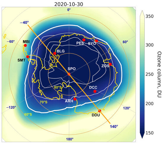
Figure 1.
The ground-based stations included in the present study are identified by their GAW ID (see Table 1). The background represents the ozone column distribution constructed from the ERA5 dataset for the day indicated on the map. The thick white curve outlines the ozone hole edges (the area with an ozone column lower than 220 DU), while the thin white curves present the areas with an ozone column less than 180, 150, and 140 DU from the edge to the inner regions, respectively. The orange line determined by −40° and 140° meridians approximately depicts the strip covered by most stations.

Table 1.
The ground-based stations providing data for this study. The corresponding Global Atmosphere Watch (GAW) identification (ID) code for each station is also given, together with the geographical coordinates and instruments. The last column exhibits the main gaps in the data within the adopted period (September–December 2008–2022).
The second dataset was extracted from the ERA5 reanalysis conducted by the European Center for Medium-Range Weather Forecasts (ECMWF), where the ozone column over the globe with spatial resolution in both latitude and longitude can be found with a 1-h temporal step [57]. Ozone amounts within the 40°S–90°S range were retrieved for the selected period over an expanded latitude–longitude grid of which enables faster computations, keeping an acceptable spatial resolution [57]. The daily mean values were calculated by averaging the ozone columns at 00:00, 04:00, 08:00, 12:00, 16:00, and 20:00 for each day, assuming this sampling can provide realistic estimates of the mean amount. The time series for each grid point contains 1830 values.
The aim of the study is to compare different parameters by calculating the ratios between them and examining the extent of the closeness of to 0 or 1 depending on the concrete definition. Standard statistics approaches [58], briefly listed below, were used in the analysis.
A histogram is a widely used tool for resolving various statistical problems. Let us assume that the studied ratio is determined as a sequence defined over an interval , where and are real numbers close to 1. If we cover by subintervals , named as bins, each with a width of , the histogram given the probability to be within can be defined as follows:
where the delta-function is determined as follows:
The histogram defined through Equations (1) and (2) gives the relative distribution of over . The cumulative distribution function (CDF) is defined as follows:
The function represents the probability of being inferior to the right bound of as a percentage. The fractiles , also known as percentiles, bind submanifolds of that can appear with probability , which can be calculated from the following equation [58]:
In practice, the median , which is equal to corresponding to half of CDF, is widely used in data analysis.
Figure 2 shows a histogram of a hypothetical sequence presenting Gaussian distribution [58] along with the corresponding CDF. This distribution is characterized as symmetrical to the maximum value in the left and right branches. The maximum corresponds to the mean , which, in turn, coincides with the median . The standard deviation defined as follows:
This determines the interval centered at , as is shown in Figure 2, which contains 68.2% of [58].
The histograms in the present study were constructed by taking , similarly to the example in Figure 2. Both groups of parameters and were used to determine the averages of the studied ratios and their dispersion.

Figure 2.
The histogram and the corresponding CDF of a sequence determined over that presents a Gaussian distribution. The vertical red line in both panels gives the mean value , while the red and blue dashed lines represent and bands, respectively.
In addition to the histograms and the derived parameters, the present study utilized the root mean square (RMS) to estimate the relative difference between two-time series. Assuming that the relative difference between the values and pertaining to different time series, measured at the same time, could be calculated as , the RMS of the time series is expressed as follows:
3. Preliminary Data Analysis and Basis of the Study
The ozone distribution around the South Pole is considered an important factor for the objectives formulated at the end of Section 1. Before briefly examining the problem in the next subsection, some basic facts should be addressed.
Together with the stations’ positions, Figure 1 shows an example of the shape and dimension of the Antarctic ozone hole during the period of its strong development. An important feature that can be seen is the smooth and continuous curve outlining the ozone hole and giving it an oval shape. Contours surrounding areas with an ozone column lower than 180, 150, and 140 DU, respectively are also given in Figure 1. These curves appear to be quasi-concentric determining comparable to each other gradients of the ozone column from the edge to the inner area. Hence, a certain regularity in the ozone distribution inside the hole can be observed.
An equatorward drift of the ozone hole in the Atlantic sector has been observed within the past decades [48,49,50]. Such a displacement was found to cause a certain asymmetry in the ozone distribution over the zones adopted by the authors of [48,49,50] as latitudinal circles. It should be outlined that zone in the present study is defined as the surface around the South Pole, bound by latitude . The symmetrical features of the zonal ozone distribution are discussed below in the context of zonal averages, taking into account the above specification of the zone.
An important feature of the geographical stations’ distribution should also be noted. Figure 1 shows that 7 of the 10 selected stations lie on a strip approximately represented by −40° and 140° meridians. Moreover, projections of the stations on the line , defined by the two meridians, show a quasi-even distribution. Thus, most stations are located along the axis that almost traces the ozone hole displacement.
3.1. Features of the Ozone Column Distributions over Antarctica
Figure 3 shows additional detailed examples illustrating zonal ozone distribution. The upper panels present maps similar to Figure 1. The line together with the perpendicular line , determined analogously by −130° and 50° meridians, are also shown. In the selected cases, five of the seven stations on the path (see Figure 1) carried out simultaneous measurements, except for DCC, on 21 October 2015. The second row in Figure 3 represents the 3D plots of the ozone amount within the zone. The longitude axes indicate lines starting at a point in the sector and crossing the zone via its center, similar to and . The 3D plots show more or less repeatable and regular distributions in characterized by low ozone in the central part, which increases toward the periphery, as Figure 1 also indicates.
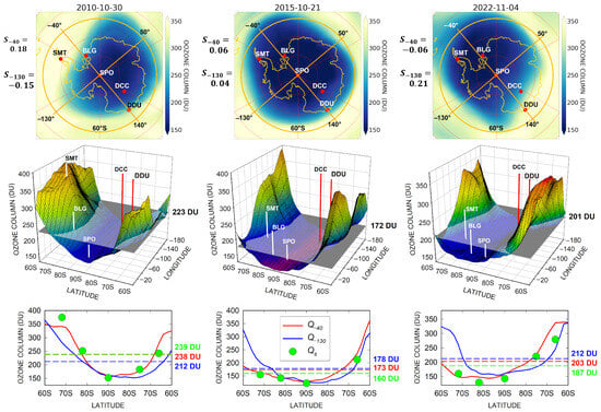
Figure 3.
Examples of the distribution of ozone columns in zone , defined as the area between 60°S and 90°S for the three days given by the columns. The upper panel in each column exhibits a map constructed from the ERA5 dataset, where the 60°S circle together with the and lines are also given. The second panel shows a 3D plot of the ozone in . The grey surface represents the level of the zonal average ozone and its amount is given on the right vertical axis. Five of the stations adopted in Section 2 are indicated through their GAW ID (see Table 1). The lower panel in each of the columns shows the latitudinal ozone patterns and in two sections of the corresponding 3D plot determined by (red curve) and (blue curve), respectively. In addition, the daily ozone amounts at the selected stations are also given by the green circles and ordered according to the station positions presented in the upper two panels. The average ozone amounts and calculated for the two curves and circles are indicated by the dashed lines, and the values are given on the right axis in the corresponding colors.
The meridional sections of the ozone distributions along and as functions of latitude are shown in the lower panels of Figure 3. The graphs suggest that the ozone column along and along smoothly and monotonously decrease from the initial point of the line at 60°S, reaching a minimum close to 90°S and smoothly and monotonously increase to the opposite end at 60°S. Such behavior keeps its character despite the significant day-to-day changes in the slope of the curves representing the longitudinal distribution of the ozone column. These changes are plausibly driven by the distortions and displacements of the polar vortex (and hence, the ozone hole) caused by planetary waves, which create appreciable differences in the ozone column measured at the exterior of the and strip stations. Nevertheless, looking at the graphs, a similarity in the broad outline among the curves can be noted. In this context, it can be assumed that the mean ozone columns and along and, respectively, should be close to each other. In fact, the values exhibited on the right of each panel show discrepancies of 12%, 3%, and 4% between and in the three cases. The zonal averages for the three days selected in Figure 3 are given in the middle row of panels on the right vertical axes. It can be seen that the difference between these averages, on the one hand, and the corresponding or on the other, varies from 1% to 7%. Hence, either or can be considered an approximation of the ozone column averaged over . Furthermore, the quasi-even geographical distribution of the stations result in the assumption that their mean ozone columns are able to represent and, in turn, the zonal average ozone column . Additionally, the mean ozone of the stations’ values given in the lower panels of Figure 3 show a discrepancy of about 8% regarding the corresponding values in the panels of the middle row. Thus, the examples given in Figure 3 indicate the possibility of gaining an approximate estimate of the average zonal ozone column by using ground-based instruments.
The cases examined in Figure 3 suggest a regularity in ozone distribution in , which may result from the previously discussed pattern in the ozone hole. In addition, the selected examples imply a certain symmetry of the ozone column with respect to the South Pole along the two axes, which is more pronounced in as the lower panels in Figure 3 show. This occurrence assumes an extent of axial symmetry in the zonal distribution with respect to since and are mutually perpendicular. The oval shape of the ozone hole, together with regularity and axial zonal symmetry regarding , where the stations are approximately located, could explain the closeness between and in the discussed examples. On the other hand, previous studies reported zonal asymmetry in the ozone distribution of Antarctica due to the equatorward displacement of the ozone hole [29,48,50]. The next subsection deals with this issue in the context of the present analysis.
3.2. Symmetry in the Zonal Average Ozone Distributions
Zonal asymmetry was assessed [48,50] as the relative difference between the lowest and highest ozone columns measured over arcs along a certain parallel . Such arcs were found to be located on approximately opposing sides. Since the concept of the present study assumes a comparison of mean values, the symmetrical features were estimated in terms of ozone averages in zone defined by latitude , using the ERA5 dataset. To this end, the average daily ozone over half of the zone determined by and the arc from −40° to 140° longitudes in the anticlockwise direction (see Figure 1 and Figure 3) can be compared with the average ozone estimated for the other half, determined by the −40° and 140° arc but to clockwise direction. Analogously, the averages and are calculated regarding . It is considered that the relative differences between the two averages can be defined as follows:
where denotes either −40 or −130 and is the zonal average ozone column in . could act as a measure of the axial asymmetry in .
Figure 4 shows an example of and time patterns in the period from September to December over several years, which indicate variations mostly between −0.10 and 0.30 except for quite limited cases. It should be noted that the values of given on the left of the upper panels in Figure 3 pertain to this range. Grytsai et al. [48] reported a maximum asymmetry of 32% at 65°S, examining September–November ozone averages. Meanwhile, Ialongo et al. [50] obtained up to 50% asymmetry in the daily ozone at the same latitude during October, which is consistent with the few extremes of in Figure 4. The semi-zonal averages used to define the parameter (see Equation (7)) instead of the minimal and maximal ozone along a parallel were assumed to play a smoothing role in estimating the asymmetry, reducing its magnitude.
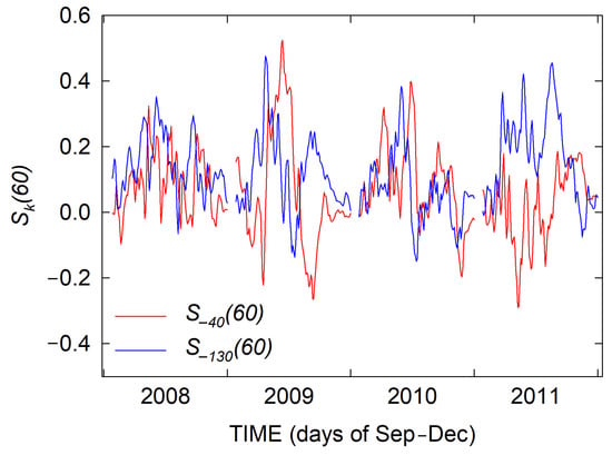
Figure 4.
Time patterns of and defined by Equation (7) and calculated for a 4-year period. The time for each year covers only the September–December period.
The relative distributions of and assessed for three different zones , and for each day of the studied period are given in Figure 5, together with the corresponding cumulative distribution functions (CDFs). The first two columns of Figure 5 show that the histograms of and differ from the Gaussian distribution. Thus, the conclusions about the statistical features of based on CDF in these two cases seem more reliable than estimating mean values (or medians) and standard deviations. It can be noted that the most probable values of and for 60°S and 70°S are very close to 0, but the right branches of the corresponding histograms are almost twice as long as the left ones. In fact, CDFs show that about 65% of and 80% of values are higher than 0. Table 2 gives the weights of three selected intervals in the distribution. It can be seen that the range contains about 75% of and , and 61% and 72% of and , respectively.
Table 2.
Percentages of values falling in the corresponding intervals.
The histograms of in Figure 5, both centered at about 0.035, are very close to the Gaussian distribution. In this case, the dispersion can be represented by the interval equal to (see Section 2). The lower asymmetry in the zone was also reported by Grytsai et al. [48] who estimated its value to be 10%. The high extent of symmetry in , expressed by almost equal and , presumed the quasi-uniform covering of the zone by the hole. The example presented in Figure 1 illustrates this conclusion. In fact, the area bounded by the 140 DU contour covered most of despite the fact that this area is slightly shifted equatorward in the longitudinal sector. The minimal ozone column on the considered in Figure 1 day was 126 DU. Hence, the discrepancy among the ozone amounts in the 140 DU area is about 10%, which assumes a quasi-uniform distribution. The increased asymmetry in the larger and zones could be a result of enhanced ozone fluctuations in the hole edges and the hole displacement.

Figure 5.
The upper two rows show the histograms of parameters calculated for the considered period (September–December of 2008–2022). The lowest row exhibits the corresponding cumulative distribution functions (CDFs) given in the same colors as the histograms. The mean values of with their standard deviations are given in the panels of the right column.
Figure 4 and Figure 5 show the prevailing weight of positive values in both and distributions that are more marked by and . This means that the average ozone column in the sector between −40°S and 140°S longitudes in the clockwise direction is lower than the average ozone in the other half of the zone, , according to Equation (7). Analogously, is predominantly true for the semizones obtained from the division of the zone by . These findings lead to the conclusion that in most cases of the Antarctic ozone hole in the last 15 years, the area of its minimal values tends to be displaced equatorward in the longitude sector. This result is consistent with those reported in [50] for the longitudinal sector where the zonal minimum of the 60°S circle is shifted. Grytsai et al. [48] found that the typical displacement of the ozone hole occurred towards the longitude quadrant .
Summarizing the results allows us to conclude that the cases with elevated levels of axial symmetry are predominant patterns in the zonal average ozone column. The percentages in Table 2 indicate that the extent of symmetry in terms of the average ozone columns in is higher with respect to than to . Bearing in mind the quasi-uniform ozone gradients to the hole center, the path of the hole shift could be considered an axis of symmetry in the zonal ozone distribution. Moreover, it was noted that approximately traces this path. In this context, the high zonal symmetry regarding seems explainable. Hence, the mean ozone amount along the axis of symmetry could act as an approximation of the average amount in the zone. On the other hand, the mean of the values measured at the stations on represent the axial ozone means according to the inference of the previous subsection. Thus, the axial symmetry and the quasi-uniform gradients appear to be important factors that enable the representation of the zonal average ozone column through the mean values of the ozone measured at stations along the axis of symmetry. A more detailed analysis of this issue, taking into account all the stations selected in Table 1 is the subject of the next section.
4. Results and Discussion
Figure 6 provides an example of the approximation of the zonal average ozone through ground-based measurements performed at two of the adopted stations in Table 1–DCC and BLG. The time patterns of the daily ozone columns and registered at DCC and BLG stations are presented in the lower panel of Figure 6 together with their mean values and the average calculated from ERA5 data for the and zones. It can be seen that the ozone columns measured at BLG and DCC were quite different from each other until the end of October. This can be accounted for by the different positions of the stations with respect to the ozone hole, as the upper panels of Figure 6 exhibit. Nevertheless, the mean is relatively close to both zonal average curves and , showing a different extent of closeness. In fact, the of the relative difference between and , estimated through Equation (6), is 10%, while it is 7% for the and relative differences. This enables an approximation of by . Hence, the chosen number of stations and their locations appear to be crucial factors for the area of the approximated zone. The next subsection examines this problem.
In the case of more than two stations, calculating the mean ozone column requires simultaneous measurements. However, maintaining this requirement is challenging for independent stations over long periods of time. In fact, the data gaps given in Table 1 suggest a possible lack of simultaneous observations in the case of a large number of stations. Table A1 shows that the ground-based measurements are predominantly inferior to the days in the ERA5 time series, which are 1830 for each sequence. This occurrence can result in a decline in the reliability of statistical conclusions. For that reason, the ERA5 dataset was used for the analysis in the next subsection, and Appendix A validates this replacement.

Figure 6.
The upper panels show the ozone distribution in Antarctica for four days of the austral spring in 2012 indicated by the panels. The positions of BLG and DCC stations are shown and and borders are indicated by the green and red circles, respectively. The lower panel gives time patterns of the daily ozone values and registered at BLG and DCC stations together with their mean and the average ozone determined for and from the ERA5 dataset. The vertical dashed lines indicate the days for which the ozone distribution is presented in the upper panels.
4.1. Approximation of the Average Ozone Column over Antarctica by the Mean of Station Values
To determine the zones , the daily ozone values at the points corresponding to the station’s positions were extracted from the gridded ERA5 data through bilinear interpolation. For tracking , nine station patterns of 2 to 10 stations were selected and are presented in Table 3. The first pattern contains the two stations used in the example in Figure 6. Both BLG and DCC are almost equally far off from the South Pole, and they pertain to the strip depicted by in Figure 1 and discussed in Section 3. The subsequent station patterns were constructed to cover gradually enlarging areas around the South Pole. The first six of them follow such a rule regarding stations on the path determined by . The seventh and eighth also include the Antarctic coastal stations in the longitudinal sector (see Figure 1), while the ninth pattern contains all the stations.
Table 3.
Station patterns composed by the stations given in the second column through the GAW ID from Table 1. The latitudes for which the median (see Section 4.2) of the ratio is closest to 1 are also given together with the corresponding , 10th and 90th percentiles, mean values, and standard deviations.
To quantify the aimed approximation, the ratio of the mean daily ozone column obtained from the values at the stations composing the pattern, and the average daily ozone evaluated for at time sampled in days, was calculated as follows:
where is the ozone column measured at the station of the pattern. Since the length of each time series simulated by the ERA5 dataset is determined by days for the period selected in Section 2, the length of time series must be the same for each and . Figure 7 presents an example of the behavior of three station patterns and different latitudes , while Figure 8 and Figure 9 exhibit a more general picture of the statistical properties discussed in the next subsection.
Systematic deviations of from one in all cases in Figure 7 can be noted for , and . A similar performance of can also be seen in Figure 6. In fact, the upper panels in Figure 6 show that the areas with low and high ozone values in are quite different for all the examined days. This means that their contributions to the zonal averages will be different since, for zonal averaging, the area turned out to be the weight. On the other hand, the panels show that one of the stations (BLG) is predominantly in the hole, while the other (DCC) is in the periphery within out of the hole in the area with high ozone values. The mean of these two stations’ ozone assumes the same weight as the low and high ozone values while the zonal average weights are different. The prevailing contribution of the high ozone area in leads to higher values of the zonal averages with respect to the stations’ means. Thus, the stations’ mean ozone underestimates the average zonal ozone in the cases presented in Figure 6. The systematic deviation of from one in Figure 7 suggests that such underestimation occurs frequently in the adopted period (2008–2020). However, the area with a high ozone column in (see Figure 6) seems to be much smaller than or comparable to the low ozone surface, which makes the zonal average close to the station means and, hence, centered close to one in the upper row of Figure 7.

Figure 7.
The upper row shows time patterns of the ratio for different and indicated in the panels and for all the years of the studied period. The medians (see Section 4.2) of the ratio calculated for each time series are also given. The yellow horizontal lines indicate . The lower row exhibits the histograms of for of the corresponding upper panels and , indicated in the histograms. The red vertical line in each of the lower panels represents the median , while the dashed and dotted lines give the 10th and 90th percentiles, respectively.
The systematic deviations discussed above are illustrated by the corresponding histograms shown in the lower panels of Figure 7 that exhibit a significant displacement of medians from one. On the contrary, the upper panels in Figure 7 and the histograms in the first column of Figure 9 indicate that the distributions of for 70°S, 68°S and 62°S are symmetrical and peak at one. Such symmetry is an important feature of the Gaussian distribution that assumes the median (also equal to the mean) as being the most probable value of the studied variable. In the cases of the zones determined by the medians are equal to one, which corresponds to the approximate equality of and as Equation (8) suggests. The next subsection is addressed to the existence and size of similar zones defined by latitude for all patterns, given in Table 3.
4.2. Determining the Zones
To ascertain the existence and determine the borders of the average ozone of which can be approximated by a given number of stations, the percentiles (see Section 2) of the ratios for any of the station patterns in Table 3 can be calculated using the station measurements extracted from the ERA5 data. Figure 8 shows the results of these calculations for varying between 56°S and 80°S. It can be seen that the medians reach values close to one at a certain latitude for each . Hence, for any of the patterns there exists a latitudinal zone for which the ozone column, determined as a mean of the values measured at the stations in is quite close to the zonal averaged amount. Figure 8 also shows that the 25–75th and 10–90th percentile intervals are narrowest at and the medians occupy almost the central part of the intervals. This circumstance supposes that the distribution of at is very close to the Gaussian one. At the same time, is gradually displaced from the intervals’ centers, as the histograms in Figure 7 confirm. The latitude together with and are given in Table 3 for each , while Figure 9 shows the histograms of for latitudes .

Figure 8.
Percentiles for the time series calculated for different station patterns as a function of latitudes . The lowest and upper borders of the rectangles indicate the 25th and 75th percentiles and respectively, while the horizontal lines in the rectangles denote the median . The lower and upper bars give the 10th and 90th percentiles and . The 5th and 95th percentiles and are indicated by the corresponding lower and upper triangles.

Figure 9.
Histograms of distributions for the considered station patterns and corresponding both indicated in panels. The red vertical line in each of the panels represents the median, while the dashed and dotted lines give the 10th and 90th percentiles, respectively.
As can be seen from Figure 9, distributions are similar to Gaussians since, according to the discussions in Section 2, the corresponding medians and mean values are equal to each other, as Table 3 confirms, and they mark the histograms’ peaks. This circumstance highlights the medians as the most probable values of the ratio at .
Table 3 shows that several station patterns give an acceptable approximation of the average ozone, making the station number reduction possible depending on the data availability. It should be pointed out that the fifth pattern in Table 3 was used to illustrate the subject of discussions in Section 3 (see Figure 3). The 10th–90th percentile intervals given in Table 3, containing 80% of the corresponding ratios , vary approximately between and for different . They slightly exceed the corresponding intervals (from to ), which include 68% of the ratios. Thus, it can be concluded that the error of the above approximations varies within 6–8%, assuming 10th–90th percentile intervals, or 5–7% assuming the use of the range. Figure 6 and Figure 10a show that the average zonal ozone column level in the deepest phase of the hole from September to October can vary from year to year within DU, approximately 35%. On the other hand, fluctuations from 30 DU to 100 DU () can be observed within this period. Thus, the accuracy of the discussed approximations enables the detection of the yearly changes for the average zonal ozone hole level and the typical ozone variability over a daily scale.
It is worth drawing a parallel between the above findings and the conclusions made by the authors of [59], who claimed that the ground-based data collected only at SPO can represent the ozone decline in the polar vortex during the winter.

Figure 10.
(a) Time patterns of the daily average ozone column for 2012 calculated over various determined by given in the graph. Panel (b) presents the analogous time patterns but for the ozone , which was also averaged over the considered years for each day with an increment of 2° between 56°S and 80°S.

Figure 11.
Histograms, similar to those in Figure 9, but for the dataset of the ground-based measurements. The station pattern , latitude and the number of the ratios are given in the panels. The red vertical line in each of the panels represents the median, while the dashed and dotted lines give the 10th and 90th percentiles, respectively.

Figure 12.
The upper row gives the ratio with its standard deviations for two years indicated in the panels. The number of observational days used to calculate the ratios is 93 in both cases. The second row presents the time patterns of the ozone columns and , their mean , and zonal means and for 1993 and 1997, respectively.
4.3. Deepness of the Ozone Deficit Assessed by the Zonal-Averaged Ozone Column
Since the ozone hole usually changes its shape and position from day to day, e.g., 60], it can be expected to have different representations of the hole’s deepness with diverse average ozone columns . In fact, the time patterns given in Figure 10a for various in 2012 confirm such an assumption. Figure 10b shows the curves of which are analogous to those in panel (a) but obtained through additional averaging over the 2008–2022 period for each day. Figure 10 indicates that both and gradually decrease with the increase in . It can be seen that the average ozone in bounded by the highest considered represents the deepest ozone depletion, which usually takes place in late September and early October. Also, bearing in mind the symmetry features in discussed in Section 3.2, it can be concluded that despite the displacement of the ozone hole to the longitudinal sector, the core of the hole is situated nearby the South Pole on average.
The results shown above should be taken into account when the average ozone column is approximated by ground-based measurements. Table 3 shows that station patterns one, two, and four provide approximations of the average ozone for the highest possible value of and these patterns will represent, to a higher extent, the depth of the ozone hole in the considered schemes, as Figure 10a confirms.
Significant short-period variability in zonal averages consistent with the findings yielded in [60] can be noted in Figure 10a. These variations are plausibly attributed to the dynamic processes impacting the ozone hole. The amounts presented in Figure 10b show good consistency with the ozone columns assessed in [34] for the 2008–2022 period.
4.4. Estimation of the Ratios Using the Available Ground-Based Dataset
The approach adopted in Section 4.2 was also applied to the available ground-based measurements. The results are presented through the histograms of in Figure 11. The ratios yielded from the ground-based measurements exhibit distributions similar to those in Figure 9. The histograms are slightly larger, possibly due to the much smaller number of ratios which is a consequence of the limited simultaneous observations at stations of the patterns given in Table 3. In fact, while the number of ratios in Figure 8 and Figure 9 is 1380, the corresponding is significantly lower in the presented in Figure 11 cases. Nevertheless, the histograms are shown close to the Gaussian distribution of with medians approximately equal to one. It should be noted that the histograms of for the last three station patterns in Table 3 are not presented in Figure 11 due to a number lower than 20 for the estimated ratios.
The results obtained were tested for repeatability by applying the considered approach to the data collected for two years—1993 and 1997—before the adopted period in Section 2. They were chosen, taking into account available data, and station pattern two (see Table 3) was the only one to be tested. The upper row of Figure 12 presents the ratio calculated for the selected years. As can be noted is near to one for and 72°S in 1993. Such an occurrence in 1997 appears for . The second row in Figure 12 shows the time patterns of ozone columns and observed at BLG and ARH during the two years along with their means and the zonal means , similarly to Figure 6. It can be seen that the curves closely represent the behavior of the corresponding with the RMS of relative differences (see Equation (6)) equal to 9% and 8% for 1993 and 1997, respectively. Hence, the conclusion that the mean ozone column over the zones determined by latitudes higher than 68°S–70°S can be approximated by the mean of values measured at two stations, is able to be extended behind the period adopted for the analyses.
4.5. Reconstruction of the Ozone Hole Position and Shape from Ground-Based Measurements
Section 3 highlighted ozone hole patterns characterized by quasi-uniform ozone gradients leading to a monotone increase in the ozone column from the central hole area to its edges. These features are an oval shape with a continuous and smooth contour tracing the points with 220 DU. Thus, it can be assumed that the position and shape of the ozone hole can be schematically reconstructed from the ozone columns determined at a few scattered Antarctic locations. To perform such a reconstruction using the station dataset, it should be taken into account that seven of the selected stations given in Figure 1 and Table 1 lie on the strip determined by . According to Section 3.2, this line, representing an axis of elevated symmetry in the average ozone over Antarctica, provides a section of the ozone hole (see Figure 3), which can be represented by ground-based measurements. In addition, the other three stations placed in the longitudinal sector could contribute to the better localization of the hole position.
Bearing in mind the above considerations, Figure 13 shows an example of a hole reconstruction for three days in 2010, for which data are provided for eight stations. The first row in Figure 13 shows the ozone columns at the stations projected on similarly to the lowest panels in Figure 3. Since SYO is far from , the values at this station in the upper row in Figure 13 are schematically presented with respect to SPO, depending on the SYO ozone column. The upper panels in Figure 13b,c show that the ozone minima were measured at SPO, which gives an idea about the hole center. In the case presented in column (b), it can be noted that BLG, SPO, ARH, DCC, and DDU are in the zone with DU. On the other hand, SYO and DDU, which are almost equally far from the central SPO station with about 100° angular elongations to each other, show quite similar ozone amounts close to 220 DU. This means these stations should be on the hole edges. The ozone column at MBI and SMT is relatively high, and since at BLG it is low, it can be concluded that the edge of the ozone hole should pass between BLG and SMT. These features show a circle-like shape in the ozone hole, centered at SPO in the middle panel of Figure 13b, indicated by the blue zone.
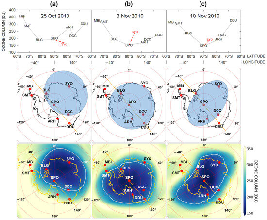
Figure 13.
The upper row shows the distributions of daily ozone columns for three days in 2010 along . The days are indicated in the upper panels of the (a–c) columns. The ozone column measured at SYO is also given, arbitrarily denoting the geographical position of the station in the graphs. The second row represents reconstructions of the ozone hole from the ground-based measurements shown by the blue areas. The third row exhibits the ozone hole for the selected days, reconstructed from the ERA5 dataset and outlined by the white curve.
Figure 13c gives another example of the ozone hole centered at SPO. However, in this case, the zone with DU projected on seems quite thin. Except for SPO, BLG, ARH, and DCC, which lie on , SYO also shows ozone values lower than 220 DU. Since both SPO–DCC and SPO–BLG distances are almost twice as small as the distance between SPO and SYO, the ozone hole, in this case, should have an elliptical shape with a major axis along the SPO–SYO direction as the middle panel of Figure 13c shows.
The upper graph in Figure 13a exhibits a case where the ozone minimum is displaced towards SYO, and only at BLG, SPO, DCC, and SYO is the ozone column less than 220 DU. In this case, the arc depicted by BLG, SPO, and DCC can be assumed to outline the edges of the ozone hole. Accordingly, the shape and position of the hole can be presented by the blue ellipse in the middle panel in Figure 13a, showing a displacement to the 0°–120° longitudinal sector.
The lower panels of columns (a), (b), and (c) in Figure 13 show the real shapes and positions of the ozone hole in the above cases represented by the ERA5 dataset. Generally speaking, a closeness between the reconstructed and observed holes can be noted regarding the shapes, centers, and covered areas. Due to the limited information provided by only eight stations, the reconstructed ozone holes can be depicted just through regular figures like circles and ellipses. Nevertheless, these images could provide preliminary information about the areas of strong ozone depletion over Antarctica in near-real-time.
This subsection presents some examples of the qualitative reconstruction of the ozone hole position and shape using ground-based measurements. The edges of the hole were drawn among the stations following an approximate approach that takes into account the ozone column measured at them. The development and usage of a more rigorous quantitative methodology to perform such a reconstruction is beyond the frames of the present study.
4.6. A Possible Contribution of Ground-Based Measurements to Studying Short-Term Pulsations in the Ozone Hole
All the above considerations concern the daily mean ozone columns. In fact, the ground-based measurements are able to represent short-time ozone variations within an hourly timescale that could describe the diurnal fluctuations of the ozone hole shape [60,61,62]. Figure 14 represents some examples of the ozone variations registered at four stations where measurements with high frequencies are available. The results are given in Figure 14 by red circles. It should be noted that the measurements at DCC and SPO were carried out with a nearly five-minute frequency, while at BLG and SMT, the time step was about 9 and 12 min, respectively. The hourly data taken from the ERA5 database are also shown in Figure 14 for comparison. Despite the general consistency between the two groups of time series in the left column of Figure 14, the ground-based measurements reveal stronger short-period dynamics in the ozone column presented by variations in DU. This occurrence is better seen in the right column of Figure 14, which shows the higher amplitude of the ozone variations found from the ground-based observations than those presented by ERA5 data. For instance, the variations in the period 1–2 November at BLG are almost twice as intensive as those represented by ERA5. A similar occurrence can be noted between 9 and 10 November at SMT and between 6 and 7 November at SPO. The latter case, presenting variations in more than 20 DU in the ozone column within a few hours, is consistent with the variations reported in [62].
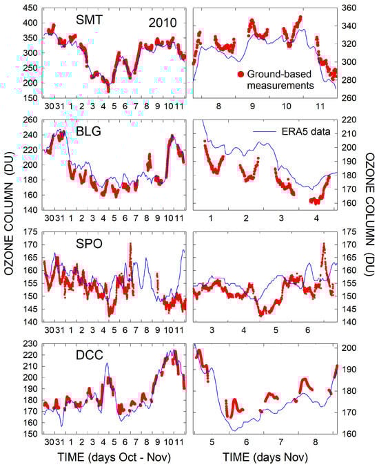
Figure 14.
Short-term variations in the ozone column presented through both ground-based observations (red circles) performed at 4 Antarctic stations indicated in the corresponding left panels and the ERA5 dataset (blue curve).
It is believed that similar results could contribute to the study of short-term pulsations in the ozone hole and, thus, the development of stratospheric dynamics on an hourly timescale.
5. Conclusions
The behavior of the Antarctic ozone hole was examined by analyzing two datasets. The first one was composed of ground-based observations performed at 10 Antarctic stations for the months of September–December during the 2008–2022 period. The second dataset was extracted from the ERA5 database over a grid of in both the latitude and longitude directions for the same period. Seven of the ten selected stations turned out to lie along the strip approximately depicted by the line determined through the −40° and 140° meridians, which have path traces observed in the past decades to shift in the ozone hole. A brief analysis of the considered datasets revealed smoothly varying patterns with quasi-uniform gradients in the distribution of the ozone column within the hole. In other words, the ozone behavior within the hole was characterized by a gradual and quasi-homogeneous change from the center to the edges. Additionally, a certain axial symmetry in the ozone over zones represented by circular areas around the South Pole was observed, as evidenced by the notable similarity between the averages in the two semi-zones defined by . These features suggest the possibility of approximating the daily zonal average ozone using the daily mean of the ozone measurements taken at various stations within the zone. To examine this possibility, the ratios between the mean ozone column found from the stations’ data and the average ozone in zones defined by latitudes varying from 52°S to 80°S were calculated. To this end, nine patterns, composed from 2 to 10 stations, were adopted. It was found that each station’s pattern corresponded to a zone defined by a given latitude in the above interval, for which the zonal average ozone column could be approximated by the mean ozone derived from the stations’ measurements. The accuracy of this approximation was estimated to be 5–7% at 1 and 6–8% at the 10th–90th percentage levels. Furthermore, ground-based observations conducted at various sites across the Antarctic continent facilitated a schematic reconstruction of the ozone hole’s shape and position. The high frequency of these measurements provided an opportunity to study ozone variations in both the inner regions of the hole and its edges on an hourly timescale.
Generally, the quasi-homogeneous gradients in the ozone distribution within the Antarctic ozone hole enable the near-real-time depiction of its main spatial features and allow for the approximate assessment of the average ozone column in Antarctic zones using ground-based observations.
Author Contributions
Conceptualization B.H.P. and V.V.; methodology, B.H.P., V.V., P.D.C. and K.L.; data curation H.A.O., A.G., A.L., M.M, B.H.P., I.K. and I.L.C.; formal analysis, B.H.P. and K.L.; software, A.C. and G.V.; visualization, C.F., S.P. and G.V.; writing and editing, B.H.P., I.L.C., K.L., C.F., I.K., S.P. and A.C.; investigation, B.H.P., V.V, K.L., P.D.C., I.K. and A.G.; resources, V.V., P.D.C., H.A.O., A.L. and M.M. All authors have read and agreed to the published version of the manuscript.
Funding
The study was partially supported by the RadiCa Project PNRA18–00026 funded by the Italian National Research Program in Antarctica (PNRA). K.L. was supported by the Ministry of Education, Youth and Sports of the Czech Republic project (VAN 2024).
Data Availability Statement
ERA5 reanalysis data were downloaded from the website of the European Centre for Medium-range Weather Forecasts (ECMWF), ERA5 reanalysis, https://doi.org/10.24381/cds.adbb2d47 (registration required). Total ozone column data were taken from the World Ozone and Ultraviolet Data Centre (WOUDC) https://doi.org/10.14287/10000001.
Acknowledgments
The authors gratefully acknowledge the European Centre for Medium-Range Weather Forecasts (ECMWF) for providing the ERA5 data of ozone column. The authors also thank The World Ozone and Ultraviolet Radiation Data Centre (WOUDC), and all organizations responsible and providing WOUDC with the ground-based measurements for each of the stations used here. We thank anonymous reviewers for their constructive and valuable comments and the journal team for moving our manuscript to the publication phase.
Conflicts of Interest
Author Ivan Kostatinov was employed by the company Proambiente S.c.r.l. The remaining authors declare that the research was conducted in the absence of any commercial or financial relationships that could be construed as a potential conflict of interest.
Appendix A
To examine the possibility of using the ERA 5 data instead of ground-based measurements, the daily ozone columns measured at the stations were compared with the corresponding values yielded from the ERA5 dataset through bilinear interpolation. Figure A1 shows some examples of this comparison indicating good consistency between the two datasets. To quantify the closeness between the two datasets, the ratio of the ozone column measured at station at day and the corresponding ozone extracted from the ERA5 database for the same station and day were calculated. Further, was averaged over time to obtain the mean for each of the stations. Table A1 gives calculated for the adopted period in Section 2, together with the standard deviations. The proximity of to one with variations of about 5% indicates an acceptable closeness among the ground-based measurements and ERA-5 data. Hence, the ERA5 data could represent the stations’ ozone columns with acceptable accuracy.

Figure A1.
Comparison between the ozone column variations registered at three of the selected stations and corresponding ERA5 data (on the left). The right column shows the stations versus ERA5 plots with the corresponding regression lines, slope coefficients , intercepts and determination coefficients .
Table A1.
Mean discrepancies between the ground-based measurements and the corresponding ERA5 values represented by the ratio .
Table A1.
Mean discrepancies between the ground-based measurements and the corresponding ERA5 values represented by the ratio .
| Station | Number of Measurements | |
|---|---|---|
| PES | ||
| SYO | ||
| ZOS | ||
| DDU | ||
| ARH | ||
| DCC | ||
| SPO | ||
| BLG | ||
| SMT | ||
| MBI |
References
- Bojkov, R. International Ozone Commission: History and Activities, IAMAS Publication Series No. 2., Oberpfaffenhofen, Germany. 2012. Available online: https://www.iamas.org/wp-content/uploads/2019/06/IAMAS-PubSer-No2.pdf (accessed on 22 March 2024).
- Cornu, A. Sur la limite ultraviolette du spectre solaire. Compt. Rendus Acad. Sci. 1879, 88, 1101. [Google Scholar]
- Hartley, W.N. On the absorption spectrum of ozone. J. Chem. Soc. 1881, 39, 57. [Google Scholar] [CrossRef]
- Hartley, W.N. On the absorption of solar rays by atmospheric ozone. J. Chem. Soc. 1881, 39, 111. [Google Scholar] [CrossRef]
- Fabry, C.; Buisson, H. L’absorption de l’ultraviolet par l’ozone et la limite du spectre solaire. J. Phys. 1913, 3, 196–206. [Google Scholar]
- Fabry, C.; Buisson, H. Etude de l’extremite ultra-violette du spectre solaire. J. Phys. 1921, 2, 197–226. [Google Scholar] [CrossRef][Green Version]
- Dobson, G.M.B.; Harrison, D.N.; Lawrence, J. Observations of the amount of ozone in the earth’s atmosphere and its relation to other geophysical conditions. Part III Proc. R. Soc. Lond. 1929, A122, 456–486. [Google Scholar]
- Lindemann, F.A.; Dobson, G.M.B. A theory of Meteors, and the density and temperature of the outer atmosphere to which it leads. Proc. Roy. Soc. Lond. 1922, A102, 411–437. [Google Scholar]
- Chapman, S. A theory of upper atmospheric ozone. Mem. R. Meteorol. Soc. 1930, 3, 103–125. [Google Scholar]
- Brasseur, G.P.; Solomon, S. Aeronomy of the Middle Atmosphere, 5th ed.; Springer: Dordrecht, The Netherlands, 2005; pp. 443–531. [Google Scholar]
- Dobson, G.M.B. Forty years research on atmospheric ozone at Oxford–a history. Appl. Opt. 1968, 7, 387–405. [Google Scholar] [CrossRef]
- Brewer, A.W.; Kerr, J.B. Total ozone measurements in cloudy weather. Pure Appl. Geophys. 1973, 106–108, 928–937. [Google Scholar] [CrossRef]
- Kerr, J.B.; McElroy, C.T.; Olafson, R.A. Measurements of total ozone with the Brewer spectrophotometer. In Proceedings of the Quadrennial Ozone Symposium, Boulder, CO, USA, 4–9 August 1980; London, J., Ed.; National Center for Atmospheric Research: Boulder, CO, USA, 1981; pp. 74–79. [Google Scholar]
- Van Roozendael, M.; Peeters, P.; Roscoe, H.K.; De Backer, H.; Jones, A.E.; Bartlett, L.; Vaughan, G.; Goutail, F.; Pommereau, J.-P.; Kyro, E.; et al. Validation of ground-based visible measurements of total ozone by comparison with Dobson and Brewer spectrophotometers. J. Atmos. Chem. 1998, 29, 55–83. [Google Scholar] [CrossRef]
- Platt, U.; Perner, D. Direct Measurements of Atmospheric CH2O, HNO2, O3, NO2 and SO2 by Differential Optical Absorption in the Near UV. J. Geophys. Res. 1980, 85, 7453–7458. [Google Scholar] [CrossRef]
- Platt, U.; Stutz, J. Differential Optical Absorption Spectroscopy: Principles and Applications; Springer: Weinheim, Germany, 2008; p. 597. [Google Scholar]
- Pommereau, J.P.; Goutail, F. Ozone and NO2 ground-based measurements by visible spectrometry during Arctic winter and spring 1988. Geophys. Res. Lett. 1988, 15, 891–894. [Google Scholar] [CrossRef]
- Bortoli, D.; Ravegnani, F.; Giovanelli, G.; Petritoli, A.; Kostadinov, I. Stratospheric nitrogen dioxide in Antarctic region. In Proceedings of the Quadrennial Ozone Symposium, Kos, Greece, 1–8 June 2004; Zerefos, C.S., Ed.; University of Athens: Athina, Greece, 2004; pp. 940–941. [Google Scholar]
- Wang, Y.; Puķīte, J.; Wagner, T.; Donner, S.; Beirle, S.; Hilboll, A.; Vrekoussis, M.; Richter, A.; Apituley, A.; Piters, A.; et al. Vertical profiles of tropospheric ozone from MAX-DOAS measurements during the CINDI-2 campaign: Part 1—Development of a new retrieval algorithm. J. Geophys. Res. Atmos. 2018, 123, 10637–10670. [Google Scholar] [CrossRef]
- Pfeilsticker, K.; Bösch, H.; Burrows, J.; Butz, A.; Camy-Peyret, C.; Dorf, M.; Gerilowski, K.; Grunow, K.; Gurlit, W.; Naujokat, B.; et al. Balloon-borne DOAS measurements of SCIAMACHY level 1 and 2 products. In Proceedings of the 16th ESA Symposium on European Rocket and Balloon Programmes and Related Research, Sankt Gallen, Switzerland, 2–5 June 2003; Warmbein, B., Ed.; ESA Publications Division: Noordwijk, The Netherlands, 2003; pp. 427–432, ISBN 92-9092-840-9. [Google Scholar]
- Pfeilsticker, K.; Platt, U. Airborne measurements during the Arctic Stratospheric Experiment: Observation of O3 and NO2. Geophys. Res. Lett. 1994, 21, 1375–1378. [Google Scholar] [CrossRef]
- Giovanelli, G.; Bortoli, D.; Petritoli, A.; Castelli, E.; Kostadinov, I.; Ravegnani, F.; Redaelli, G.; Volk, C.M.; Cortesi, U.; Bianchini, G.; et al. Stratospheric minor gas distribution over the Antarctic Peninsula during the APE–GAIA campaign. Int. J. Remote Sens. 2005, 26, 3343–3360. [Google Scholar] [CrossRef]
- Kokhanovsky, A.A.; Rozanov, V.V. The uncertainties of satellite DOAS total ozone retrieval for a cloudy sky. Atmos. Res. 2008, 87, 27–36. [Google Scholar] [CrossRef]
- Qian, Y.; Luo, Y.; Zhou, H.; Yang, T.; Xi, L.; Si, F. First Retrieval of Total Ozone Columns from EMI-2 Using the DOAS Method. Remote Sens. 2023, 15, 1665. [Google Scholar] [CrossRef]
- Gelaro, R.; McCarty, W.; Suárez, M.J.; Todling, R.; Molod, A.; Takacs, L.; Randles, C.A.; Darmenov, A.; Bosilovich, M.G.; Reichle, R.; et al. The Modern-Era Retrospective Analysis for Research and Applications, Version 2 (MERRA-2). J. Clim. 2017, 30, 5419–5454. [Google Scholar] [CrossRef]
- Hersbach, H.; Bell, B.; Berrisford, P.; Hirahara, S.; Horányi, A.; Muñoz-Sabater, J.; Nicolas, J.; Peubey, C.; Radu, R.; Schepers, D.; et al. The ERA5 global reanalysis. Q. J. R. Meteorol. Soc. 2020, 146, 1999–2049. [Google Scholar] [CrossRef]
- Chubachi, S. Preliminary result of ozone observations at Syowa station from February 1982 to January 1983. Mem. Nati. Inst. Polar Res. Spec. Issue 1984, 34, 13–19. [Google Scholar]
- Farman, J.C.; Gardiner, B.G.; Shanklin, J.D. Large losses of total ozone in Antarctica reveals seasonal ClOx/NOx interactions. Nature 1985, 315, 207–210. [Google Scholar] [CrossRef]
- Crook, J.A.; Gillett, N.P.; Keeley, S.P.E. Sensitivity of Southern Hemisphere climate to zonal asymmetry in ozone. Geophys. Res. Lett. 2008, 35, L07806. [Google Scholar] [CrossRef]
- Bian, L.G.; Lin, Z.; Zheng, X.-D.; Ma, Y.-F.; Lu, L.-H. Trend of Antarctic ozone hole and its influencing factors. Adv. Clim. Chang. Res. 2012, 3, 68–75. [Google Scholar] [CrossRef]
- WMO. Scientific Assessment of Ozone Depletion: 2018, Global Ozone Research and Monitoring Project Report, No. 58; WMO: Geneva, Switzerland, 2018; Chapter 4. [Google Scholar]
- Sibira, E.E.; Radionov, V.F.; Rusina, E.N. Results of Long-term Observations of Total Ozone in Antarctica and over the Atlantic and Southern Oceans. Russ. Meteorol. Hydrol. 2020, 45, 161–168. [Google Scholar] [CrossRef]
- Hartmann, D.L. The Antarctic ozone hole and the pattern effect on climate sensitivity. Proc. Natl. Acad. Sci. USA 2022, 119, e2207889119. [Google Scholar] [CrossRef]
- Kessenich, H.E.; Seppälä, A.; Rodger, C.J. Potential drivers of the recent large Antarctic ozone holes. Nat. Commun. 2023, 14, 7259. [Google Scholar] [CrossRef]
- Zhu, L.; Wu, Z. Climatic influence of the Antarctic ozone hole on the East Asian winter precipitation. Clim. Atmos. Sci. 2024, 7, 184. [Google Scholar] [CrossRef]
- Park, H.; Heath, D.F. Nimbus 7 SBUV/TOMS Calibration for the Ozone Measurement. In Atmospheric Ozone; Zerefos, C.S., Ghazi, A., Eds.; Springer: Dordrecht, The Netherlands, 1985. [Google Scholar] [CrossRef]
- Fleig, A.J.; Bhartia, P.K.; Wellemeyer, C.G.; Silberstein, D.S. Seven years of total ozone from the TOMS instrument-A report on data quality. Geophys. Res. Lett. 1986, 13, 1355–1358. [Google Scholar] [CrossRef]
- Bracher, A.; Lamsal, L.N.; Weber, M.; Bramstedt, K.; Coldewey-Egbers, M.; Burrows, J.P. Global satellite validation of SCIAMACHY O3 columns with GOME WFDOAS. Atmos. Chem. Phys. 2005, 5, 2357–2368. [Google Scholar] [CrossRef]
- Levelt, P.F.; Van den Oord, G.H.J.; Dobber, M.R.; Malkki, A.; Visser, H.; de Vries, J. The ozone monitoring instrument. IEEE Trans. Geosci. Remote Sens. 2006, 44, 1093–1101. [Google Scholar] [CrossRef]
- Toth, G.; Hillger, D. A brief history of ozone-monitoring satellites and instruments. Orbit 2011, 91, 12–17. Available online: https://rammb.cira.colostate.edu/dev/hillger/pdf/A_brief_history_of_ozone-monitoring_satellites_and_instruments.pdf (accessed on 15 September 2024).
- Kramarova, N.A.; Nash, E.R.; Newman, P.A.; Bhartia, P.K.; McPeters, R.D.; Rault, D.F.; Seftor, C.J.; Xu, P.Q.; Labow, G.J. Measuring the Antarctic ozone hole with the new Ozone Mapping and Profiler Suite (OMPS). Atmos. Chem. Phys. 2014, 14, 2353–2361. [Google Scholar] [CrossRef]
- Kokhanovsky, A.; Gascoin, S.; Arnaud, L.; Picard, G. Retrieval of Snow Albedo and Total Ozone Column from Single-View MSI/S-2 Spectral Reflectance Measurements over Antarctica. Remote Sens. 2021, 13, 4404. [Google Scholar] [CrossRef]
- Kokhanovsky, A.A.; Brell, M.; Segl, K.; Bianchini, G.; Lanconelli, C.; Lupi, A.; Petkov, B.; Picard, G.; Arnaud, L.; Stone, R.S.; et al. First Retrievals of Surface and Atmospheric Properties Using EnMAP Measurements over Antarctica. Remote Sens. 2023, 15, 3042. [Google Scholar] [CrossRef]
- Molina, M.J.; Rowland, F.S. Stratospheric sink for chlorofluoromethanes: Chlorine atom catalysed destruction of ozone. Nature 1974, 249, 810–812. [Google Scholar] [CrossRef]
- Crutzen, P.J.; Arnold, F. Nitric acid cloud formation in the cold Antarctic stratosphere: A major cause for the springtime’ ozone hole. Nature 1986, 324, 651–655. [Google Scholar] [CrossRef]
- Rowland, F.S. Stratospheric ozone depletion. Phil. Trans. R. Soc. B 2006, 361, 769–790. [Google Scholar] [CrossRef]
- Paul, A.; Newman, P.A.; Kawa, S.R.; Nash, E.R. On the size of the Antarctic ozone hole. Geophys. Res. Lett. 2004, 31, L21104. [Google Scholar]
- Grytsai, A.V.; Evtushevsky, O.M.; Agapitov, O.V.; Klekociuk, A.R.; Milinevsky, G.P. Structure and long-term change in the zonal asymmetry in Antarctic total ozone during spring. Ann. Geophys. 2007, 25, 361–374. [Google Scholar] [CrossRef][Green Version]
- Evtushevsky, O.M.; Grytsai, A.V.; Klekociuk, A.R.; Milinevsky, G.P. Total ozone and tropopause zonal asymmetry during the Antarctic spring. J. Geophys. Res. 2008, 113, D00B06. [Google Scholar] [CrossRef]
- Ialongo, I.; Sofieva, V.; Kalakoski, N.; Tamminen, J.; Kyrölä, E. Ozone zonal asymmetry and planetary wave characterization during Antarctic spring. Atmos. Chem. Phys. 2012, 12, 2603–2614. [Google Scholar] [CrossRef]
- Grytsai, A.; Klekociuk, A.; Milinevsky4, G.; Evtushevsky, O.; Stone, K. Evolution of the eastward shift in the quasi-stationary minimum of the Antarctic total ozone column. Atmos. Chem. Phys. 2017, 17, 1741–1758. [Google Scholar] [CrossRef]
- Yu, R.; Reshetnyk, V.; Grytsai, A.; Milinevsky, G.; Evtushevsky, O.; Klekociuk, A.; Shi, Y. Current trends in the zonal distribution and asymmetry of ozone in Antarctica based on satellite measurements. Ukr. Antarct. J. 2024, 22, 24–39. [Google Scholar] [CrossRef]
- Manney, G.L.; Santee, M.L.; Rex, M.; Livesey, N.J.; Pitts, M.C.; Veefkind, P.; Nash, E.R.; Wohltmann, I.; Lehmann, R.; Froidevaux, L.; et al. Unprecedented arctic ozone loss in 2011. Nature 2011, 478, 469–475. [Google Scholar] [CrossRef]
- Petkov, B.H.; Vitale, V.; Di Carlo, P.; Drofa, O.; Mastrangelo, D.; Smedley, A.R.D.; Diémoz, H.; Siani, A.M.; Fountoulakis, I.; Webb, A.R.; et al. An unprecedented Arctic ozone depletion event during spring 2020 and its impacts across Europe. J. Geophys. Res. Atmos. 2023, 128, e2022JD037581. [Google Scholar] [CrossRef]
- WOUDC. World Ozone and Ultraviolet Data Centre. 2024. Available online: https://woudc.org (accessed on 1 March 2024).
- Petkov, B.; Vitale, V.; Tomasi, C.; Bonafé, U.; Scaglione, S.; Flori, D.; Santaguida, R.; Gausa, M.; Hansen, G.; Colombo, T. Narrow-band filter radiometer for ground-based measurements of global UV solar irradiance and total ozone. Appl. Opt. 2006, 45, 4383–4395. [Google Scholar] [CrossRef]
- ECMWF. European Centre for Medium-Range Weather Forecasts, ERA-5 Reanalyses [Registration Required]. 2024. Available online: https://cds.climate.copernicus.eu/datasets/reanalysis-era5-single-levels?tab=overview (accessed on 1 February 2024).
- Brandt, S. Statistical and Computational Methods in Data Analysis, 2nd ed.; North-Holland Publishing Company: Amsterdam, The Netherlands, 1970. [Google Scholar]
- Fioletov, V.; Zhao, X.; Abboud, I.; Brohart, M.; Ogyu, A.; Sit, R.; Lee, S.C.; Petropavlovskikh, I.; Miyagawa, K.; Johnson, B.J.; et al. Total ozone variability and trends over the South Pole during the wintertime. Atmos. Chem. Phys. 2023, 23, 12731–12751. [Google Scholar] [CrossRef]
- Čížková, K.; Láska, K.; Metelka, L.; Staněk, M. Assessment of spectral UV radiation at Marambio Base, Antarctic Peninsula. Atmos. Chem. Phys. 2023, 23, 4617–4636. [Google Scholar] [CrossRef]
- Orte, P.F.; Wolfram, E.; Salvador, J.; Mizuno, A.; Bègue, N.; Bencherif, H.; Bali, J.L.; D’Elia, R.; Pazmiño, A.; Godin-Beekmann, S.; et al. Analysis of a southern sub-polar short-term ozone variation event using a millimetre-wave radiometer. Ann. Geophys. 2019, 37, 613–629. [Google Scholar] [CrossRef]
- Nichol, S.E.; Valenti, C. Intercomparison of total ozone measured at low sun angles by the Brewer and Dobson spectrophotometers at Scott Base, Antarctica. Geophys. Res. Lett. 1993, 20, 2051–2054. [Google Scholar] [CrossRef]
Disclaimer/Publisher’s Note: The statements, opinions and data contained in all publications are solely those of the individual author(s) and contributor(s) and not of MDPI and/or the editor(s). MDPI and/or the editor(s) disclaim responsibility for any injury to people or property resulting from any ideas, methods, instructions or products referred to in the content. |
© 2025 by the authors. Licensee MDPI, Basel, Switzerland. This article is an open access article distributed under the terms and conditions of the Creative Commons Attribution (CC BY) license (https://creativecommons.org/licenses/by/4.0/).