Multi-Source and Multitemporal Urban and Rural Settlement Mapping Under Spatial Constraint: Qinghai–Tibetan Plateau Case Study

Abstract

Accurately extracting long-term urban and rural settlement (URS) information is crucial for studying urbanization processes and their impacts on the ecological environment. However, existing remote sensing extraction methods often rely on independent classification strategies for each period, leading to error accumulation and increased uncertainty in long-term sequence extraction. To address this, this study proposed a data/model-constrained dynamic extraction method for URS information and validated it using the Qinghai–Tibetan Plateau at five-year intervals from 1985 to 2020. The area of URS extracted by this method had a matching degree of 97.79% with the reference, with an average overall accuracy of 93.25% and a kappa of 0.89 for the 1985–2020 confusion matrix sample. The urban and rural settlement boundary (URSB) extracted by this method were more accurate than the Global Urban Boundary (GUB) dataset, particularly in spatial completeness and boundary detail. The results provide technical support for uncovering urban development patterns and their environmental impacts.

1. Introduction

Urban and rural settlements (URSs) are urban and rural agglomerations, which are areas of high concentration of human activities [1], and key indicators for monitoring the urbanization process and its ecological changes [2,3]. Rapid expansion of URSs may lead to biodiversity decline [4], intensification of the urban heat island effect [5], hydrological processes, and climate change [6,7]. Understanding the dynamics of URS expansion is essential to reveal the urbanization process and its impacts on ecosystems [8,9].

Currently, long time series remote sensing-based mapping of URSs usually adopts the method of independent classification of products in each period, such as FROM-GLC [10], NUACI [11], and GlobeLand30 [12]. These products are generally updated every 1 or 5 years. However, due to the classification error in the data itself, it was often inaccurate to directly compare URS products from different time periods and analyze land use changes through differences, and we cannot tell whether the detected changes were caused by real land use changes or by classification errors. Studies have indicated that, compared to land cover classification errors, the areas of actual land cover change are relatively small [13]. Meanwhile, the independent classification method ignores the intrinsic correlation between URSs, leading to the need for processing, such as the test of temporal and spatial consistency, before analysis [14].

Unlike traditional independent classification methods, methods based on spectral trajectory analysis are able to monitor land use change through dense time series remote sensing imagery. This method analyzed the trajectories of variables (such as band reflectance) in time series to detect breakpoint structures, thereby identifying areas of land use change [15]. The large amount of open data provided by optical sensors, such as Landsat, has facilitated the development of algorithms based on the detection of time series trajectory changes, and typical algorithms include LandTrendr [16,17], Continuous Change Detection and Classification (CCDC) [18], Vegetation Change Tracker (VCT) [19], and Break Detection for Additive Season and Trend (BFAST) [20]. Among them, the CCDC algorithm demonstrated significant potential in land use change detection. It has been widely applied in fields such as vegetation dynamics monitoring [21] and impervious surface expansion [8] and has become the official algorithm for land use classification according to the United States Geological Survey. In recent years, dynamic monitoring methods for URSs based on the CCDC algorithm have been widely developed [8,22]. These methods can primarily be divided into two categories: The first involves time series model fitting, where classification is performed by extracting the fitting coefficients and root mean square error (RMSE) of the bands as classification features. However, in cases where early Landsat observation data are relatively sparse, the model’s fitting coefficients may introduce significant errors, thereby affecting classification accuracy [23]. The second category is based on a classification approach, where the “start year” and “end year” results for URS are extracted, and stable areas (i.e., regions where land use types remain unchanged) are identified through overlay analysis. Pixel-by-pixel change detection is then performed for land use change areas, ultimately completing the mapping of URSs. However, classification errors in the start and end years can introduce uncertainty in stable areas, which in turn affects the final extraction results. This issue was particularly pronounced for periods with poor remote sensing image quality (e.g., before the year 2000) and limited availability of multi-source data for support [24]. Therefore, the current urgent problem was how to construct a dynamic monitoring method for URSs adapted to the complex surface conditions in order to accurately extract the change areas and, at the same time, effectively reduce the influence of time series model fitting errors and classification errors on the results.

This study aims to develop a long time series URS extraction method based on data/model constraints, using Landsat dense time series imagery as the data source. The approach integrates CCDC algorithms, breakpoint detection algorithms, and an optimized random forest classification model, with the reference year serving as spatial constraints. Leveraging the Google Earth Engine (GEE), this study conducts a validation of URSs and their boundaries on the Qinghai–Tibet Plateau at a 30 m spatial resolution for five-year intervals from 1985 to 2020.

2. Research Area and Data Introduction

2.1. Research Area

The Tibetan Plateau ranges from 25°59′30″N to 40°1′0″N and 67°40′37″E to 104°40′57″E, with an area of 3,083,400 km² and an average elevation of 4320 m. The Qinghai–Tibet Plateau within the territory of China covers an area of about 2,581,300 km², with an average elevation of about 4400 km, and mainly includes the provinces and regions of Qinghai, Tibet, Sichuan, Gansu, Yunnan, Xinjiang, and other provinces and regions, of which the main parts of Qinghai and Tibet are distributed within the plateau [25]. The area covered in this study is mainly concentrated within China (Figure 1). The Qinghai–Tibet Plateau, with its vast territory and complex topography, is the highest plateau in the world. With its unique natural regional patterns and diverse ecosystems, it serves as a vital ecological barrier for China and the world. However, the region is ecologically fragile and its ecosystems are extremely sensitive to human activities and climate change.

2.2. Data Introduction and Pre-Processing

2.2.1. Landsat Remote Sensing Data

The Landsat program is an Earth observation satellite program jointly initiated and managed by the United States Geological Survey (USGS) and the National Aeronautics and Space Administration (NASA), and nine satellites have been launched so far [26]. This study utilized data from the Landsat series, including Landsat 5, Landsat 7, and Landsat 8, with a spatial resolution of 30 m.

Due to the high cloud coverage over the Qinghai–Tibet Plateau throughout the year, obtaining high-quality single-temporal satellite imagery is highly challenging. Therefore, cloud filtering and image compositing processes are required for the raw imagery data to enhance data quality. Taking the preprocessing of 2020 imagery as an example, the process began with cloud filtering by selecting images with less than 20% cloud cover from the annual dataset. Subsequently, cloudy pixels were removed using the built-in cloud removal algorithm in the GEE. The number and availability of images for each pixel were then analyzed to ensure that effective pixels covered the entire Qinghai–Tibet Plateau (as shown in Figure 2). Image composition was carried out using the median compositing algorithm provided by the GEE, processing the 1476 cloud-filtered images to generate high-quality remote sensing imagery on an interannual scale.

2.2.2. Sentinel-1 SAR Data

The Sentinel-1A satellite has a core payload of a C-band Synthetic Aperture Radar (SAR) with all-weather, all-day observation capability, which is able to penetrate clouds and provide high-resolution surface information [27]. This study performed median compositing of all SAR data acquired during 2020 to generate an interannual SAR image. At the same time, radar features with VV and VH polarizations are extracted and resampled to 30 m for subsequent modeling. VV means transmitting vertically polarized radar waves and receiving vertically polarized echoes. VH means transmitting vertically polarized radar waves and receiving horizontally polarized echoes. The Sentinel dataset has been preprocessed by removing thermal noise, radiometric calibration, and terrain correction. In the GEE platform, the VV and VH bands were automatically resampled to 30 m for mapping by setting the spatial resolution and adopting the bicubic interpolation method.

2.2.3. Nighttime Light Remote Sensing Data

Nighttime light (NTL) data, acquired through remote sensing satellites, are used to characterize the nighttime illumination conditions of the Earth’s surface. These data are typically collected by optical or infrared sensors aboard satellites or other remote sensing platforms and have been widely used in fields such as socioeconomic activities [28], light pollution [29], and urban expansion [30]. The commonly used NTL datasets include data from the Defense Meteorological Satellite Program and the Visible Infrared Imaging Radiometer Suite. This study utilized a time series NTL dataset [31] derived from the fusion of the above two products as the mask dataset for the potential URSs on the Qinghai–Tibet Plateau. The records in NTL data are digital number (DN) values, ranging from 0 to 63, where higher values indicate greater light intensity.

The minimum DN value of 7 was set as the segmentation threshold for the NTL data in the Qinghai–Tibet Plateau region. Using this minimum DN value helps reduce omissions in rural areas. This means that any DN value in NTL data in the Qinghai–Tibet Plateau region is considered a potential area of urban and rural settlements. In ArcGIS10.8.1 software, areas with DN values greater than or equal to 7 were extracted, resulting in the identification of the potential URSs on the Qinghai–Tibet Plateau for 2020. As shown in Figure 3, the extracted area essentially covers both urban and rural settlements within the Qinghai–Tibet Plateau, including most rural areas.

2.2.4. Digital Elevation Model Data

The Digital Elevation Model (DEM) is a digital representation of the Earth’s surface topography, typically recorded in raster format, with each pixel representing an elevation value. In this study, the V001 DEM created by NASA was used to extract elevation and slope information with a spatial resolution of approximately 30 m [32]. In the GEE, these data can be called via ee.Image (“NASA/NASADEM_HGT/001”).

2.2.5. Sampling Data

The Qinghai–Tibet Plateau was divided into two categories: URSs and others; URSs were categorized into high- and low-reflectance URSs according to the level of surface reflectance, and others included land cover types such as vegetation, water bodies, bare land, ice, and snow. Samples were obtained from Landsat data and Google Earth high-resolution images through visual interpretation [33,34], including training and validation samples, and the sample points were to be distributed as randomly and uniformly as possible in the study area (Figure 4). Among them, the number of sampling points is 589 in 2020 and 571 in 2015 for USRs, and 1332 in 2020 and 1369 in 2015 for the Non-URSs. In the model training process, 70% of the sampling points were selected as the training set and 30% as the validation set to evaluate the model’s performance and accuracy.

2.2.6. Validation Data

In this study, the GURS (Global Urban and Rural Settlement) [35], GAIA (Global Artificial Impervious Area) [36], and GISD30 (Global 30 m Impervious Surface Dynamic Dataset) [37] impervious surface or urban and rural settlements datasets were used to validate the accuracy of urban and rural settlements; Google Earth high-resolution historical imagery and GUBs (Global Urban Boundaries) [38] were used to validate the accuracy of the boundaries.

2.2.7. Qinghai–Tibet Plateau Boundary

The vector boundary of the Qinghai–Tibet Plateau used in this study comes from the National Qinghai–Tibet Plateau Science Data Center, and the boundary is named TPBoundary_HF [39].

3. Methods

3.1. Methodology for Mapping URSs on the Qinghai–Tibet Plateau in 2020

In this study, based on the GEE platform, we extracted the URSs and URSBs at 30 m spatial resolution on the Qinghai–Tibet Plateau in 2020 by using the established optimal random forest classification model for URSs and the technique of optimizing URSBs [40]. The main process includes (1) constructing an optimal random forest model based on spectral, topographic, and radar polarization features, and realizing the extraction of URS (2) based on morphological and eight-neighborhood pixel statistic techniques, aggregating discontinuous URSs, and filling in the inner natural space of the city to achieve the purpose of optimizing the boundaries of URSs (the same boundary mapping method is applied to the rest of the years). Considering the complexity of the features on the Qinghai–Tibet Plateau, which is prone to the phenomenon of “same spectrum, different objects”, this study combined the NTL remote sensing data to differentiate the background area and reduce the classification error of URSs in the Qinghai–Tibet Plateau.

The selected URS features include spectral features, topographic features, and radar polarization features, and 24 feature covariates were constructed to participate in the random forest model modeling (

Table 1. Indicators of remote sensing features of URSs.

Types	Feature Name	Description of Features	Value Range
Topographic features	Elevation	Elevation	[85, 8214]
	Slope	Slope	[0, 90]
SAR polarization features	VV	Polarization features	[−50, 1]
	VH	Polarization features	[−50, 1]
Spectral features	B2	Blue band	[0, 1]
	B3	Green band	[0, 1]
	B4	Red band	[0, 1]
	B5	Near-infrared band	[0, 1]
	B6	Shortwave infrared1 band	[0, 1]
	B7	Shortwave infrared2 band	[0, 1]
	B10	Thermal Infrared 1 band	[149, 372]
	TCB [41]	Tasseled Cap Brightness characteristics	[0, 4]
	TCG [41]	Tasseled Cap Greenness characteristics	[−2.2, 1.4]
	TCW [41]	Tasseled Cap Wetness characteristics	[−2.2, 1.8]
	BRI [40]	$\mathrm{BRI}={\displaystyle \frac{\mathrm{B}6-\mathrm{B}2}{\mathrm{B}6+\mathrm{B}2}}$	[−1, 1]
	NDBI [42]	$\mathrm{NDBI}={\displaystyle \frac{\mathrm{B}6-\mathrm{B}5}{\mathrm{B}6+\mathrm{B}5}}$	[−1, 1]
	NDISI [43]	$\mathrm{NDISI}={\displaystyle \frac{\mathrm{B}10-(\frac{\mathrm{B}3-\mathrm{B}6}{\mathrm{B}3+\mathrm{B}6}+\mathrm{B}5+\mathrm{B}6)/3}{\mathrm{B}10+(\frac{\mathrm{B}3-\mathrm{B}6}{\mathrm{B}3+\mathrm{B}6}+\mathrm{B}5+\mathrm{B}6)/3}}$	[0, 2.5]
	ENDISI [44]	$\mathrm{ENDISI}={\displaystyle \frac{2\times \mathrm{B}2+\mathrm{B}7/2-(\mathrm{B}4+\mathrm{B}5+\mathrm{B}6)/3}{2\times \mathrm{B}2+\mathrm{B}7/2+(\mathrm{B}4+\mathrm{B}5+\mathrm{B}6)/3}}$	[−1, 1]
	IBI [45]	$\mathrm{IBI}={\displaystyle \frac{\mathrm{NDBI}-(\mathrm{SAVI}+\mathrm{MDNWI})/2}{\mathrm{NDBI}+(\mathrm{SAVI}+\mathrm{MDNWI})/2}}$ $\mathrm{SAVI}={\displaystyle \frac{(1+0.5)(\mathrm{B}5-\mathrm{B}4)}{0.5+\mathrm{B}5+\mathrm{B}4}}$	[−1, 1]
	MNDWI [46]	$\mathrm{MNDWI}={\displaystyle \frac{\mathrm{B}3-\mathrm{B}6}{\mathrm{B}3+\mathrm{B}6}}$	[−1, 1]
	NDVI [47]	$\mathrm{NDVI}={\displaystyle \frac{\mathrm{B}5-\mathrm{B}4}{\mathrm{B}5+\mathrm{B}4}}$	[−1, 1]
	EVI [48]	$\mathrm{EVI}={\displaystyle \frac{2.5\times (\mathrm{B}5-\mathrm{B}4)}{\mathrm{B}5+6\times \mathrm{B}4-7.5\times \mathrm{B}2+1}}$	[−1, 1]
	RVI [49]	$\mathrm{RVI}={\displaystyle \frac{\mathrm{B}5}{\mathrm{B}4}}$	[0, +∞]
	DVI [50]	$\mathrm{DVI}=\mathrm{B}5-\mathrm{B}4$	[−1, 1]

).

3.2. Mapping Methodology for URS Dynamics on the Qinghai–Tibet Plateau During 1985–2020

This study proposed a method for extracting URS spatiotemporal information based on a multi-source data/model constraint approach, with the reference year serving as a spatial constraint (Figure 5). The main steps included three parts: (1) Creating the Maximum URS Baseline: The optimal random forest classification method was used to create the maximum URS baseline, which served as the spatial constraint for the reference year. (2) Breakpoint Detection: The CCDC time series model and breakpoint detection algorithm were applied to calculate breakpoint areas within the spatial constraint for the years 1985–2020 on a pixel-by-pixel basis. (3) Extracted Expansion Areas: Using 2015 as an example, all breakpoint areas from 2015 to 2020 were extracted and named as potential expansion areas. Based on classification methods, the actual expansion areas were extracted, and the URSs for 2015 were updated.

3.2.1. Continuous Change Detection Algorithm

(1) Time Series Fitting Algorithm

The Continuous Change Detection and Classification (CCDC) time series model is an algorithm that uses dense satellite image time series to monitor land cover and land use changes [18]. Specifically, it fits a curve for each pixel using all the Landsat historical images accumulated for the same region and detects changes by comparing the model’s predicted values. The CCDC algorithm can detect intra-annual changes caused by environmental seasonal factors such as temperature and precipitation, interannual changes due to climate change or land degradation, and sudden changes triggered by events like deforestation and urban expansion. In this study, the CCDC time series model was applied to fit the Landsat images from 1985 to 2020 for the Qinghai–Tibet Plateau:

$$\widehat{\rho }{(i,x)}_{OLS}=a_{0,i}+a_{1,i}\cos \left({\displaystyle \frac{2\pi }{T}}x\right)+b_{1,i}\sin \left({\displaystyle \frac{2\pi }{T}}x\right)+c_{1,i}x\left\{{\tau }_{k-1}^{*}<x\le {\tau }_k^{*}\right\}$$

(1)

where $x$ is the Julian day, $i$ is the $i$th band, $T$ is the number of days in a year ($T$ = 365), $a_{0,i}$ is the overall value coefficient of the $i$th band, $a_{1,i}$,$b_{1,i}$ are the intra-annual coefficient of variation in the $i$th band, $c_{1,i}$ is the inter-annual coefficient of variation in the $i$th band, ${\tau }_k^{*}$ is the kth breakpoint, and $\widehat{\rho }{(i,x)}_{OLS}$ is the predicted value of the $i$th band at the Julian day $x$ based on the Ordinary Least Squares (OLS) fitting.

(2) Breakpoint detection algorithm

The basic idea of breakpoint detection based on the CCDC algorithm is to calculate the difference between the fitted predictions of the CCDC time series model and the true satellite observations and compare it with the root mean square error (RMSE). When this difference is greater than three times the RMSE of the model (Equation (2)), the land cover of the site is considered to have changed and is considered a breakpoint.

$${\displaystyle \frac{1}{k}}{\displaystyle \sum _{i=1}^k\frac{\left|\rho (i,x)-\widehat{\rho }{(i,x)}_{OLS}\right|}{3\times {RMSE}_i}}>1$$

(2)

where $i$ represents the $i$th band; $k$ represents the number of image bands; $x$ represents Julian day; ${RMSE}_i$ is the RMSE of the $i$th band; $\rho (i,x)$ represents the observed value of the $i$th band predicted at $x$ on the Julian day; and $\widehat{\rho }{(i,x)}_{OLS}$ represents the predicted value of the $i$th band at $x$ on the Julian day.

3.2.2. Establishment of Reference Year Spatial Constraints

Generally, urban land use/cover transitions from Non-URSs to URSs, and this process is irreversible in the short term [17,51,52]. Based on this assumption, the spatial expansion of cities is constrained by the spatial distribution of URSs in the final period. Spatial constraints not only improve computational efficiency but also reduce confusion between other land use types and URSs. Since this study considers 2020 as the final study period, the 2020 URS extraction results for the Qinghai–Tibet Plateau were used as the maximum baseline and spatial constraint. This means that the distribution of URSs in earlier years must fall within this range, and by extracting the areas that underwent expansion, the URSs of previous years can be deduced.

3.2.3. Identification of Potential Expansion Areas for URS

Based on the CCDC algorithm and the breakpoint detection algorithm, it is possible to detect all the areas and time information where land use type changes may occur and define the areas where land cover type changes may occur during the study time period as potential expansion areas:

$$R=\left\{i\mid B_i=1 \mathrm{and} T_i\in \left[T_a,T_b\right]\right\}$$

(3)

where $R$ is the set of all pixels that satisfy the conditional breakpoints; $B_i$ represents the occurrence of breakpoints for the $i$th pixel, $B_i = 1$ means that a breakpoint is detected, and $B_i$ ≠ 1 means that a breakpoint is not detected; $T_i$ represents the time at which a breakpoint is detected for the ith pixel; $T_a$ and $T_b$ represent the beginning and the end of the study period.

All the above calculations were implemented on Google Earth Engine (GEE), and the specific parameters of the CCDC algorithm are shown in

Table 2. CCDC algorithm parameter settings.

Parameter Name	Type	Value
breakpointBands	List	GREEN, RED, NIR, SWIR1, SWIR2
tmaskBands	List	GREEN, SWIR2
minObservations	Integer	6
chiSquareProbability	Float	0.99
minNumOfYearsScaler	Float	1.33
DateFormat	Integer	1
lambda	Float	0.0022
maxIterations	Integer	10,000

. The GREEN, RED, NIR, SWIR1, and SWIR2 bands were selected for breakpoint detection. The dateFormat was set to 1, corresponding to fractional years, which makes interpretation easier. For example, changes detected in mid-2018 will be stored as 2018.5 in the pixel data. The lambda parameter was set to the default value of 20 and scaled to match the Landsat reflectance scale of 0.0022 [53].

3.2.4. Determination of Areas of Physical Expansion of URS

The potential expansion areas extracted using the above method undergo significant spectral changes during the corresponding time periods; however, such changes may not necessarily be caused by urban expansion. For example, activities such as urban renewal and new rural construction can also lead to abrupt spectral changes, which may erroneously be detected as breakpoint information, even though no actual urban expansion has occurred in that area. Therefore, further processing of the potential expansion areas is needed to obtain the actual expansion areas.

By referring to the random forest model built using 2020 as the reference year, an RF classification model based on spectral and topographic indexes was developed. The land use types in the potential expansion areas were classified into URSs and Non-URSs. In the classification results, the Non-URSs represent the actual expansion areas. Using 2020 as the high-precision reference year, subtracting the actual expansion areas yields the updated URS information for previous years. This method provides spatiotemporal dynamic information on URSs of the Qinghai–Tibet Plateau from 1985 to 2020.

3.3. Accuracy Evaluation

To evaluate the effectiveness and extraction accuracy of the method, this study conducted accuracy assessments from the following three aspects:

(1) Area Matching Accuracy.

Area matching accuracy refers to the degree of area match between two raster datasets. In this study, 2015 was used as an example, and URSs on the Qinghai–Tibet Plateau were extracted using two methods: the “Optimal Random Forest Algorithm Based on Multi-source Data” and the method proposed in this study. The extraction results from the “Optimal Random Forest Algorithm Based on Multi-source Data” were taken as the ground truth for the 2015 URSs on the Qinghai–Tibet Plateau. The accuracy was verified by comparing the area matching between the two methods:

$$S={\displaystyle \frac{S_1}{S_2}}\times 100\%$$

(4)

where $S$ represent the degree of area matching; $S_1$ represent the area of URS obtained using the method of this study; and $S_2$ represent the area of URS obtained using the optimal random forest model classification. The closer is to 100%, the more excellent the extraction results are.

(2) Confusion Matrix Accuracy Validation.

The accuracy metrics of the confusion matrix were calculated based on the GEE platform to evaluate the model’s accuracy. These metrics include overall accuracy, kappa coefficient, producer accuracy, and user accuracy [54]. Using the random sampling strategy, 30% of the samples were randomly selected as validation samples to assess the accuracy of URS extraction in 2020; at the same time, 30% of the samples of the “Random Forest Classification Method” in 2015 were randomly selected for the validation of the results of the method of this study.

(3) Comparison with other products.

The URS results of this study were compared with GURS, GAIA, and GISD30 datasets to assess the accuracy of URS extraction; this study showed [40] that the GUB product performs better in terms of boundary integrity and boundary accuracy compared to previous products, so the URSB results were compared with the GUB product to validate the accuracy of extracted boundaries in this paper.

A validation sample was randomly generated from the results of the three products described above. Specific methods included (1) overlaying the three sets of URSs or impervious surface data and classifying areas identified as URS in all three datasets as high-confidence urban and rural settlement areas and areas identified as Non-URS in all three datasets as Non-URS areas. The GURS dataset does not contain data prior to 2000, so the time period sample references the GIAD and GAIA overlay region; (2) randomly generating 1000 positive and 1000 negative samples in high-confidence URS areas and Non-URS areas in each of the seven years (1985, 1990, 1995, 2000, 2005, 2010, 2015, 2020) and constitute the validation sample; (3) calculating overall precision and kappa coefficients based on the confusion matrix of the validation sample of the year to assess the accuracy of the results of this study.

4. Results

4.1. Mapping of URSs and Their Boundaries on the Qinghai–Tibet Plateau in 2020

The importance score of each indicator for classification was assessed by combining spectral, topographic, and polarization features, the indicators were introduced gradually in ascending order of importance, and the overall accuracy of classification was calculated and plotted separately. The results showed (Figure 6) that the overall accuracy increased with the number of indicators introduced, reaching the highest value at the 11th indicator, and then the overall accuracy was maintained within a small fluctuation range of about 96% even when more indicators were added. Based on this analysis, the first 11 indicators were finally selected as classification features, including 7 spectral indicators, 2 topographic feature indicators, and 2 SAR feature indicators (

Table 3. Selection results after indicator optimization.

Feature Type	Initial Features Indicators	Optimized Feature Indicators
Spectral	B2-B7, B10, MNDWI, EVI, RVI, NDVI, DVI, ENDISI, BRI, NDBI, IBI, NDISI, TCB, TCG, TCW	B5, B10, ENDISI, BRI, NDBI, RVI, MNDWI
Topographic	slope, elevation	slope, elevation
SAR polarization	VH, VV	VH, VV
Total	24	11

).

Using the optimal random forest model and the urban and rural settlement boundary optimization extraction technique, a mapping of URSs and URSBs on the Qinghai–Tibet Plateau for 2020 was conducted (Figure 7). Since the details of URSs cannot be clearly displayed in the scale of the Qinghai–Tibet Plateau, eight typical cities are selected for display in this study, namely, Gar County of Ngari Prefecture, Shigatse, Lhasa, Nagqu, Golmud, Maqin County of Guoluo Tibetan Autonomous Prefecture, Xining, and Diqing Tibetan Autonomous Prefecture. The blue patches represent URSs, while the red boundary marks the URSBs. The results showed that the total area of URSs on the Qinghai–Tibet Plateau in 2020 was 2491.52 km², accounting for approximately 0.10% of the total area of the Qinghai–Tibet Plateau. The confusion matrix accuracy verification indicated that the overall accuracy was 97.15%, the kappa coefficient was 0.93, the producer accuracy was 94.61%, and the user accuracy was 95.75%. The classification performed well, with high accuracy, making it suitable as baseline data for subsequent studies. The generated boundaries effectively displayed the spatial extent of URSs for each city (Figure 7). These boundaries clearly distinguish URSs from surrounding land use types. Across different types of cities, whether dense or sparse, the boundaries exhibited good extraction results. For example, for larger cities such as Lhasa and Xining, as well as smaller cities like Gar County and Maqin County, the boundary extraction ensured the spatial connectivity of URSs. The extracted boundaries also encompass natural urban elements, such as water bodies and green spaces.

4.2. Mapping of URSs and Their Boundaries on the Qinghai–Tibet Plateau During 1985–2020

4.2.1. Potential Expansion Areas

Based on the potential expansion identification method, the time and frequency of breakpoints for all pixels within the spatial constraint were calculated pixel by pixel, and a spatiotemporal distribution model of breakpoint pixels from 1985 to 2020 was constructed. Potential expansion areas were extracted every five years, with eight typical cities selected for display (Figure 8). Due to the spatial constraint of the baseline range, background values were not included in the calculation and were displayed in black. The extracted URS areas clearly showcased regions where land cover type changes might have occurred during different time periods. For example, deep red areas represent regions where urban expansion may have occurred between 2015 and 2020. Based on the spatiotemporal variation in breakpoints, the spatiotemporal characteristics and trends of urban expansion from 1985 to 2020 can be indirectly represented.

4.2.2. Physical Expansion Areas

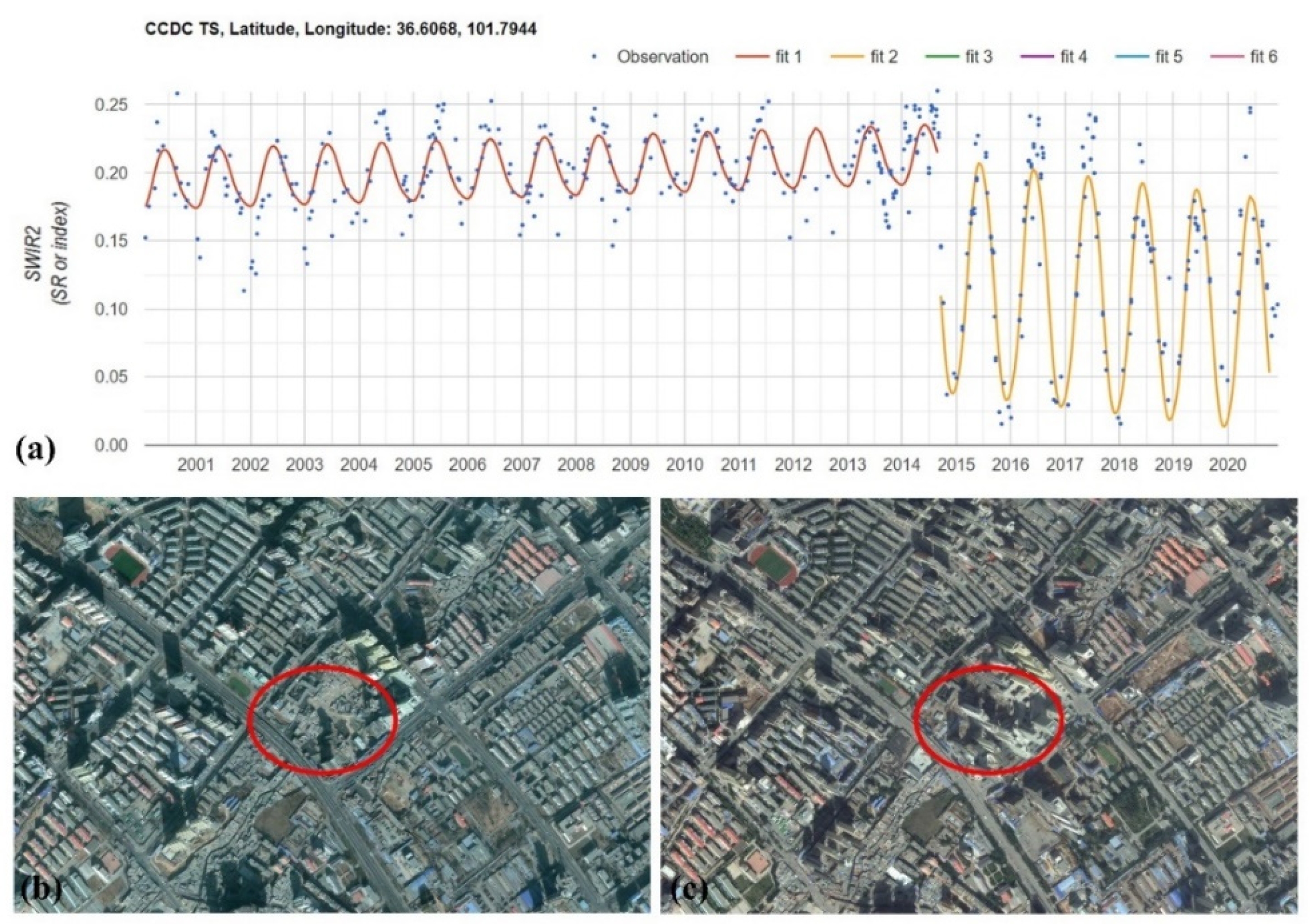
Urban demolition, reconstruction, and surface transformation activities can significantly alter the spectral characteristics of a region, leading to the detection of breakpoint areas. However, these changes do not necessarily indicate a change in land use types. Taking the urban renovation of a certain area as an example (Figure 9), from the high-resolution Google Earth imagery, it can be observed that in early 2014, the area was predominantly composed of low-rise residential buildings. By the end of 2015, high-rise buildings had been completed, indicating that the area underwent rapid building renewal within a short period. We can easily detect spectral abrupt changes through the CCDC algorithm and breakpoint detection algorithm. However, the update of buildings did not actually increase the area or extent of the city and should not be defined as urban expansion. Therefore, further identification of potential expansion areas is required.

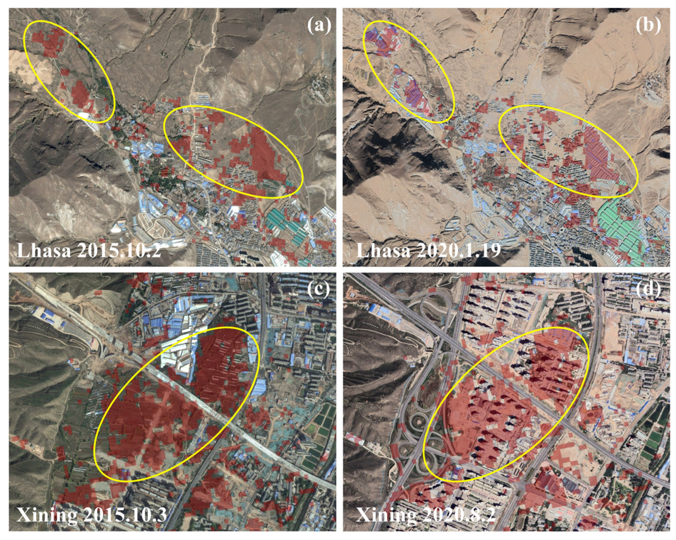
Based on the random forest classification model, the potential expansion areas were further classified to extract the actual expansion regions. The classification results for part of the potential expansion areas in Lhasa and Xining between 2015 and 2020 are shown (Figure 10). In the northwest of Lhasa’s Chengguan District, farmland (yellow area) was converted into URSs dominated by blue-roofed buildings between 2015 and 2020. Similarly, farmland in Xining (yellow area) was converted into URSs dominated by high-rise buildings during the same period, indicating that the classification results accurately extracted the actual expansion areas between 2015 and 2020. According to the classification accuracy statistics (

Table 4. Extraction accuracy of the actual expansion area of the Qinghai–Tibet Plateau during 1985–2020.

Periods	Overall Accuracy	Kappa	Producer Accuracy	User Accuracy
1985–1990	0.86	0.80	0.86	0.93
1990–1995	0.91	0.81	0.88	0.96
1995–2000	0.95	0.89	0.87	1
2000–2005	0.97	0.95	0.95	1
2005–2010	0.91	0.82	0.93	0.93
2010–2015	0.93	0.86	0.94	0.94
2015–2020	0.96	0.92	0.97	0.95

), the overall accuracy between 2015 and 2020 reached 0.96, with a kappa coefficient of 0.92, indicating that the random forest model can accurately extract the actual changes within the potential expansion areas. Overall, for the seven time periods from 1985 to 2020, the overall accuracy exceeded 0.86, suggesting relatively high classification accuracy. The kappa values were all above 0.80, indicating that the classification results are generally reliable. In most time periods, both producer and user accuracies remained high, demonstrating good recognition capability across all categories. The classification accuracy between 1985 and 1990 was lower compared to other years, which could be attributed to the lower quality of Landsat imagery from 1985. In conclusion, the random forest classification model can accurately extract actual expansion areas.

4.2.3. Update of URSs and Their Boundary Extraction

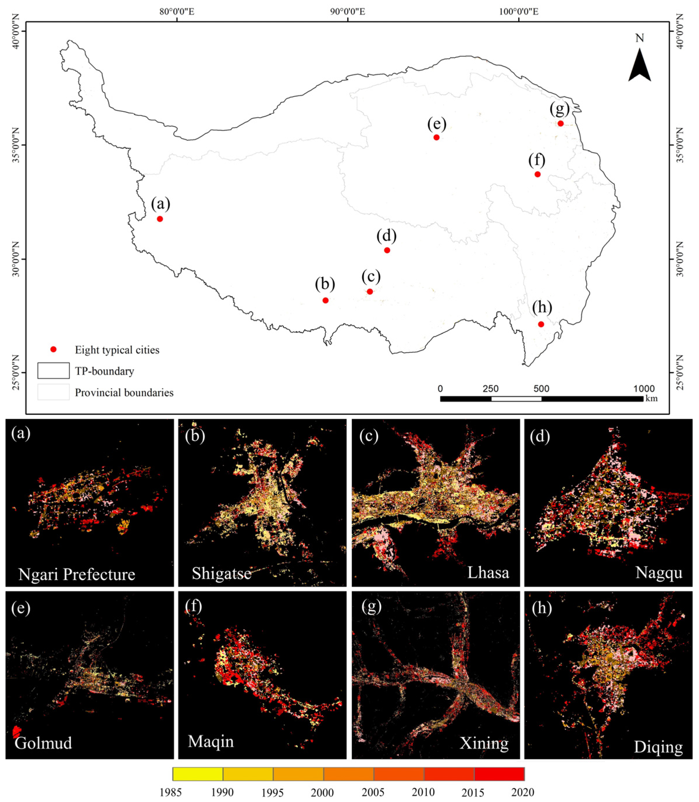
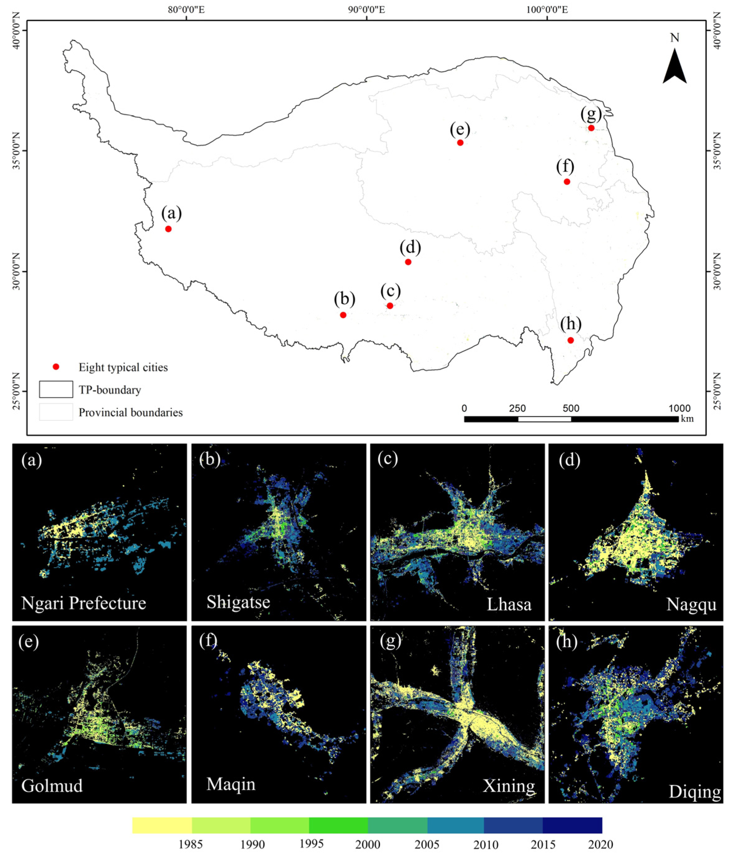
Based on the extraction results of the actual expansion areas, the URSs on the Qinghai–Tibet Plateau from 1985 to 2020 were updated (Figure 11), effectively reflecting the urbanization process over the past 35 years. Bright yellow and deep blue represent the spatial distribution of URS in the early 1980s and the late 2020s, respectively, and the gradient of colors shows the dynamic process of urban expansion. In 1985, URSs were mainly concentrated in city centers, after which rapid expansion began outward from the urban core. Particularly, in recent years, the acceleration of urbanization has led to more significant urban area growth. In the expanded areas, the blue tone dominates, indicating that most of the urban expansion occurred after 2010. For example, Lhasa expanded rapidly to the east and west after 2005, while Nagqu is relatively unique, with a smaller urban area and a dominance of yellow, indicating that the expansion of Nagqu has been relatively slow in recent decades.

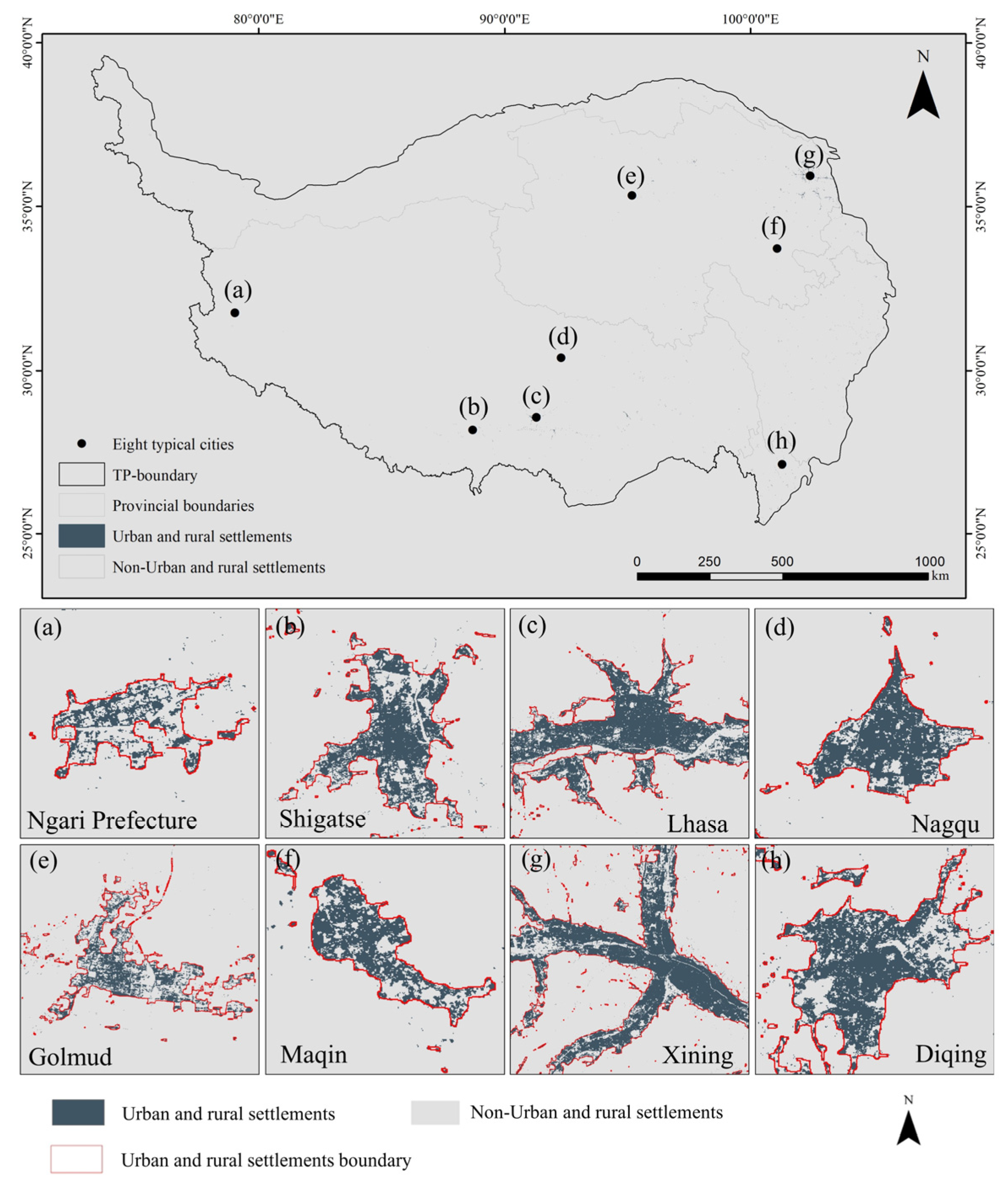
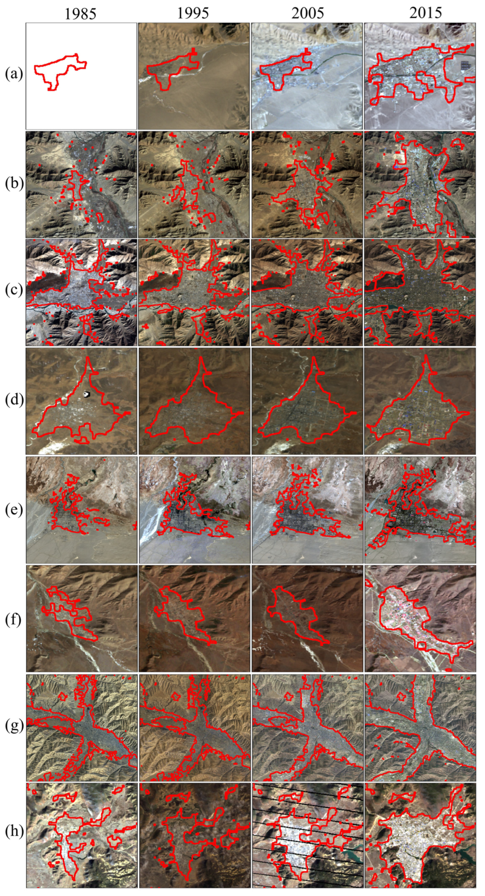
The URSBs were extracted based on mathematical morphology and pixel-based statistical methods, with an optimal morphological structural element radius of 13 [40]. Natural spatial features within the city were removed, and the URSBs on the Qinghai–Tibet Plateau from 1985 to 2020 were drawn and overlaid on Landsat satellite imagery. Figure 12 shows the boundary spatial patterns of eight typical cities, including Lhasa and Xining, for the years 1985, 1995, 2005, and 2015. The extracted boundary results closely align with the actual spatial extent of URSs, effectively separating URSs from other land use types, with continuous and complete boundaries. The migration of these boundaries reflects the urban expansion process, particularly between 2005 and 2015, where significant changes in boundary shape correspond to the rapid urbanization during that period.

4.2.4. Accuracy Evaluation

Based on the optimal RF classification model, the URS information of the Qinghai–Tibet Plateau for 2015 was extracted. A total of 1940 samples were used, with about 30% of the samples involved in accuracy validation. The random forest classification achieved an overall accuracy of 0.96, kappa value of 0.90, producer accuracy of 0.91, and user accuracy of 0.96, indicating high classification precision and reliable results, which can serve as baseline data.

(1) Area Matching Accuracy.

The closer the area matching S is to 100%, the higher the degree of matching and accuracy. The area matching accuracy for the entire Qinghai–Tibet Plateau, and eight representative regions such as Ngari Prefecture and Shigatse, was calculated (

Table 5. Area matching accuracy (area unit: km²).

Region	This Study	RF Model Method	Area Matching%
Qinghai–Tibet Plateau	2244.75	2295.55	97.79
Gar	5.29	5.24	101.09
Shigatse	64.53	77.02	83.79
Lhasa	155.21	162.66	95.42
Nagqu	22.22	21.36	104.01
Golmud	52.54	55.71	94.31
Maqin	8.09	7.63	106.03
Xining	351.66	329.15	106.84
Diqing	60.44	56.26	107.44

). The overall area matching accuracy for the Qinghai–Tibet Plateau reached 97.79%, indicating a high level of consistency between the datasets. The area matching degree for Shigatse was 83.79%, which may be due to errors caused by misclassification of bare soil in the random forest classification. For other cities, the area matching error was less than 8%, demonstrating relatively high matching accuracy at the city scale.

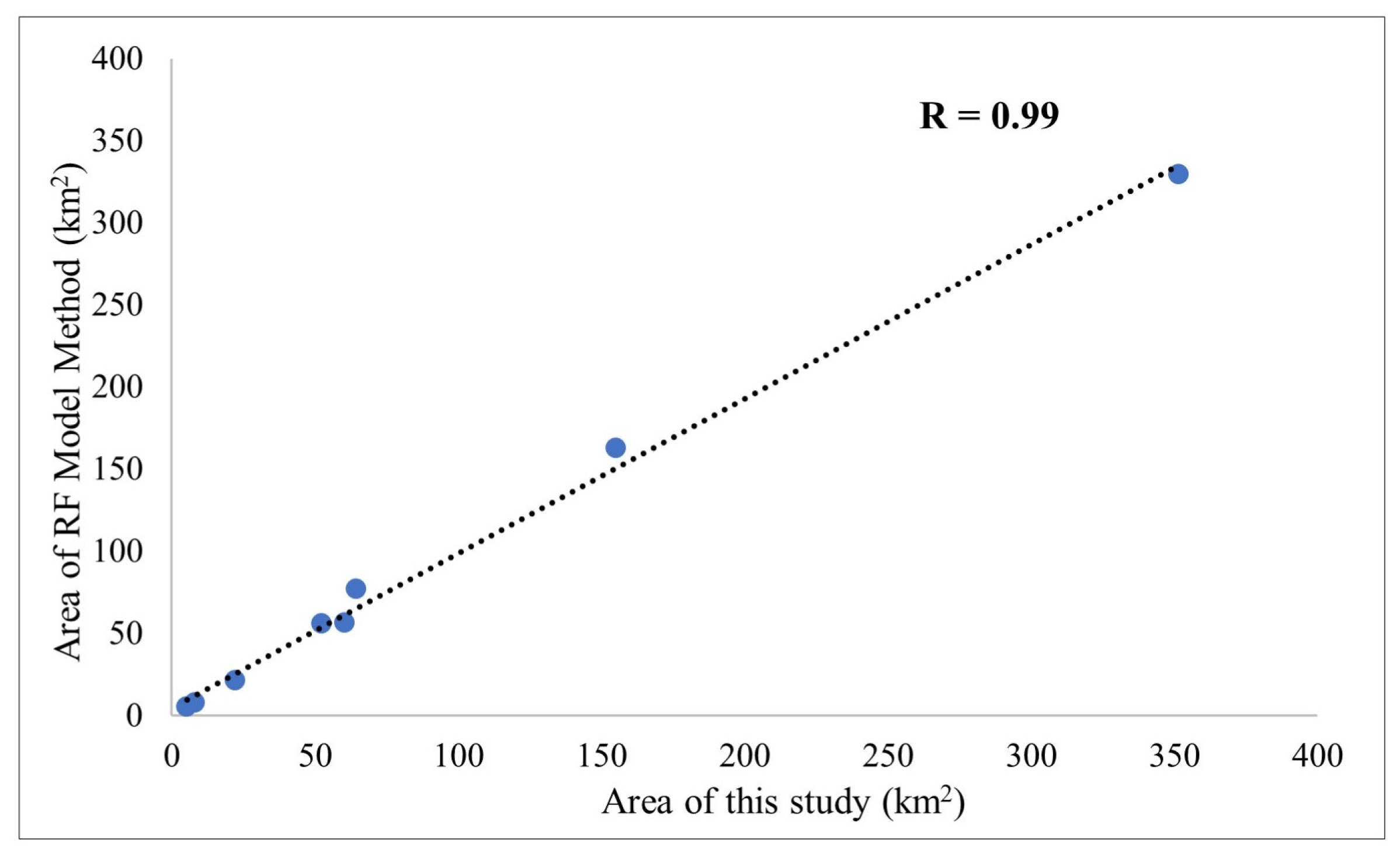
This study evaluated the accuracy of extracted areas through correlation analysis. Figure 13 presented a scatter plot with the areas extracted by this study’s method on the x-axis and those extracted by the “optimal random forest algorithm based on multi-source data” on the y-axis, including area data from eight typical cities. The results showed that the Pearson correlation coefficient between the two sets of data was as high as 0.99 (significance level p < 0.001), indicating a very strong correlation and consistency between the areas extracted by this study’s method and the reference areas, thus fully validating the accuracy and reliability of the method.

(2) Confusion Matrix Accuracy Validation

Based on the 1940 samples from the 2015 random forest classification, approximately 30% of the samples were randomly selected as validation samples to assess the accuracy of the URS extraction in this study. The results showed that the overall accuracy was 98.33%, with a kappa value of 0.96. For the “URS” class, the producer accuracy was 98.45%, and the user accuracy was 99.21%.

(3) Comparison with other products.

The validation sample of this study is based on the available GURS, GAIA, and GISD30 datasets, and the confusion matrix accuracy showed that the average overall accuracy of the URSs was 93.25% with a kappa coefficient of 0.89 (

Table 6. Accuracy of mapping URSs on the Tibetan Plateau from 1985 to 2020 based on a validation sample.

Year	OA (%)	Kappa
1985	89.76	0.85
1990	90.55	0.87
1995	91.86	0.87
2000	93.18	0.89
2005	94.65	0.90
2010	94.52	0.92
2015	95.81	0.93
2020	95.66	0.93
1985	89.76	0.85

). Specifically, in eight years (1985, 1990, 1995, 2000, 2005, 2010, 2015, and 2020), the overall accuracy is more than 90% and the kappa coefficient is more than 0.85. The overall presentation showed that the earlier the year, the lower the overall accuracy and the kappa coefficient, which may be due to the poor quality of Landsat imagery in the early years.

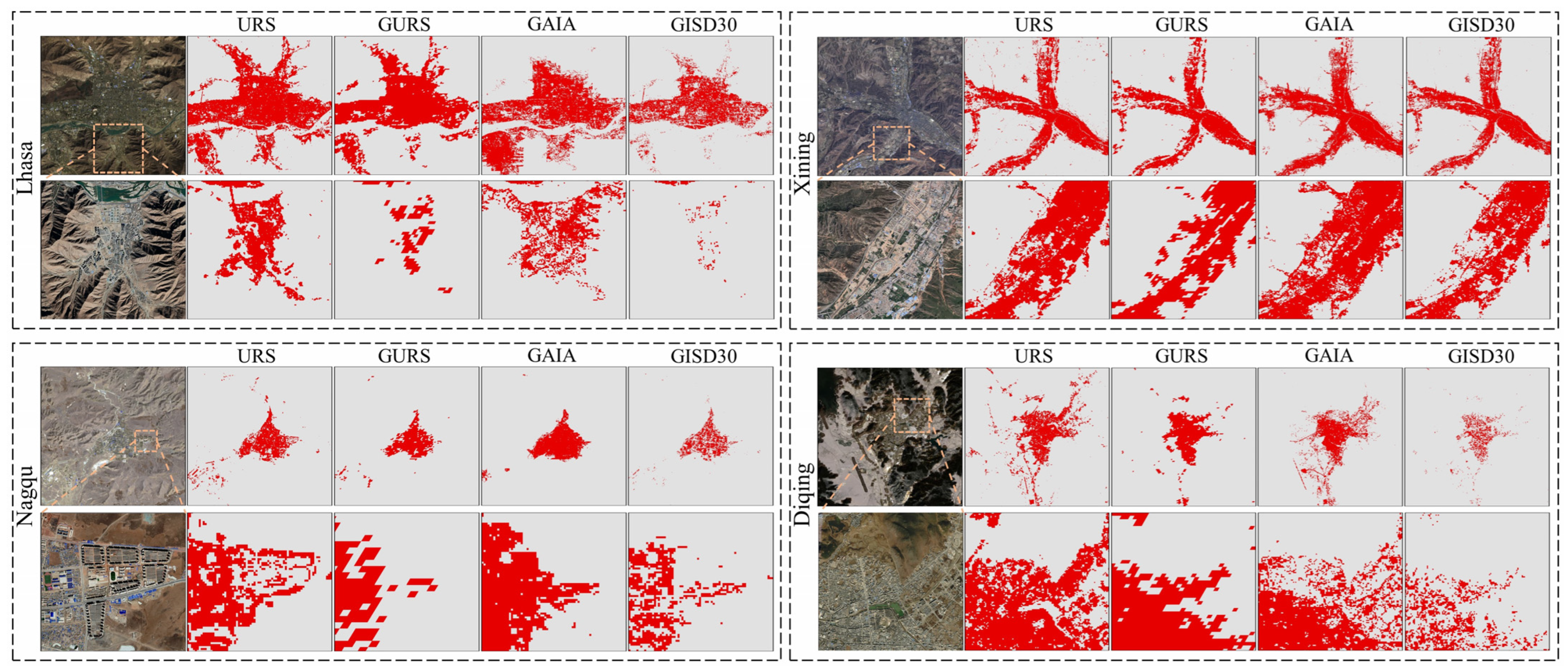
In addition to the quantitative evaluation described above, we selected four representative cities on the Tibetan Plateau (Lhasa, Xining, Nagqu, and Diqing Tibetan Autonomous Prefecture) to compare these datasets (Figure 14). The comparison reveals two main differences between URSs and other products. First, the ability to represent the spatial extent details of URSs was different. URSs have a high degree of consistency with the other products in terms of URSs in the urban subjects, and GURSs in particular exhibit a high degree of spatial accuracy. Due to the limitation of spatial resolution, GURSs (100 m resolution) have obvious jagged data, and the details of urban and rural settlements are slightly poorer. GAIA and GISD30 both have a spatial resolution of 30 m, but some rural settlements are missing, which makes the mapping ability weaker in rural areas. The ability of GURSs to show the details can more accurately reflect the dynamics of the urban sprawl. Second, the phenomenon of overestimation and underestimation of URSs. Taking Lhasa as an example, GURSs ignored low-density urban and rural settlements; GAIA misclassified bare land as URSs and overestimated the actual extent, which may be due to the fact that URSs have similar spectral characteristics to bare land and the classification process only considered the spectral characteristics of URS; GISD30 greatly underestimated URSs; and the product of the present study greatly mitigated the problem of misclassification and omission, and was in line with the actual situation maintain high consistency and high classification accuracy. The same phenomenon was found in other typical cities.

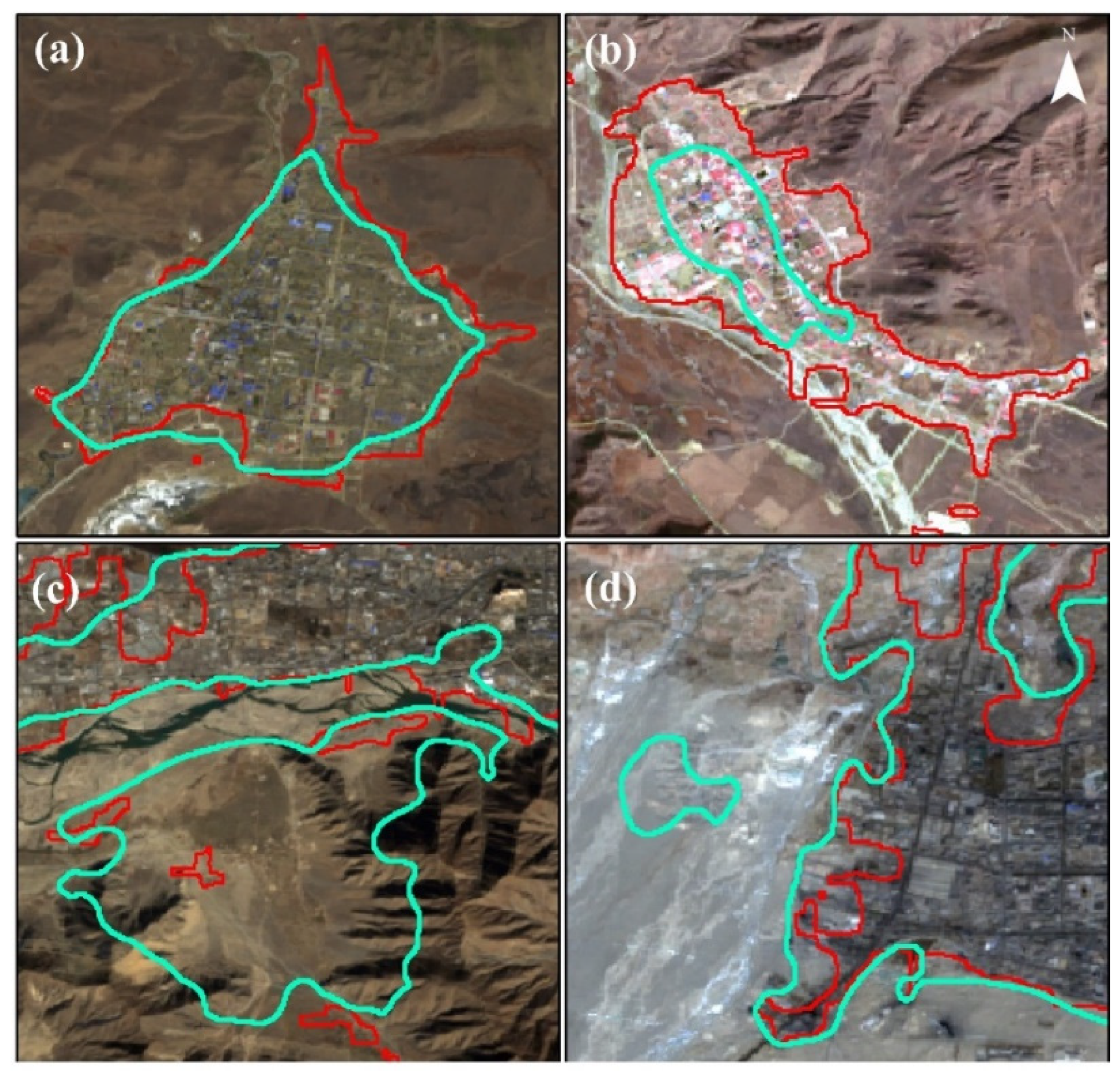
There are two main areas of difference between URSBs and GUBs in the comparison of urban and rural settlement boundaries (Figure 15). The first is the difference in the extent of the city. Although the extent in the core urban areas is highly consistent, the GUB product clearly overestimates or underestimates the urban boundaries to varying degrees. For example, in Figure 15a,b, the GUB underestimates the actual urban extent by overlooking the buildings in the surrounding areas. In Figure 15c, the southern part of Lhasa in 1995 had not been developed and was mainly covered by bare land and grassland, yet the GUB incorrectly extracted the urban range. The overestimation of the urban boundary may be due to the similar spectral characteristics of bare land and URSs. Figure 15d also showed an incorrect estimation of the urban boundary, as the western part of Golmud in 2005 was a river alluvial fan with no human habitation traces. URSB and URS product mapping ideas are similar; both are based on the secondary processing of urban and rural settlements to generate maps. That is, URSB is based on URS data, and GUB is based on GAIA products; however, GAIA products only consider spectral characterization indexes in the non-arid areas, so GUBs will be wrongly scored and omitted. Second, the level of detail of the boundaries was different. Both the URSB and the GUB datasets have a spatial resolution of 30 m. As shown in Figure 15a,b, the boundaries in this study effectively identify Non-URS areas, with the boundary shape being more irregular, while the GUBs were relatively smoother.

4.3. Changes in URS Area on the Qinghai–Tibet Plateau During 1985–2020

To accurately describe the temporal evolution characteristics of cities on the Qinghai–Tibet Plateau, the Expansion Velocity Index (V) is introduced. V refers to the change in the URS over a certain period and is one of the most fundamental indicators for studying urban expansion [55]:

$$V={\displaystyle \frac{S_b-S_a}{ T}}$$

(5)

where $V$ represents the rate of urban expansion in a certain period of time in km²/a; $T$ represents the time interval studied; and $S_b$ and $S_a$ represents the URS at the end of urban expansion (time $b$) and the beginning of urban expansion (time $a$), respectively. Calculate the area of URSs and their expansion rates in the Qinghai–Tibet Plateau region from 1985 to 2020 (

Table 7. Area of URSs on the Qinghai–Tibet Plateau during 1985–2020 (km²).

Year	Area (km2)	V (km2/a)
1985	1338.56	--
1990	1388.83	10.05
1995	1474.09	17.05
2000	1502.38	5.66
2005	1615.32	22.59
2010	1911.22	59.18
2015	2244.75	66.71
2020	2491.52	49.35

).

From 1985 to 2020, the URS area on the Qinghai–Tibet Plateau experienced significant changes. The URS area increased from 1338.56 km² in 1985 to 2491.52 km² in 2020, an increase of 1152.95 km², representing an overall growth of 1.86 times. From 1985 to 1995, the expansion velocity gradually increased. Although there was a slight decline during the 1995–2000 period, the overall trend remained upward. The period from 2005 to 2015 saw a significant increase in the expansion speed, especially between 2010 and 2015, when the expansion velocity grew rapidly, reaching its peak. From 2015 to 2020, although the expansion speed slowed down, it still remained at a relatively high level. Overall, during the entire study period, the expansion of URSs on the Qinghai–Tibet Plateau showed a trend of first increasing and then decreasing, with rapid growth in expansion speed particularly after 2005.

5. Discussion

5.1. Maximum Baseline Range Spatial Constraints

This study, based on the irreversible spatiotemporal pattern of URS expansion, utilized the maximum spatial constraint of the reference year and achieved good results. This constraint greatly improved computational efficiency in the spatial domain, reducing unnecessary workload. In the temporal domain, the method used the irreversible rule, treating the URSs at the end of the study period as spatial constraints. By calculating the pixels where Non-URSs were converted into URSs within a certain period, the spatiotemporal distribution of URSs in that year was indirectly derived. Compared to traditional post-processing operations that eliminate unreasonable land cover results, such as time consistency tests [56,57], this method avoided potential new errors that could be introduced by post-processing, improving the accuracy and reliability of the method. Additionally, the method established in this study effectively solved the issue of accumulated classification errors in the early stages of research. It optimized the process by requiring classification only for the “end year” rather than extracting URSs for both the “start year” and “end year”.

In most cases, the city limits at the end of the period will usually encompass the city limits according to the rule of irreversibility of urban expansion. This is because urban sprawl is usually characterized by a gradual process of outward expansion, and this expansion is generally irreversible, meaning that once urban areas have expanded to a certain place, these areas usually do not shrink back. In some exceptional cases, it is theoretically possible for areas to “break away” from city boundaries if they are degraded or altered (e.g., as a result of natural disasters, policy adjustments, land use changes, etc.), but this is usually rare.

5.2. Factors Affecting the Extraction Accuracy

(1) Nighttime lighting data.

In urban areas, the extracted potential urban extent is much larger than the actual urban area due to the light spillover effect of nighttime lighting data [58,59]; in rural areas, small and isolated rural settlements may lead to omissions due to limited sensor resolution [60]. Studies have shown that different nighttime light processing methods can lead to significant differences in nighttime light data products [61]. Therefore, it is necessary to try to use different sources of nighttime lighting data in future studies and explore their effects on the extraction results of urban and rural settlements.

(2) Type and number of indicators.

Studies have shown that the combination of multi-source data can significantly improve the accuracy of mapping urban and rural settlements [62]. The combination of spectral, topographic, and radar polarization features can reduce the confusion between bare rock, fallow land, and urban and rural settlements in high-altitude areas [40]. Optimizing the number of indicators can improve the efficiency and accuracy of random forest model classification and avoid the occurrence of “dimensionality disaster” [63]. Therefore, this study optimized the number of indicators from 24 to 11, including 7 spectral indices (B5, B10, ENDISI, BRI, NDBI, RVI, MNDWI), 2 topographic features (slope, elevation), and 2 radar polarization features (VV, VH).

(3) Low Data Frequency in the Early Stages of the Study

The accuracy of the CCDC algorithm in monitoring land use changes depends on the availability of Landsat observations. As the frequency of Landsat observations increases and more satellite imagery becomes available, the model’s fitting may have fewer biases [64], improving the algorithm’s accuracy [18]. In the 1980s and 1990s, the availability of Landsat observation data was limited, and the CCDC model was unable to accurately predict future observations, leading to errors in breakpoint detection [23]. This could contribute to potential errors in this study’s method.

(4) Breakpoint Detection Threshold Parameters

Studies have shown that a threshold of three times the RMSE is commonly used to detect breakpoints, but when the threshold is changed to two times the RMSE, finer land use changes can be detected [18]. Therefore, the setting of the breakpoint threshold can affect the final extraction results. Future research could analyze the impact of CCDC parameters on the results in more detail.

(5) Spectral Confusion

The URS extraction method based on the CCDC algorithm and random forest classification model has not completely resolved the issue of spectral confusion. The Qinghai–Tibet Plateau features a diverse and complex range of land cover types, with bare land and sandy areas sharing similar spectral characteristics with URSs. This similarity can lead to overestimation or underestimation of actual URS areas during classification, thereby affecting the accuracy of boundary extraction. Studies have shown that collecting more samples of bare land and urban areas can reduce this classification error [8]. Alternatively, using auxiliary datasets like population density and nighttime lights can help create urban masks for extracting urban areas, reducing interference from other land cover types [65]. The high heterogeneity of urban landscapes also leads to the widespread presence of mixed pixels, which further reduces the accuracy of change detection [24].

6. Conclusions

To achieve high-accuracy long-term extraction of urban and rural settlements and their boundary information, this study proposed a multi-source data/model-constrained extraction method. The findings demonstrated that spatial constraints based on high-accuracy reference year URS areas effectively excluded land cover types unrelated to urban expansion, reduced computational demand, and ensured logical consistency in urban expansion over time. By integrating the CCDC time series model, breakpoint detection algorithm, and random forest classification model, this method precisely calculated actual expansion areas and dynamically updated URS information for specified time points. The results showed that the area of URSs extracted by the method of this study had an area match of 97.79% with the area extracted by the optimal random forest classification method (2015 baseline area); the overall accuracy of the confusion matrix based on the validation of the sample set of multiple products was 93.25%, with a kappa coefficient of 0.89. Comparing the extracted URS boundary with the Global Urban Boundary (GUB) dataset revealed that the boundaries extracted using this method were closer to reality, with superior spatial accuracy and finer boundary details. Further analysis indicated that the area of URSs on the Qinghai–Tibet Plateau continuously expanded from 1338.56 km² in 1985 to 2491.52 km² in 2020, with the expansion rate showing a trend of initial acceleration followed by deceleration.

References

1. Zhang, J.; Feng, Z.; Jiang, L. Progress on studies of land use/land cover classification systems. Resour. Sci. 2011, 33, 1195–1203. (In Chinese) [Google Scholar]
2. Mudau, N.; Mwaniki, D.; Tsoeleng, L.; Mashalane, M.; Beguy, D.; Ndugwa, R. Assessment of SDG indicator 11.3.1 and urban growth trends of major and small cities in South Africa. Sustainability 2020, 12, 7063. [Google Scholar] [CrossRef]
3. Kaur, H.; Garg, P. Urban sustainability assessment tools: A review. J. Clean. Prod. 2019, 210, 146–158. [Google Scholar] [CrossRef]
4. Güneralp, B.; Seto, K. Futures of global urban expansion: Uncertainties and implications for biodiversity conservation. Environ. Res. Lett. 2013, 8, 014025. [Google Scholar] [CrossRef]
5. Jiang, S.; Peng, J.; Dong, J.; Cheng, X.; Dan, Y. Conceptual connotation and quantitative characterization of surface urban heat island effect. Acta Geogr. Sin. 2022, 77, 2249–2265. [Google Scholar] [CrossRef]
6. Li, Z.; Peng, L.; Wu, F. The impacts of impervious surface on water quality in the urban agglomerations of middle and lower reaches of the Yangtze River economic belt from remotely sensed data. IEEE J. Sel. Top. Appl. Earth Obs. Remote Sens. 2021, 14, 8398–8406. [Google Scholar] [CrossRef]
7. Masson, V.; Lemonsu, A.; Hidalgo, J.; Voogt, J. Urban climates and climate change. Annu. Rev. Environ. Resour. 2020, 45, 411–444. [Google Scholar] [CrossRef]
8. Deng, C.; Zhu, Z. Continuous subpixel monitoring of urban impervious surface using Landsat time series. Remote Sens. Environ. 2020, 238, 110929. [Google Scholar] [CrossRef]
9. Qin, Y.; Xiao, X.; Dong, J.; Chen, B.; Liu, F.; Zhang, G.; Zhang, Y.; Wang, J.; Wu, X. Quantifying annual changes in built-up area in complex urban-rural landscapes from analyses of PALSAR and Landsat images. ISPRS J. Photogramm. Remote Sens. 2017, 124, 89–105. [Google Scholar] [CrossRef]
10. Gong, P.; Wang, J.; Yu, L.; Zhao, Y.; Zhao, Y.; Liang, L.; Niu, Z.; Huang, X.; Fu, H.; Liu, S. Finer resolution observation and monitoring of global land cover: First mapping results with Landsat TM and ETM+ data. Int. J. Remote Sens. 2013, 34, 2607–2654. [Google Scholar] [CrossRef]
11. Liu, X.; Hu, G.; Chen, Y.; Li, X.; Xu, X.; Li, S.; Pei, F.; Wang, S. High-resolution multi-temporal mapping of global urban land using Landsat images based on the Google Earth Engine Platform. Remote Sens. Environ. 2018, 209, 227–239. [Google Scholar] [CrossRef]
12. Chen, J.; Chen, J.; Liao, A.; Cao, X.; Chen, L.; Chen, X.; He, C.; Han, G.; Peng, S.; Lu, M. Global land cover mapping at 30 m resolution: A POK-based operational approach. ISPRS J. Photogramm. Remote Sens. 2015, 103, 7–27. [Google Scholar] [CrossRef]
13. Friedl, M.A.; Sulla-Menashe, D.; Tan, B.; Schneider, A.; Ramankutty, N.; Sibley, A.; Huang, X. MODIS Collection 5 global land cover: Algorithm refinements and characterization of new datasets. Remote Sens. Environ. 2010, 114, 168–182. [Google Scholar] [CrossRef]
14. Li, P.; Liu, X.; Huang, Y.; Zhang, H. Mapping impervious surface dynamics of Guangzhou downtown based on Google Earth Engine. J. Geo-Inf. Sci. 2020, 22, 638–648. [Google Scholar] [CrossRef]
15. Friedrich, H.K.; Van Den Hoek, J. Breaking ground: Automated disturbance detection with landsat time series captures rapid refugee settlement establishment and growth in North Uganda. Comput. Environ. Urban Syst. 2020, 82, 101499. [Google Scholar] [CrossRef]
16. Kennedy, R.E.; Yang, Z.; Cohen, W.B. Detecting trends in forest disturbance and recovery using yearly Landsat time series: 1. LandTrendr—Temporal segmentation algorithms. Remote Sens. Environ. 2010, 114, 2897–2910. [Google Scholar] [CrossRef]
17. Xu, H.; Wei, Y.; Liu, C.; Li, X.; Fang, H. A scheme for the long-term monitoring of impervious−relevant land disturbances using high frequency Landsat archives and the Google Earth engine. Remote Sens. 2019, 11, 1891. [Google Scholar] [CrossRef]
18. Zhu, Z.; Woodcock, C.E. Continuous change detection and classification of land cover using all available Landsat data. Remote Sens. Environ. 2014, 144, 152–171. [Google Scholar] [CrossRef]
19. Huang, C.; Goward, S.N.; Masek, J.G.; Thomas, N.; Zhu, Z.; Vogelmann, J.E. An automated approach for reconstructing recent forest disturbance history using dense Landsat time series stacks. Remote Sens. Environ. 2010, 114, 183–198. [Google Scholar] [CrossRef]
20. Verbesselt, J.; Zeileis, A.; Herold, M. Near real-time disturbance detection using satellite image time series. Remote Sens. Environ. 2012, 123, 98–108. [Google Scholar] [CrossRef]
21. Wei, C.; Xue, X.; Tian, L.; Yang, Q.; Hou, B.; Wang, W.; Ma, D.; Meng, Y.; Liu, X. Identification of Ecological Restoration Approaches and Effects Based on the OO-CCDC Algorithm in an Ecologically Fragile Region. Remote Sens. 2023, 15, 4023. [Google Scholar] [CrossRef]
22. Bullock, E.L.; Woodcock, C.E.; Holden, C.E. Improved change monitoring using an ensemble of time series algorithms. Remote Sens. Environ. 2020, 238, 111165. [Google Scholar] [CrossRef]
23. Chai, B.; Li, P. An ensemble method for monitoring land cover changes in urban areas using dense Landsat time series data. ISPRS J. Photogramm. Remote Sens. 2023, 195, 29–42. [Google Scholar] [CrossRef]
24. Liu, C.; Zhang, Q.; Luo, H.; Qi, S.; Tao, S.; Xu, H.; Yao, Y. An efficient approach to capture continuous impervious surface dynamics using spatial-temporal rules and dense Landsat time series stacks. Remote Sens. Environ. 2019, 229, 114–132. [Google Scholar] [CrossRef]
25. Zhang, Y.; Li, B.; Liu, L.; Zheng, D. Redetermine the region and boundaries of Tibetan Plateau. Geogr. Res. 2021, 40, 1543–1553. [Google Scholar]
26. Wulder, M.A.; Roy, D.P.; Radeloff, V.C.; Loveland, T.R.; Anderson, M.C.; Johnson, D.M.; Healey, S.; Zhu, Z.; Scambos, T.A.; Pahlevan, N. Fifty years of Landsat science and impacts. Remote Sens. Environ. 2022, 280, 113195. [Google Scholar] [CrossRef]
27. Schubert, A.; Small, D.; Miranda, N.; Geudtner, D.; Meier, E. Sentinel-1A product geolocation accuracy: Commissioning phase results. Remote Sens. 2015, 7, 9431–9449. [Google Scholar] [CrossRef]
28. Chen, X.; Nordhaus, W.D. Using luminosity data as a proxy for economic statistics. Proc. Natl. Acad. Sci. USA 2011, 108, 8589–8594. [Google Scholar] [CrossRef]
29. Falchi, F.; Cinzano, P.; Duriscoe, D.; Kyba, C.C.; Elvidge, C.D.; Baugh, K.; Portnov, B.A.; Rybnikova, N.A.; Furgoni, R. The new world atlas of artificial night sky brightness. Sci. Adv. 2016, 2, e1600377. [Google Scholar] [CrossRef]
30. Xu, H.; Hu, S. Chinese city size evolution under perspective of nighttime light remote sensing. Geomat. Inform. Sci. Wuhan Univ. 2021, 46, 40–49. [Google Scholar]
31. Li, X.; Zhou, Y.; Zhao, M.; Zhao, X. A harmonized global nighttime light dataset 1992–2018. Sci. Data 2020, 7, 168. [Google Scholar] [CrossRef]
32. JPL, N. NASADEM Merged DEM Global 1 arc Second V001 [Data Set]. NASA EOSDIS Land Processes DAAC. 2020. Available online: https://lpdaac.usgs.gov/products/nasadem_hgtv001/ (accessed on 1 October 2024).
33. Chai, B.; Li, P. Annual urban expansion extraction and spatio-temporal analysis using Landsat time series data: A case study of Tianjin, China. IEEE J. Sel. Top. Appl. Earth Obs. Remote Sens. 2018, 11, 2644–2656. [Google Scholar] [CrossRef]
34. Chai, B.; Seto, K.C. Conceptualizing and characterizing micro-urbanization: A new perspective applied to Africa. Landsc. Urban Plan. 2019, 190, 103595. [Google Scholar] [CrossRef]
35. Liu, Z.; Huang, S.; Fang, C.; Guan, L.; Liu, M. Global urban and rural settlement dataset from 2000 to 2020. Sci. Data 2024, 11, 1359. [Google Scholar] [CrossRef]
36. Gong, P.; Li, X.; Wang, J.; Bai, Y.; Chen, B.; Hu, T.; Liu, X.; Xu, B.; Yang, J.; Zhang, W. Annual maps of global artificial impervious area (GAIA) between 1985 and 2018. Remote Sens. Environ. 2020, 236, 111510. [Google Scholar] [CrossRef]
37. Zhang, X.; Liu, L.; Zhao, T.; Gao, Y.; Chen, X.; Mi, J. GISD30: Global 30-m impervious surface dynamic dataset from 1985 to 2020 using time-series Landsat imagery on the Google Earth Engine platform. Earth Syst. Sci. Data Discuss. 2021, 2021, 1–29. [Google Scholar] [CrossRef]
38. Li, X.; Gong, P.; Zhou, Y.; Wang, J.; Bai, Y.; Chen, B.; Hu, T.; Xiao, Y.; Xu, B.; Yang, J. Mapping global urban boundaries from the global artificial impervious area (GAIA) data. Environ. Res. Lett. 2020, 15, 094044. [Google Scholar] [CrossRef]
39. Yili, Z. Integration Dataset of Tibet Plateau Boundary; National Tibetan Plateau: Tibet, China, 2019. [Google Scholar] [CrossRef]
40. Li, X.; Zhou, G.; Zhou, L.; Lv, X.; Li, X.; He, X.; Tian, Z. A New Technique for Urban and Rural Settlement Boundary Extraction Based on Spectral–Topographic–Radar Polarization Features and Its Application in Xining, China. Remote Sens. 2024, 16, 1091. [Google Scholar] [CrossRef]
41. Crist, E.P.; Laurin, R.; Cicone, R.C. Vegetation and soils information contained in transformed Thematic Mapper data. In Proceedings of the IGARSS’86 Symposium, Zürich, Switzerland, 8–11 September 1986; pp. 1465–1470. [Google Scholar]
42. Zha, Y.; Gao, J.; Ni, S. Use of normalized difference built-up index in automatically mapping urban areas from TM imagery. Int. J. Remote Sens. 2003, 24, 583–594. [Google Scholar] [CrossRef]
43. Xu, H. Analysis of impervious surface and its impact on urban heat environment using the normalized difference impervious surface index (NDISI). Photogramm. Eng. Remote Sens. 2010, 76, 557–565. [Google Scholar] [CrossRef]
44. Mu, Y.; Xie, Y.; Zhang, L.; Chen, Y. An enhanced normalized difference impervious surface index. Sci. Surv. Mapp. 2018, 43, 83–87. [Google Scholar] [CrossRef]
45. Xu, H. A new index for delineating built-up land features in satellite imagery. Int. J. Remote Sens. 2008, 29, 4269–4276. [Google Scholar] [CrossRef]
46. Xu, H. A study on information extraction of water body with the modified normalized difference water index (MNDWI). J. Remote Sens. 2005, 9, 595. [Google Scholar]
47. Tucker, C.J. Red and photographic infrared linear combinations for monitoring vegetation. Remote Sens. Environ. 1979, 8, 127–150. [Google Scholar] [CrossRef]
48. Huete, A.; Didan, K.; Miura, T.; Rodriguez, E.P.; Gao, X.; Ferreira, L.G. Overview of the radiometric and biophysical performance of the MODIS vegetation indices. Remote Sens. Environ. 2002, 83, 195–213. [Google Scholar] [CrossRef]
49. Jordan, C.F. Derivation of leaf-area index from quality of light on the forest floor. Ecology 1969, 50, 663–666. [Google Scholar] [CrossRef]
50. Richardson, A.J.; Wiegand, C. Distinguishing vegetation from soil background information. Photogramm. Eng. Remote Sens. 1977, 43, 1541–1552. [Google Scholar]
51. Zhang, L.; Weng, Q. Annual dynamics of impervious surface in the Pearl River Delta, China, from 1988 to 2013, using time series Landsat imagery. ISPRS J. Photogramm. Remote Sens. 2016, 113, 86–96. [Google Scholar] [CrossRef]
52. Schneider, A.; Mertes, C.M. Expansion and growth in Chinese cities, 1978–2010. Environ. Res. Lett. 2014, 9, 024008. [Google Scholar] [CrossRef]
53. Cardille, J.A.; Crowley, M.A.; Saah, D.; Clinton, N.E. Cloud-based remote sensing with google earth engine. Springer 2024. [CrossRef]
54. Zourarakis, D.P. Remote Sensing Handbook–Volume I: Remotely Sensed Data Characterization, Classification, and Accuracies. Photogramm. Eng. Remote Sens. 2018, 84, 481. [Google Scholar] [CrossRef]
55. Zhao, H.; Liu, X.; Zhao, S. Expansion law analysis of Taiyuan built-up area in recent 50 years based on long time series of remote sensing data. Bull. Surv. Map. 2021, 9, 83–88. [Google Scholar] [CrossRef]
56. Zhang, L.; Weng, Q.; Shao, Z. An evaluation of monthly impervious surface dynamics by fusing Landsat and MODIS time series in the Pearl River Delta, China, from 2000 to 2015. Remote Sens. Environ. 2017, 201, 99–114. [Google Scholar] [CrossRef]
57. Zhang, L.; Zhang, M.; Yao, Y. Mapping seasonal impervious surface dynamics in Wuhan urban agglomeration, China from 2000 to 2016. Int. J. Appl. Earth Obs. Geoinf. 2018, 70, 51–61. [Google Scholar] [CrossRef]
58. Baugh, K.; Hsu, F.-C.; Elvidge, C.D.; Zhizhin, M. Nighttime lights compositing using the VIIRS day-night band: Preliminary results. Proc. Asia-Pac. Adv. Netw. 2013, 35, 70–86. [Google Scholar] [CrossRef]
59. Fang, G.; Gao, Z.; Tian, L.; Fu, M. What drives urban carbon emission efficiency?–Spatial analysis based on nighttime light data. Appl. Energy 2022, 312, 118772. [Google Scholar] [CrossRef]
60. Chen, Y.; Deng, A. Using POI data and Baidu migration big data to modify nighttime light data to identify urban and rural area. IEEE Access 2022, 10, 93513–93524. [Google Scholar] [CrossRef]
61. Nechaev, D.; Zhizhin, M.; Poyda, A.; Ghosh, T.; Hsu, F.-C.; Elvidge, C. Cross-sensor nighttime lights image calibration for DMSP/OLS and SNPP/VIIRS with residual U-net. Remote Sens. 2021, 13, 5026. [Google Scholar] [CrossRef]
62. Wang, Y.; Li, M. Urban impervious surface automatic threshold detection model derived from multitemporal Landsat images. IEEE Trans. Geosci. Remote Sens. 2021, 60, 4503321. [Google Scholar] [CrossRef]
63. Bach, F. Breaking the curse of dimensionality with convex neural networks. J. Mach. Learn. Res. 2017, 18, 1–53. [Google Scholar]
64. Rawlings, J.O.; Pantula, S.G.; Dickey, D.A. Applied Regression Analysis: A Research Tool; Springer: Berlin/Heidelberg, Germany, 1998. [Google Scholar]
65. Yang, L.; Huang, C.; Homer, C.G.; Wylie, B.K.; Coan, M.J. An approach for mapping large-area impervious surfaces: Synergistic use of Landsat-7 ETM+ and high spatial resolution imagery. Can. J. Remote Sens. 2003, 29, 230–240. [Google Scholar] [CrossRef]
Figure 1. Schematic of the research area.
Remotesensing 17 00401 g001
Figure 2. Number of available images for each pixel on the Qinghai–Tibet Plateau in 2020.
Remotesensing 17 00401 g002
Figure 3. Range of potential URS on the Qinghai–Tibet Plateau in 2020.
Remotesensing 17 00401 g003
Figure 4. Spatial distribution of the sampling points of URSs on the Qinghai–Tibet Plateau in 2020.
Remotesensing 17 00401 g004
Figure 5. Technical routes for mapping URSs on the Qinghai–Tibet Plateau from 1985 to 2020 (based on the extraction of URSs in 2015).
Remotesensing 17 00401 g005
Figure 6. Overall accuracy of classification for different quantitative indicators.
Remotesensing 17 00401 g006
Figure 7. Mapping of URSs and their boundaries on the Qinghai–Tibet Plateau in 2020. (a) Gar County of Ngari Prefecture; (b) Shigatse; (c) Lhasa; (d) Nagqu; (e) Golmud; (f) Maqin County, Guoluo Tibetan Autonomous Prefecture; (g) Xining; (h) Diqing Tibetan Autonomous Prefecture.
Remotesensing 17 00401 g007
Figure 8. Extraction of potential expansion areas of typical cities on the Qinghai–Tibet Plateau during 1985–2020: (a) Gar County of Ngari Prefecture; (b) Shigatse; (c) Lhasa; (d) Nagqu; (e) Golmud; (f) Maqin County, Guoluo Tibetan Autonomous Prefecture; (g) Xining; (h) Diqing Tibetan Autonomous Prefecture; different colors denote the areas of potential expansion for each five-year period.
Remotesensing 17 00401 g008
Figure 9. Urban remodeling event pixel breakpoint detection. (a) Landsat dataset SWIR2-band time series fitting model for urban renewal areas (boxed in red ellipses), its breakpoint detection (b), and (c) Google Earth high-resolution satellite imagery before and after detection of the breakpoint event, with imagery dated 31 January 2014 and 3 October 2015, respectively.
Remotesensing 17 00401 g009
Figure 10. The extraction of actual expansion areas. (a) Satellite image of Lhasa on 2 October 2015; (b) Satellite image of Lhasa on 19 January 2020; (c) Satellite image of Xining on 3 October 2015; (d) Satellite image of Lhasa on 2 August 2020; The red patches are the results of random forest classification (areas where actual expansion occurred); The yellow ellipse is the area of concentrated expansion.
Remotesensing 17 00401 g010
Figure 11. Spatial and temporal distribution of the URSs on the Qinghai–Tibet Plateau and typical cities from 1985 to 2020. (a) Gar County of Ngari Prefecture; (b) Shigatse; (c) Lhasa; (d) Nagqu; (e) Golmud; (f) Maqin County, Guoluo Tibetan Autonomous Prefecture; (g) Xining; (h) Diqing Tibetan Autonomous Prefecture; the different colors indicate the areas where the expansion occurs in every five years.
Remotesensing 17 00401 g011
Figure 12. The URSBs for typical cities on the Qinghai–Tibet Plateau. (a) Gar County of Ngari Prefecture; (b) Shigatse; (c) Lhasa; (d) Nagqu; (e) Golmud; (f) Maqin County, Guoluo Tibetan Autonomous Prefecture; (g) Xining; (h) Diqing Tibetan Autonomous Prefecture; Landsat images are displayed in red, green and blue bands; The black line in (h) is the unprocessed Landsat image strip.
Remotesensing 17 00401 g012
Figure 13. Correlation between two methods of extracting urban and rural settlements area.
Remotesensing 17 00401 g013
Figure 14. Comparison of URSs of representative cities on the Tibetan Plateau in 2020 with three reference datasets; images from landsat8 and Google Earth historical data.
Remotesensing 17 00401 g014
Figure 15. Comparison of the boundaries extracted in this study and the GUB dataset. (a) Nagqu, 2015; (b) Maqin, Guoluo Tibetan Autonomous Prefecture, 2015; (c) Lhasa, 1995; (d) Golmud, 2005; the red boundary is the result of this study’s extraction and the green boundary is the GUB dataset.
Remotesensing 17 00401 g015