Abstract
The ocean, covering 71% of Earth’s surface, remains largely unexplored due to the challenges of the marine environment. This study focuses on the Kuźnica Deep in the Baltic Sea, aiming to develop an automatic seabed mapping methodology using multibeam echosounders (MBESs) and machine learning. The research integrates various scientific fields to enhance understanding of the Kuźnica Deep’s underwater landscape, addressing sediment composition, backscatter intensity, and geomorphometric features. Advances in remote sensing, particularly, object-based image analysis (OBIA) and machine learning, have significantly improved geospatial data analysis for underwater landscapes. The study highlights the importance of using a reduced set of relevant features for training models, as identified by the Boruta algorithm, to improve accuracy and robustness. Key geomorphometric features were crucial for seafloor composition mapping, while textural features were less significant. The study found that models with fewer, carefully selected features performed better, reducing overfitting and computational complexity. The findings support hydrographic, ecological, and geological research by providing reliable seabed composition maps and enhancing decision-making and hypothesis generation.
1. Introduction
Despite covering 71% of the Earth’s surface, the ocean remains largely unexplored, with more detailed maps available for Mars than for our own seabed [1]. This vast unknown, often called “terra incognita” [2], is primarily due to the challenges posed by the marine environment, which limits traditional optical remote sensing methods. To bridge this knowledge gap, international research efforts aim to significantly enhance our understanding of the ocean floor by 2030 using advanced underwater acoustics, particularly multibeam echosounders (MBESs), and autonomous underwater vehicles (AUVs) [3,4]. However, as of now, only 26% of the seabed has been mapped in high resolution [5].
MBES technology has revolutionized bathymetric data acquisition in medium and deep waters. This study focused on the Kuźnica Deep, a poorly recognized area within the Polish Exclusive Zone of the Baltic Sea. The main objective was to leverage MBES technology to develop an automatic seabed mapping methodology utilizing machine learning procedures, addressing the current lack of detailed seabed composition maps in this region.
In addition to bathymetric data, current MBES devices allow the measurement of backscatter intensity from the seabed, which can provide insights into characteristics such as sediment type and vegetation. This capability is crucial for modern benthic habitat mapping, a multidisciplinary approach that integrates oceanography, underwater acoustics, ecology, sedimentology, geomorphology, statistics, geoinformation, and numerical modeling. By analyzing and interpreting hydroacoustic and ground truth datasets, this study aimed to enhance the understanding of the Kuźnica Deep’s underwater landscape, supporting the classification of the seabed and underwater landscape.
Shallow water environments in coastal zones are among the most productive and valuable ecosystems on Earth. Despite its name, the Kuźnica Deep is a shallow coastal embayment, with a maximum depth of only 9 m. This area serves as a prime example of such an environment, characterized by favorable conditions for the growth of Zostera marina [6]. Over the past 50 years, its development has fluctuated, but it is currently showing an upward trend. This area has been subjected to intense anthropogenic pressure, like dredging for beach nourishment, resulting in significant ecological changes [7]. Despite these pressures, the Kuźnica Deep maintains high biodiversity within the region. The hydrodynamic conditions of the Kuźnica Deep are influenced by marine water bodies from the Gdansk Bay, with limited water exchange due to natural barriers [8]. The seabed sediments in this area are primarily composed of fine and medium marine sands and sandy silts, with sediment distribution closely related to the lagoon’s morphometry [9]. The deepest parts of the Kuźnica Deep are a result of anthropogenic remnants related to dredging activities [10].
Previous hydroacoustic surveys conducted in limited areas of the Puck Lagoon primarily used single-beam echosounders (SBESs) and side-scan sonar [11]. Subsequent studies from 2009 to 2015 focused on benthic habitats and the spatial occurrence of Zostera marina [12]. One recent work presents a clustering of benthic habitats aligning with the EUNIS 2019 classification system based on GIS analysis [13]. However, none of the previous works employed advanced remote sensing methods like MBESs.
This research was based on the high-resolution remote sensing dataset of the Puck Lagoon, acquired within the “Pioneering Exploration of the Puck Lagoon Based on High-Resolution Airborne and Acoustic Remote Sensing” project, financed by the Polish National Science Centre [14]. It also utilized findings from previous geomorphological analyses [15]. By providing detailed insights into the seabed’s morphology and sediment composition, the research sought to enhance the understanding of this underwater landscape, supporting hydrographic, ecological, geological, and archaeological studies.
Recent advancements in remote sensing have significantly transformed the methodologies used for geospatial data analysis. The transition from pixel-based image analysis to object-based image analysis (OBIA) has been particularly noteworthy, with OBIA now being a widely adopted approach in the field [16]. Over the last twenty years, there has been a notable shift from manual methods of mapping benthic habitats to using empirical models. Supervised empirical models have become the norm, with the Maximum Likelihood classifier being the most frequently used since 2010 [17]. Earlier methods, such as interpolation techniques like Kriging and Inverse Distance Weighting [18], and unsupervised clustering [19], were popular in the early 2000s but have been gradually replaced by more advanced machine learning techniques.
Recently, machine learning approaches like Random Forest (RF) and Support Vector Machines (SVMs) have gained popularity due to their accuracy and ease of use. The availability of free and open-source tools like R and Python has further facilitated this shift. Additionally, newer methods such as Classification and Regression Trees (CARTs), and k-Nearest Neighbors (KNN) have advanced seabed classification [20,21]. Moreover, the integration of machine learning and artificial intelligence (AI) has further enhanced these techniques [22,23].
Deep learning, particularly convolutional neural networks (CNNs), has seen renewed interest in seabed mapping [24]. CNNs can automatically analyze seabed textures and terrains by learning from data, eliminating the need for manually engineered features. This method has proven effective in various applications, including terrestrial land cover and vegetation mapping, and is increasingly being used for seabed mapping. The use of deep CNNs for automated classification of benthic imagery has significantly improved the efficiency of analyzing large datasets, providing more detailed and accurate maps of underwater environments [25]. As these technologies continue to develop, we can expect significant advancements in seabed mapping, offering better insights into underwater landscapes.
Conversely, current seafloor mapping studies based on image processing of MBES measurements focus on increasing our understanding of multispectral analysis [26], multiscale analysis [27,28], textural analysis [29], geomorphometric investigations [30,31], and the potential use of secondary derivatives for seafloor composition mapping [32]. In light of the above, this research article addresses the following questions:
- What are the key characteristics of backscatter intensity measurements from MBESs in the Kuźnica Deep, and how do they contribute to seabed characterization?
- Which geomorphometric features of MBES bathymetry are the most important for seafloor bedform mapping of the Kuźnica Deep?
- How do recent advancements in remote sensing, such as OBIA and machine learning, improve geospatial data analysis for underwater landscapes like the Kuźnica Deep?
2. Materials and Methods
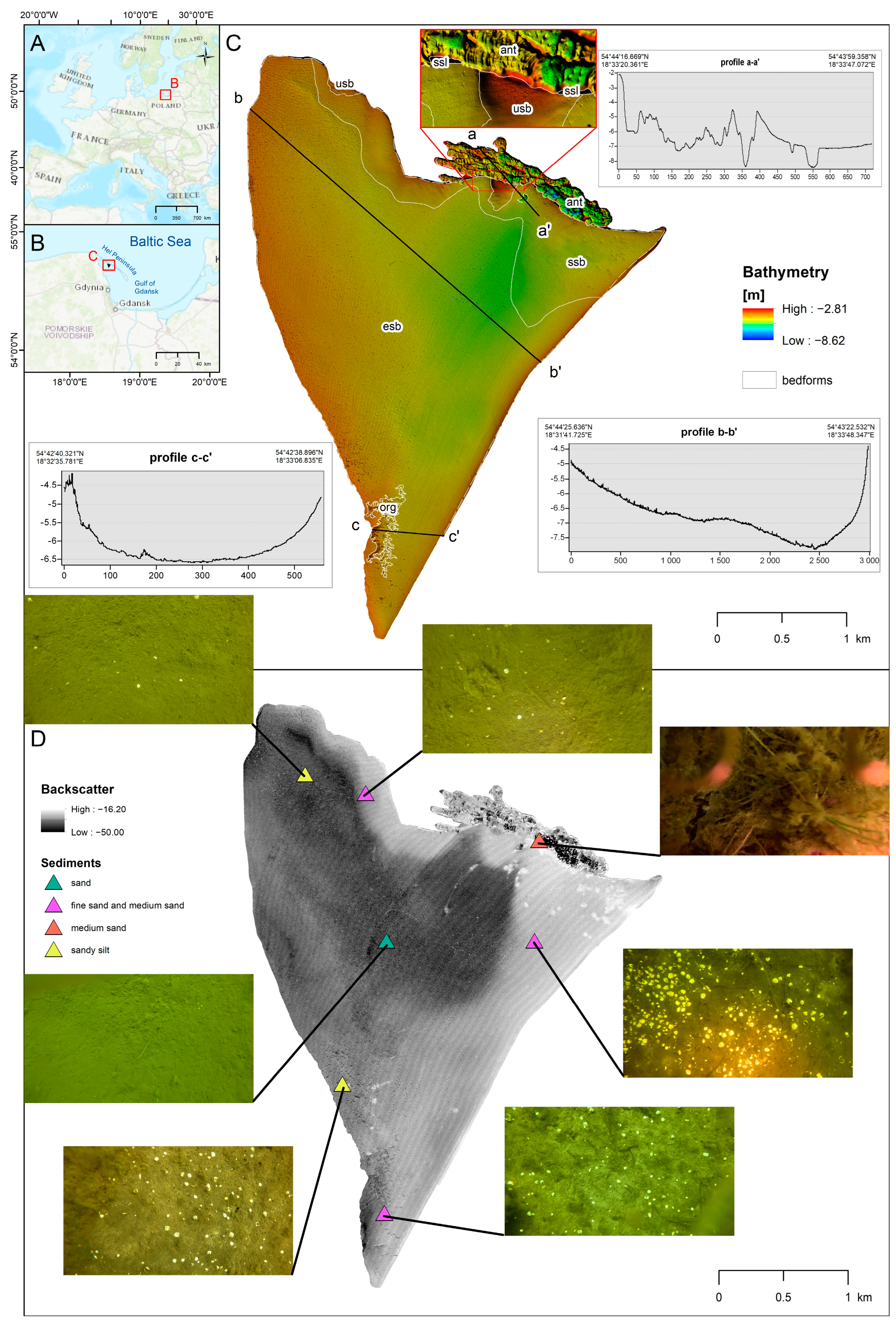
The Kuźnica Deep is situated in the northeastern part of the Puck Lagoon, a semi-enclosed geographical feature in the western Gulf of Gdańsk, separated from the open Baltic Sea by the Hel Peninsula to the northeast (Figure 1B).
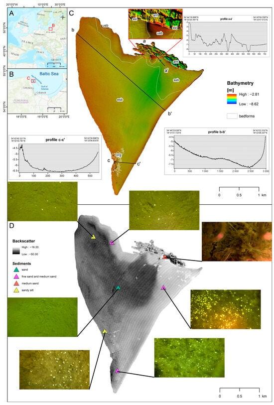
Figure 1.
Overview of the study site: (A) location of the study area within Europe; (B) location of the study area within northern Poland; (C) bathymetry of the Kuźnica Deep, showing three cross-profiles and the spatial arrangement of bedforms: ant—anthropogenic formations; org—accumulations of organics; usb—undulating seabed; ssb—slightly undulating seabed; esb—flat, even seabed; ssl—steep slopes; (D) backscatter of the Kuźnica Deep, indicating the locations of sediments and sites of grab samples and video recordings.
To the southeast, the deep is bordered by the Seagull Sandbar, which partially emerges during the year. To the west, it is separated by very shallow sandy shoals with mega ripple marks, reaching depths of approximately −1 m. The Kuźnica Deep is accessible for marine surveys from the southern part, where depths reach around −2.3 m. It spans approximately 7 km2, with depths of up to −8.62 m, making it one of the deepest areas of the Puck Lagoon.
Anthropogenic activities, such as dredging, have left visible remnants in the bathymetry, particularly in the northeastern part of the deep, where slopes incline up to approximately 26° (Figure 1C, profile a–a′). These areas, marked as ‘ant’ bedforms, contain numerous anthropogenic features, such as pipes and other artificial structures. While most of the area features a flat, uniform seabed (marked as ‘esb’; Figure 1C, profile b–b′), it transitions to a slightly undulating seabed (‘ssb’) near the anthropogenic scours, with small gentle sandy waves to clear sandy waves (‘usb’). Before reaching the anthropogenic scours, the seabed locally transforms into a steep slope (‘ssl’) with inclinations of up to 25°. In the southwestern part of the deep, near the survey entrance, there is a large area with accumulations of organic matter (mostly dead material, ‘org’), covering 0.07 km2 (7 ha, Figure 1C, profile c–c′). The origin of these accumulations was captured in a video recording of the surrounding area, with a sample located in the southern part of the area. A comprehensive investigation of all described bedforms, including the methodologies used for their determination, was provided by Janowski and Wróblewski [15] and is summarized in Table 1.

Table 1.
List of classes distinguished in this study with their descriptions and division into different categories.
Detailed knowledge of the Kuźnica Deep seafloor was obtained through high-resolution underwater remote sensing using an MBES. These measurements were conducted aboard the small IMOROS 3 survey motorboat, which was equipped with a Teledyne Reson T20-P MBES device (Teledyne Technologies, Thousand Oaks, CA, USA). The survey spanned three months, from March 22 to June 22, 2022, encompassing 21 days of data collection.
The measurement system included GPS receivers (Trimble SPS851 and Trimble BX982 (Trimble Inc., Sunnyvale, CA, USA)), an iXBlue Hydrins Inertial Navigation System (STR, Great Yarmouth, UK), a Reson SVP70 Sound Velocity Probe (Teledyne Technologies, Thousand Oaks, CA, USA), and a Reson SVP15 Sound Velocity Profiler (Stema Systems, Houten, The Netherlands). All measurements were performed with Real-Time Kinematic (RTK) corrections available throughout the survey area. Data collection was managed using QINSy 8.18 software, with the MBES configured to 999 beams, a frequency of 420 kHz, a pulse length of 30 μs, absorption of 70 dB/km, spreading of 35 dB, a swath angle of 130–140°, power of 220 dB, and a gain of 0 dB.
To ensure high-quality data, the MBES sensors were calibrated for time, pitch, roll, and yaw offsets and were regularly checked. The sound velocity was measured with the SVP15 at least every six hours, whenever environmental conditions changed, and before and after each measurement session. The survey ensured overlap between ship track lines and a consistent speed of 2–2.5 m/s. The MBES data were recorded in the PL-EVRF2007-NH vertical system and the PUWG1992 projected coordinate system, based on the ETRS89 ellipsoid.
The raw bathymetry data from the MBES were processed using Beamworx Autoclean 1.3 software (BeamworX B.V., Utrecht, The Netherlands). This process involved applying a Surface Spline filter to automatically eliminate outlier soundings. Additionally, the Shift Pings to Neighbors filter was used, which adjusts survey lines to align with neighboring lines using a best-fit algorithm, provided there is some overlap. Any remaining erroneous soundings were manually removed. As a result, bathymetry DEM (Digital Elevation Model) was developed in raster grid format.
For processing MBES backscatter data, Fledermaus Geocoder Toolbox (FMGT) (Quality Positioning Services BV (QPS), Zeist, The Netherlands) software was utilized. The cleaned MBES soundings and the bathymetric surface were imported into an FMGT project. An Angle Varying Gain (AVG) filter was applied to correct backscatter measurements for angular variations, using a 300-pings sliding window and the “flat” algorithm. All radiometric and geometric corrections were automatically applied with default settings. Finally, all bathymetry and backscatter datasets were exported to surface grids in GeoTiff format with a 0.2 m resolution.
The Bathymetry GeoTIFF was used as the primary feature for calculating secondary geomorphometric features (or terrain attributes), as listed and referenced in Table 2. All these features were generated using SAGA GIS software v.9.7.2 (open-source, manufactured by international developer community), specifically utilizing the “Morphometry” and “Lighting, Visibility” tool libraries. Additionally, MBES backscatter intensity GeoTIFF was employed for the determination of gray-level co-occurrence matrices (GLCMs) as well as gray-level difference vectors (GLDVs), also listed in Table 2. All texture features (or textural attributes) were calculated in all directions using Trimble eCognition software (https://geospatial.trimble.com/en/products/software/trimble-ecognition, Trimble Inc., Sunnyvale, CA, USA).

Table 2.
List of secondary geomorphometric and textural features extracted in this study.
The primary features of MBES measurements (bathymetry and backscatter) served as the main layers for multiresolution segmentation, which is the key algorithm within the OBIA framework [42]. This algorithm merges image pixels with similar spectral properties, guided by parameters such as scale, shape, and compactness [43]. The process starts with individual pixels and gradually groups these into larger segments until a certain level of heterogeneity is reached. This ensures that the resulting image objects are meaningful and visually coherent, much like how humans perceive images. By adjusting the parameters to fit specific datasets, the algorithm’s effectiveness is enhanced, ensuring optimal segmentation results. This approach helps to reduce the impact of environmental and physical factors on high-resolution images, which can affect pixel-level measurements. By creating image objects, OBIA provides detailed information, including texture and shape characteristics, making it particularly effective for high-resolution remote sensing images with diverse pixel information.
The first step of OBIA is segmentation, which was performed using a multiresolution segmentation algorithm with the following parameters: shape—0.1, compactness—0.5, scale—10, and image layer weights: BBS—2, DEM—1. These settings generated 211,723 image objects that were small enough to capture the spatial arrangement of ground truth control points. Additionally, since the DEM has much less spatial variability than BBS, increasing the layer weight of BBS to 2 allowed for the capture of specific variations in seabed properties. Finally, the image segments were subjected to machine learning supervised classification and then the output areas were merged.
In addition to underwater acoustic and geomorphometric datasets, the area was sampled using a small Van Veen grab and investigated with a GoPro camera mounted on a custom-designed sampler. Samples were strategically collected from seven carefully selected locations (Figure 1D). Sediment samples underwent sieve analysis, and for samples with more than 5% of material finer than 0.063 mm, a combined sieve and hydrometer test was performed. All these procedures were carried out in the accredited laboratories of the Offshore Geotechnics Department at the Maritime Institute of Gdynia Maritime University. These samples were used as a precondition for in situ validation and interpretation of the results.
The results of the manual bedform classification developed in a previous study [15] served as the basis for generating bathymetric control points tailored to the spatial extent of the Kuźnica Deep. The bedform classes were determined based on a combination of geomorphometric analysis and expert knowledge from previous studies. Each class was defined to capture distinct morphological and sedimentological characteristics observed in the study area. The rationale behind delineating these classes was to provide a comprehensive understanding of the seafloor’s physical structure. To prevent an over-density of points in small areas and ensure an even distribution across the study area, the number of control points was adjusted based on the percentage area of each class within the study area (Table 3). The control points were generated using the “Create Random Points” tool in ArcGIS software v.10.8.2 (Environmental Systems Research Institute (ESRI), Redlands, CA, USA). A total of 49,999 control points were extracted in the research area, serving as input for the Boruta feature selection algorithm, as well as for training and validating machine learning algorithms. The ratio between training and validation samples was set to 70/30, and they were separated randomly using the “Subset Features” tool in ArcGIS.

Table 3.
List of all control points by class with their corresponding area and their quantity.
To ensure that the machine learning algorithms achieved high performance, the Boruta feature selection algorithm was applied for all secondary features, using active variables based on control points [44]. In this modeling context, “features” refers to variables as defined by the Boruta algorithm, and not to the shapes of actual seafloor terrain features. Before applying the Boruta feature selection algorithm, cross-correlation was performed for all geomorphometric and textural features developed in the study. This step was crucial to identify and mitigate any multicollinearity among the features, ensuring that the subsequent feature selection process was both effective and reliable. The cutoff threshold for highly correlated features was set at 0.75 [45,46]. Only features with lower cross-correlation were subjected to the Boruta feature selection algorithm. This algorithm is designed to select all features that are important for a given classification task [44]. It works by iteratively comparing the importance of original features with that of random, shadow features. This method ensures that only the truly relevant features are retained, thereby improving the model’s accuracy and robustness. The Boruta algorithm has been widely used due to its strengths in handling high-dimensional data and its robustness against overfitting. However, it can be computationally intensive and may require significant processing time [47]. The Boruta algorithm was selected due to its effectiveness in ensuring high performance of machine learning algorithms by retaining only the most relevant features.
After receiving the feature selection results, Trimble eCognition software was utilized to test the following machine learning algorithms: Classification and Regression Trees (CARTs; [48]), Support Vector Machine (SVM; [49,50]), Random Forest (RF; [51]), Bayes [52] and k-Nearest Neighbor (KNN; [53]). These algorithms were applied to the image segmentation results to enable the automatic classification of underwater acoustic remote-sensing data. Their performance was then evaluated in the same software using error matrices and accuracy assessment metrics [54,55]. The processing parameters of each classifier (like max tree number, depth, kernel type, etc.) were tuned to achieve the highest possible accuracy.
3. Results
3.1. Feature Extraction and Cross-Correlation
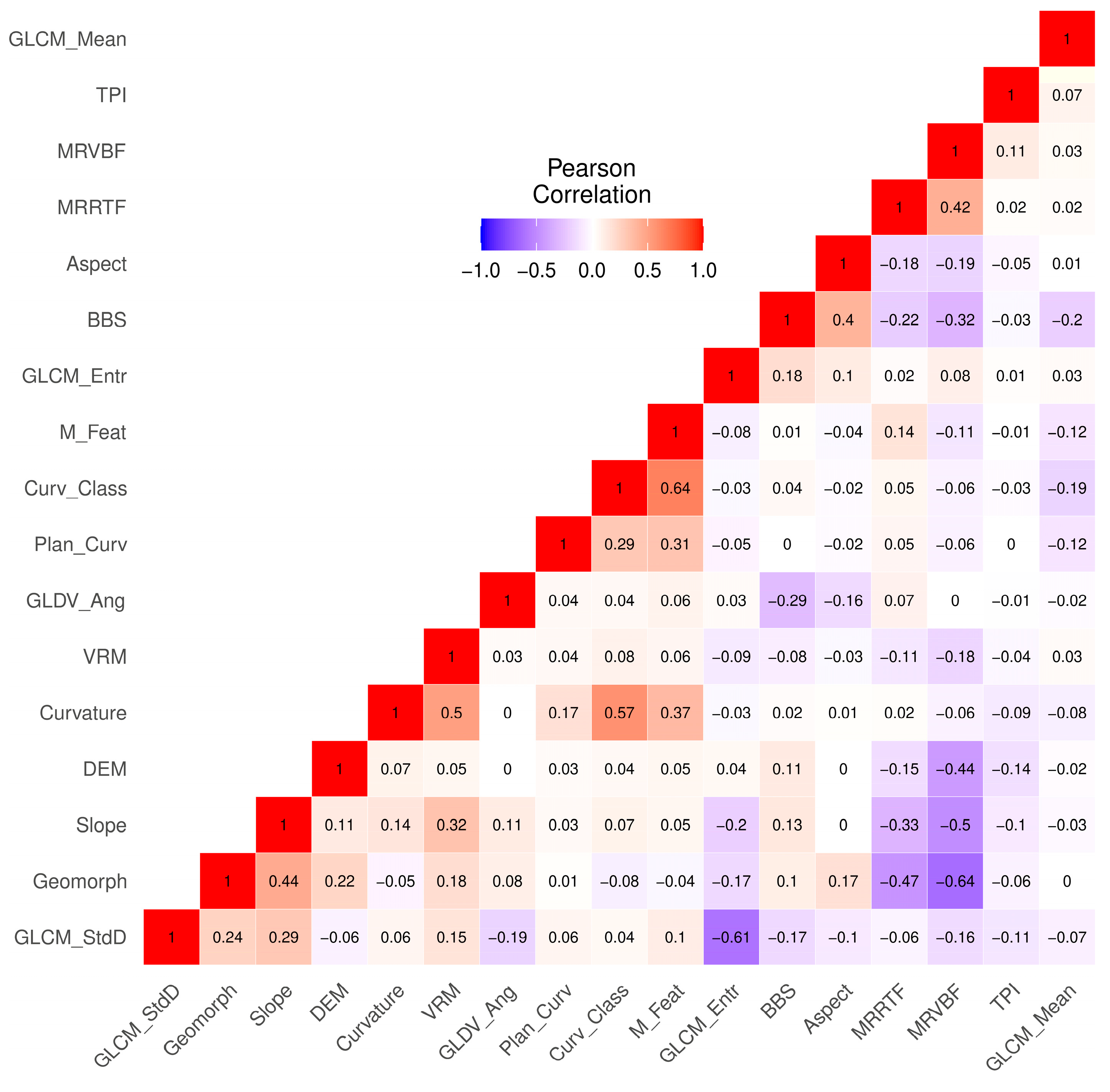
Cross-correlation identified features with correlations exceeding the threshold of 0.75 across the entire feature space, as listed in Table 4. As can be seen, the procedure helped remove 2 out of 13 geomorphometric features and 9 out of 12 textural features. Conversely, Figure 2 presents the cross-correlation diagram for the remaining subset of non-correlated features.

Table 4.
List of all highly correlated geomorphometric and textural features that were not utilized in the following modeling in this study.
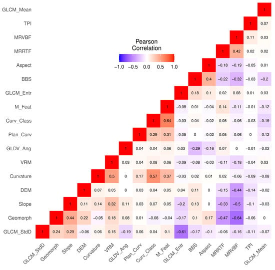
Figure 2.
Cross-correlation diagram showing non-correlated features and their statistics. Used abbreviations: GLCM_StdD—GLCM Standard Deviation; Geomorph—Geomorphons; GLDV_Ang—GLDV Angular 2nd Moment; Plan_Curv—Planar Curvature; Curv_Class—Curvature Classification; M_Feat—Morphometric Features; GLCM_Entr—GLCM Entropy; BBS—Backscatter mosaic; MRRTF—Multiresolution Index of the Ridge Top Flatness; MRVBF—Multiresolution Index of Valley Bottom Flatness; GLCM_Mean—GLCM Mean.
3.2. Feature Selection
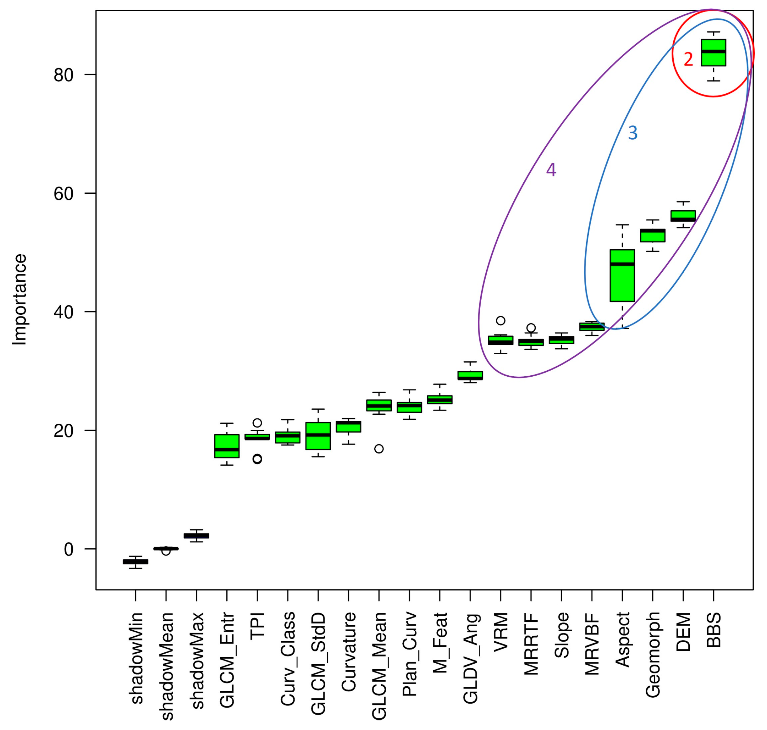
The results of the Boruta feature selection algorithm are shown in Figure 3. It can be seen that all the features are important, as they have higher importance than the best shadow feature and are considered significant. No features were marked as rejected or tentative. The features with the highest importance are the primary features (MBES backscatter mosaic and MBES bathymetry DEM) and some geomorphometric features, such as Geomorphons, Aspect, and the Multiresolution Index of Valley Bottom Flatness (MRVBF).
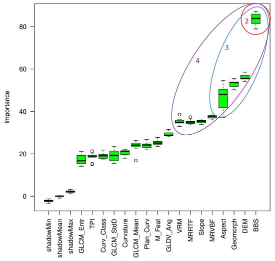
Figure 3.
Diagram of Boruta feature selection algorithm results displaying the results of each feature input. The ellipses circle the variables corresponding to clusters 2–4. Used abbreviations: GLCM_StdD—GLCM Standard Deviation; Geomorph—Geomorphons; GLDV_Ang—GLDV Angular 2nd Moment; Plan_Curv—Planar Curvature; Curv_Class—Curvature Classification; M_Feat—Morphometric Features; GLCM_Entr—GLCM Entropy; BBS—Backscatter mosaic; MRRTF—Multiresolution Index of the Ridge Top Flatness; MRVBF—Multiresolution Index of Valley Bottom Flatness; GLCM_Mean—GLCM Mean.
From the diagram in Figure 3, it is evident that the features form groups or clusters based on their importance. The first group may contain only the BBS feature, the second group includes DEM, Geomorphons, and Aspect, and the third cluster adds the Multiresolution Index of Valley Bottom Flatness, Slope, Multiresolution Index of the Ridge Top Flatness, and VRM. These results enabled the performance of machine learning supervised classification tasks with a better understanding of the feature space. Various models of input features were tested, including (1) all important features, (2) only BBS, (3) the first and second clusters, and (4) clusters 1–3 (Table 5).

Table 5.
List of all input feature space models tested in this study.
3.3. Supervised Classification Parameters Tuning
The comparison of machine learning classification results for the four models was initially conducted using the default settings of the classifiers, as listed in Table 6. Note that the naïve Bayes classifier, due to its simplicity, does not have any parameters to define and is, therefore, not included in Table 6.

Table 6.
List of all classifiers and their default settings.
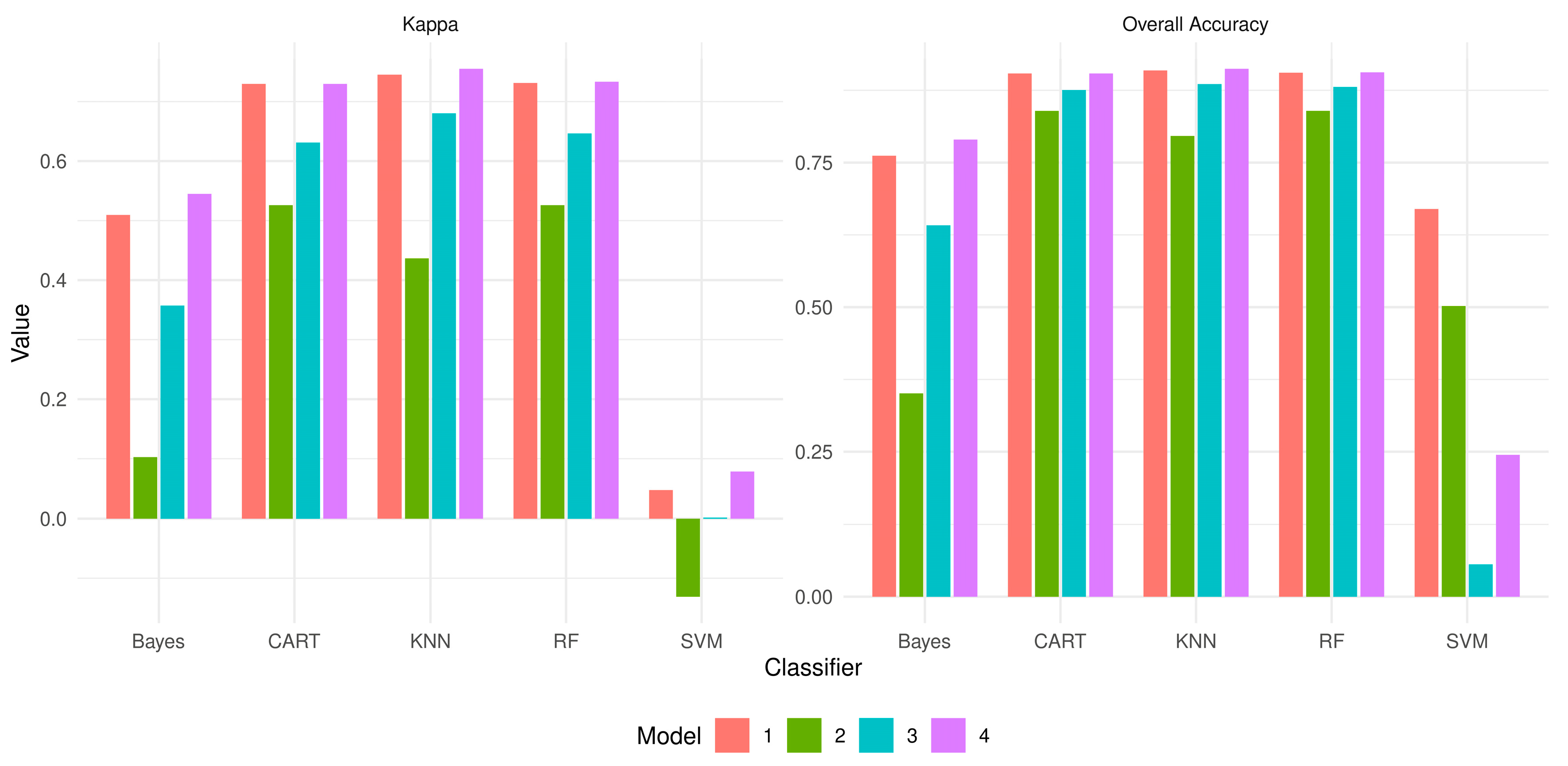
Accuracy assessment results, including the Overall Accuracy and the Kappa metrics, are shown in Figure 4. It was found that the CART, KNN, and RF classifiers consistently achieved the highest mean Overall Accuracy, all at around 0.88, and also exhibited high mean Kappa values, suggesting strong agreement. In contrast, the Bayes classifier showed moderate performance with a mean Overall Accuracy of approximately 0.64 and a moderate Kappa value. The SVM classifier, however, was found to perform poorly, with a mean Overall Accuracy of around 0.37 and a very low mean Kappa value close to zero, indicating poor agreement and high variability in performance. The CART, KNN, and RF classifiers were demonstrated to have robust and reliable performance across the models, making them the top choices. The Bayes classifier, while not as strong, still showed reasonable performance. However, the SVM classifier’s performance was notably weak, highlighting its inconsistency and lack of reliability in this context.
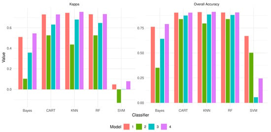
Figure 4.
Diagrams of Overall Accuracy and Kappa accuracy assessment statistics for various classifiers and models with the default classifier settings.
However, it should be noted that some parameters in default settings may not represent the full variability of the feature space, and this was the case for some of the features in this study. Therefore, we decided to introduce slightly changed settings (Table 7), mainly by introducing feature space normalization in the SVM and KNN classifiers and by changing the depth and min sample count parameters for the CART and RF classifiers.

Table 7.
List of all classifiers and their slightly modified settings.
The accuracy assessment results for the model runs with the customized settings, including Overall Accuracy and Kappa metrics, are presented in Figure 5. In Model 1, it was observed that KNN achieved the highest performance with an overall accuracy of 0.91 and a Kappa of 0.75, while SVM performed the worst with an overall accuracy of 0.53 and a Kappa of 0.02. In Model 2, RF was identified as the best classifier with an overall accuracy of 0.84 and a Kappa of 0.53, whereas Bayes was noted to have the lowest performance with an overall accuracy of 0.35 and a Kappa of 0.10. For Model 3, KNN again emerged as the top performer with an overall accuracy of 0.91 and a Kappa of 0.74, while Bayes had the poorest performance with an overall accuracy of 0.64 and a Kappa of 0.36. In Model 4, KNN was found to be the best classifier with an overall accuracy of 0.94 and a Kappa of 0.84, and SVM was identified as the worst with an overall accuracy of 0.84 and a Kappa of 0.53.
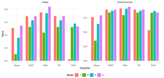
Figure 5.
Diagrams of Overall accuracy and Kappa accuracy assessment statistics for various classifiers and models with slightly modified classifier settings.
Overall, KNN was consistently noted to perform well across all models, often achieving the highest accuracy and Kappa values. In contrast, Bayes and SVM were observed to perform poorly in most models, with Bayes being the worst in Models 2 and 3, and SVM in Models 1 and 4.
Finally, the last approach involved testing further modified settings of supervised classifiers. In this attempt, the parameters for depth and minimum sample count were increased, and the maximum categories parameter for CART and RF was adjusted to match the known number of classes of ground-truth control points. Additionally, the kernel type for SVM was changed from linear to rbf (radial basis function), and the k factor in KNN was increased to 2 (Table 8).

Table 8.
List of all classifiers and their further modified settings.
Qualitative results for the main parameters of accuracy assessment are shown in Figure 6. It was found that the SVM classifier achieved the highest mean Overall Accuracy at 0.90, followed closely by the CART and RF classifiers, both with a mean Overall Accuracy of approximately 0.89. KNN also performed well with a mean Overall Accuracy of around 0.86. The Bayes classifier showed moderate performance with a mean Overall Accuracy of approximately 0.64. In terms of Kappa, the SVM classifier again led with the highest mean value of 0.71, indicating strong agreement. CART and RF classifiers also showed high mean Kappa values of around 0.67, while KNN had a mean Kappa value of approximately 0.65. The Bayes classifier had a moderate mean Kappa value of around 0.38.
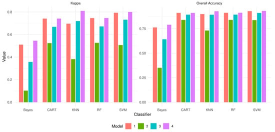
Figure 6.
Diagrams of Overall accuracy and Kappa accuracy assessment statistics for various classifiers and models with further modified settings.
The standard deviation for Overall Accuracy and Kappa was relatively low for the CART, RF, and SVM classifiers, indicating consistent performance. KNN showed a slightly higher standard deviation, suggesting some variability in its performance. The Bayes classifier had the highest standard deviation, indicating the most variability in performance. The SVM classifier demonstrated the best overall performance, both in terms of mean Overall Accuracy and Kappa, with consistent results. CART and RF classifiers also performed very well, showing high accuracy and agreement with low variability. KNN performed well but with slightly more variability. The Bayes classifier showed moderate performance with the highest variability among the classifiers.
3.4. Analysis of Accuracy Assessment
The results were analyzed quantitatively to determine the best model and classifier based on Overall Accuracy and Kappa for each approach. In Approach 1 (default settings of classifiers), the KNN classifier in Model 4 was identified as the best, with an Overall Accuracy of 0.91 and a Kappa of 0.76. For Approach 2 (slightly modified settings of classifiers), the KNN classifier in Model 4 was found to be superior, achieving an Overall Accuracy of 0.94 and a Kappa of 0.84. In Approach 3 (further modified settings of classifiers), the SVM classifier in Model 4 was deemed the best, with an Overall Accuracy of 0.93 and a Kappa of 0.80.
In comparison, the best performance of the RF classifier was observed in Approach 3, Model 4, with an Overall Accuracy of 0.91 and a Kappa of 0.75. The best performance of the CART classifier was observed in Approach 3, Model 4, with an Overall Accuracy of 0.91 and a Kappa of 0.74. Moreover, the best performance of the Bayes classifier was consistently observed in Model 4 across all three approaches (there are no parameters to define in the Bayes classifier), with an Overall Accuracy of 0.79 and a Kappa of 0.54. However, these results were lower compared to the best classifiers in each approach, particularly the KNN classifier in Approach 2, Model 4, which had the highest Overall Accuracy and Kappa among all classifiers and approaches.
Based on the analysis, Model 4 demonstrated the highest performance across all scenarios. Consequently, the error matrices and accuracy assessment results from Model 4 for the classification methods were further examined to provide insights into misclassifications, overclassifications, and other interpretations of accuracy results.
For Approach 1 using KNN, high misclassifications were observed in the ‘ssb’ and ‘usb’ classes, while the ‘org’ class exhibited low producer accuracy, indicating many samples were misclassified into other classes. Overclassification was noted in the ‘esb’ class, which had a high user accuracy but still showed some overclassification into ‘ssb’ and ‘org’ (Figure 7a). In Approach 2 using KNN, misclassifications were significantly reduced, especially in the ‘org’ class, which showed improved producer accuracy. The ‘usb’ class also performed better with higher producer accuracy. Overclassification in the ‘esb’ class was minimal, with a high user accuracy (Figure 7b). For Approach 3 using SVM, severe misclassification was noted in the ‘org’ class, which had very low producer accuracy. The ‘usb’ class also showed poor performance with low producer accuracy. Overclassification was present in the ‘esb’ class, which had a high user accuracy but still showed some overclassification into ‘ssb’ and ‘org’ (Figure 7c). In Approach 3 using RF, the ‘org’ class had low producer accuracy, indicating many samples were misclassified. The ‘usb’ class showed no correct classifications, indicating a major issue. Overclassification was seen in the ‘esb’ class, which had a high user accuracy but still showed some overclassification into ‘ssb’ and ‘org’ (Figure 7d). For Approach 3 using CART, severe misclassification was noted in the ‘org’ class, which had very low producer accuracy. The ‘usb’ class showed minimal correct classifications. Overclassification was present in the ‘esb’ class, which had a high user accuracy but still showed some overclassification into ‘ssb’ and ‘org’ (Figure 7e). In the Bayes approaches (1–3), the ‘org’ class had moderate producer accuracy but low user accuracy, indicating many samples were misclassified. The ‘usb’ class showed poor performance with low user accuracy. Overclassification was seen in the ‘esb’ class, which had a high user accuracy but still showed some overclassification into ‘ssb’ and ‘org’(Figure 7f).
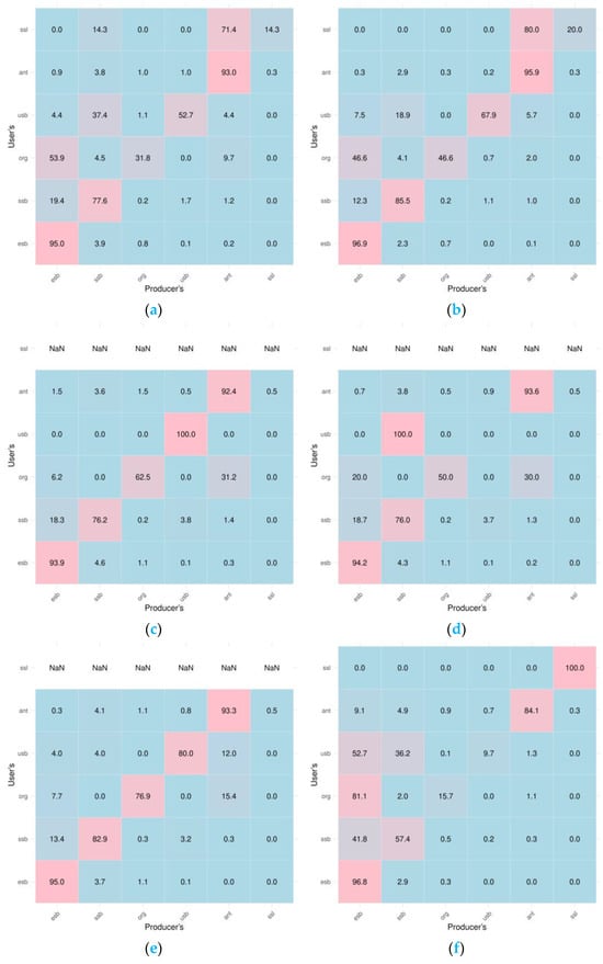
Figure 7.
Error matrices from Model 4, normalized for percentage values, highlighting the top-performing results of various classifiers across the three approaches: (a) approach 1, KNN; (b) approach 2, KNN; (c) approach 3, CART; (d) approach 3, RF; (e) approach 3, SVM; (f) approaches 1–3, Bayes. NaN (Not a Number)—there were no observations of validation samples for specific classes.
In summary, the KNN classifier showed good overall performance, especially in Approach 2 with high accuracy and Kappa values. SVM performed well overall but struggled with certain classes like ‘org’ and ‘usb’. RF generally showed good performance but had issues with specific classes like ‘usb’. CART had a similar performance to RF, with good overall accuracy but struggled with certain classes. Bayes methods had lower overall accuracy and Kappa, indicating more misclassifications and overclassifications compared to other methods.
3.5. Seabed Bedform Maps
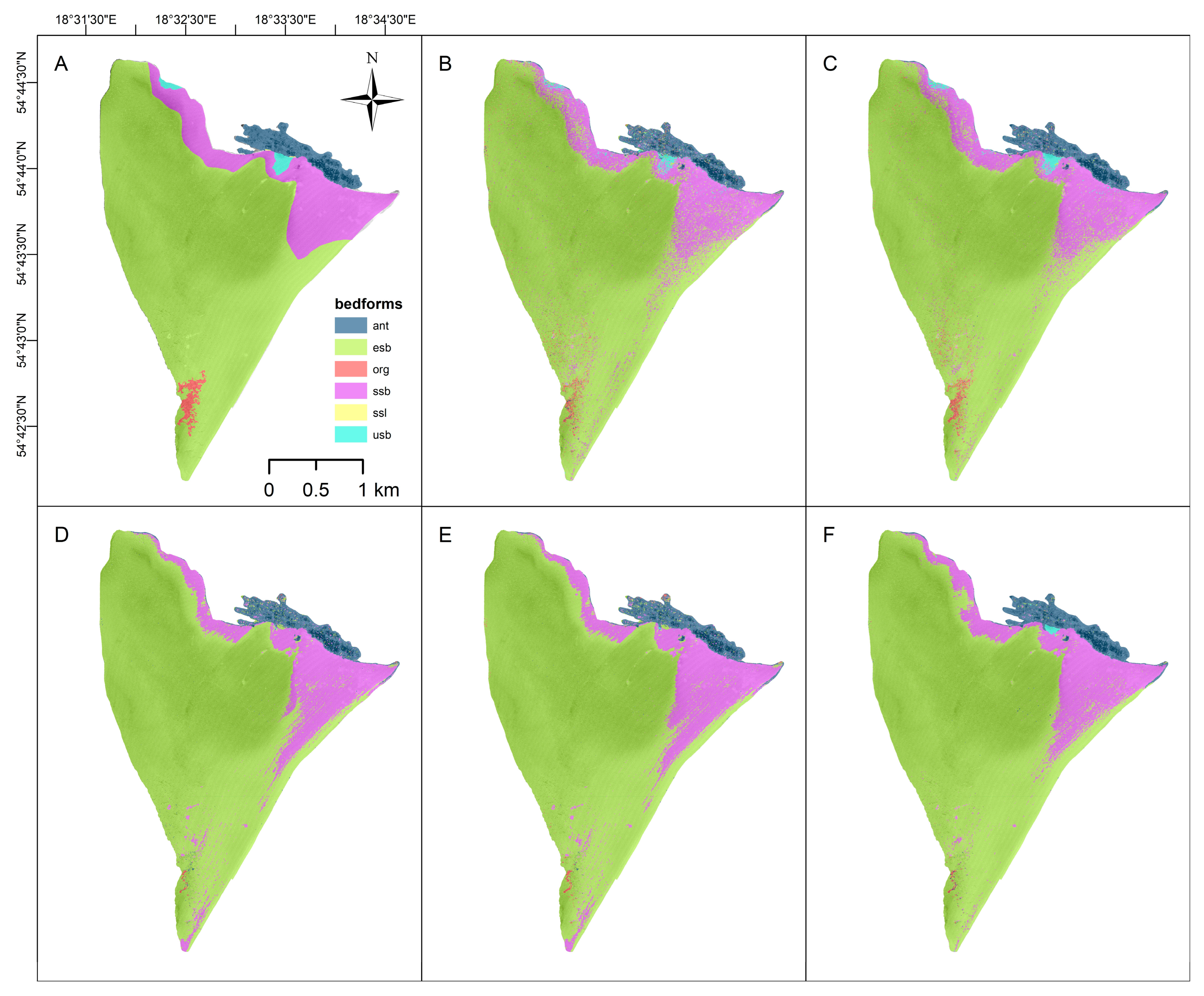
These analyses allowed the preparation of seabed bedform maps of the Kuźnica Deep (Figure 8). Because the result based on the Bayesian classifier was much lower performance, it was not presented in this figure.

Figure 8.
Seabed composition maps of the Kuźnica Deep layered over MBES backscatter primary feature: (A) result of manual classification; (B) approach 1, KNN; (C) approach 2, KNN; (D) approach 3, CART; (E) approach 3, RF; (F) approach 3, SVM.
4. Discussion
4.1. Implications of the Results
The feature selection results from this study have several important implications for geomorphometric and textural analysis, as well as for the broader field of machine learning in geospatial research.
By applying the Boruta feature selection algorithm, the study ensured that only the most relevant features were retained. This process helps in reducing the dimensionality of the dataset, which can significantly enhance the performance of machine learning models. Models trained on a reduced set of relevant features are generally more accurate and robust, as they are less likely to overfit and can generalize better to new data. The clustering of features based on their importance, as identified by the Boruta algorithm, provides valuable insights into the relationships between different geomorphometric and textural features. This improved interpretability can help to understand the underlying processes and patterns in the data, leading to more informed decision-making and hypothesis generation.
The Boruta feature selection algorithm identified several key geomorphometric features from MBES bathymetry that are critical for seafloor bedform mapping. Features like Geomorphons, Aspect, and the Multiresolution Index of Valley Bottom Flatness were found to be highly important. These features help in distinguishing different seafloor types and understanding the spatial distribution of sediments, thereby aiding in accurate seafloor composition mapping [45,56].
Conversely, the importance of textural features was much less significant compared to the geomorphometric alternatives. Given the highest value of MBES backscatter, which significantly outperformed all other secondary features, it is quite surprising that none of the textural features (generated from BBS) ranked higher [57,58]. Therefore, in the case of Kuźnica Deep, textural features did not have as high discriminatory power as backscatter.
It should be kept in mind that GLCMs/GLDVs are calculated for specific directions. While this study calculated all textural features in all directions, it is also possible to generate GLCMs in specific directions (0°, 45°, 90°, 135°), which may impact the feature space. However, considering that the calculation of any Haralick texture feature is very processor-intensive due to the GLCM calculation, performance may suffer. In this study, we calculated only GLCMs/GLDVs in all directions. Future studies may consider other variants of GLCMs/GLDVs [41]. It is important to note that backscatter measurements can be significantly influenced by the orientation of the multibeam survey lines relative to the seafloor, the data collection settings, and the sonar frequency [59]. Consequently, the ability of a backscatter dataset to accurately characterize substrates may be impacted by the specific methods used during data collection.
Overall, the feature selection results underscore the importance of careful and systematic feature selection in geospatial analysis. By enhancing model performance, improving computational efficiency, and providing better interpretability, these results contribute to the advancement of machine learning applications in geomorphometry and beyond. The analysis indicated that including all features (Model 1) does not necessarily lead to the best performance. In fact, Model 4, which included only the eight most important features, often showed better performance than Model 1. This suggests that further selection (after feature selection) can play a crucial role in improving classifier performance. By focusing on the most important features, it is possible to achieve high accuracy and Kappa values while potentially reducing computational complexity and overfitting [60]. Therefore, it is not always necessary to consider all important features for classification, and a well-thought-out feature selection process can lead to more efficient and effective models [32,61,62].
From analyses of supervised classification qualitative results, it can be concluded that RF and KNN are reliable choices for classification tasks, as they consistently deliver high accuracy and Kappa values across different settings [63]. CART also proves to be a strong performer, though slightly less robust than RF and KNN. Bayes, while not the top performer, provides moderate results that could be useful in certain contexts. Conversely, SVM demonstrates the need for careful parameter tuning to achieve optimal results, as its performance varied significantly across the different approaches [64]. This analysis highlights the importance of tuning classifier settings to achieve the best performance and suggests that some classifiers are more sensitive to these changes (SVM) than others (KNN/CART/RF).
The study demonstrates how recent advancements in remote sensing technologies, such as OBIA and machine learning algorithms like KNN and RF, improve geospatial data analysis. These technologies enable the extraction of detailed and relevant features from large datasets, enhancing the precision and reliability of underwater landscape analysis. The integration of these advanced methods allows for more sophisticated and accurate mapping of the Kuźnica Deep. The implications of this study highlight the significance of feature selection and advanced machine learning techniques in improving the accuracy and efficiency of geospatial data analysis, particularly for nearshore underwater landscapes like the Kuźnica Deep [65,66,67].
4.2. Comparison with Hierarchical Classification Approach
Benthic habitat mapping often employs hierarchical classification approaches to systematically categorize seabed features from the largest to the smallest scales [28]. This method involves multiple levels of classification, starting with broad categories such as major geomorphological features (e.g., continental shelves, slopes, and basins) and progressively refining down to more specific features like sediment types, biological communities, and microhabitats. Each level of the hierarchy provides a more detailed understanding of the seabed, allowing for precise mapping and analysis [68]. The integrated classification approach adopted in this study, which combines both geomorphological and other categories, offers a comprehensive understanding of seabed features. By classifying all features together in one round, this approach avoids the potential pitfalls of hierarchical classification, such as the misclassification of features due to scale-dependent criteria. This comprehensive method ensures that the classification is robust, reproducible, and reflective of the actual seabed conditions, making it a valuable tool for benthic habitat mapping.
4.3. Limitations of the Research
The determination of the ‘org’ class, representing accumulations of organic matter, presents several limitations and challenges. Firstly, organic accumulations exhibit a high degree of complexity and variability in their acoustic signatures due to differences in composition, density, and distribution. This variability makes it difficult for automated classifiers to consistently distinguish these features from other seabed types. Additionally, the limited ground-truth data available for training the classifiers may have contributed to lower accuracy in identifying the ‘org’ class. Although a larger dataset of control points was used, the inherent variability in organic accumulations requires more extensive ground truth data to improve classification accuracy. Furthermore, the sensitivity of machine learning classifiers to parameter settings can impact their performance, as evidenced by the varying results across different classifiers and parameter adjustments. Lastly, the features used for classification, such as backscatter intensity and geomorphometric attributes, may not fully capture the unique characteristics of organic accumulations. Future research should explore additional features or alternative data sources to enhance the classification of this complex seabed feature. These challenges highlight the need for ongoing refinement of classification methods to achieve more accurate and reliable results.
4.4. Reference to Main Research Questions
This research provided answers to the questions raised in the Introduction. The Kuźnica Deep features a flat, uniform seabed in most areas, transitioning to a slightly undulating seabed near anthropogenic scours. The northeastern part has slopes inclining up to 30°, with numerous anthropogenic features like pipes and artificial structures. The southwestern part contains a large area with accumulations of organic matter, covering 0.07 km2 (7 ha).
The MBES backscatter mosaic was one of the primary features with high importance for seabed characterization. It captured specific variations in seabed properties, which were crucial for the segmentation and classification processes in OBIA and machine learning tasks. The MBES backscatter was identified as having the highest value among the features, significantly outperforming other secondary features. This indicated that backscatter intensity measurements were crucial for distinguishing different seafloor types, thereby aiding in accurate seafloor composition mapping [69,70].
The most important geomorphometric features included Geomorphons, Aspect, MRVBF, Slope, MRRTF, and VRM. These features, along with MBES backscatter mosaic and MBES bathymetry DEM, formed clusters based on their importance and contributed significantly to the classification tasks.
Recent advancements in remote sensing technologies, such as OBIA and machine learning algorithms, improve geospatial data analysis by enabling the extraction of detailed and relevant features from large datasets. These technologies enhance the precision and reliability of underwater landscape analysis, allowing for more sophisticated and accurate mapping. OBIA and machine learning improved geospatial data analysis by enabling detailed segmentation and classification of seabed features. The use of multiresolution segmentation algorithms and supervised classification tasks allowed a better understanding and mapping of the underwater landscape. Machine learning models, such as KNN, RF, and SVM, have shown robust performance in classifying seabed features. The use of different approaches and modified settings improved the accuracy and reliability of the classification results.
The improved classification methods and feature selection processes can be applied to similar environments, enhancing the accuracy and reliability of seabed mapping and analysis. The findings underscore the importance of careful and systematic feature selection in geospatial analysis, which enhances model performance, improves computational efficiency, and provides better interpretability. This contributes to the advancement of machine learning applications in geomorphometry.
5. Conclusions
This study provides a comprehensive analysis of modeling methods applied to the characterization of the underwater landscape of the Kuźnica Deep, utilizing advanced remote sensing technologies. The key characteristics of bathymetry and backscatter intensity measurements from MBES were identified, significantly enhancing seabed mapping accuracy. Crucial geomorphometric features derived from MBES bathymetry were highlighted, offering valuable insights for classifying seafloor bedforms.
The integration of OBIA and machine learning techniques has markedly improved the sophistication of seabed geospatial data analysis, enabling more precise and detailed underwater landscape assessments. These advancements support a wide range of hydrographic, ecological, and geological research, offering a robust framework for future studies in the Kuźnica Deep and similar environments. The findings underscore the importance of leveraging cutting-edge technologies to advance our understanding of complex underwater ecosystems.
Funding
This research was funded in whole or in part by the National Science Centre, Poland [Grant number: 2021/40/C/ST10/00240]. The APC was funded by Gdynia Maritime University [project number: IM/2025/PZ/03].
Data Availability Statement
All remote sensing datasets utilized in this paper can be assessed through the Marine Geoscience Data System [14].
Acknowledgments
The author would like to acknowledge the competent assistance of the crews of the research vessels IMOROS 2 and IMOROS 3 during the surveys. Additionally, the author extends gratitude to the Offshore Geotechnics Department of the Maritime Institute at Gdynia Maritime University for their laboratory services in sediment analysis.
Conflicts of Interest
The author declares no conflicts of interest. The funders had no role in the design of the study; in the collection, analyses, or interpretation of data; in the writing of the manuscript; or in the decision to publish the results.
References
- Jones, D.O.B.; Gates, A.R.; Huvenne, V.A.I.; Phillips, A.B.; Bett, B.J. Autonomous marine environmental monitoring: Application in decommissioned oil fields. Sci. Total Env. 2019, 668, 835–853. [Google Scholar] [CrossRef] [PubMed]
- Wölfl, A.-C.; Snaith, H.; Amirebrahimi, S.; Devey, C.W.; Dorschel, B.; Ferrini, V.; Huvenne, V.A.I.; Jakobsson, M.; Jencks, J.; Johnston, G.; et al. Seafloor Mapping—The Challenge of a Truly Global Ocean Bathymetry. Front. Mar. Sci. 2019, 6, 283. [Google Scholar] [CrossRef]
- Mayer, L.; Jakobsson, M.; Allen, G.; Dorschel, B.; Falconer, R.; Ferrini, V.; Lamarche, G.; Snaith, H.; Weatherall, P. The Nippon Foundation—GEBCO Seabed 2030 Project: The Quest to See the World’s Oceans Completely Mapped by 2030. Geosciences 2018, 8, 63. [Google Scholar] [CrossRef]
- Zwolak, K.; Wigley, R.; Bohan, A.; Zarayskaya, Y.; Bazhenova, E.; Dorshow, W.; Sumiyoshi, M.; Sattiabaruth, S.; Roperez, J.; Proctor, A.; et al. The Autonomous Underwater Vehicle Integrated with the Unmanned Surface Vessel Mapping the Southern Ionian Sea. The Winning Technology Solution of the Shell Ocean Discovery XPRIZE. Remote Sens. 2020, 12, 1344. [Google Scholar] [CrossRef]
- UNESCO-IOC. Ocean decade Bathymetry Data Sharing Guideline. Ocean Decade Ser. 2024, 58, 1–14. [Google Scholar]
- Węsławski, J.; Rzemykowska, H. Zatoka Pucka. In Atlas of Polish Marine Area Bottom Habitats; Gic-Grusza, G., Kryla-Straszewska, L., Urbanski, J., Warzocha, J., Weslawski, J.M., Eds.; Broker-Innowacji: Gdynia, Poland, 2009; pp. 97–128. [Google Scholar]
- Węsławski, J.M.; Kryla-Straszewska, L.; Piwowarczyk, J.; Urbański, J.; Warzocha, J.; Kotwicki, L.; Włodarska-Kowalczuk, M.; Wiktor, J. Habitat modelling limitations—Puck Bay, Baltic Sea—A case study. Oceanologia 2013, 55, 167–183. [Google Scholar] [CrossRef]
- Nowacki, J. Cyrkulacja i wymiana wód. In Zatoka Pucka; Korzeniewski, K., Ed.; Instytut Oceanografii UG: Gdańsk, Poland, 1993; pp. 181–206. [Google Scholar]
- Szmytkiewicz, A.; Szymczak, E. Sediment deposition in the Puck Lagoon (Southern Baltic Sea, Poland). Baltica 2014, 27, 105–118. [Google Scholar] [CrossRef]
- Kruk-Dowgiałło, L.; Opioła, R. Program Rekultywacji Eyrobisk w Zatoce Puckiej: Przyrodnicze Podstawy i Uwarunkowania. 2009. Available online: https://repozytorium.bg.ug.edu.pl/info/book/UOG133eab2cabd440e2b21a0429baaa2a1f/ (accessed on 12 December 2024).
- Tegowski, J.; Gorska, N.; Klusek, Z. Statistical analysis of acoustic echoes from underwater meadows in the eutrophic Puck Bay (southern Baltic Sea). Aquat. Living Resour. 2003, 16, 215–221. [Google Scholar] [CrossRef]
- Jankowska, E.; Jankowska, K.; Włodarska-Kowalczuk, M. Seagrass vegetation and meiofauna enhance the bacterial abundance in the Baltic Sea sediments (Puck Bay). Environ. Sci. Pollut. Res. 2015, 22, 14372–14378. [Google Scholar] [CrossRef] [PubMed]
- Sokołowski, A.; Jankowska, E.; Balazy, P.; Jędruch, A. Distribution and extent of benthic habitats in Puck Bay (Gulf of Gdańsk, southern Baltic Sea). Oceanologia 2021, 63, 301–320. [Google Scholar] [CrossRef]
- Janowski, Ł.; Skarlatos, D.; Agrafiotis, P.; Tysiąc, P.; Pydyn, A.; Popek, M.; Kotarba-Morley, A.M.; Mandlburger, G.; Gajewski, Ł.; Kołakowski, M.; et al. High resolution optical and acoustic remote sensing datasets of the Puck Lagoon. Sci. Data 2024, 11, 360. [Google Scholar] [CrossRef]
- Janowski, Ł.; Wróblewski, R. Application and Evaluation of the AI-Powered Segment Anything Model (SAM) in Seafloor Mapping: A Case Study from Puck Lagoon, Poland. Remote Sens. 2024, 16, 2638. [Google Scholar] [CrossRef]
- Blaschke, T.; Hay, G.J.; Kelly, M.; Lang, S.; Hofmann, P.; Addink, E.; Queiroz Feitosa, R.; van der Meer, F.; van der Werff, H.; van Coillie, F.; et al. Geographic Object-Based Image Analysis—Towards a new paradigm. ISPRS J. Photogramm. Remote Sens. 2014, 87, 180–191. [Google Scholar] [CrossRef] [PubMed]
- Ierodiaconou, D.; Monk, J.; Rattray, A.; Laurenson, L.; Versace, V.L. Comparison of automated classification techniques for predicting benthic biological communities using hydroacoustics and video observations. Cont. Shelf Res. 2011, 31, S28–S38. [Google Scholar] [CrossRef]
- Legrand, H.; Lenfant, P.; Sotheran, I.; Foster-Smith, R.; Galzin, R.; Maréchal, J. Mapping marine benthic habitats in Martinique (French West Indies). Caribb. J. Sci. 2010, 46, 267–282. [Google Scholar] [CrossRef]
- Lucieer, V.; Lucieer, A. Fuzzy clustering for seafloor classification. Mar. Geol. 2009, 264, 230–241. [Google Scholar] [CrossRef]
- Ierodiaconou, D.; Schimel, A.C.G.; Kennedy, D.; Monk, J.; Gaylard, G.; Young, M.; Diesing, M.; Rattray, A. Combining pixel and object based image analysis of ultra-high resolution multibeam bathymetry and backscatter for habitat mapping in shallow marine waters. Mar. Geophys. Res. 2018, 39, 271–288. [Google Scholar] [CrossRef]
- Stephens, D.; Diesing, M. A comparison of supervised classification methods for the prediction of substrate type using multibeam acoustic and legacy grain-size data. PLoS ONE 2014, 9, e93950. [Google Scholar] [CrossRef]
- Kirillov, A.; Mintun, E.; Ravi, N.; Mao, H.Z.; Rolland, C.; Gustafson, L.; Xiao, T.T.; Whitehead, S.; Berg, A.C.; Lo, W.Y.; et al. Segment Anything. In Proceedings of the IEEE/CVF International Conference on Computer Vision (ICCV), Paris, France, 2–6 October 2023; pp. 3992–4003. [Google Scholar]
- Breyer, G.; Bartholomä, A.; Pesch, R. The Suitability of Machine-Learning Algorithms for the Automatic Acoustic Seafloor Classification of Hard Substrate Habitats in the German Bight. Remote Sens. 2023, 15, 4113. [Google Scholar] [CrossRef]
- Pratomo, D.G. Deep neural network based seafloor sediment mapping using bathymetric features of MBES multifrequency. Ocean Syst. Eng. 2024, 14, 101–114. [Google Scholar]
- Misiuk, B.; Brown, C.J. Benthic habitat mapping: A review of three decades of mapping biological patterns on the seafloor. Estuar. Coast. Shelf Sci. 2024, 296, 108599. [Google Scholar] [CrossRef]
- Brown, C.; Beaudoin, J.; Brissette, M.; Gazzola, V. Multispectral Multibeam Echo Sounder Backscatter as a Tool for Improved Seafloor Characterization. Geosciences 2019, 9, 126. [Google Scholar] [CrossRef]
- Ilich, A.R.; Misiuk, B.; Lecours, V.; Murawski, S.A. MultiscaleDTM: An open-source R package for multiscale geomorphometric analysis. Trans. GIS 2023, 27, 1164–1204. [Google Scholar] [CrossRef]
- Porskamp, P.; Rattray, A.; Young, M.; Ierodiaconou, D. Multiscale and Hierarchical Classification for Benthic Habitat Mapping. Geosciences 2018, 8, 119. [Google Scholar] [CrossRef]
- Blondel, P.; Prampolini, M.; Foglini, F. Acoustic Textures and Multibeam Mapping of Shallow Marine Habitatas—Examples from Eastern Malta; Institute of Acoustics: Milton, UK, 2015. [Google Scholar]
- Lecours, V.; Dolan, M.F.J.; Micallef, A.; Lucieer, V.L. A review of marine geomorphometry, the quantitative study of the seafloor. Hydrol. Earth Syst. Sci. 2016, 20, 3207–3244. [Google Scholar] [CrossRef]
- Lucieer, V.; Lecours, V.; Dolan, M. Charting the Course for Future Developments in Marine Geomorphometry: An Introduction to the Special Issue. Geosciences 2018, 8, 477. [Google Scholar] [CrossRef]
- Diesing, M.; Mitchell, P.; Stephens, D. Image-based seabed classification: What can we learn from terrestrial remote sensing? ICES J. Mar. Sci. J. Du Cons. 2016, 73, 2425–2441. [Google Scholar] [CrossRef]
- Zevenbergen, L.W.; Thorne, C.R. Quantitative analysis of land surface topography. Earth Surf. Process. Landf. 1987, 12, 47–56. [Google Scholar] [CrossRef]
- MacMillan, R.A.; Shary, P.A. Chapter 9 Landforms and Landform Elements in Geomorphometry. In Geomorphometry—Concepts, Software, Applications; Elsevier: Amsterdam, The Netherlands, 2009; pp. 227–254. [Google Scholar] [CrossRef]
- Schmidt, J.; Hewitt, A. Fuzzy land element classification from DTMs based on geometry and terrain position. Geoderma 2004, 121, 243–256. [Google Scholar] [CrossRef]
- Wood, J. The Geomorphological Characterisation of Digital Elevation Models; University of Leicester: Leicester, UK, 1996. [Google Scholar]
- Gallant, J.C.; Dowling, T.I. A multiresolution index of valley bottom flatness for mapping depositional areas. Water Resour. Res. 2003, 39, 1347. [Google Scholar] [CrossRef]
- Weiss, A.D. Topographic positions and landforms analysis. In Proceedings of the ESRI User Conference, San Diego, CA, USA, 14–18 July 2025. [Google Scholar]
- Sappington, J.M.; Longshore, K.M.; Thompson, D.B. Quantifying Landscape Ruggedness for Animal Habitat Analysis: A Case Study Using Bighorn Sheep in the Mojave Desert. J. Wildl. Manag. 2007, 71, 1419–1426. [Google Scholar] [CrossRef]
- Jasiewicz, J.; Stepinski, T.F. Geomorphons—A pattern recognition approach to classification and mapping of landforms. Geomorphology 2013, 182, 147–156. [Google Scholar] [CrossRef]
- Haralick, R.M.; Shanmugam, K.; Dinstein, I.H. Textural Features for Image Classification. IEEE Trans. Syst. Man Cybern. 1973, SMC-3, 610–621. [Google Scholar] [CrossRef]
- Blaschke, T. Object based image analysis for remote sensing. ISPRS J. Photogramm. Remote Sens. 2010, 65, 2–16. [Google Scholar] [CrossRef]
- Benz, U.C.; Hofmann, P.; Willhauck, G.; Lingenfelder, I.; Heynen, M. Multi-resolution, object-oriented fuzzy analysis of remote sensing data for GIS-ready information. ISPRS J. Photogramm. Remote Sens. 2004, 58, 239–258. [Google Scholar] [CrossRef]
- Kursa, M.B.; Rudnicki, W.R. Feature Selection with the Boruta Package. J. Stat. Softw. 2010, 36, 1–13. [Google Scholar] [CrossRef]
- Janowski, L.; Wroblewski, R.; Dworniczak, J.; Kolakowski, M.; Rogowska, K.; Wojcik, M.; Gajewski, J. Offshore benthic habitat mapping based on object-based image analysis and geomorphometric approach. A case study from the Slupsk Bank, Southern Baltic Sea. Sci. Total Environ. 2021, 801, 149712. [Google Scholar] [CrossRef]
- Janowski, L.; Kubacka, M.; Pydyn, A.; Popek, M.; Gajewski, L. From acoustics to underwater archaeology: Deep investigation of a shallow lake using high-resolution hydroacoustics—The case of Lake Lednica, Poland. Archaeometry 2021, 63, 1059–1080. [Google Scholar] [CrossRef]
- Lawal, I.M.; Bertram, D.; White, C.J.; Kutty, S.R.M.; Hassan, I.; Jagaba, A.H. Application of Boruta algorithms as a robust methodology for performance evaluation of CMIP6 general circulation models for hydro-climatic studies. Theor. Appl. Climatol. 2023, 153, 113–135. [Google Scholar] [CrossRef]
- Breiman, L.; Friedman, J.H.; Olshen, R.A.; Stone, C.J. Classification and Regression Trees; Wadsworth: Belmont, NY, USA, 1984. [Google Scholar] [CrossRef]
- Cortes, C.; Vapnik, V. Support-vector networks. Mach. Learn. 1995, 20, 273–297. [Google Scholar] [CrossRef]
- Pal, M.; Mather, P.M. Support vector machines for classification in remote sensing. Int. J. Remote Sens. 2006, 26, 1007–1011. [Google Scholar] [CrossRef]
- Breiman, L. Random Forests. Mach. Learn. 2001, 45, 5–32. [Google Scholar] [CrossRef]
- John, G.H.; Langley, P. Estimating countinuous distriutions in Bayesian classifiers. In Proceedings of the Eleventh Conference on Uncertainty in Artificial Intelligence, San Mateo, CA, USA, 18–20 August 2013; pp. 338–345. [Google Scholar]
- Bremner, D.; Demaine, E.; Erickson, J.; Iacono, J.; Langerman, S.; Morin, P.; Toussaint, G. Output-Sensitive Algorithms for Computing Nearest-Neighbour Decision Boundaries. Discret. Comput. Geom. 2005, 33, 593–604. [Google Scholar] [CrossRef]
- Foody, G.M. Status of land cover classification accuracy assessment. Remote Sens. Environ. 2002, 80, 185–201. [Google Scholar] [CrossRef]
- Cohen, J. A Coefficient of Agreement for Nominal Scales. Educ. Psychol. Meas. 1960, 20, 37–46. [Google Scholar] [CrossRef]
- Janowski, L.; Wroblewski, R.; Rucinska, M.; Kubowicz-Grajewska, A.; Tysiac, P. Automatic classification and mapping of the seabed using airborne LiDAR bathymetry. Eng. Geol. 2022, 301, 106615. [Google Scholar] [CrossRef]
- Samsudin, S.A.; Hasan, R.C. Assessment of Multibeam Backscatter Texture Analysis for Seafloor Sediment Classification. ISPRS—Int. Arch. Photogramm. Remote Sens. Spat. Inf. Sci. 2017, 42, 177–183. [Google Scholar] [CrossRef]
- Zhao, T.; Montereale Gavazzi, G.; Lazendić, S.; Zhao, Y.; Pižurica, A. Acoustic Seafloor Classification Using the Weyl Transform of Multibeam Echosounder Backscatter Mosaic. Remote Sens. 2021, 13, 1760. [Google Scholar] [CrossRef]
- Hughes Clarke, J.E.; Mayer, L.A.; Wells, D.E. Shallow-water imaging multibeam sonars: A new tool for investigating seafloor processes in the coastal zone and on the continental shelf. Mar. Geophys. Res. 1996, 18, 607–629. [Google Scholar] [CrossRef]
- Diesing, M.; Stephens, D. A multi-model ensemble approach to seabed mapping. J. Sea Res. 2015, 100, 62–69. [Google Scholar] [CrossRef]
- Misiuk, B.; Diesing, M.; Aitken, A.; Brown, C.J.; Edinger, E.N.; Bell, T. A Spatially Explicit Comparison of Quantitative and Categorical Modelling Approaches for Mapping Seabed Sediments Using Random Forest. Geosciences 2019, 9, 254. [Google Scholar] [CrossRef]
- Mitchell, P.J.; Downie, A.-L.; Diesing, M. How good is my map? A tool for semi-automated thematic mapping and spatially explicit confidence assessment. Environ. Model. Softw. 2018, 108, 111–122. [Google Scholar] [CrossRef]
- Montereale Gavazzi, G.; Madricardo, F.; Janowski, L.; Kruss, A.; Blondel, P.; Sigovini, M.; Foglini, F. Evaluation of seabed mapping methods for fine-scale classification of extremely shallow benthic habitats—Application to the Venice Lagoon, Italy. Estuar. Coast. Shelf Sci. 2016, 170, 45–60. [Google Scholar] [CrossRef]
- Anokye, M.; Cui, X.; Yang, F.; Wang, P.; Sun, Y.; Ma, H.; Amoako, E.O. Optimizing multi-classifier fusion for seabed sediment classification using machine learning. Int. J. Digit. Earth 2023, 17, 2295988. [Google Scholar] [CrossRef]
- Sitkiewicz, P.; Rudowski, S.; Wróblewski, R.; Dworniczak, J. New insights into the nearshore bar internal structure using high-resolution sub-bottom profiling: The Vistula Spit case study. Mar. Geol. 2020, 419, 106078. [Google Scholar] [CrossRef]
- Taramelli, A.; Cappucci, S.; Valentini, E.; Rossi, L.; Lisi, I. Nearshore Sandbar Classification of Sabaudia (Italy) with LiDAR Data: The FHyL Approach. Remote Sens. 2020, 12, 1053. [Google Scholar] [CrossRef]
- Janowski, L.; Trzcinska, K.; Tegowski, J.; Kruss, A.; Rucinska-Zjadacz, M.; Pocwiardowski, P. Nearshore Benthic Habitat Mapping Based on Multi-Frequency, Multibeam Echosounder Data Using a Combined Object-Based Approach: A Case Study from the Rowy Site in the Southern Baltic Sea. Remote Sens. 2018, 10, 1983. [Google Scholar] [CrossRef]
- Galparsoro, I.; Connor, D.W.; Borja, Á.; Aish, A.; Amorim, P.; Bajjouk, T.; Chambers, C.; Coggan, R.; Dirberg, G.; Ellwood, H. Using EUNIS habitat classification for benthic mapping in European seas: Present concerns and future needs. Mar. Pollut. Bull. 2012, 64, 2630–2638. [Google Scholar] [CrossRef]
- Innangi, S.; Innangi, M.; Di Febbraro, M.; Di Martino, G.; Sacchi, M.; Tonielli, R. Continuous, High-Resolution Mapping of Coastal Seafloor Sediment Distribution. Remote Sens. 2022, 14, 1268. [Google Scholar] [CrossRef]
- Lamarche, G.; Lurton, X.; Verdier, A.L.; Augustin, J.M. Quantitative characterisation of seafloor substrate and bedforms using advanced processing of multibeam backscatter—Application to Cook Strait, New Zealand. Cont. Shelf Res. 2011, 31, S93–S109. [Google Scholar] [CrossRef]
Disclaimer/Publisher’s Note: The statements, opinions and data contained in all publications are solely those of the individual author(s) and contributor(s) and not of MDPI and/or the editor(s). MDPI and/or the editor(s) disclaim responsibility for any injury to people or property resulting from any ideas, methods, instructions or products referred to in the content. |
© 2025 by the author. Licensee MDPI, Basel, Switzerland. This article is an open access article distributed under the terms and conditions of the Creative Commons Attribution (CC BY) license (https://creativecommons.org/licenses/by/4.0/).

