STIDNet: Spatiotemporally Integrated Detection Network for Infrared Dim and Small Targets

Abstract

Infrared dim and small target detection (IRDSTD) aims to obtain target position information from the background, clutter, and noise. However, for infrared dim and small targets with low signal-to-clutter ratios (SCRs), the detection difficulty lies in the fact that their poor local spatial saliency will lead to missed detections and false alarms. In this work, a spatiotemporally integrated detection network (STIDNet) is proposed for IRDSTD. In the network, a spatial saliency feature generation module (SSFGM) employs a U-shaped network to extract deep features from the spatial dimension of the input image in a frame-by-frame manner and splices them based on the temporal dimension to obtain an airtime feature tensor. IRDSTs with direction-of-motion consistency and strong interframe correlation are reinforced, and randomly generated spurious waves, noise, and other false alarms are inhibited via a fixed-weight multiscale motion feature-based 3D convolution kernel (FWMFCK-3D). A mapping from the features to the target probability likelihood map is constructed in a spatiotemporal feature fusion module (STFFM) by performing 3D convolutional fusion on the spatially localized saliency and time-domain motion features. Finally, several ablation and comparison experiments indicate the excellent performance of the proposed network. For infrared dim and small targets with SCRs < 3, the average AUC value still reached 0.99786.

1. Introduction

Infrared imaging methods with good concealment, strong anti-interference capabilities, long imaging distances, and low costs have been extensively explored in relation to infrared search and tracking (IRST), civil maritime surveillance, air surveillance, and vehicle detection fields [1,2]. Among them, infrared dim and small target detection (IRDSTD), which accurately locates targets of interest in infrared images, has received much attention as a key technology. Nevertheless, their small sizes, limited shape features, indefinite textures, and low signal-to-clutter ratios (SCRs) make infrared dim and small targets (IRDSTs) prone to being submerged in background clutter and noise, which makes detection difficult.

1.1. Related Works

1.1.1. Single-Frame Infrared Dim and Small Target Detection

Single-frame infrared small target detection methods can be divided into traditional methods and deep learning-based methods.

Filter-based methods, which are traditional single-frame methods for IRDSTD, aim to predict the background of an image as accurately as possible from local spatial information. In these methods, initially, filtering is performed on a local region centered on each pixel, the original local region is replaced with the computed result, and each pixel in the image is traversed to obtain a background prediction image. Afterward, saliency images are obtained by calculating the differences between the original image and the background prediction image. Finally, the detection result is obtained via threshold segmentation. Filter-based methods typically include median filter [3], two-dimensional least-mean-square filter (LMS) [4], bilateral filter (BF) [5], mathematical morphology [6], and Robinson guard filter [7] methods. These methods are fast and effective but exhibit a limited ability to detect IRDSTs with low SCRs.

The design inspiration of the IRDSTD algorithm is based on the local contrast characteristics of the human visual system; small high-intensity targets in complex infrared images usually attract the human eye very quickly, so the background region can be suppressed by the high contrast level of the target. Chen et al. [8] reported that IRDSTs could be detected via local contrast methods (LCMs), in which a contrast map is obtained by traversing the input image to compute the differences between each pixel and its neighboring pixels; then, those pixels in the contrast map whose differences are larger than the threshold are marked as targets. Han et al. [9] proposed an improved local contrast measurement (ILCM) approach to solve the problem that LCM algorithms are prone to pixel-sized noise with high brightness (PNHB) and low efficiency. PNHB is suppressed by smoothing the block mean during preprocessing, and the efficiency of the algorithm is improved by increasing the slide step size and performing block processing. A multiscale patch-based contrast measurement (MPCM) [10] scheme based on image blocks was reported and could effectively enhance real targets by benefiting from patch-based contrast measurement (PCM) and a multiscale strategy adapted to the target scale. Moreover, LCMs, such as relative local contrast measurement (RLCM) [11], multiscale improved LCM (MLCM) [12], and tri-layer window-based local contrast measurement (TLLCM) [13], have been widely explored. Unfortunately, these methods have poor IRDST detection capabilities because they primarily exploit the airspace saliency characteristics of the target.

After fully considering the distributional characteristics of the IRDST of interest and the background, based on the nonlocal autocorrelation of the infrared background and the sparsity of the target, low-rank decomposition methods can separate the target from the background, and related strategies have been widely researched. The infrared patch image (IPI) technique [14] separates the IRDST from the background through sparse representation and low-rank matrix restoration, which can transform the detection problem into a convex optimization problem with a low rank and sparse matrix separation. A non-negative infrared image block (NIPPS) [15] and a weighted infrared image block tensor (RIPT) [16] were proposed to improve the accuracy of IRDSTD by improving the accuracy of the low-rank matrix recovery process to reduce the error resulting from IRDST shrinkage and noise residuals.

Unlike traditional algorithms based on artificial features, deep learning methods use large amounts of data to autonomously learn the characteristics of the IRDST. They are beneficial for mining the unique and potential information contained in image targets, thus achieving satisfactory IRDST detection effects.

Compared with RISTDNet [17], EAAU-Net [18], and DNANet [19], ALCNet [20] highlights infrared small target features by embedding the traditional local contrast measurement method into the end-to-end network and using a bottom-up attention mechanism for information fusion. An attention fusion-based feature pyramid network for detecting IRDSTs was designed by combining a feature extraction module with a feature fusion module [21]. A coarse-to-fine internal attention perception network was proposed for infrared small target detection by assuming that the pixels of the target or background are related [22]. UIU-Net [23] was reported to achieve multilevel and multiscale learning by embedding a tiny U-Net model into a larger U-Net backbone. In IRDSTD tasks, compared with traditional algorithms, deep learning methods have higher detection rates and lower false alarm rates.

However, under severe clutter and complex background interference, the performance of single-frame detection methods degrades when the target is poorly salient in a single image. It is important to utilize multiframe images to fuse spatiotemporal information when conducting IRDSTD in scenarios with low SCRs.

1.1.2. Multiframe Infrared Dim and Small Target Detection

Multiframe detection methods aim to achieve IRDSTD and reduce false alarms by integrating the spatial local salient information of targets with time-domain motion and change information. Traditional multiframe methods are generally based on spatial–temporal contrast methods and low-rank decomposition models. The spatial–temporal local contrast filter (STLCF) [24] and spatial–temporal local difference measurement [25] algorithms expand the two-dimensional contrast operator to three-dimensional space to compute the spatial–temporal contrast between the current frame and the historical frames and fuse the output with the spatial-domain saliency results to extract the target location. The multiple-subspace learning and spatial–temporal patch-tensor model (MSLSTIPT) [26] can detect IRDSTs in multiframe infrared images by extending the low-rank decomposition process to three-dimensional space.

In the field of general-purpose image processing, two main deep learning-based multiframe processing methods are available. The method represented by DeepSORT [27] is based on single-frame detection, Hungarian correlation, and Kalman filtering for multiframe target detection [28]. The method represented by SiamFC [29] is based on deep correlation filtering for conducting multiframe processing after completing single-frame detection [30]. These factors are unfavorable for the detection of IRDSTs with low SCRs because of the threshold segmentation issues encountered during the single-frame detection process.

Deep learning tasks dedicated to multiframe IRDSTD are still in their infancy, but what is clear is that the fusion of spatiotemporal information facilitates the detection of IRDSTs with low SCRs. Liu et al. [31] proposed the use of a bidirectional convolutional long short-term memory structure and 3D convolution to learn the differences between IRDST and background spatiotemporal features by inputting multiframe infrared images. This approach can monitor the temporal fluctuations of each pixel, and it assumes that pixels exhibiting sudden temporal energy changes are likely to belong to the target. The motion differences between the target and clutter were utilized in DTUM [32] to design a direction-coded convolutional block (DCCB), which combines spatial saliency with linear motion features to improve the detectability of IRDSTs.

1.2. Motivation

However, the existing methods mentioned above still have several shortcomings and deficiencies.

The use of airspace alone is not sufficient for detecting IRDSTs with low SCRs since they are spatially nonsignificant, as shown in Figure 1a. The detectability of IRDSTs can be effectively improved by extracting the spatiotemporal features of targets from multiframe images.

As illustrated in Figure 1b, a common strategy involves obtaining detection results for each frame through single-frame detection and then using the correlations between consecutive frames to associate targets, thus enabling target detection across a sequence of images [27]. However, owing to the threshold segmentation operation implemented during single-frame detection, the useful information possessed by IRDSTs with low spatial significance levels and low SCRs tends to be lost, leading to missed detections of IRDSTs in sequential images. To solve this problem, a one-step multiframe detection method, as shown in Figure 1c, has been explored. It adopts the idea of accumulation. A spatial and temporal feature tensor is formed by the superposition of spatial saliency features without a loss, and this spatial and temporal feature tensor is mapped to the target probability with an end-to-end network. The integrated design method effectively combines the spatial and temporal features of IRDSTs, which can greatly improve the detectability of IRDSTs with low SCRs.

Herein, a spatiotemporally integrated detection network was proposed for IRDSTs, spatial saliency characteristics were extracted in a frame-by-frame manner via U-Net, and the characteristic tensor was obtained via reorganization according to the temporal dimension. Afterward, the motion characteristics of the target were extracted through the proposed convolution kernel for multiscale 3D motion features with fixed weights. Finally, a mapping from the features to the target probability likelihood map was established, benefiting from the spatiotemporal feature fusion module based on 3D convolution. In summary, this strategy successfully achieves multiframe IRDST detection.

Overall, the main contributions of this work are as follows.

(1)

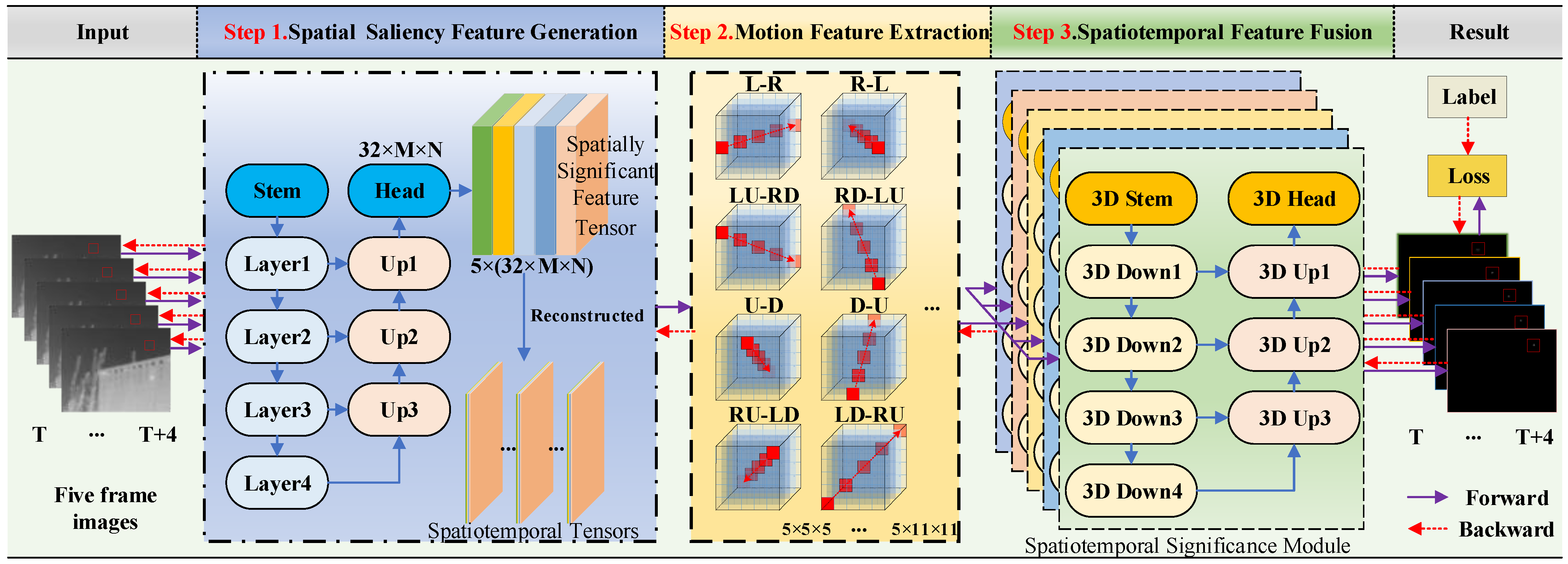
The spatial and temporal dimensions were integrated into a multiframe IRDST detection network. The salient airspace features and time-domain motion characteristics of the target were incorporated into a unified network architecture based on 3D convolution, which achieved multiframe IRDST detection via an end-to-end network.

(2)

According to the consistency of the short-term moving direction of the IRDST, its multiscale three-dimensional motion features with fixed weights were convolved to synchronously enhance the temporal and spatial significance of the target and inhibit random clutter and noise, which improved the detectability of IRDSTs with low SCRs.

(3)

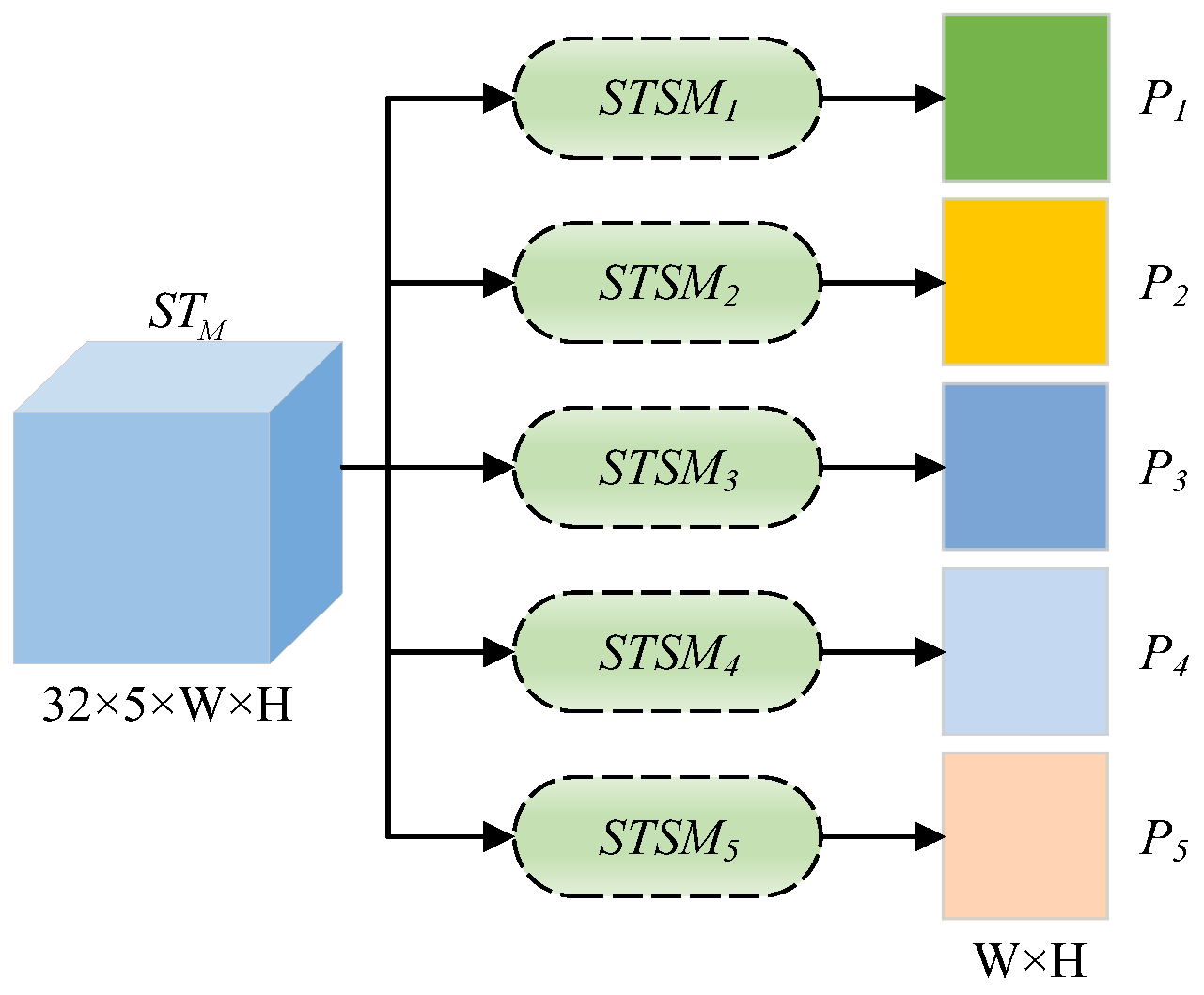
The spatiotemporal characteristics of five parallel and independent optimization strategies were incorporated into the designed spatiotemporal feature fusion-based processing module, which successfully mapped spatiotemporal tensors to target multiframe probability maps.

(4)

Compared with the current methods, the proposed strategy exhibited better detection performance, especially for IRDSTs with low SCRs.

2. Methods

In this section, a spatiotemporally integrated detection network (STIDNet) is realized and applied. First, the main components of the integrated detection network are detailed, the design of the feature extraction layer of the motion saliency and spatiotemporal saliency extraction network is displayed, and the specific implementation of the proposed algorithm under input sequence images is described.

2.1. Overall Architecture

We focus on the design of STIDNet; the network can independently learn the spatiotemporal characteristics of IRDSTs to strengthen its ability to detect IRDSTs with extremely low SCRs. As shown in Figure 2, the overall structure of the network consists of three parts—a spatial saliency feature generation module (SSFGM), a motion feature extraction module (MFEM), and a spatiotemporal feature fusion module (STFFM).

Section 2.2. presents the design of a U-shaped network for extracting the spatial saliency for IRDSTs. Section 2.3. describes the proposed multiscale motion feature-based 3D convolution kernel (FWMFCK-3D) for accumulating the spatial saliency of IRDSTs via a prior motion. Section 2.4. details the mapping from the spatiotemporal motion feature tensor to an IRDST probability. Finally, Section 2.5 and Section 2.6 introduce the loss functions and applications of the network, respectively.

2.2. Spatial Saliency Feature Generation Module

The network input is a sequence of infrared images ${ℝ}^{T\times W\times H}$, where T denotes the length of the input sequence (5 frames are used in the paper), and W and H denote the width and height of the images, respectively. For a single-frame image $I\in {ℝ}^{5\times W\times H}$ in a sequence, a U-shaped network [33] is used as the backbone network to extract the significance of the spatial domain, and the weight parameters of the network are shared by all the images contained in the sequence.

To ensure that the diversity of the spatial features is conducive to the subsequent temporal information mining process, the head structure of the single-frame detection network is modified to expand the number of output channels from 1 to 32. This modification allows for the extraction of spatially significant feature tensors $S_t^{32\times W\times H}$, which are then concatenated in a frame-by-frame manner.

$$S^{5\times 32\times W\times H}=cat[S_1^{32\times W\times H},S_2^{32\times W\times H},S_3^{32\times W\times H},S_4^{32\times W\times H},S_5^{32\times W\times H}]$$

(1)

where $cat[\cdot ]$ denotes the concatenation operator.

The feature tensor $S^{5\times 32\times W\times H}$ is reconstructed as spatiotemporal tensor $S{T}^{32\times 5\times W\times H}$ according to the temporal dimension for the subsequent extraction of temporal motion features.

2.3. Motion Feature Extraction Module

In the infrared search and discovery system, because of the long target distance and the high frame rate of the input image, the speed of the target on the image plane is limited and the direction of the target motion has strong consistency within a short period. According to the above characteristics, we designed FWMFCK-3D to convolve the spatiotemporal tensor $S{T}^{32\times 5\times W\times H}$ and accumulate the spatial significance of IRDSTs according to their prior motion to improve the detectability of IRDSTs with low SCRs.

The eight 3D motion directions are shown in Figure 3; these are left-right, left-up, and right-down; up-down, right-up, and left-down; right-left, right-down, and left-up; and down-up, left-down, and right-up.

To adapt to targets with different motion speeds and scales, convolution kernels with four sizes—5 × 5 × 5, 5 × 7 × 7, 5 × 9 × 9, and 5 × 11 × 11—were designed, and their depth direction was 5. Eight 5 × 5 × 5 convolution kernels are shown in Figure 4. The value of the red pixel is taken to be 1, and the values of the non-red pixels are taken to be 0. The other sizes used for the fixed-weight convolution kernels were set up with reference to the 5 × 5 × 5 dimensions.

Thirty-two 3D convolution kernels with fixed weights are obtained, and they are denoted as follows:

$$\begin{array}{r}3D-FWC{K}^{Di}=cat(FWC{K}_{L-R}^{Di},FWC{K}_{LU-RD}^{Di},FWC{K}_{U-D}^{Di},FWC{K}_{RU-LD}^{Di},\\ FWC{K}_{R-L}^{Di},FWC{K}_{RD-LU}^{Di},FWC{K}_{D-U}^{Di},FWC{K}_{LD-RU}^{Di}) Di\in \left\{5,7,9,11\right\}\end{array}$$

(2)

The padding was set so that the input and output W × H dimensions were consistent, and the spatiotemporal tensor was convolved with $3D-FWC{K}^{Di}$ to obtain a spatiotemporal motion feature tensor $S{T}_M$, as follows:

$$S{T}_M=S{T}^{32\times 5\times W\times H}\ast 3D-FWC{K}^{Di}$$

(3)

As show in Figure 5, $S{T}^{32\times 5\times W\times H}$ was convolved with the convolution kernel at each scale to generate a tensor possessing a size of 8 × 5 × W × H. The size of spatiotemporal motion feature tensor $S{T}_M$ obtained by splicing the tensors at four scales was 32 × 5 × W × H, which is consistent with that of $S{T}^{32\times 5\times W\times H}$.

Ablation experiments were designed to demonstrate the effectiveness of this structure in Section 3.4.

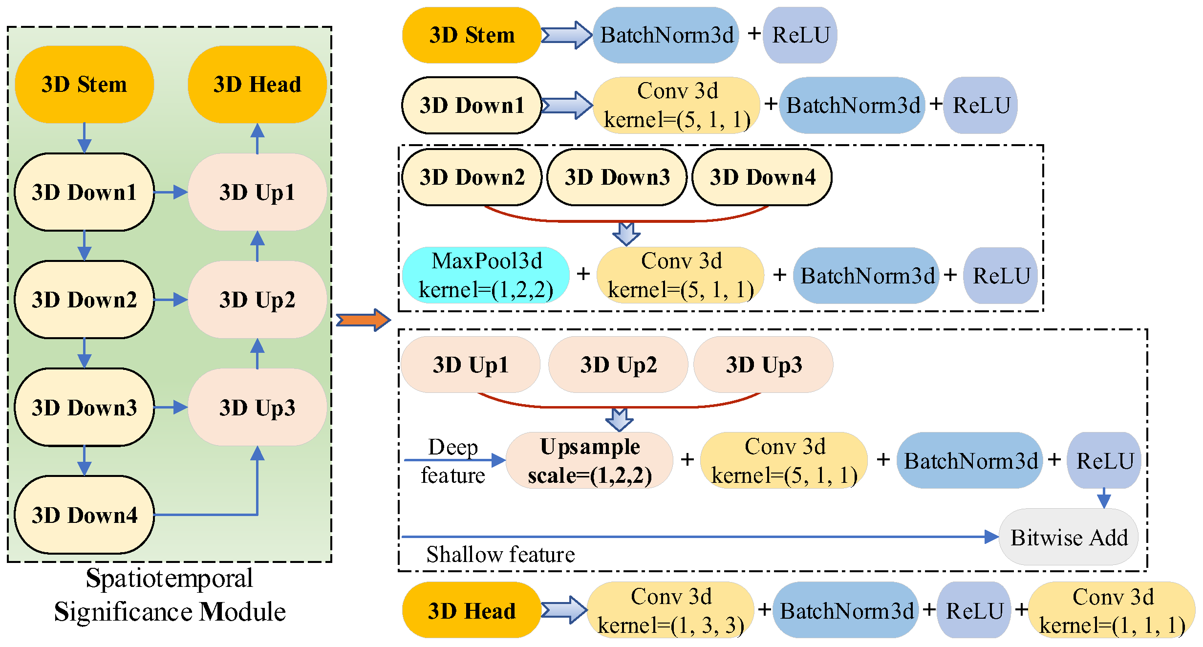
2.4. Spatiotemporal Feature Fusion Module

The STFFM, which is based on 3D convolution, was adopted to map the spatiotemporal motion feature tensor to the probability map of the IRDST. As shown in Figure 6, a U-shaped network was employed in a spatiotemporal significance module (STSM) to better extract and fuse the shallow high-resolution and deep low-resolution feature maps. It used three rounds of up-and-down-sampling to extract features at different scales, and fuses the features with different depths via a cascading approach.

As shown in Figure 7, five STSMs were adopted to map ST_M to the target probability maps of the five frames. The modules operate in parallel with each other and without sharing weights.

$$P=\{P_1,\dots ,P_5\}=\left\{STS{M}_1(S{T}_M),\dots ,STS{M}_5(S{T}_M)\right\} \mathrm{t}\in \left[1,2,3,4,5\right]$$

(4)

where $P$ is the target probability likelihood map generated by STSMs.

2.5. Loss Function

IRDSTD is actually a binary classification problem involving each pixel point of the input image, but since the number of IRDST samples is extremely low in proportion to the background, the numbers of training samples are extremely imbalanced, which leads to slow training convergence. Therefore, the focus loss [34] was chosen as the loss function for the probability map of each image frame to increase the weights of the small number of positive samples and improve the convergence speed of the training process. The sum of the focus losses calculated for 5 image frames is used as the total loss of the network.

$$\begin{array}{l}{\mathrm{FL}}_t(P_t{,\mathrm{y}}_t{)=-\mathrm{y}}_t{\left(1-P_t\right)}^{\gamma }\log (P_t)-\left(1-y_t\right)P_t^{\gamma }\log (1-P_t)\\ Loss={{\displaystyle \sum \mathrm{FL}}}_t t\in [1,2,3,4,5]\end{array}$$

(5)

where ${\mathrm{y}}_t$ is the label, and the value of $\gamma$ is set as 2.

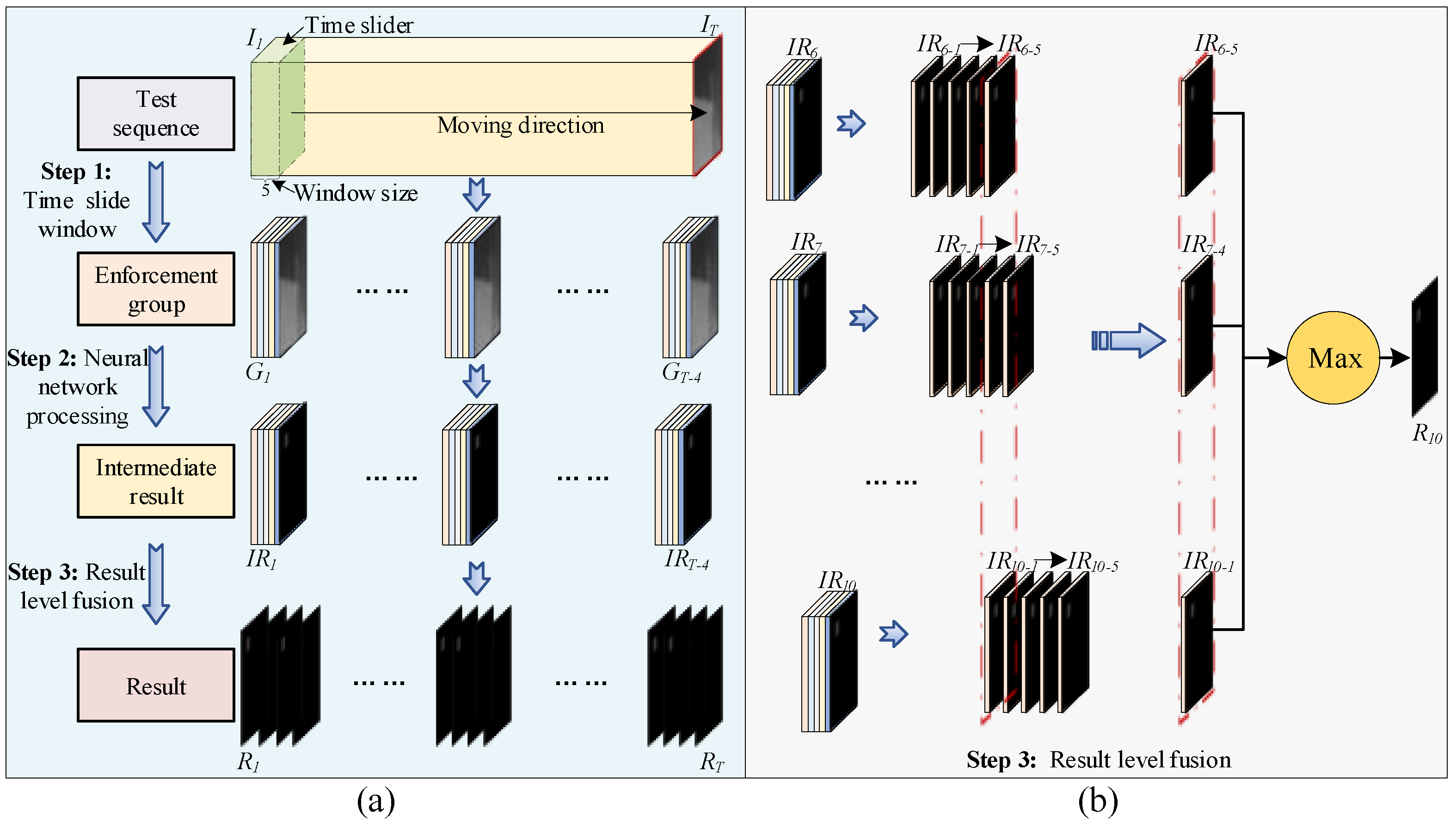
2.6. Result-Level Fusion in the Implementation

The application process for sequence images $I_N^{W\times H}=\left\{I_1^{W\times H},I_2^{W\times H},\dots ,I_T^{W\times H}\right\}$ is shown in Figure 8a.

Step 1: Time slide window

A time slider was used to group the input sequences along the time direction to obtain the following network input:

$$G_N^{5\times W\times H}=\left\{G_1^{5\times W\times H},G_2^{5\times W\times H},\dots ,G_{T-4}^{5\times W\times H}\right\}$$

(6)

where

$$G_1^{5\times W\times H}=\left\{{\mathrm{S}}_1,{\mathrm{S}}_2,{\mathrm{S}}_3,{\mathrm{S}}_4,{\mathrm{S}}_5\right\},\dots ,G_{T-4}^{5\times W\times H}=\left\{{\mathrm{S}}_{T-4},{\mathrm{S}}_{T-3},{\mathrm{S}}_{T-2},{\mathrm{S}}_{T-1},{\mathrm{S}}_T\right\}$$

Step 2: Neural network processing

$G_N^{5\times W\times H}$ was entered into the network to obtain the result $I{R}_N$;

$$I{R}_N=F_{STIDNet}(G_N^{5\times W\times H}) \mathrm{N}\in [1,2,\dots ,T-4]$$

(7)

where $F_{STIDNet}()$ denotes inference using the STIDNet network via the trained weights.

Step 3: Result level fusion

For a frame such as $I_{10}^{W\times H}$ from the input sequence image $I_N^{W\times H}$, as shown in Figure 8b,$I_{10}^{W\times H}$ has 5 detection results in $I{R}_6~I{R}_{10}$, whose inputs are $G_6^{5\times W\times H}~G_{10}^{5\times W\times H}$ $\left(I_6^{W\times H},I_7^{W\times H},\dots ,I_{10}^{W\times H},\dots ,I_{14}^{W\times H}\right)$, so the process of obtaining $R_{10}$ (the final result of $I_{10}^{W\times H}$) via $I{R}_6~I{R}_{10}$ utilized up to 9 image frames, thus using more contextual information.

Specifically, we proposed the result set fusion strategy of the maximum method to obtain the final result, as shown in Figure 8b. The fusion formula is as follows:

$$\begin{gathered} R_K(i,j)=Max[I{R}_{\left(K-4\right)\_5}(i,j),I{R}_{\left(K-3\right)\_4}(i,j),I{R}_{\left(K-2\right)\_3}(i,j), \\ \hspace{1em}\hspace{1em}\hspace{1em}\hspace{1em}\hspace{1em}\hspace{1em}\hspace{1em}\hspace{1em}I{R}_{\left(K-1\right)\_2}(i,j),I{R}_{K\_1}(i,j)] 1\le i\le W,1\le j\le H,1\le K\le T \end{gathered}$$

(8)

where $(i,j)$ is the pixel position, $R_K(i,j)$ is the probability of an IRDST pixel being located at $(i,j)$ in the Kth frame, and $Max[\cdot ]$ is the maximum operation. $I{R}_{\left(K-4\right)\_5}(i,j)$ is the processing result of the network, and $(K-4)\_5$ denotes the 5th frame of the network result obtained for the network input $G_{K-4}^{5\times W\times H}$.

3. Experiments and Results

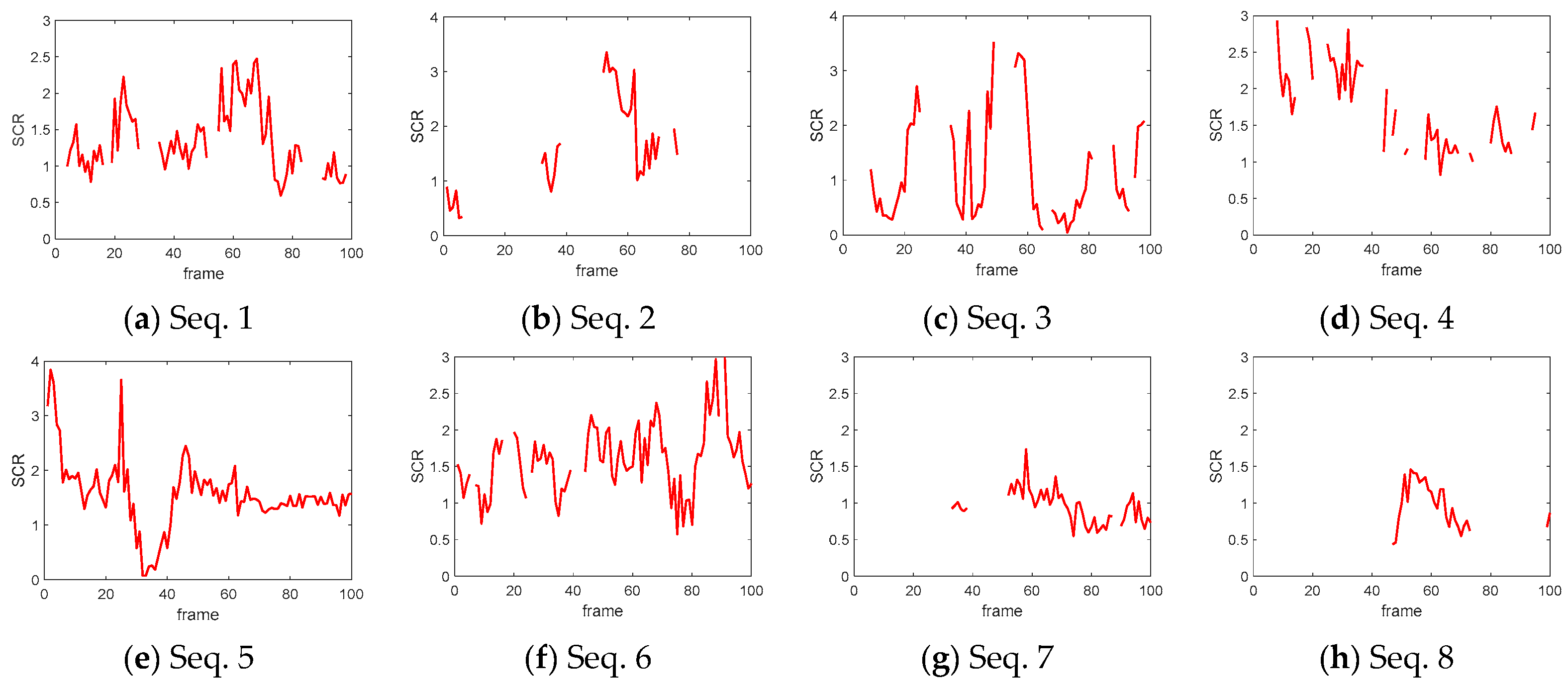
3.1. Dataset

The open-source dataset NUDT-MIRSDT [32] was used as the main training and validation data for the algorithm proposed in this paper.

Training dataset: This dataset included a total of 100 sequences, each containing 100 images, and each sequence constitutes 96 training groups, totaling 9600 training samples.

Test dataset: This dataset included a total of 20 sequences, totaling 1920 test samples.

In the test dataset, the mean SCR of the target across eight sequences is less than 3, making this a typical dim target. As the attention focus related to the data, the SCR change curve is shown in Figure 9.

3.2. Performance Evaluation Indices

Regarding the IRDST detection performance of the proposed approach, the receiver operating characteristic (ROC) curve, which can characterize global performance, and the signal clutter ratio gain (SCRG) and background suppression factor (BSF), which can measure local performance, were used as evaluation indices.

The vertical coordinate of the ROC curve is the true-positive rate (TPR), and the horizontal coordinate is the false-positive rate (FPR). The TPR and FPR measure the classification ability of a model from the perspectives of positive samples and negative samples, respectively. The larger the AUC value is, the stronger the classification ability.

The calculation formulas for the TPR and FPR are as follows:

$$\begin{array}{l}FPR={\displaystyle \frac{FP}{N}}\\ TPR={\displaystyle \frac{TP}{P}}\end{array}$$

(9)

where TP, FP, P, and N represent the number of true positives (correct detections), the number of false positives (false alarms), the total number of positive samples, and the total number of negative samples, respectively. The area under the curve (AUC) is the quantitative index of the ROC curve.

BSF and SCRG are calculated as follows:

$$BSF={\displaystyle \frac{C_{in}}{C_{out}}}$$

(10)

where $C_{in}$ represents the standard deviation of the original infrared image and $C_{out}$ represents the standard deviation of the infrared image processed by the detection algorithm. A larger BSF indicates better background suppression.

$$SCRG={\displaystyle \frac{SC{R}_{\mathrm{o}ut}}{SC{R}_{in}}}$$

(11)

$$SCR={\displaystyle \frac{\left|{\mu }_T-{\mu }_B\right|}{{\sigma }_B}}$$

(12)

where $SC{R}_{\mathrm{o}ut}$ and $SC{R}_{in}$ denote the SCR of the original target and the SCR of the final target, respectively. ${\mu }_T$, ${\mu }_B$, and ${\sigma }_B$ represent the average pixel intensity of the target region, the average pixel intensity of the neighboring region around the target, and the standard deviation of the neighboring region, respectively. $SCRG$ demonstrates the enhancement effect the algorithm attained for the target, and a larger $SCRG$ indicates an algorithmic gain for the IRDST.

3.3. Network Training

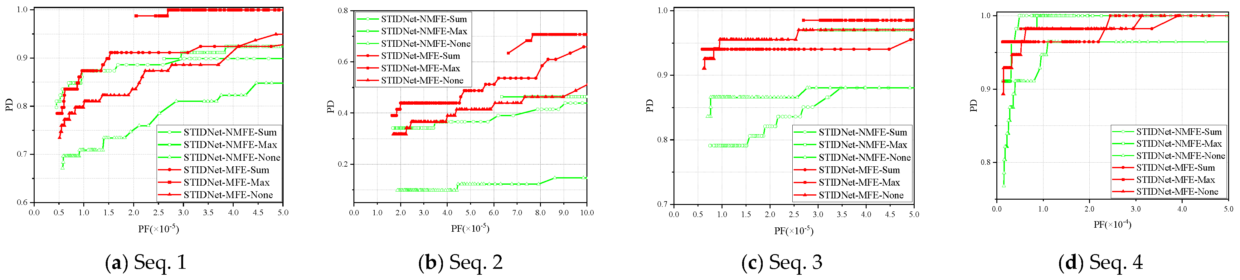
The computer was equipped with an Intel(R) Core (TM) i9-14900K CPU @ 3.20 GHz (Intel Corporation, Santa Clara, United States of America) and an NVIDIA GeForce RTX 4090 GPU @ 24 GB (NVIDIA Corporation, Santa Clara, United States of America). The main software versions were as follows: Python 3.8.16, Pytorch 1.13.1, and Cuda 11.6.1.

Adaptive moment estimation (Adam) was used as the optimizer for training, the initial learning rate was set to 0.001, and the weight attenuation coefficient was set to 0.5. We adopted the ROC optimization method to save the best weights.

$$Best\_weight=\left\{\begin{array}{l}Weigh{t}_{epoch}, if AU{C}_{epoch}\ge best\_AUC\\ Best\_weight, otherwise\end{array}\right.$$

(13)

where $AU{C}_{epoch}$ is the AUC for the dataset in the current epoch. $best\_AUC$ is the historically best AUC. $Weigh{t}_{epoch}$ is the weight for the current epoch. $Best\_weight$ is the historically best weight. If $AU{C}_{epoch}\ge best\_AUC$, we updated the optimal weights.

3.4. Ablation Study

To demonstrate the necessity of the MFEM and the result-level maximum fusion strategy, we designed the following groups for ablation experiments.

The three experimental groups were designated as STIDNet-NMFE-Sum, STIDNet-NMFE-Max, and STIDNet-NMFE-None, with None MFEM. However, they adopted different fusion strategies—Sum, Max, and with None fusion. A comparison of these three experiments may reveal which fusion strategy has advantages.

For the purpose of comparison, the remaining three experimental groups, namely STIDNet-MFE-Sum, STID-Net-MFE-Max, and STIDNet-MFE-None, all utilize the MFEM. This experiment aims to demonstrate the importance of the MFEM in extracting the motion features of IRDST.

The setups of the six groups of ablation experiments are shown in

Table 1. The setup of the ablation experiments.

No.	Methods	Motion Feature Extraction	Fusion Method
1	STIDNet-NMFE-Sum	✘	SUM
2	STIDNet-NMFE-Max	✘	MAX
3	STIDNet-NMFE-None	✘	✘
4	STIDNet-MFE-Sum	✓	SUM
5	STIDNet-MFE-Max	✓	MAX
6	STIDNet-MFE-None	✓	✘

.

The same training data and strategy were used to train the network, and the optimal weights obtained from each group were used to statistically analyze the data with low SCRs (SCR < 3) in the test set. The obtained ROC curves are shown in Figure 10, and the AUC statistics are shown in

Table 2. AUC results in the ablation experimental group.

No.	STIDNet-NMFE-Sum	STIDNet-NMFE-Max	STIDNet-NMFE-None	STIDNet-MFE-Sum	STIDNet-MFE-Max	STIDNet-MFE-None
Seq. 1	0.99906	0.99916	0.99907	0.99921	0.99921	0.99916
Seq. 2	0.95076	0.96522	0.92476	0.99832	0.99904	0.9945
Seq. 3	0.99909	0.99906	0.99889	0.99912	0.99912	0.99913
Seq. 4	0.99878	0.99876	0.99866	0.99877	0.99876	0.99878
Seq. 5	0.99885	0.99885	0.99885	0.99885	0.99885	0.99885
Seq. 6	0.99849	0.99881	0.99871	0.99889	0.99888	0.99889
Seq. 7	0.99931	0.9993	0.99931	0.99931	0.9993	0.99931
Seq. 8	0.9653	0.9695	0.94587	0.98699	0.98974	0.9888
Mean	0.988705	0.9910825	0.983015	0.9974325	0.9978625	0.9971775

.

(1) Evaluation of MFEM’s effect on IRDSTD performance

Under the same fusion method, the ROC curves and AUCs produced with and without MFEM were compared. From a qualitative perspective, as shown in Figure 10, the ROC curves of the experimental groups that employed MFEM (red) were, in general, superior to those that did not (green), as evidenced by their location in the upper left corner of the axis. From a quantitative perspective, the AUC enhancement of 0.0087/0.0068/0.0142 for a IRDST (SCR < 3) was achieved with the employed of MFEM by comparing STID-Net-MFE-Sum with STID-Net-NMFE-Sum, STID-Net-MFE-Max with STID-Net-NMFE-Max, and STID-Net-MFE-None with STID-Net-NMFE-None. This is attributable to the utilization of a priori information gathering energy from the motion of a IRDST with a low SCR using MFEM, thereby enhancing the distinction between the targets and clutter, and achieving a higher AUC.

(2) Evaluation of maximal fusion strategy effect on IRDSTD performance

The influence of the fusion strategy on the resulting performance was analyzed on the premise of ensuring the consistency of the motion feature extraction settings. The ROC curves and average AUCs of STIDNet-MFE-Max and STIDNet-MFE-Sum were better than those of STIDNet-MFE-None, which indicated that the performance of fusion processing was superior to that of non-fusion processing. This was due to the fact that the fusion strategy employs a greater quantity of contextual information for IRDSTD.

In particular, by comparing STIDNet-MFE-Max and STIDNet-MFE-Sum, as well as STIDNet-MFE-Max and STIDNet-MFE-None, the AUC values increased by 0.0023/0.0080, respectively. In the experimental group utilizing the MFEM, the AUC was also enhanced by 0.00043/0.00068 through the implementation of the maximum fusion strategy.

The above analysis results can be described as follows.

(1)

The AUC achieved on the test set by the network with motion feature extraction was better than that of the network without motion feature extraction. Motion feature extraction can significantly improve the ability to detect IRDSTs.

(2)

Fusion processing was superior to non-fusion processing. After conducting a comparison, the AUC of the maximum value fusion method was the highest.

Hence, in the subsequent comparative experiments with other methods, STIDNet-MFE-Max was adopted as the optimal version of the algorithm proposed in this work.

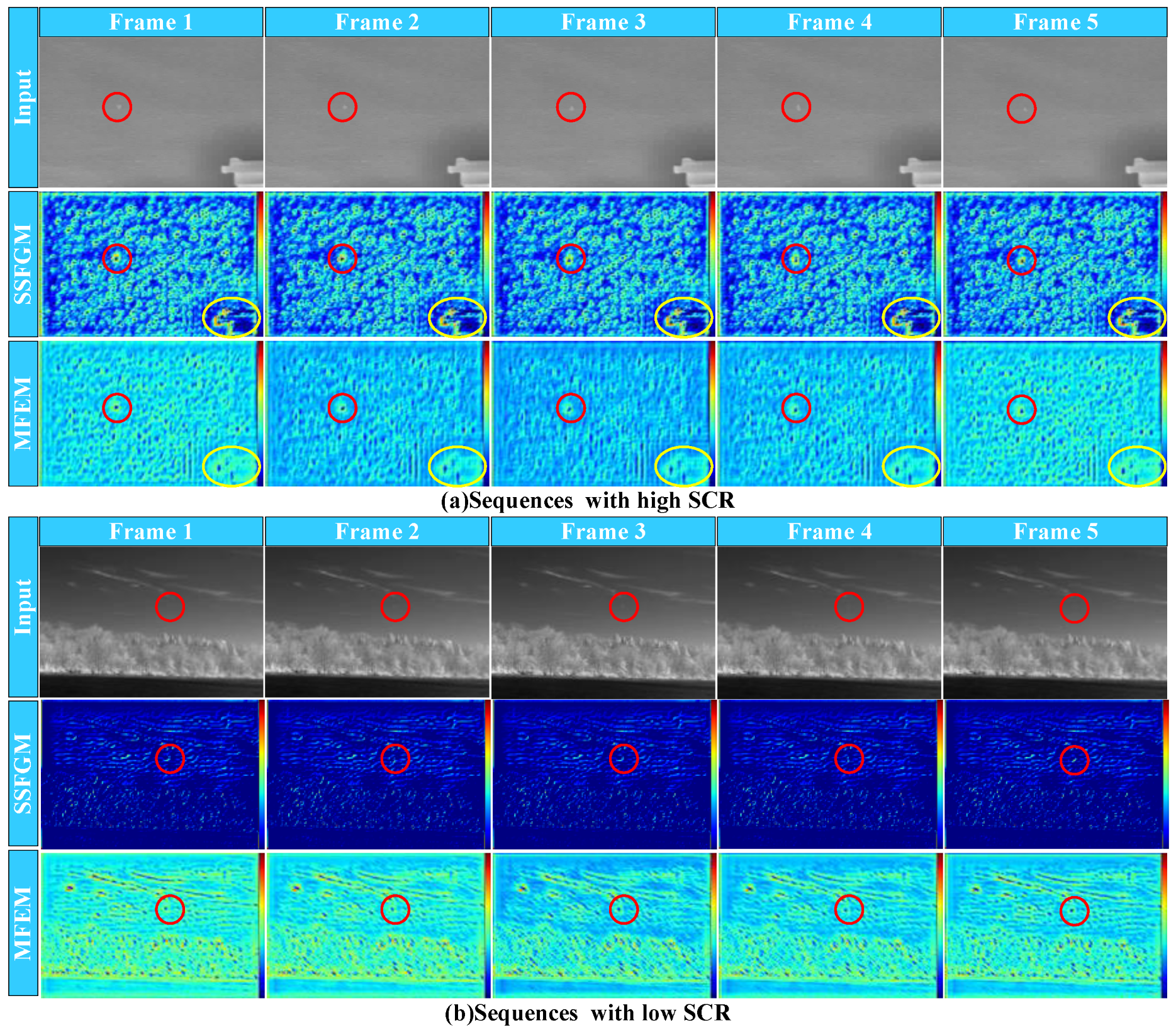
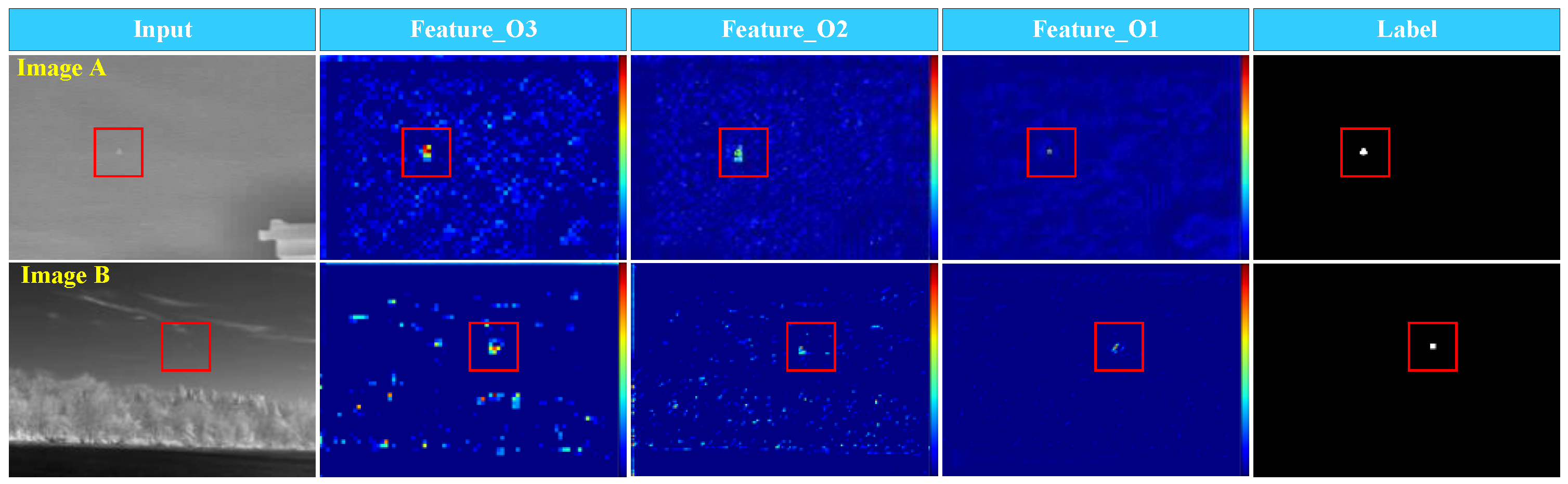
3.5. Visual Analysis of Feature Maps

(1) Visualization of MFEM’s usefulness

The following discussion attempted to provide a visual representation of the benefits of MFEM. A visual analysis was performed via the feature maps produced before and after the application of the MFEM, as shown in Figure 11.

As shown in Figure 11a, strong responses were observed for the target and lower-right building areas when utilizing the SSFGM without the MFEM. However, strong clutter was significantly attenuated at the edge of the building after the MFEM was applied. This was due to the fact that MFEM possessed the effect of enhancing the saliency of the moving IRDST, while the edge of the building was stationary and was thus suppressed after MFEM was applied.

Furthermore, as shown in Figure 11b, a weak target response was found in the results of the SSFGM, with incomplete extracted target edge features. After applying the MFEM, the target was completely and accurately extracted, which benefited the accumulation of information from multiple frames.

These results indicate that the MFEM can both effectively suppress false alarms and enhance target features.

(2) Visualization of STFFM ’s usefulness

Furthermore, as demonstrated in Figure 12, the efficacy of the STFFM was evidently substantiated.

Feature_O3, Feature_O2, and Feature_O1 represented the deepest, middle, and shallowest features of the upsampled outputs derived from the decoder in the STFFM, respectively.

As the feature map was decoded in a layer-by-layer manner within the network, the response of the target area became increasingly focused, whereas that of the background and clutter weakened. This was because the encoding and decoding of spatiotemporal feature maps was carried out in the STFFM, which accumulated the spatial energy of the IRDSTs in the time dimension, thereby significantly enhancing the saliency of the IRDST.

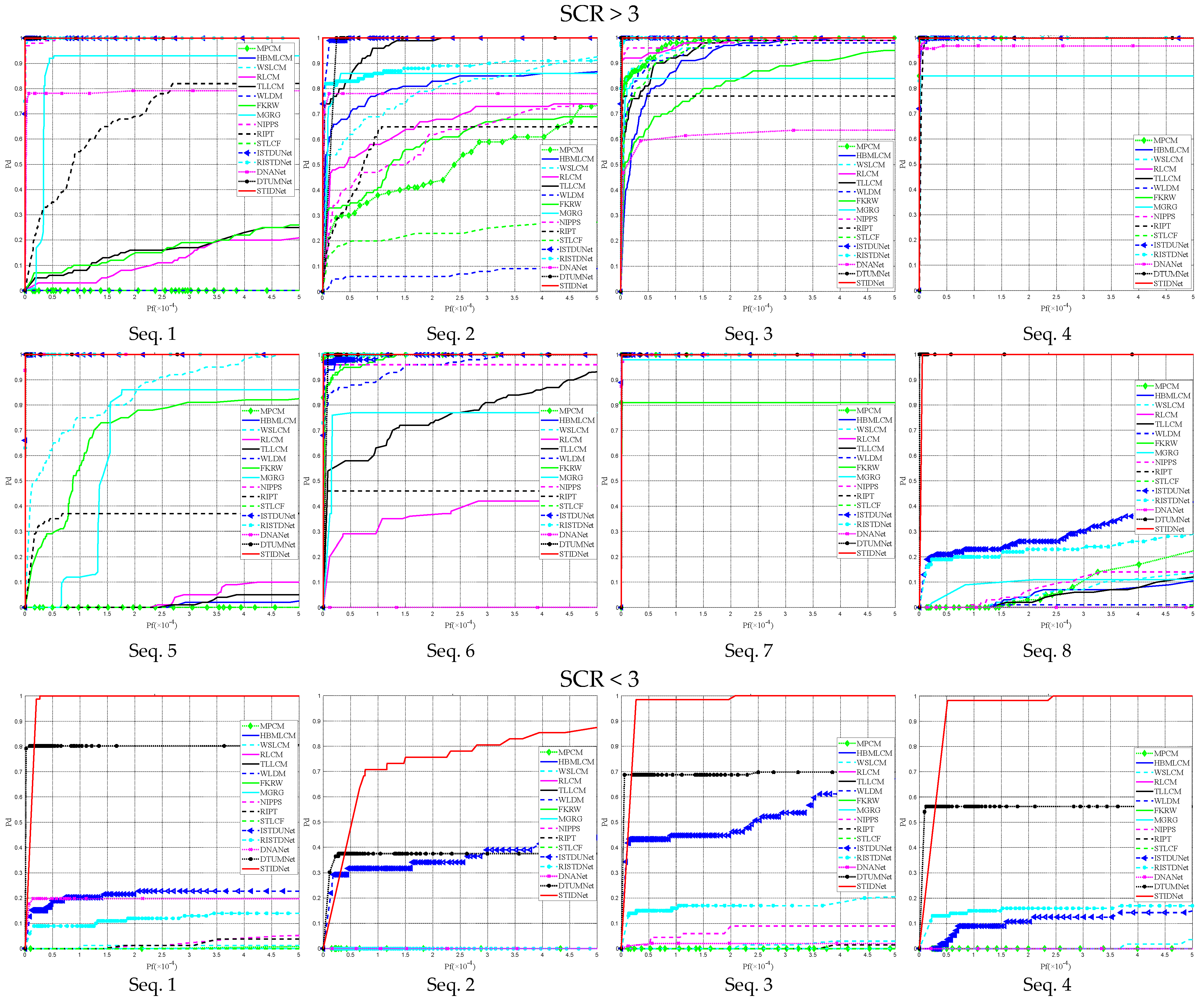
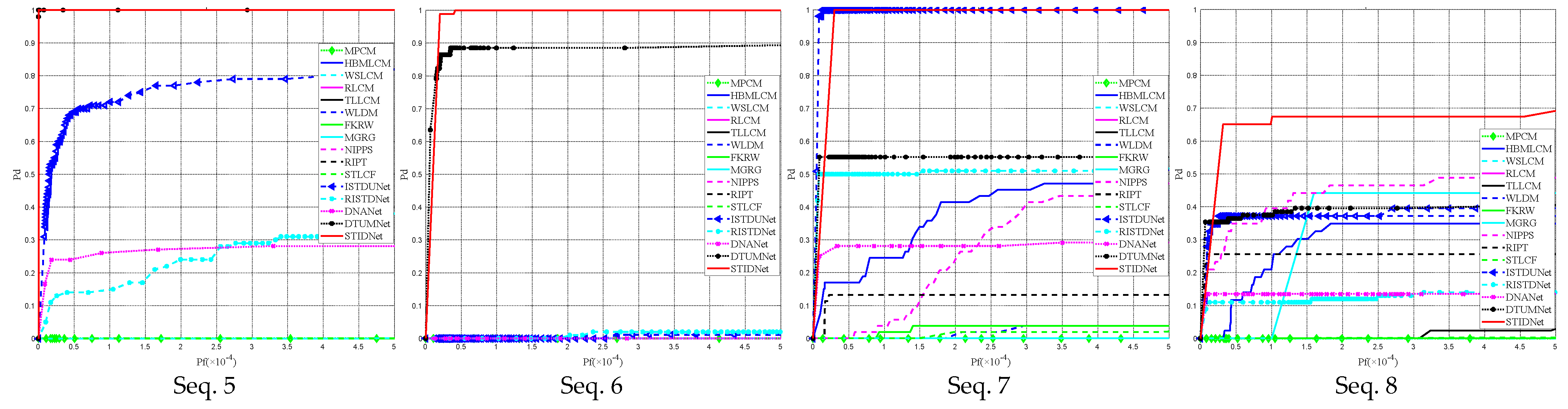
3.6. Comparison Experiments

To explore the performance of the method developed in this work, we compared it with the state-of-the-art IRDSTD methods, including traditional methods (MPCM, HBMLCM, WSLCM, RLCM, TLLCM, NIPPS, RIPT, WLDM, FKRW, MGRG, and STLCF) and methods based on deep learning (ISTDUNet, RISTDNet, DNANet, and DTUMNet). All the traditional methods used their default parameters, and the methods based on deep learning were retrained on the dataset to obtain the optimal weights. The specific parameter settings of the algorithms, the FPS results, and the parameters of the deep learning algorithms are shown in

Table 3. Parameterization of the contrast method.

Methods	Publication	Parameter Settings	Params (M)	FPS
MPCM [10]	Pattern Recognit. 2016	L = 3; Window size = [3, 5, 7, 9]	-	36.331
HBMLCM [35]	IEEE Geosci. Remote Sens. Lett. 2018	External window size = 15 × 15; target size = [3, 5, 7, 9]	-	126.098
WSLCM [36]	IEEE Geosci. Remote Sens. Lett. 2021	Gauss_krl = [1, 2, 1; 2, 4, 2; 1, 2, 1]./16; Scs = [5, 7, 9, 11]	-	0.801
RLCM [11]	IEEE Geosci. Remote. Sens. Lett. 2018	Scale = 3; k1 = [2, 5, 9]; k2 = [4, 9, 16]	-	1.024
TLLCM [13]	IEEE Geosci. Remote. Sens. Lett. 2019	GS = [1/16, 1/8, 1/16; 1/8, 1/4, 1/8; 1/16, 1/8, 1/16]	-	1.533
NIPPS [15]	Infr. Phys. Technol. 2017	PatchSize = 50; SlideStep = 10; LambdaL = 2; RatioN = 0.005	-	0.249
RIPT [16]	IEEE J. Sel. Topics Appl. Earth Observ. Remote Sens. 2017	PatchSize = 30; SlideStep = 10; LambdaL = 0.7; MuCoef = 5; h = 1	-	1.238
WLDM [37]	IEEE Trans. Geosci. Remote Sens. 2016	L = 9	-	0.389
FKRW [38]	IEEE Trans. Geosci. Remote Sens. 2019	L = [−4, −1, 0, −1, −4; −1, 2, 3, 2, −1; 0, 3, 4, 3, 0;−1, 2, 3, 2, −1; −4, −1, 0, −1, −4]	-	9.034
MGRG [39]	IEEE Geosci. Remote. Sens. Lett. 2019	numSeeds = 20; tarRate = 0.01 × 0.15	-	1.422
STLCF [25]	Computers and Electrical Engineering. 2018	tspan_rng = 2; swind_rng = 7	-	2.749
ISTDUNet [33]	IEEE Trans. Geosci. Remote Sens. Lett. 2022	hyperparameter of channel = 2	2.761	23.027
RISTDNet [17]	IEEE Trans. Geosci. Remote Sens. Lett. 2022	-	0.763	4.723
DNANet [19]	IEEE Trans. Image Process. 2023	-	1.134	20.747
DTUMNet [32]	IEEE Trans. on Neural Networks and Learning Systems. 2023	Res-Unet	0.298	9.494
STIDNet	-	-	4.874	5.945

.

As shown in Figure 13., the performance of the proposed approach was compared with that of other algorithms, and the ROC curves are described as follows.

As evidenced by the ROC curves, deep learning consistently exhibited superior performance in comparison to traditional methods, particularly in scenarios where targets had low signal-to-noise ratios. The ROC curves of the other algorithms were obviously biased toward the lower-right corner of the coordinate axis, whereas those of the proposed algorithm were all in the upper-left corner of the coordinate system, particularly for low-SCR targets, indicating its excellent detection ability.

The AUCs of the ROC curves are illustrated as the quantitative analysis results in

Table 4. AUC results of comparative experiments.

Seq.		WSLCM	RLCM	TLLCM	NIPPS	RIPT	STLCF	ISTDUNet	RISTDNet	DNANet	DTUMNet	STIDNet
S C R > 3	1	0.9987	0.9972	0.9979	0.9987	0.9087	0.9833	0.9987	0.9987	0.9727	0.9987	0.99865
	2	0.9689	0.9713	0.9990	0.8690	0.8241	0.9926	0.9990	0.9972	0.9890	0.9990	0.99901
	3	0.9989	0.9989	0.9989	0.9939	0.8840	0.9989	0.9989	0.9989	0.9775	0.9989	0.9989
	4	0.9989	0.9989	0.9989	0.9989	0.9989	0.9989	0.9989	0.9989	0.9984	0.9989	0.99885
	5	0.9981	0.9933	0.9965	0.9982	0.6837	0.9844	0.9982	0.9982	0.9982	0.9982	0.9982
	6	0.9987	0.9930	0.9985	0.9787	0.7290	0.9987	0.9987	0.9987	0.5054	0.9987	0.99866
	7	0.9990	0.9936	0.9990	0.9990	0.9990	0.9990	0.9990	0.9990	0.9990	0.9990	0.99903
	8	0.9501	0.9577	0.9957	0.5691	0.4993	0.9823	0.9954	0.9641	0.7676	0.9987	0.99873
	9	0.9881	0.9959	0.9981	0.9426	0.4994	0.9871	0.9987	0.9983	0.9362	0.9989	0.99889
	10	0.9982	0.9959	0.9983	0.9979	0.5940	0.9952	0.9984	0.9985	0.4848	0.9985	0.99845
	11	0.9780	0.9249	0.9983	0.8885	0.6490	0.9965	0.9985	0.9978	0.9438	0.9985	0.99853
	12	0.9990	0.9989	0.9990	0.9989	0.9989	0.9983	0.9990	0.9990	0.9989	0.9989	0.99895
	Mean	0.98955	0.98496	0.99818	0.93612	0.77233	0.99293	0.99845	0.99561	0.88096	0.99874	0.99874
S C R < 3	1	0.51761	0.50963	0.87721	0.72535	0.51833	0.97573	0.95366	0.7933	0.78389	0.98842	0.99921
	2	0.5213	0.7861	0.9832	0.4996	0.4993	0.7348	0.9933	0.5819	0.4579	0.7737	0.99904
	3	0.5505	0.5343	0.8537	0.5589	0.5509	0.8941	0.9962	0.9319	0.6491	0.9834	0.99912
	4	0.5436	0.4658	0.8897	0.4994	0.4989	0.6392	0.9900	0.8321	0.5795	0.9053	0.99876
	5	0.5274	0.5913	0.9778	0.6923	0.4981	0.7893	0.9979	0.9772	0.8919	0.9989	0.99885
	6	0.5042	0.4859	0.9244	0.5091	0.4993	0.8581	0.9833	0.9037	0.6659	0.9975	0.99888
	7	0.4992	0.4780	0.5788	0.7351	0.5656	0.9789	0.9993	0.8576	0.7410	0.8156	0.9993
	8	0.4989	0.7642	0.9202	0.7658	0.6277	0.9287	0.9217	0.7248	0.8154	0.9285	0.98974
	Mean	0.52034	0.57690	0.87563	0.62319	0.53227	0.84985	0.97942	0.82531	0.69807	0.92392	0.99786

.

Compared with the other algorithms, the proposed method achieved the best performance when the SCR > 3. Moreover, when SCR < 3, the mean AUC value attained for eight sequences still reached 0.99786, indicating a significant advantage. The ROC curve and AUC results indicate that the developed algorithm has an excellent performance, particularly for IRDSTs with low SCRs.

Moreover, the performance differences observed between this algorithm and the other state-of-the-art methods in the local areas of small and dim targets are displayed in

Table 5. BSF results of comparative experiments. The best results are in red; the second-best results are in blue; and the third-best results are in green.

Seq.		WSLCM	RLCM	TLLCM	NIPPS	RIPT	STLCF	ISTDUNet	RISTDNet	DNANet	DTUMNet	STIDNet
S C R > 3	1	38.6	5.6	9.14	278.3	32.5	2.1	1358.4	278.3	5.7	1365.3	2251.7
	2	988.5	7.2	9.59	524.6	1860.2	2.9	240.3	47.6	1.3	588.3	1711.0
	3	2109.6	15.4	64.0	257.9	1046.1	5.9	746.3	204.1	7.1	795.7	1848.9
	4	20.3	3.0	6.4	11.2	8.1	2.3	52.4	8.4	2.7	1300.9	1557.6
	5	14.2	1.4	2.6	15.2	19.5	1.3	13.7	11.5	0.9	529.6	935.2
	6	18.5	3.4	6.8	11.0	24.3	2.2	43.5	39.4	1.6	534.5	1484.5
	7	23.1	1.3	3.4	6.4	9.8	1.1	8.1	14.9	0.3	196.0	410.6
	8	13.7	1.3	2.3	7.3	619.7	1.4	52.4	21.2	0.6	509.5	598.9
	9	688.2	5.3	14.5	55.1	28.6	2.1	589.5	114.6	3.0	652.3	1131.9
	10	28.7	10.3	21.9	17.8	28.4	4.3	44.2	14.3	8.3	1392.9	2205.1
	11	21.0	6.2	10.5	35.1	55.0	1.8	765.7	340.9	4.2	630.0	1814.0
	12	2.8	2.3	2.3	37.1	82.6	1.2	126.5	29.9	8.1	467.4	1445.0
S C R < 3	1	25.5	4.9	26.4	51.0	46.4	2.6	33.5	12.5	4.9	708.6	1163.0
	2	22.5	8.0	9.3	42.2	20.5	1.4	147.9	29.2	5.2	1910.9	887.6
	3	22.2	4.0	5.6	17.5	7.2	1.6	56.6	31.0	1.4	501.0	1045.2
	4	15.1	2.7	6.9	24.5	6.4	1.5	13.0	16.1	1.8	965.8	1164.4
	5	137.5	2.1	3.3	39.0	8.7	1.4	96.7	11.1	1.6	352.3	545.8
	6	84.7	8.7	16.5	32.1	26.5	2.1	204.6	27.3	4.4	487.7	1768.7
	7	104.9	4.7	6.7	74.7	622.7	2.3	414.8	74.7	3.6	857.6	1687.2
	8	1054.4	6.0	12.7	85.8	38.9	2.2	624.2	502.9	4.1	1341.5	1629.2

and

Table 6. SCRG results of comparative experiments. The best results are in red; the second-best results are in blue; and the third-best results are in green.

Seq.		WSLCM	RLCM	TLLCM	NIPPS	RIPT	STLCF	ISTDUNet	RISTDNet	DNANet	DTUMNet	STIDNet
S C R > 3	1	1313.7	1.0	277.2	1518.3	614.1	3.4	578.4	24.9	1.1	1022.4	1241.5
	2	2194.1	1.5	1492.1	1746.6	951.8	2.4	68.9	5.3	0.1	659.4	1127.2
	3	2806.6	1.6	1718.9	1239.0	1391	4.0	919.3	1053.9	1.8	1133.9	1817.0
	4	0.0	0.3	182.7	14.8	0.0	5.8	256.8	88.0	2.3	9490.6	6081.9
	5	45.9	1.4	3.5	16.4	0.0	1.2	33.9	8.6	0.3	1430.9	1620.5
	6	753.0	1.4	819.3	190.1	0.0	1.3	4.4	5.5	0.2	438.7	221.8
	7	535.6	1.2	882.4	61.6	26.1	1.0	8.3	4.5	0.1	422.4	203.1
	8	793.9	0.7	1352.1	918.6	421.3	1.6	27.9	14.1	0.2	1141.4	651.4
	9	1664.2	1.2	149.6	1107.8	1235	2.2	417.1	56.0	1.0	1004.7	1381.4
	10	0.4	0.1	7.1	5.2	0.0	2.0	6.0	28.2	0.7	5321.5	2736.5
	11	0.0	0.1	145.3	666.2	633.2	4.3	683.0	215.7	3.0	2859.4	2466.1
	12	0.0	0.0	232214	58.0	1571	1412.7	25336.6	18766.9	2130.7	7416719	398266
S C R < 3	1	20.8	0.6	12.3	18.8	5.0	2.9	131.9	39.9	0.8	3263.6	3281.2
	2	0.8	0.8	2.9	0.0	0.0	1.1	251.7	1.1	1.1	6947.3	4837.8
	3	6.6	0.6	18.1	231.9	141.4	3.1	360.2	73.3	1.6	4968.6	10788
	4	1.5	0.00	36.0	0.0	0.0	2.1	16.5	6.6	0.6	4408.6	4652.2
	5	1094.3	0.8	27.7	1085.5	549.2	1.4	20.6	15.3	0.7	593.1	847.8
	6	832.5	1.6	112.5	485.3	789.3	1.2	65.0	105.0	0.9	454.4	1340.9
	7	1275.7	1.1	23.8	890.2	961.4	1.3	64.8	89.0	0.6	715.6	566.5
	8	1440.6	0.9	68.4	1053.6	1117.3	2.1	72.4	487.7	1.0	1235.3	1101.9

. The BSF and SCRG results indicate that the proposed method is at the leading level among the compared algorithms.

Typical processing results obtained for eight input images are displayed in Figure 14 to observe the detection capabilities of the tested algorithms.

Both the targets from Image 1 and Image 2, which had high SCRs, were successfully detected by all six listed algorithms. However, NIPPS, STLCF, and RISTDNet failed to detect the targets in Image 3–Image 8 because of their low SCRs. The targets in Image 3, Image 4, and Image 7 could be detected by ISTDUNet, whereas the targets in Image 5, Image 6, and Image 8 were not detected. Although DTUMNet successfully detected all the targets, false alarms occurred in Image 4 and Image 8. In the Image 2, Image 3, Image 5, and Image 7 results of DTUMNet, the targets were split into multiple regions and had no integrity, so this approach had difficulty in terms of accurately localizing the target.

Compared with these methods, the proposed method successfully detected all the targets without false alarms, and the detection results were centralized rather than dispersed, implying its satisfactory detection ability.

Furthermore, Figure 15 visualizes the results produced by the algorithm for the sequence images, where the targets were all accurately detected with low SCRs and no false alarms.

4. Conclusions

In this work, spatial saliency and temporal motion feature extraction were incorporated into a unified network architecture via an end-to-end design to construct a spatiotemporally integrated network for the detection of IRDSTs. According to the transcendental motion paradigm, the spatial saliency of the IRDST of interest was accumulated through an FWMFCK-3D model. The FWMFCK-3D model employed a fixed-weight convolutional kernel with eight directions and four scales to aggregate energy from IRDSTs. During spatiotemporal feature fusion processing, the feature tensor was mapped to the probability of the IRDST to detect the target via 3D convolution. In the ablation experiments, the AUC enhancement of 0.0087/0.0068/0.0142 for the IRDST (SCR < 3) was achieved with the FWMFCK-3D module in comparison with the results when the FWMFCK-3D module was not used. The implementation of a maximal fusion strategy resulted in the augmentation of the AUC by 0.0023/0.0080 and 0.00043/0.00068, in comparison to the summation and no fusion methodologies, respectively. Compared with other algorithms, the proposed algorithm presented the best ROC curves, AUCs, and BSFs on the NUDT-MIRSDT dataset, especially for IRDSTs with a SCR < 3, the average AUC value still reached 0.99786.

References

1. Kim, S.; Lee, J. Scale invariant small target detection by optimizing signal-to-clutter ratio in heterogeneous background for infrared search and track. Pattern Recognit. 2012, 45, 393–406. [Google Scholar] [CrossRef]
2. Zhao, M.J.; Li, W.; Li, L.; Hu, J.; Ma, P.G.; Tao, R. Single-Frame Infrared Small-Target Detection: A Survey. IEEE Geosci. Remote Sens. Mag. 2022, 10, 87–119. [Google Scholar] [CrossRef]
3. Deshpande, S.D.; Er, M.H.; Ronda, V.; Chan, P. Max-Mean and Max-Median filters for detection of small-targets. In Proceedings of the Signal and Data Processing of Small Targets, SPIE’s International Symposium on Optical Science Engineering, and Instrumentation, Denver, CO, USA, 4 October 1999; pp. 74–83. [Google Scholar]
4. Han, J.H.; Liu, S.B.; Qin, G.; Zhao, Q.; Zhang, H.H.; Li, N.N. A Local Contrast Method Combined With Adaptive Background Estimation for Infrared Small Target Detection. IEEE Geosci. Remote Sens. Lett. 2019, 16, 1442–1446. [Google Scholar] [CrossRef]
5. Bae, T.W.; Lee, S.H.; Sohng, K.I. Small target detection using the Bilateral Filter based on Target Similarity Index. IEICE Electron. Expr. 2010, 7, 589–595. [Google Scholar] [CrossRef]
6. Bai, X.Z.; Zhou, F.G. Analysis of new top-hat transformation and the application for infrared dim small target detection. Pattern Recognit. 2010, 43, 2145–2156. [Google Scholar] [CrossRef]
7. Zhang, S.F.; Huang, X.H.; Wang, M. Background Suppression Algorithm for Infrared Images Based on Robinson Guard Filter. In Proceedings of the 2nd International Conference on Multimedia and Image Processing (ICMIP), Wuhan, China, 17–19 March 2017; IEEE: New York, NY, USA, 2017; pp. 250–254. [Google Scholar]
8. Chen, C.L.P.; Li, H.; Wei, Y.T.; Xia, T.; Tang, Y.Y. A Local Contrast Method for Small Infrared Target Detection. IEEE Trans. Geosci. Remote Sens. 2014, 52, 574–581. [Google Scholar] [CrossRef]
9. Han, J.H.; Ma, Y.; Zhou, B.; Fan, F.; Liang, K.; Fang, Y. A Robust Infrared Small Target Detection Algorithm Based on Human Visual System. IEEE Geosci. Remote Sens. Lett. 2014, 11, 2168–2172. [Google Scholar] [CrossRef]
10. Wei, Y.T.; You, X.G.; Li, H. Multiscale patch-based contrast measure for small infrared target detection. Pattern Recognit. 2016, 58, 216–226. [Google Scholar] [CrossRef]
11. Han, J.H.; Liang, K.; Zhou, B.; Zhu, X.Y.; Zhao, J.; Zhao, L.L. Infrared Small Target Detection Utilizing the Multiscale Relative Local Contrast Measure. IEEE Geosci. Remote Sens. Lett. 2018, 15, 612–616. [Google Scholar] [CrossRef]
12. Yao, S.K.; Chang, Y.; Qin, X.J. A Coarse-to-Fine Method for Infrared Small Target Detection. IEEE Geosci. Remote Sens. Lett. 2019, 16, 256–260. [Google Scholar] [CrossRef]
13. Han, J.H.; Moradi, S.; Faramarzi, I.; Liu, C.Y.; Zhang, H.H.; Zhao, Q. A Local Contrast Method for Infrared Small-Target Detection Utilizing a Tri-Layer Window. IEEE Geosci. Remote Sens. Lett. 2020, 17, 1822–1826. [Google Scholar] [CrossRef]
14. Gao, C.; Meng, D.; Yang, Y.; Wang, Y.; Zhou, X.; Hauptmann, A.G. Infrared patch-image model for small target detection in a single image. IEEE Trans Image Process. 2013, 22, 4996–5009. [Google Scholar] [CrossRef] [PubMed]
15. Dai, Y.M.; Wu, Y.Q.; Song, Y.; Guo, J. Non-negative infrared patch-image model: Robust target-background separation via partial sum minimization of singular values. Infrared Phys. Technol. 2017, 81, 182–194. [Google Scholar] [CrossRef]
16. Dai, Y.M.; Wu, Y.Q. Reweighted Infrared Patch-Tensor Model With Both Nonlocal and Local Priors for Single-Frame Small Target Detection. IEEE J. Sel. Top. Appl. Earth Obs. Remote Sens. 2017, 10, 3752–3767. [Google Scholar] [CrossRef]
17. Hou, Q.Y.; Wang, Z.P.; Tan, F.J.; Zhao, Y.; Zheng, H.L.; Zhang, W. RISTDnet: Robust Infrared Small Target Detection Network. IEEE Geosci. Remote Sens. Lett. 2022, 19. [Google Scholar] [CrossRef]
18. Tong, X.Z.; Sun, B.; Wei, J.Y.; Zuo, Z.; Su, S.J. EAAU-Net: Enhanced Asymmetric Attention U-Net for Infrared Small Target Detection. Remote Sens. 2021, 13, 3200. [Google Scholar] [CrossRef]
19. Li, B.Y.; Xiao, C.; Wang, L.G.; Wang, Y.Q.; Lin, Z.P.; Li, M.; An, W.; Guo, Y.L. Dense Nested Attention Network for Infrared Small Target Detection. IEEE Trans. Image Process. 2023, 32, 1745–1758. [Google Scholar] [CrossRef]
20. Dai, Y.M.; Wu, Y.Q.; Zhou, F.; Barnard, K. Attentional Local Contrast Networks for Infrared Small Target Detection. IEEE Trans. Geosci. Remote Sens. 2021, 59, 9813–9824. [Google Scholar] [CrossRef]
21. Zuo, Z.; Tong, X.Z.; Wei, J.Y.; Su, S.J.; Wu, P.; Guo, R.Z.; Sun, B. AFFPN: Attention Fusion Feature Pyramid Network for Small Infrared Target Detection. Remote Sens. 2022, 14, 3412. [Google Scholar] [CrossRef]
22. Wang, K.W.; Du, S.Y.; Liu, C.X.; Cao, Z.G. Interior Attention-Aware Network for Infrared Small Target Detection. IEEE Trans. Geosci. Remote Sens. 2022, 60, 5002013. [Google Scholar] [CrossRef]
23. Wu, X.; Hong, D.F.; Chanussot, J. UIU-Net: U-Net in U-Net for Infrared Small Object Detection. IEEE Trans. Image Process. 2023, 32, 364–376. [Google Scholar] [CrossRef] [PubMed]
24. Deng, L.Z.; Zhu, H.; Tao, C.; Wei, Y.T. Infrared moving point target detection based on spatial-temporal local contrast filter. Infrared Phys. Technol. 2016, 76, 168–173. [Google Scholar] [CrossRef]
25. Zhu, H.; Guan, Y.S.; Deng, L.Z.; Li, Y.S.; Li, Y.J. Infrared moving point target detection based on an anisotropic spatial-temporal fourth-order diffusion filter. Comput. Electr. Eng. 2018, 68, 550–556. [Google Scholar] [CrossRef]
26. Sun, Y.; Yang, J.G.; An, W. Infrared Dim and Small Target Detection via Multiple Subspace Learning and Spatial-Temporal Patch-Tensor Model. IEEE Trans. Geosci. Remote Sens. 2021, 59, 3737–3752. [Google Scholar] [CrossRef]
27. Wojke, N.; Bewley, A.; Paulus, D. Simple Online and Realtime Tracking with a Deep Association Metric. In Proceedings of the 24th IEEE International Conference on Image Processing (ICIP), Beijing, China, 17–20 September 2017; IEEE: New York, NY, USA, 2017; pp. 3645–3649. [Google Scholar]
28. Zhang, T.; Zhao, D.F.; Chen, Y.S.; Zhang, H.L.; Liu, S.L. DeepSORT with siamese convolution autoencoder embedded for honey peach young fruit multiple object tracking. Comput. Electron. Agric. 2024, 217, 108583. [Google Scholar] [CrossRef]
29. Bertinetto, L.; Valmadre, J.; Henriques, J.F.; Vedaldi, A.; Torr, P.H.S. Fully-Convolutional Siamese Networks for Object Tracking. In Proceedings of the Computer Vision ECCV 2016 Workshops, PT II, Amsterdam, The Netherlands, 8–10 and 15–16 October 2016; Springer: Berlin, Germany, 2016; pp. 850–865. [Google Scholar]
30. Mei, Y.P.; Yan, N.; Qin, H.X.; Yang, T.; Chen, Y.Y. SiamFCA: A new fish single object tracking method based on siamese network with coordinate attention in aquaculture. Comput. Electron. Agric. 2024, 216, 108542. [Google Scholar] [CrossRef]
31. Liu, X.; Li, X.Y.; Li, L.Y.; Su, X.F.; Chen, F.S. Dim and Small Target Detection in Multi-Frame Sequence Using Bi-Conv-LSTM and 3D-Conv Structure. IEEE Access 2021, 9, 135845–135855. [Google Scholar] [CrossRef]
32. Li, R.J.; An, W.; Xiao, C.; Li, B.Y.; Wang, Y.Q.; Li, M.; Guo, Y.L. Direction-Coded Temporal U-Shape Module for Multiframe Infrared Small Target Detection. IEEE Trans. Neural Networks Learn. Syst. 2023, 36, 555–568. [Google Scholar] [CrossRef]
33. Hou, Q.Y.; Zhang, L.W.; Tan, F.J.; Xi, Y.Y.; Zheng, H.L.; Li, N. ISTDU-Net: Infrared Small-Target Detection U-Net. IEEE Geosci. Remote Sens. Lett. 2022, 19, 7506205. [Google Scholar] [CrossRef]
34. Lin, T.-Y.; Goyal, P.; Girshick, R.; He, K.; Dollar, P. Focal Loss for Dense Object Detection. IEEE Trans. Neural Networks Learn. Syst. 2020, 42, 318–327. [Google Scholar] [CrossRef] [PubMed]
35. Shi, Y.F.; Wei, Y.T.; Yao, H.; Pan, D.H.; Xiao, G.R. High-Boost-Based Multiscale Local Contrast Measure for Infrared Small Target Detection. IEEE Geosci. Remote Sens. Lett. 2018, 15, 33–37. [Google Scholar] [CrossRef]
36. Han, J.H.; Moradi, S.; Faramarzi, I.; Zhang, H.H.; Zhao, Q.; Zhang, X.J.; Li, N. Infrared Small Target Detection Based on the Weighted Strengthened Local Contrast Measure. IEEE Geosci. Remote Sens. Lett. 2021, 18, 1670–1674. [Google Scholar] [CrossRef]
37. Deng, H.; Sun, X.P.; Liu, M.L.; Ye, C.H.; Zhou, X. Small Infrared Target Detection Based on Weighted Local Difference Measure. IEEE Trans. Geosci. Remote Sens. 2016, 54, 4204–4214. [Google Scholar] [CrossRef]
38. Qin, Y.; Bruzzone, L.; Gao, C.Q.; Li, B. Infrared Small Target Detection Based on Facet Kernel and Random Walker. IEEE Trans. Geosci. Remote Sens. 2019, 57, 7104–7118. [Google Scholar] [CrossRef]
39. Huang, S.Q.; Peng, Z.M.; Wang, Z.R.; Wang, X.Y.; Li, M.H. Infrared Small Target Detection by Density Peaks Searching and Maximum-Gray Region Growing. IEEE Geosci. Remote Sens. Lett. 2019, 16, 1919–1923. [Google Scholar] [CrossRef]
Figure 1. Schematic diagram of current detection methods. The red squares represent the location of the IRDSTs.
Remotesensing 17 00250 g001
Figure 2. Overall network structure.
Remotesensing 17 00250 g002
Figure 3. Eight 3D motion directions.
Remotesensing 17 00250 g003
Figure 4. Three-dimensional fixed-weight convolution kernel ( F W C K D 5 ). The value of the red pixel is taken to be 1, and the values of the non-red pixels are taken to be 0.
Remotesensing 17 00250 g004
Figure 5. Detailed graphical representation of Equation (3).
Remotesensing 17 00250 g005
Figure 6. Spatiotemporal significance module.
Remotesensing 17 00250 g006
Figure 7. Spatiotemporal feature fusion module.
Remotesensing 17 00250 g007
Figure 8. Fusion of result level in implementation. (a) Process flow, (b) The details of Step 3.
Remotesensing 17 00250 g008
Figure 9. The SCR curves of the sequences.
Remotesensing 17 00250 g009
Figure 10. ROC curves for ablation experiments.
Remotesensing 17 00250 g010aRemotesensing 17 00250 g010b
Figure 11. The feature map generated by SSFGM and MFEM. For better visualization, the target area is highlighted by a red circle. The false alarm area is marked by a yellow tag.
Remotesensing 17 00250 g011
Figure 12. The feature maps from the different layers of the STFFM. The target area is highlighted by a red tag.
Remotesensing 17 00250 g012
Figure 13. ROC curves for comparative experiments. All results will be made public on https://github.com/zhanglw882/STIDNet (accessed on 1 August 2024).
Remotesensing 17 00250 g013aRemotesensing 17 00250 g013b
Figure 14. Visualized results of different methods. Image 1 and Image 2 are from Seq. 1 and Seq. 2 in the high SCR group and Image 3–Image 8 are from Seq. 1–Seq. 6 in the low SCR group. For better visualization, the target area is enlarged in the top-right corner and highlighted by a yellow circle. Missed targets are marked with dotted boxes. The false alarm area is marked by a green tag.
Remotesensing 17 00250 g014
Figure 15. Visualized results of our methods in sequence. Specifically, they are Seq. 7 and Seq. 8 from the low SCR group, showing a total of 9 frames, e.g., Frame 10, Frame 20, Frame 30, etc. More test results will be made public on https://github.com/zhanglw882/STIDNet (accessed on 1 August 2024).
Remotesensing 17 00250 g015