Band Selection Algorithm Based on Multi-Feature and Affinity Propagation Clustering

Abstract

Hyperspectral images are high-dimensional data containing rich spatial, spectral, and radiometric information, widely used in geological mapping, urban remote sensing, and other fields. However, due to the characteristics of hyperspectral remote sensing images—such as high redundancy, strong correlation, and large data volumes—the classification and recognition of these images present significant challenges. In this paper, we propose a band selection method (GE-AP) based on multi-feature extraction and the Affine Propagation Clustering (AP) algorithm for dimensionality reduction of hyperspectral images, aiming to improve classification accuracy and processing efficiency. In this method, texture features of the band images are extracted using the Gray-Level Co-occurrence Matrix (GLCM), and the Euclidean distance between bands is calculated. A similarity matrix is then constructed by integrating multi-feature information. The AP algorithm clusters the bands of the hyperspectral images to achieve effective band dimensionality reduction. Through simulation and comparison experiments evaluating the overall classification accuracy (OA) and Kappa coefficient, it was found that the GE-AP method achieves the highest OA and Kappa coefficient compared to three other methods, with maximum increases of 8.89% and 13.18%, respectively. This verifies that the proposed method outperforms traditional single-information methods in handling spatial and spectral redundancy between bands, demonstrating good adaptability and stability.

1. Introduction

Hyperspectral images are a type of high-dimensional data that contain rich spatial, spectral, and radiometric information [1,2,3,4]. They are widely utilized in various fields such as geological mapping and exploration, atmospheric or vegetation ecological monitoring, product quality testing, precision agriculture, and urban remote sensing. These images typically comprise dozens to hundreds of narrowband intervals, enabling the capture of detailed ground spectral information and effective characterization of surface features. This fine spectral resolution offers unprecedented advantages for precise land classification.

However, the inherent characteristics of hyperspectral images, which include rich information content, also introduce significant challenges to their processing [5,6,7]. Selecting bands or features with substantial information content to reduce data redundancy is commonly referred to as feature extraction. When the number of bands in a hyperspectral image is large, the number of possible band combinations increases exponentially, leading to a substantial increase in computational complexity and runtime for subsequent algorithms. This paper aims to reduce the number of bands while preserving the physical properties represented by the original hyperspectral data.

Currently, many researchers have conducted in-depth studies on the feature extraction of high-dimensional data and achieved notable results [8,9,10]. Common dimensionality reduction algorithms include Principal Component Analysis (PCA) [11], Independent Component Analysis (ICA) [12], Linear Discriminant Analysis (LDA) [13], and Minimum Noise Fraction (MNF) [14]. In 1989, Chavez improved PCA and proposed a selective PCA method for hyperspectral images [15], which concentrates ground object information with significant spectral characteristics into one component. Jia and Richards introduced block PCA based on the high-correlation block characteristics of hyperspectral image correlation matrices [16]. W. Mika et al. extended LDA to kernel space with Kernel LDA [17]. Velasco proposed constructing manifold structures using Hausdorff distance [18]. He et al. developed a neighborhood-preserving embedding algorithm [19]. In 2010, Ma proposed a new manifold learning classification algorithm combining KNN and local manifold learning [20]. Most of the aforementioned algorithms rely on mutual information and Euclidean distance, which have notable limitations and struggle to account for various scenarios, making it challenging to achieve optimal information selection. The main contributions of this paper can be summarized as follows:

• We propose a novel similarity matrix construction method that integrates band texture features with Euclidean distance to construct the similarity matrix. This approach addresses the limitations of traditional methods, which rely on a single source of information for constructing similarity matrices and face challenges in selecting initial values for clustering algorithms. Notably, it also mitigates the issue of Euclidean distance being relatively insensitive to differences in spectral amplitude.
• A band selection method (GE-AP) combining multi-feature extraction and Affine Propagation Clustering is proposed. This method considers the column and row directions, interval, distribution degree, information content, and spectral relationships of the band images, offering better universality compared to traditional methods based on mutual information and Euclidean distance.
• The feasibility of the above two points is objectively and thoroughly validated. In practical applications, the GE-AP method is compared with three other state-of-the-art methods using the overall classification accuracy (OA) [21] and Kappa coefficient [22] metrics. The experimental results further verify the classification performance after band selection by the GE-AP method, demonstrating its effectiveness and consistency.

The remainder of this paper is structured as follows. Section 2 reviews related research. Section 3 describes the proposed methodology, and Section 4 includes the comparative and ablation experiments, results, and discussion. Finally, Section 5 concludes the study.

2. Related Works

The inherent characteristics of hyperspectral images, while providing abundant information, also introduce numerous challenges in their processing. Selecting wavebands or features with significant information content to reduce data redundancy is typically referred to as feature extraction. When the number of wavebands in hyperspectral images is large, the number of possible waveband combinations increases exponentially, leading to a vast number of combinations that significantly impact the running speed and complexity of subsequent algorithms [23].

Band selection has gained increasing attention in dimensionality reduction techniques for hyperspectral images, as it preserves the physical characteristics of the original band data. In 1982, Chavez et al. introduced the Optimal Index Factor (OIF) method [24] to select bands by calculating the optimal exponential factor size of hyperspectral band images. In 1985, Charles proposed a covariance matrix determinant method for band combination [25]. Miguel et al. [26] developed a band selection method that approximates the first few major components of PCA using a selected band subset. Songyot and David proposed a forward floating selection algorithm, known as the quasi-optimal algorithm [27]. Marco Diani et al. [28] proposed a band selection method for target detection, maximizing suitability for target detection functions. Mojtaba and Farah introduced a weighted independent principal component analysis band selection method using negative entropy function for weighting [29]. Kevin and Chein-I proposed a progressive band selection method with forward and backward approaches [30].

Yanfeng Gu et al. [31] utilized the local correlation characteristics of hyperspectral images, combined with PCA, to propose an automatic subspace division band selection method. Ni Guoqiang and Shen Yuan-ting et al. [32] combined wavelet decomposition and PCA for feature extraction, proving its effectiveness. Luo Renbo et al. [33] used PCA dimensionality reduction with Local Retention Projection (LPP) to achieve better results than traditional methods. Ding Ling et al. [34] replaced the traditional Euclidean distance with the spectral angular quantity index to improve the ISOMAP algorithm. Y. Qian and F. Yao et al. [35] applied Affinity Propagation Clustering (APC) for band selection, achieving better classification results. J. Yin and Y. Wang [36] proposed a new inter-class separability criterion considering band information, inter-class separability, and correlation. Sen Jia et al. [37] proposed an unsupervised band selection method using wavelet transform for de-noising and AP clustering for selecting representative bands. Zhenhua Guo et al. [38] proposed a feature band selection method based on palmprint recognition. Zhao Huijie and Li Mingkang et al. [39] studied automatic subspace division band selection methods, finding the best division location via a global search function. Guo Tong, Hua Wenshen, and Liu Xun et al. [40] improved the OIF method by combining it with K-means clustering to reduce operation time. Zhang Aiwu and Du Nan et al. [41] used band adjacent correlation coefficients to express band independence, improving adaptive band selection methods. Han Zhai and Hongyan Zhang et al. [42] proposed a feature extraction method based on spectral clustering and sparse subspace models in 2015, followed by a weighted low-rank subspace clustering method for band selection [43].

In summary, experts and scholars have extensively researched the dimensionality reduction of hyperspectral data, proposing many classical algorithms such as PCA, MNF, maximum entropy, OIF, automatic subspace division (ASP), and adaptive band selection methods [21]. These methods address the challenges posed by large data volumes and strong correlations in hyperspectral images. Researchers have also improved these algorithms to achieve lower complexity and better performance, but further research is still needed.

In this paper, based on the theory of clustering-based band selection, we propose a band selection method combining multi-feature extraction and Affinity Propagation (AP) clustering. This method extracts texture features from band images using the Gray-Level Co-occurrence Matrix (GLCM), calculates the Euclidean distance between bands based on these features, and constructs a similarity matrix by integrating texture features and Euclidean distances. The AP algorithm then clusters all bands of the hyperspectral image according to the similarity matrix, achieving band dimensionality reduction. This approach considers comprehensive information such as column and row directions, intervals, distribution degree, information content, and spectral relationships of the band images, offering better universality compared to traditional methods based on mutual information and Euclidean distance. Additionally, the adaptive AP clustering algorithm ensures more stable band clustering results.

3. Methods

3.1. Grayscale Symbiosis Matrix

Texture is formed by the repeated occurrence of gray-level distributions in spatial positions, reflecting comprehensive information about direction, adjacent intervals, transformation amplitude, and speed. Texture features can describe both global image characteristics and surface features of the image or corresponding scene. Local texture information is obtained through statistical analysis of local gray-level distributions of pixels, while global texture information is derived from the repeatability of local texture patterns. The GLCM is a unique method for extracting texture features and has been widely applied in image processing. Proposed by Haralick et al. in 1973 [44], the GLCM has since been extensively studied and is considered an effective approach for texture analysis.

The GLCM represents the second-order statistical properties of an image, describing the joint probability density of the gray values of pixel pairs separated by a specific distance. It reflects both the brightness distribution and the positional distribution of pixels with similar or identical brightness.

Consider an image of size $N\times N$ with $N_g$ gray levels. Select any two points $(x,y)$ and $(x+\Delta x,y+\Delta y)$ in the image to form a set of point pairs ($\Delta x$ and $\Delta y$ are not equal to zero). Let $(i,j)$ represent the gray values of this point pair, where the gray value of point $(x,y)$ is i, and the gray value of point $(x+\Delta x,y+\Delta y)$ is j. By keeping $\Delta x$ and $\Delta y$ constant and varying the position of point $(x,y)$ within the image, a series of gray-value pairs $(i,j)$ will be obtained. The frequency of occurrence of these gray-value pairs under each combination is then calculated and recorded as $P(i,j,d,\theta )$, forming an $N_g\times N_g$ matrix, which is the Gray-Level Co-occurrence Matrix (GLCM) denoted as $W=\left[P\right(i,j,d,\theta \left)\right]$.

Equation (1) provides the mathematical expression for $P(i,j,d,\theta )$, representing the number of times a pixel with gray value i at position $(x,y)$ has a neighboring pixel with gray value j at a distance $d=\sqrt{{(\Delta x)}^2+{(\Delta y)}^2}$ in the direction $\theta$:

$$P\left(i,j,d,\theta \right)=\left\{\left(x,y\right),\left(x+\Delta x,y+\Delta y\right)|f\left(x,y\right)=i,f(x+\Delta x,y+\Delta y)=j\right\}$$

(1)

When using the GLCM to process an image, the $P(i,j,d,\theta )$ values should first be normalized, as shown in Equation (2), where R represents the total number of occurrences of gray-value pairs $(i,j)$.

$$P\left(i,j,d,\theta \right)=P\left(i,j,d,\theta \right)/R$$

(2)

From the meaning and mathematical expression of the GLCM, it is evident that d, $\theta$, and $N_g$ are influencing factors of the GLCM W. Specifically, the gray level $N_g$ directly determines the dimension of the GLCM W. As discussed earlier, different values of d and $\theta$ result in different final W matrices. Due to the symmetry of the GLCM W, in practical applications, the distance d and direction $\theta$ are typically set as $d=1$, $\theta =0°,45°,90°,135°$.

In general, the image description does not directly use the GLCM but rather extracts statistical indicators from the matrix. Haralick et al. defined 14 feature parameters based on the GLCM for image texture feature analysis [44]. While more feature parameters provide a more detailed description of texture features, they also increase computational complexity and extraction time. Ulaby et al. [45] studied these 14 feature parameters and found that four parameters—correlation, entropy, energy, and contrast—are non-correlated and offer convenient and accurate calculations. The meanings and calculation formulas of these parameters are as follows:

The Energy Angular Second Moment (ASM), as shown in Equation (3), is obtained by summing the squared values of all elements in the W matrix. A smaller $ASM$ value indicates that the element values in the GLCM are more similar, suggesting a more uniform gray distribution and finer texture. Conversely, if some elements in the W matrix have large values while others have small values, leading to significant differences, the $ASM$ value will be larger, indicating a regular and relatively stable texture pattern.

$$ASM=\sum _i\sum _{j}P{\left(i,j,d,\theta \right)}^2$$

(3)

The Contrast (Con) value, whose mathematical calculation is shown in Equation (4), reflects the distribution of pixel gray-level differences and texture changes in the neighborhood. If the gray-level difference between two pixels is larger, it indicates stronger contrast. A higher number of pixel pairs with large gray-level differences in the W matrix results in a greater $Con$ value, indicating stronger pixel contrast in the image. This leads to a clearer visual perception and deeper texture. Conversely, a lower $Con$ value suggests a shallower image with a blurred effect.

$$Con=\sum _i\sum _j{\left(i-j\right)}^{2}P\left(i,j,d,\theta \right)$$

(4)

The Correlation (Corr) value, whose mathematical calculations are shown in Equations (5)–(9), reflects the similarity of gray-level distributions in the row and column directions of an image. If the pixel distribution in the image is more uniform, the $Corr$ value is higher; conversely, if the pixel distribution exhibits greater variability, the $Corr$ value is lower.

$$Corr=\left[\sum _i\sum _j\left(ij\right)P\left(i,j,d,\theta \right)-{\mu }_1{\mu }_2\right]/{\sigma }_1{\sigma }_2$$

(5)

$${\mu }_1=\sum _{i}i\sum _{j}P\left(i,j,d,\theta \right)$$

(6)

$${\mu }_2=\sum _{i}j\sum _{j}P\left(i,j,d,\theta \right)$$

(7)

$${\sigma }_1=\sum _i{\left(i-{\mu }_1\right)}^2\sum _{j}P\left(i,j,d,\theta \right)$$

(8)

$${\sigma }_2=\sum _i{\left(j-{\mu }_2\right)}^2\sum _{j}P\left(i,j,d,\theta \right)$$

(9)

The Entropy ($Ent$) value, as shown in Equation (10), describes the amount of information contained in an image. The entropy calculated based on the GLCM reflects the randomness of pixel distribution in the image. When the entropy value is 0, it indicates that the image has no texture. Conversely, as the randomness of pixel distribution increases, the $Ent$ value also increases, indicating a more complex gray-level distribution and higher entropy in the image.

$$Ent=-\sum _i\sum _{j}P\left(i,j,d,\theta \right)logP\left(i,j,d,\theta \right)$$

(10)

The texture features of each hyperspectral band image are obtained using the GLCM method. First, the GLCM is calculated for the directions 0°, 45°, 90°, and 135°. Subsequently, the contrast, correlation, energy, and entropy are computed from the GLCM in these different directions.

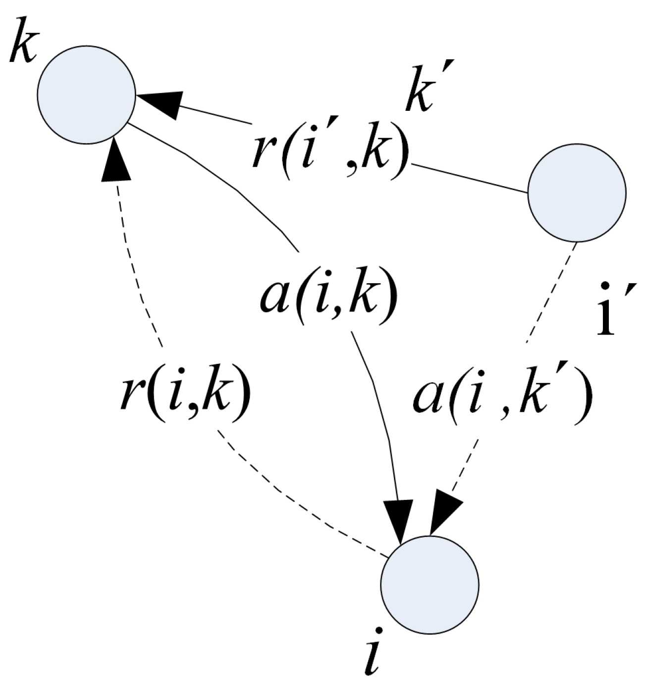
3.2. Affine Propagation Clustering Algorithm (AP)

The AP algorithm [46] is a clustering algorithm that was first proposed by Frey in 2007. Different from the K-means algorithm, the AP algorithm does not need to determine the number of clusters before running the algorithm. At the beginning of its operation, all sample points to be clustered can be regarded as potential clustering centers. Such potential clustering centers are called exemplars. The process of the AP algorithm to find cluster center is carried out according to the similarity between samples. The similarity matrix S is established by calculating the similarity between each sample point and other sample points. Assuming that the sample space is $\left\{x_1,x_2,\cdots ,x_n\right\}$ and $S\left(i,k\right)$ is the similarity between sample point $x_i$ and sample point $x_k$, $S\left(i,k\right)$ represents the similarity degree to which point $x_k$ can become the clustering center of point $x_i$.

$$S\left(i,k\right)=-{∥x_i-x_k∥}^2$$

(11)

The core of the AP algorithm is that there are two kinds of messages describing the sample situation between sample points, which are constantly updated iteratively. These two kinds of messages are attraction $r\left(i,k\right)$ and belonging $a\left(i,k\right)$. Figure 1 illustrates the exchange of these two messages.

Figure 1. AP algorithm indicates the transmission process of two kinds of messages.

In Figure 1, the dashed line represents the process of sending attractiveness, and the solid line represents the process of sending belongingness. The same point can be regarded as node i that supports node k as the cluster center in the process of attractiveness transmission, and it can also be regarded as node $k^{\prime }$ of the competitive candidate cluster center in the process of belongingness transmission. Attractiveness $r\left(i,k\right)$ describes the degree to which sample object k is suitable to serve as the clustering center of sample object i, and it represents the message sent by node i to k, which is updated by the attribution degree $a\left(i,k\right)$ and the similarity matrix S. The update rule is shown in Equation (12):

$$r(i,k)\leftarrow s(i,k)-max\{a(i,k^{\prime })+s(i,k^{\prime })\}(k^{\prime }\ne k)$$

(12)

where $s\left(i,k^{\prime }\right)$ represents the suitability of node $k^{\prime }$ as the clustering center of node i, and $a\left(i,k^{\prime }\right)$ represents the degree of recognition of node $k^{\prime }$ by node i. If $i=k$, then we have the following:

$$r(k,k)\leftarrow s(i,k)-max\left\{s(i,k^{\prime })\right\}(k^{\prime }\ne k)$$

(13)

Ascribing degree $a\left(i,k^{\prime }\right)$ describes the degree of recognition that sample object i selects sample object k as its clustering center, and it represents the message from k to i, which is updated by attraction $r\left(i,k^{\prime }\right)$, and its updating rule is shown in Equation (14):

$$a(i,k)\leftarrow min\{0,r(k,k)+\sum _{i^{\prime }.s.t.k^{\prime }\notin \{i,k\}}max\{0,r(i^{\prime },k)\}\}$$

(14)

If $i=k$, the self-attribution update rule is

$$\mathrm{a}(k,k)\leftarrow \sum _{i^{\prime }.s.t.k^{\prime }\notin \{i,k\}}max\{0,r(i^{\prime },k)\}$$

(15)

The algorithm transmits two messages alternately between the sample points, and the clustering centers remain unchanged after several iterations; finally, these high-quality clustering centers can be obtained.

3.3. Band Selection Based on Multi-Feature and Affine Propagation Clustering Algorithm

In traditional hyperspectral band selection methods based on clustering, single-information metrics such as mutual information, absolute distance, Euclidean distance, or divergence are used to construct similarity measures for band clustering. These methods predominantly employ the K-means algorithm, whose clustering results are highly sensitive to parameter settings. Therefore, this chapter proposes a hyperspectral band selection method based on multi-feature extraction and the AP clustering algorithm, which is referred to as GE-AP.

3.3.1. Similarity Matrix Construction

The AP algorithm is a process of finding cluster centers based on similarity, so constructing the similarity matrix is a key step in AP clustering. To address the issue of constructing similarity using single information, this study combines band texture features and Euclidean distance to construct the similarity matrix. The specific process is as follows:

Four texture features—contrast, correlation, energy, and entropy—can reflect comprehensive information about image clarity, texture thickness, and local gray-level correlation, as well as the amount of contained information. Assuming that the hyperspectral image has l bands, the GLCM of each band image in four directions (0°, 45°, 90°, 135°) is obtained. In this study, four $8\times 8$ matrices are generated for each band. Then, according to Equations (3)–(10), texture feature parameters such as contrast, correlation, energy, and entropy from the GLCMs in the four different directions of each band image are calculated. Finally, a $16\times 1$ dimensional feature vector $g_i={(g_{i1},g_{i2},\dots ,g_{i16})}^T$ is obtained for each band image, where i ranges from 1 to l.

The Euclidean distance (ED) is a well-established metric in the analysis of hyperspectral images, which are inherently represented as three-dimensional cubes. While texture features can effectively characterize the attributes of two-dimensional band images, it is essential to recognize that spectral relationship features also play a critical role in hyperspectral imagery. Therefore, we integrate band texture features with the Euclidean distance to construct a similarity matrix that encapsulates both the spectral characteristics of individual band images and the spatial information inherent in hyperspectral image data. The formula is as follows:

$$s(i,j)=-\sqrt{\sum _{x=1}^{16}{(g_{ix}-g_{ix})}^2}$$

(16)

where $g_i$ and $g_j$ represent the texture feature vectors of the I-band image and the J-band image. By calculating Equation (17), the similarity matrix S of hyperspectral images can be constructed, the size of which is $l\times l$, and expressed as follows:

$$S=\left[\begin{array}{c}-1S(1,2)\cdots S(1,j)\cdots S(1,l)\hfill \\ S(2,1)-1\cdots S(2,j)\cdots S(2,l)\hfill \\ ⋮⋮⋮⋮\hfill \\ S(i,1)S(i,2)\cdots S(i,j)\cdots S(i,l)\hfill \\ ⋮⋮⋮⋮\hfill \\ S(l,1)S(l,2)\cdots S(l,j)\cdots -1\hfill \end{array}\right],i\in [1,l]j\in [1,l]$$

(17)

3.3.2. Band Selection Process of Affine Propagation Clustering Algorithm

The AP clustering algorithm is employed to cluster images in hyperspectral bands. This method overcomes the challenges of selecting the k value in K-means clustering and the issue that the initial cluster centers significantly influence the clustering results. In the AP algorithm, each band is initially considered as a potential cluster center. Subsequently, based on the proposed band similarity matrix, the algorithm calculates the attraction and belongingness between the updated bands, ultimately completing the clustering process. The clustering results obtained using this method are more stable and efficient.

3.3.3. Band Selection Framework Based on GE-AP Algorithm

Based on the aforementioned ideas, this paper proposes a band selection method for hyperspectral images using multi-feature extraction and AP clustering. Firstly, texture features of the band images are extracted, and then the Euclidean distance is used to describe the spectral relationships between band images. The similarity matrix is constructed by combining texture features and the Euclidean distance. Subsequently, the AP clustering algorithm continuously updates the attraction and belonging degree of bands based on the similarity matrix, ultimately yielding several high-quality and stable cluster center bands. These cluster center bands serve as representative bands to achieve dimensionality reduction, thereby facilitating subsequent classification processing and other applications. The specific workflow of this algorithm for hyperspectral image band selection is illustrated in Figure 2.

Figure 2. Band selection flow chart based on multi-feature and Affine Propagation Clustering algorithm.

4. Experiment

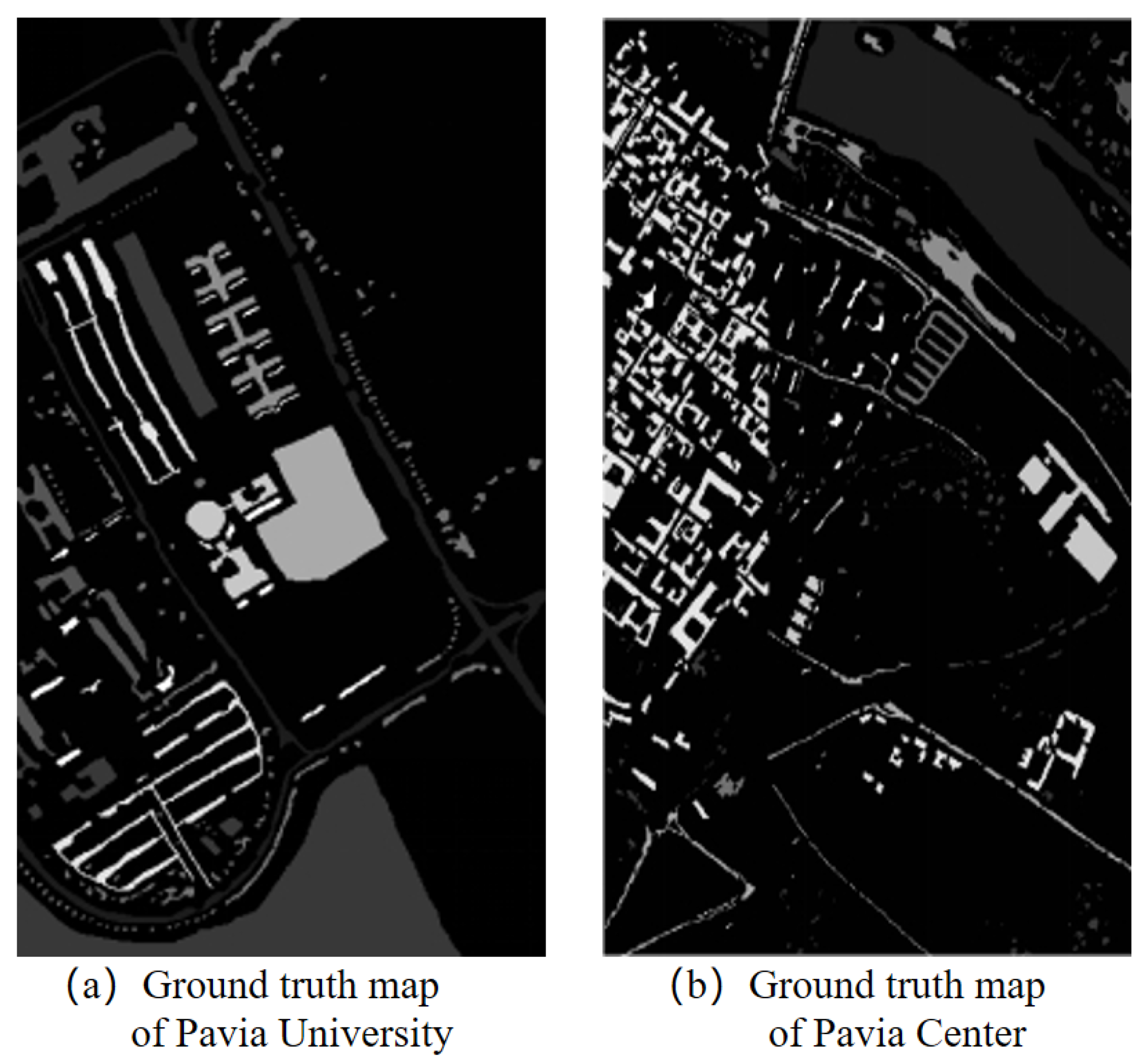
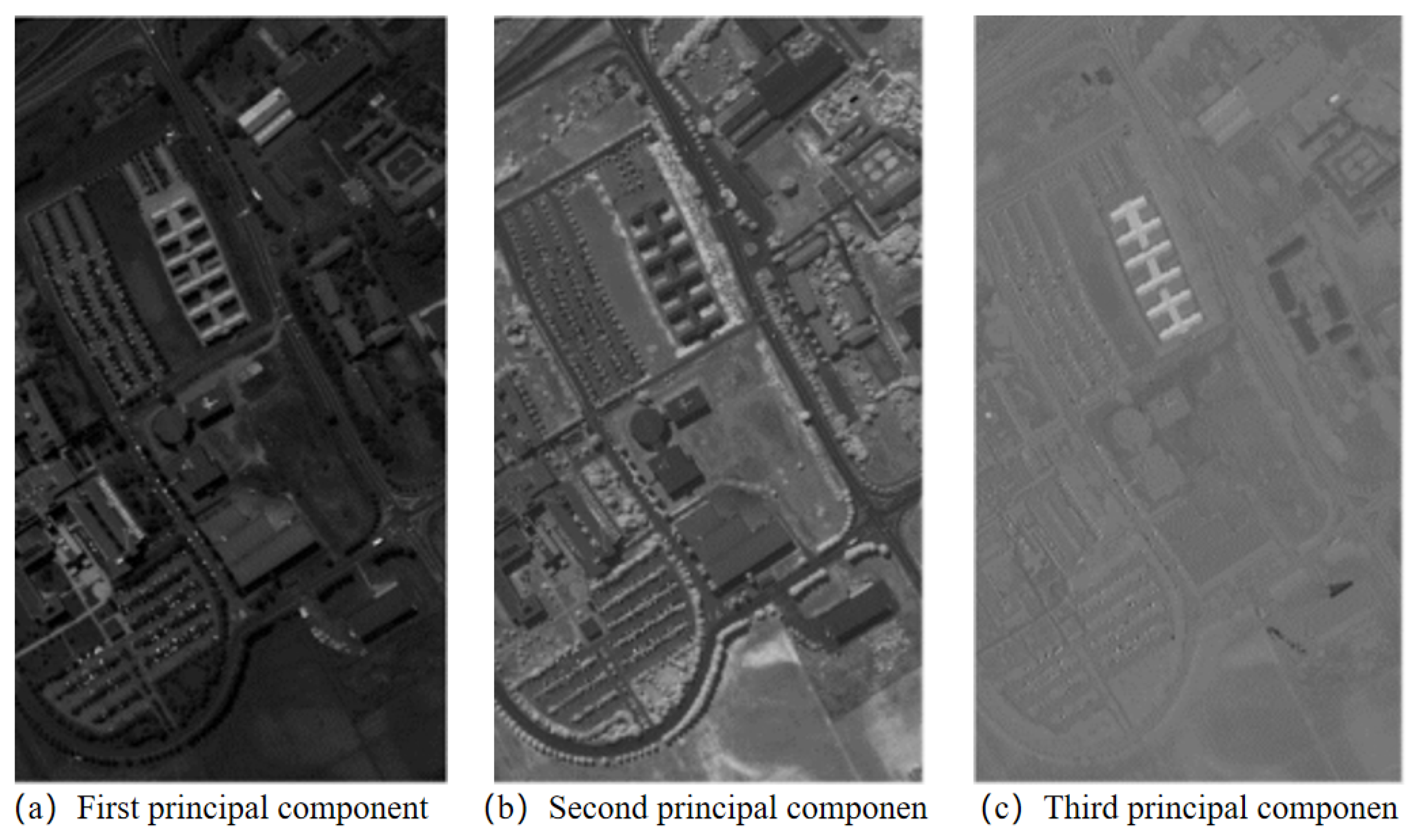
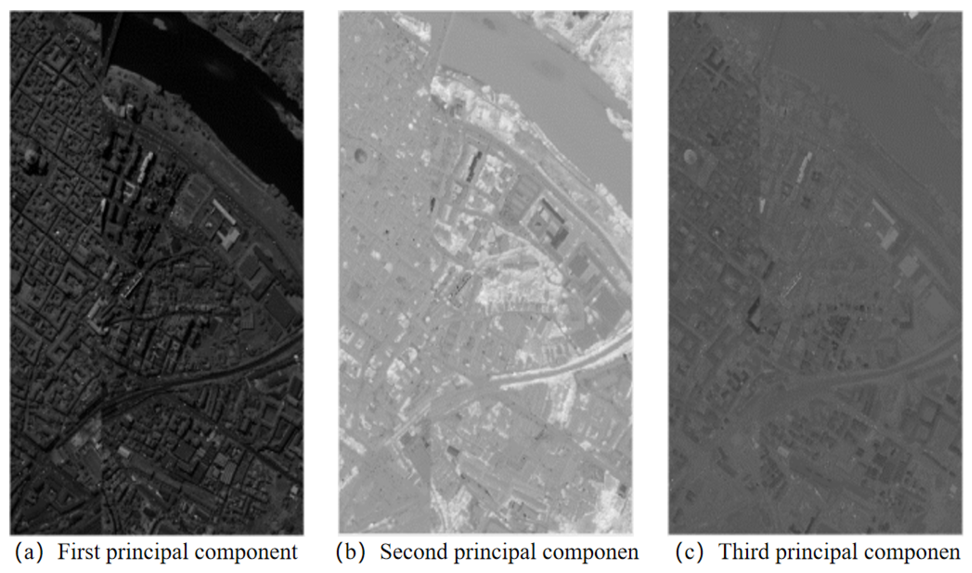
4.1. Experimental Setup

All algorithms were executed on an Intel Core i7 4.2GHz processor with 16 GB RAM, without any acceleration methods. This section introduces the hyperspectral image datasets used in the subsequent simulation experiments, namely, the internationally recognized Pavia University and Pavia Center scenes [47].

For the Pavia University scene, the image dimensions for each spectral band are provided. The original image contains 115 spectral bands. However, due to noise interference affecting 12 of these bands, only 103 bands were utilized in the experimental simulations. The dataset includes nine categories of ground objects: Asphalt, Meadows, Gravel, Trees, Metal Sheets, Bare Soil, Bitumen, Bricks, and Shadows. Figure 3a presents the ground truth map of the Pavia University hyperspectral image.

Figure 3. Real object distribution map.

The Pavia Center scene contains 115 spectral bands, but 13 of these bands are affected by noise, leaving 102 bands for the experimental simulations. The dataset includes nine categories of ground objects: Water, Trees, Asphalt, Bricks, Bitumen, Tiles, Shadows, Meadows, and Bare Soil. Figure 3b shows the ground truth map of the Pavia Center hyperspectral image.

4.2. Compare the Experimental Simulation Results

To verify the effectiveness of the hyperspectral image band selection method based on multi-feature extraction and AP clustering, this study compares it with three other methods: feature extraction based on maximized variance PCA (MVPCA) [48], band selection based on ABS, band selection based on ASP, Genetic algorithms (GAs) [49] and spectral–spatial GA-based unsupervised Band selection (SSGA) [50]. The following section describes the simulation process and results for feature extraction applied to hyperspectral images of Pavia University and Pavia Center using these comparison methods.

In the theory of maximum variance, it is assumed that after reducing the dimensionality of a sample to k dimensions, the variance on each dimension represents the optimal k-dimensional representation. By combining the maximum variance theory with PCA, we can extract the most informative features. This method is referred to as MVPCA. In MVPCA, all bands of hyperspectral images are linearly transformed. After transformation, the information in the hyperspectral images is concentrated primarily in the first few uncorrelated principal components, which can be inversely transformed to approximate the original image. Therefore, when used, the first several principal components are typically selected.

In general, the Principal Component Analysis method reduces dimensionality by selecting principal components whose eigenvalues are greater than 1. Table 1 shows the percentage of the sum of squares extracted by principal components with eigenvalues greater than 1 from the hyperspectral images of Pavia University after Principal Component Analysis.

Table 1. Percentage of sum of squares extracted from hyperspectral images by Pavia University.

Ingredient	Extract the Percentage of the Sum of Squares
	Eigenvalue	Percentage Contribution of Variance%	Cumulative Percentage%
1	66.792	64.847	64.847
2	29.310	28.456	93.303
3	5.289	5.135	98.439

As shown in Table 1, after the transformation of hyperspectral images of Pavia University, there were three principal components with eigenvalues greater than 1. Their eigenvalues are 66.792, 29.310, and 5.289. The contribution rates of these three principal components came out to 64.847%, 28.456%, and 5.135%, respectively, with a cumulative contribution rate of 98.439%. The feature map obtained after inverse transformation is illustrated in Figure 4.

Figure 4. Pavia University hyperspectral image of the first three principal component images.

Figure 5a shows the scree plot of each principal component and its corresponding eigenvalue after the transformation of the hyperspectral images of Pavia University. As can be seen from the figure, the slopes of the first three principal components are relatively steep, while the slopes of components 4 to 103 are nearly flat, approaching zero. In conjunction with the contribution rates listed in Table 1, it is evident that the first three principal components capture the majority of the variance. Therefore, for the hyperspectral images of Pavia University, the first three principal components were selected.

Figure 5. Hyperspectral image component lithotripsy.

Table 2 shows the percentage of the sum of squares extracted from the principal components of Pavia Center hyperspectral images whose eigenvalue is greater than 1 after Principal Component Analysis.

Table 2. Percentage of sum of squares extracted from hyperspectral images by Pavia Center.

Ingredient	Extract the Percentage of the Sum of Squares
	Eigenvalue	Percentage Contribution of Variance%	Cumulative Percentage%
1	74.307	72.850	72.850
2	21.447	21.026	93.876
3	4.316	4.232	98.108

As shown in Table 2, after the transformation of hyperspectral images of the Pavia Center, there were three principal components with eigenvalues greater than 1. Their eigenvalues are 74.307, 21.447, and 4.316. The contribution rates of these three principal components are 72.850%, 21.026%, and 4.232%, respectively, with a cumulative contribution rate of 98.108%. The feature map obtained after inverse transformation is illustrated in Figure 6.

Figure 6. Pavia Center hyperspectral image of the first three principal component images.

Figure 5b shows the scree plot of each principal component and its corresponding eigenvalue after the transformation of hyperspectral images of the Pavia Center. As can be seen from the figure, the first three components exhibit steeper slopes and larger eigenvalues, while the slopes of subsequent components are nearly flat, approaching zero. Therefore, based on this analysis, the first three principal components were selected for the hyperspectral images of the Pavia Center.

As shown in the figure, the first three components have steep slopes with large eigenvalues, while the slopes of the remaining components approach zero, forming a gentle tail. In conjunction with the contribution rates listed in Table 2, it is evident that the first three principal components captured the majority of the variance. Therefore, the first three principal components of the hyperspectral images of the Pavia Center were selected through analysis. Consequently, both the hyperspectral images of Pavia University and Pavia Center utilized Principal Component Analysis to project from high-dimensional space to low-dimensional space. Specifically, the 103 bands of the Pavia University hyperspectral images were reduced to three principal components, and the 102 bands of Pavia Center hyperspectral images were similarly transformed into three principal components.

Figure 7a illustrates the band index line chart for the 103 bands of hyperspectral images of Pavia University using the adaptive band selection method. Since the GE-AP method selects 10 bands for hyperspectral images of Pavia University, the first 10 bands selected by the ABS method were used for experimental comparison. The serial numbers of the first 10 bands with the highest band index values are 91, 88, 90, 89, 87, 92, 93, 95, 94, and 96. Table 3 lists the band index values corresponding to these 10 selected bands for Pavia University and the 11 selected bands for the Pavia Center hyperspectral images.

Figure 7. Band index line plots of hyperspectral images of Pavia University and Pavia Cener based on ABS method.

Table 3. Band index of hyperspectral images of Pavia University and Pavia Center based on ABS method.

Pavia University		Pavia Center
Band Number	Band Index	Band Number	Band Index
91	872.9048	91	1114.185
88	871.5208	90	1111.205
90	870.9870	88	1110.937
89	870.7075	89	1110.31
87	870.1934	92	1109.339
92	869.1692	87	1107.67
93	863.9795	93	1102.059
95	863.7521	95	1101.782
94	863.5711	94	1101.5
96	857.7908	82	1095.023
		96	1094.566

Figure 7b shows the band index line chart for the 102 bands of hyperspectral images of the Pavia Center using the adaptive band selection method. As the GE-AP method proposed in this section selected 11 bands for hyperspectral images of Pavia Center, the first 11 bands selected by the ABS method were used for experimental comparison. The serial numbers of the first 11 bands with the highest band index values are 91, 90, 88, 89, 92, 87, 93, 95, 94, 82, and 96.

The automatic subspace partitioning (ASP) method is a band selection technique that leverages the blocking characteristics of the correlation coefficient matrix of hyperspectral images. The gray-scale image of the band correlation coefficient matrix exhibits distinct blocking features, which allows for the division of independent subspaces within hyperspectral images. Subsequently, bands are selected from these segmented subspaces, taking into account both band correlation and information content.

Figure 8a represents a Pavia University image, and Figure 8b represents a Pavia Center image. Both images clearly exhibit blocked structures in their correlation coefficient matrices. After obtaining the correlation matrix of the hyperspectral image, the nearest transitive vector could be derived, and the local minimum points of this vector could be extracted to identify the nodes for subspace partitioning.

Figure 8. Grayscale of correlation coefficient.

Figure 9a illustrates the near-neighbor transitive correlation curve for hyperspectral images from the Pavia University. It is evident that there are two local minima in the near-neighbor transitive vectors, indicating that the image could be divided into three independent subspaces. The band serial numbers for each subspace are as follows: bands 61 to 64, bands 82 to 84, and bands 101 to 103.

Figure 9. The nearest neighbors of hyperspectral images can transmit correlation curves.

Figure 10a–c shows the line diagrams of band coefficients in each corresponding subspace. The band coefficients in the three subspaces were calculated separately. Finally, 10 bands were selected for comparison experiments based on the band coefficients in each subspace, with the band serial numbers being 63, 62, 61, 64, 84, 83, 82, 103, 102, and 101.

Figure 10. Line chart of band coefficients in each subspace of hyperspectral image.

Figure 9b illustrates the near-neighbor transitive correlation curve for hyperspectral images from Pavia Center. Similarly, there were two local minima in the near-neighbor transitive vectors, indicating that the image could be divided into three independent subspaces. The band serial numbers for each subspace are as follows: bands 63 to 65, bands 73 to 84, and bands 99 to 102.

Figure 10d–f shows the line diagrams of the band coefficients in each subspace of hyperspectral images of the Pavia Center. The band coefficients in the three subspaces were calculated separately. Finally, 11 bands were selected for comparison experiments based on the band coefficients in each subspace, with the band serial numbers being 64, 63, 73, 65, 84, 83, 82, 102, 101, 100, and 99.

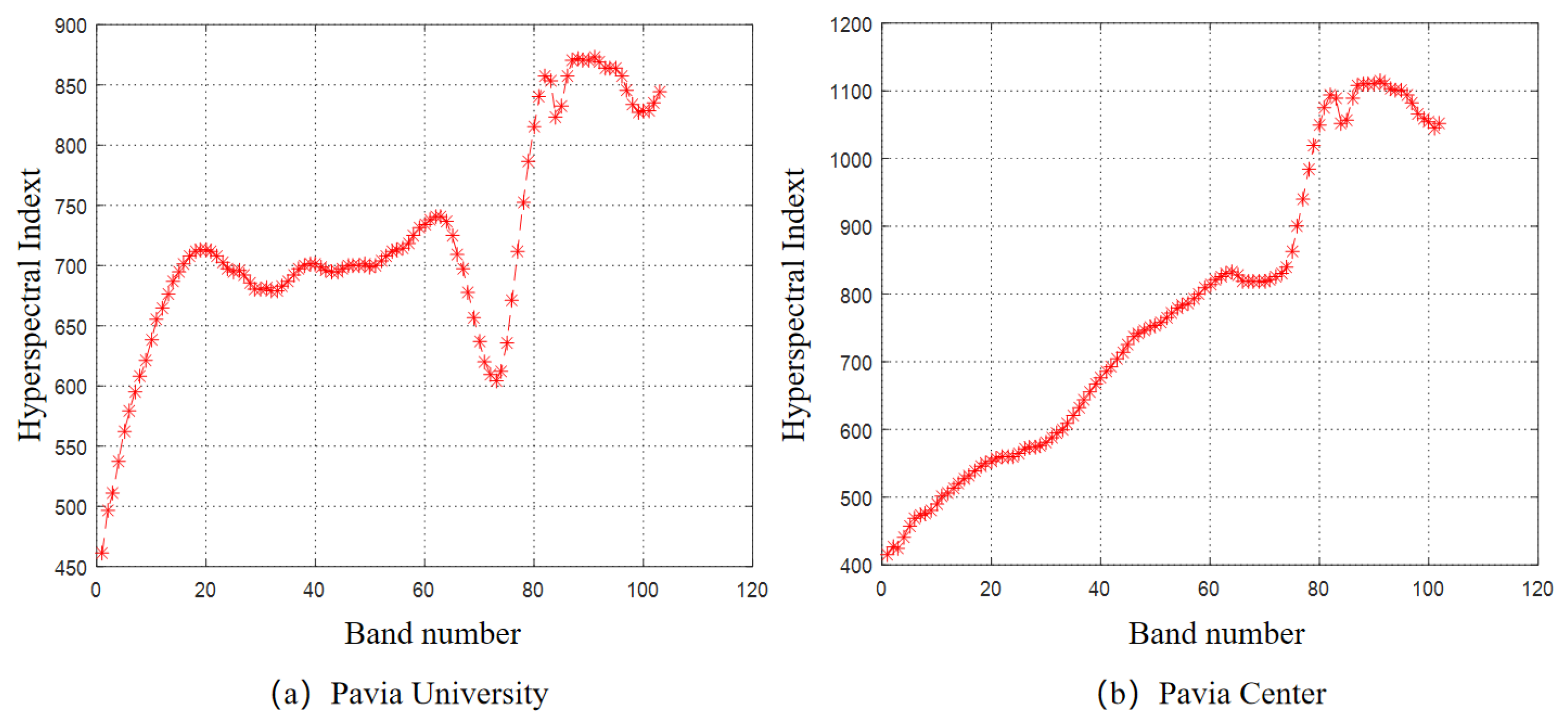
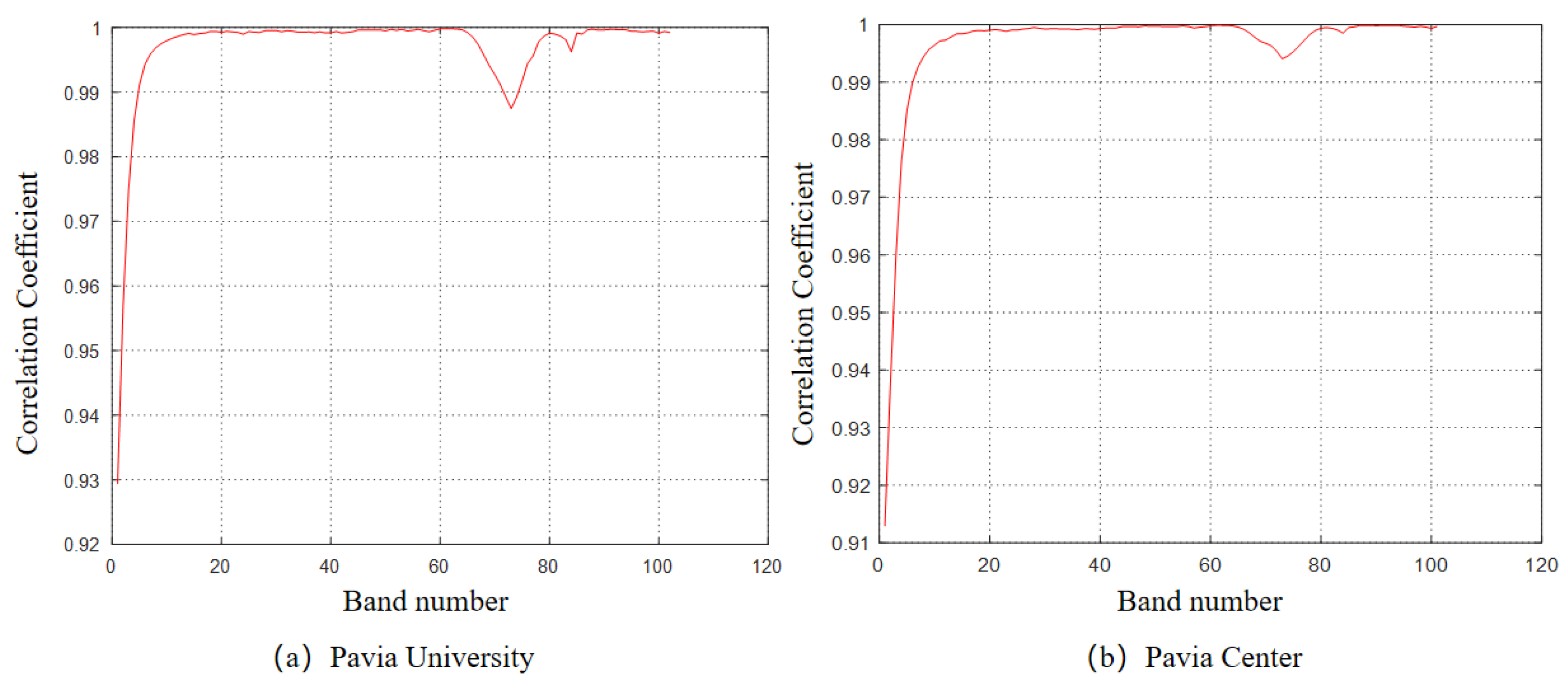
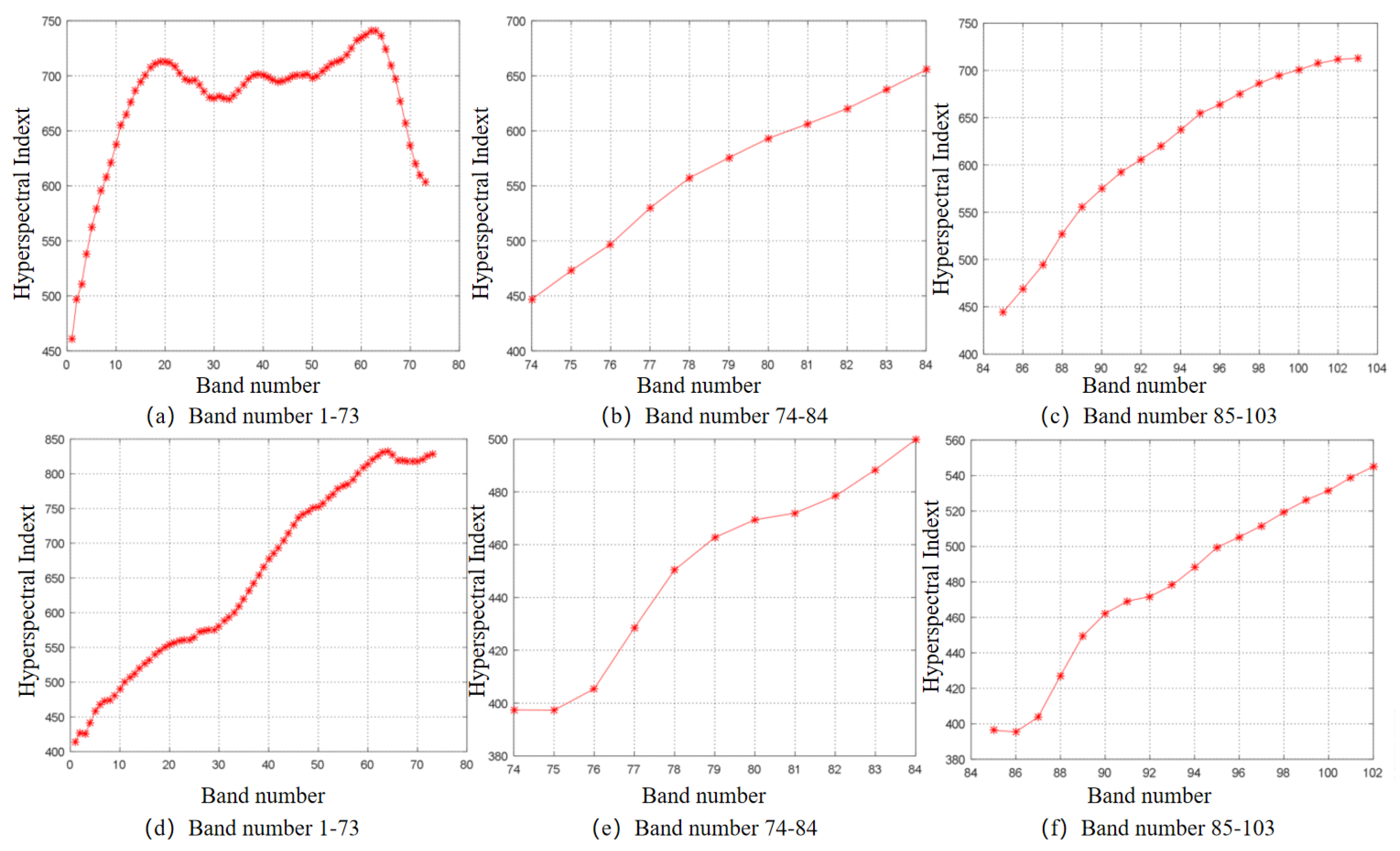
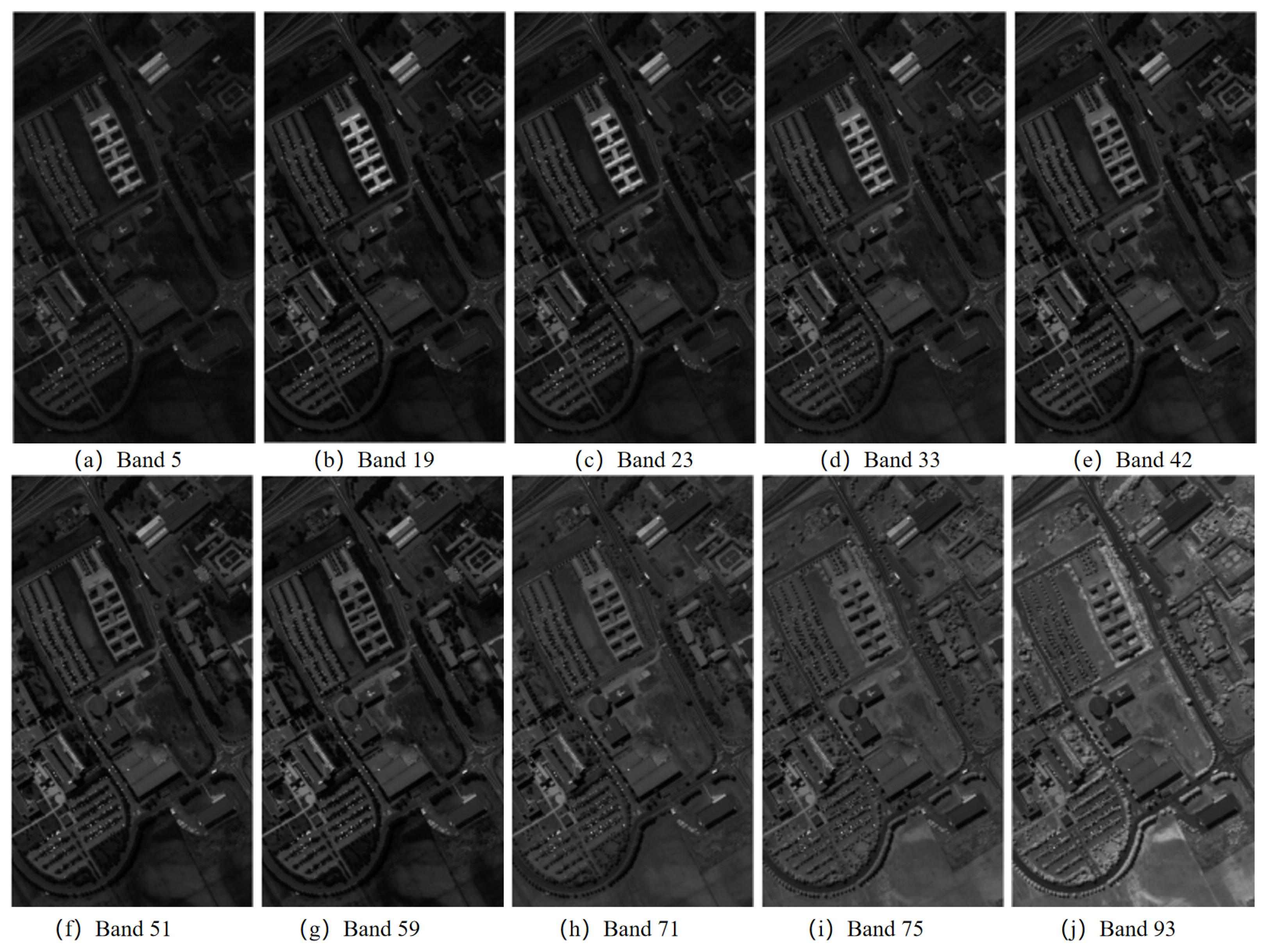
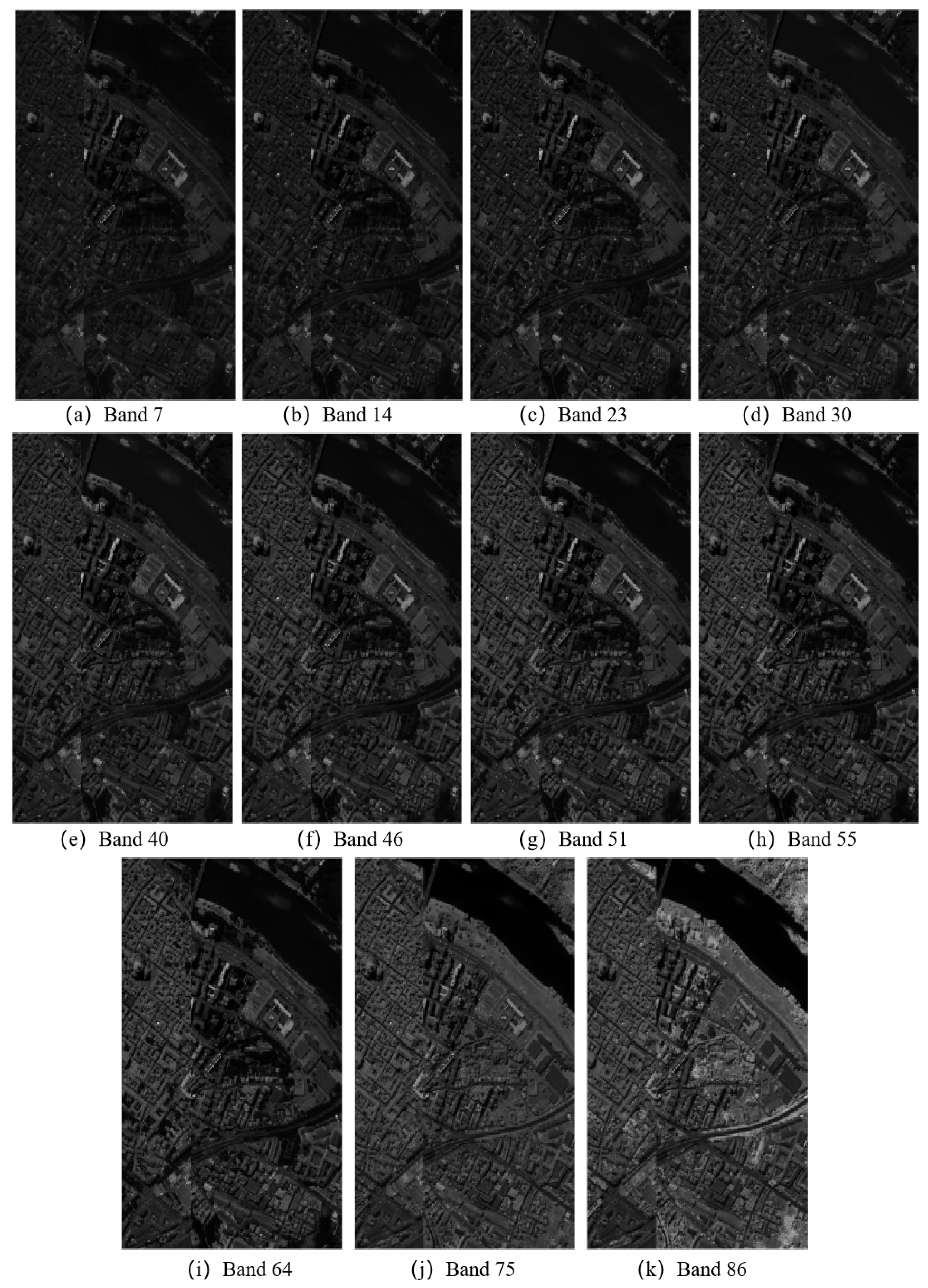
4.3. Experimental Results of Band Selection Based on GE-AP Algorithm

According to the principle of the GE-AP algorithm, the texture features of hyperspectral band images were first extracted. Subsequently, a similarity matrix was constructed by combining Euclidean distance. Finally, the AP algorithm was employed to cluster all the band images. Table 4 presents the clustering results and the cluster center bands for the hyperspectral images of Pavia University after applying the GE-AP method. It can be seen that the 103 bands of the hyperspectral image of Pavia University were classified into 10 categories, thereby selecting 10 representative bands from the original 103 bands for subsequent processing and achieving dimensionality reduction. The cluster centers listed in Table 4 represent the selected bands, with their respective band numbers being 5, 19, 23, 33, 42, 51, 59, 71, 85, and 93. Representative images of each selected band are shown in Figure 11.

Table 4. Pavia University image clustering results.

Cluster Center Band Number	Number of Bands per Class	Band Number of Each Class
5	7	3~9
19	9	13~21
23	7	10~12, 22~25
33	15	26~37, 67~69
42	10	38~46, 66
51	11	47~56, 65
59	8	57~64
71	5	2, 70~73
75	5	1, 74~77
93	26	78~103

Figure 11. The Pavia University band represents the image.

Table 5 presents the clustering results and central bands of the hyperspectral images of Pavia Center after applying the GE-AP method. It can be seen that the 102 bands of the hyperspectral image of Pavia Center were classified into 11 categories, thereby selecting 11 representative bands from the original 102 bands for subsequent processing and achieving dimensionality reduction. The cluster centers listed in Table 5 represent the selected bands, with their respective band numbers being 7, 14, 23, 30, 40, 46, 51, 55, 64, 75, and 86. Representative images of each selected band are shown in Figure 12.

Table 5. Pavia Center image clustering results.

Cluster Center Band Number	Number of Bands per Class	Band Number of Each Class
7	10	3~12
14	9	13~21
23	4	2, 22, 23, 24
30	12	1, 25~35
40	9	36~44
46	3	45, 46, 47
51	9	48~53, 68, 69, 70
55	5	54~56, 66, 67
64	9	57~65
75	8	71~78
86	24	79~102

Figure 12. The Pavia Center band represents the image.

By combining the multi-feature and Affine Propagation Clustering algorithm, the band selection of two hyperspectral images was carried out to achieve a significant reduction in the number of bands. The representative bands selected by the method in this section were classified and compared with the bands selected by the three methods introduced in the previous section. In each hyperspectral image in the classification experiment, 10% of each type of ground object was randomly selected as the training sample, and the remaining 90% was used as the test sample.

Table 6 presents the classification results of hyperspectral images from the Pavia University scenes following feature extraction conducted through six distinct methods: MVPCA, ABS, ASP, GA, SSGA, and GE-AP. The overall OA and Kappa coefficient metrics were used to evaluate the performance of these methods. As shown in the table, the GE-AP method achieved the highest classification accuracy at 88.21%, representing a maximum increase of 7.34% compared to other methods. Additionally, the Kappa coefficient for the GE-AP method was the highest at 0.838, indicating a maximum improvement of 9.97% over other methods. The Pavia Center hyperspectral images after feature extraction using MVPCA, ABS, ASP, GA, SSGA, and GE-AP are shown. As shown in the table, the OA of the GE-AP method was the highest among the four methods, reaching 98.63%, which represents a maximum increase of 8.89% compared to the other methods. Additionally, the Kappa coefficient for the GE-AP method reached 0.979, indicating a maximum improvement of 13.18% over the other methods.

Table 6. Hyperspectral image classification results from Pavia University and Pavia Center. The top two scores are represented in red and blue, respectively.

Dataset	Methods	OA%	Kappa
	MVPCA	82.18	0.762
	ABS	85.95	0.811
Pavia	ASP	87.95	0.836
University	GA	84.12	0.784
	SSGA	88.45	0.846
	GE-AP	88.21	0.838
	MVPCA	97.65	0.967
	ABS	90.58	0.865
Pavia	ASP	97.12	0.959
Center	GA	84.12	0.784
	SSGA	97.28	0.962
	GE-AP	98.63	0.979

The image size of the Pavia Center images is 1096 × 1096, and that of Pavia University is 610 × 610. As a heuristic search algorithm, SSGA can efficiently obtain the global optimal solution in smaller remote sensing images, but it faces challenges in achieving the global optimal solution when the search space is large. From the experimental results of the two hyperspectral images, it can be seen that the band selection method based on GE-AP proposed in this paper can effectively select representative band subsets, and it is more in line with the current trend of increasing resolution of remote sensing images.

5. Conclusions

To address the challenge of band selection based on clustering, this paper proposed a band selection method for hyperspectral images that integrates multi-feature extraction and the AP clustering algorithm. Firstly, the texture features of the band images were extracted using the GLCM, which captures the two-dimensional spatial characteristics of hyperspectral data. Next, the Euclidean distance between bands was calculated based on these texture features, reflecting the spectral relationships within the hyperspectral image while being insensitive to variations in spectral amplitude. Subsequently, a similarity matrix was constructed based on the comprehensive features of the bands. The AP clustering algorithm was then applied to cluster the bands according to the similarity matrix, with the cluster centers selected as representative bands. Finally, the results demonstrate that this method achieved a maximum increase of 8.89% in overall classification accuracy OA and 13.18% in its Kappa coefficient value, thereby highlighting its superiority.

References

1. Cozzolino, D.; Williams, P.; Hoffman, L. An overview of pre-processing methods available for hyperspectral imaging applications. Microchem. J. 2023, 193, 109129. [Google Scholar] [CrossRef]
2. Cheng, X.; Huo, Y.; Lin, S.; Dong, Y.; Zhao, S.; Zhang, M.; Wang, H. Deep feature aggregation network for hyperspectral anomaly detection. IEEE Trans. Instrum. Meas. 2024, 73, 5033016. [Google Scholar] [CrossRef]
3. Shaik, R.U.; Periasamy, S.; Zeng, W. Potential assessment of PRISMA hyperspectral imagery for remote sensing applications. Remote. Sens. 2023, 15, 1378. [Google Scholar] [CrossRef]
4. Khan, A.; Vibhute, A.D.; Mali, S.; Patil, C. A systematic review on hyperspectral imaging technology with a machine and deep learning methodology for agricultural applications. Ecol. Inform. 2022, 69, 101678. [Google Scholar] [CrossRef]
5. Vivone, G. Multispectral and hyperspectral image fusion in remote sensing: A survey. Inf. Fusion 2023, 89, 405–417. [Google Scholar] [CrossRef]
6. Cheng, X.; Zhang, M.; Lin, S.; Zhou, K.; Zhao, S.; Wang, H. Two-stream isolation forest based on deep features for hyperspectral anomaly detection. IEEE Geosci. Remote. Sens. Lett. 2023, 20, 5504205. [Google Scholar] [CrossRef]
7. Huo, Y.; Cheng, X.; Lin, S.; Zhang, M.; Wang, H. Memory-augmented Autoencoder with Adaptive Reconstruction and Sample Attribution Mining for Hyperspectral Anomaly Detection. IEEE Trans. Geosci. Remote. Sens. 2024, 62, 5518118. [Google Scholar] [CrossRef]
8. Mou, L.; Saha, S.; Hua, Y.; Bovolo, F.; Bruzzone, L.; Zhu, X.X. Deep reinforcement learning for band selection in hyperspectral image classification. IEEE Trans. Geosci. Remote. Sens. 2021, 60, 5504414. [Google Scholar] [CrossRef]
9. Fu, B.; Sun, X.; Cui, C.; Zhang, J.; Shang, X. Structure-preserved and weakly redundant band selection for hyperspectral imagery. IEEE J. Sel. Top. Appl. Earth Obs. Remote. Sens. 2024, 17, 12490–12504. [Google Scholar] [CrossRef]
10. Zhuang, J.; Zheng, Y.; Guo, B.; Yan, Y. Globally Deformable Information Selection Transformer for Underwater Image Enhancement. IEEE Trans. Circuits Syst. Video Technol. 2024. [Google Scholar] [CrossRef]
11. Lever, J.; Krzywinski, M.; Altman, N. Principal Component Analysis. Nat. Methods 2017, 14, 641–642. [Google Scholar] [CrossRef]
12. Li, Y.; Zhang, M.; Bian, X.; Tian, L.; Tang, C. Progress of Independent Component Analysis and Its Recent Application in Spectroscopy Quantitative Analysis. Microchem. J. 2024, 202, 110836. [Google Scholar] [CrossRef]
13. Zhao, S.; Zhang, B.; Yang, J.; Zhou, J.; Xu, Y. Linear Discriminant Analysis. Nat. Rev. Methods Prim. 2024, 4, 70. [Google Scholar] [CrossRef]
14. Dash, S.; Chakravarty, S.; Giri, N.C.; Agyekum, E.B.; AboRas, K.M. Minimum Noise Fraction and Long Short-Term Memory Model for Hyperspectral Imaging. Int. J. Comput. Intell. Syst. 2024, 17, 16. [Google Scholar] [CrossRef]
15. Chavez, P.S.; Kwarteng, A.Y. Extracting spectral contrast in Landsat thematic mapper image data using selective principal component analysis. Photogramm. Eng. Remote. Sens. 1989, 57, 339–348. [Google Scholar]
16. Jia, X.P.; Richards, J.A. Segmented principal components transformation for efficient hyperspectral remote image display and classification. IEEE Trans. Geosci. Remote. Sens. 1999, 37, 538–542. [Google Scholar]
17. Mika, S.; Ratsch, G.; Weston, J.; Scholkopf, B.; Mullers, K.R. Fisher discriminant analysis with kernels. In Proceedings of the Neural Networks for Signal Processing IX, Madison, WI, USA, 25 August 1999. [Google Scholar]
18. Velasco-Forero, S.; Angulo, J.; Chanussot, J. Morphological image distances for hyperspectral dimensionality exploration using Kernel-PCA and ISOMAP. In Proceedings of the Geoscience and Remote Sensing Symposium, Cape Town, South Africa, 12–17 July 2009; pp. III-109–III-112. [Google Scholar]
19. He, X.F.; Niyogi, P. Locality preserving projections. In Proceedings of the Annual Conference on Neural Information Processing Systems, New Orleans, LA, USA, 10–16 December 2023; pp. 153–160. [Google Scholar]
20. Ma, L.; Crawford, M.M.; Tian, J. Local manifold learning-based k-nearest neighbor for hyperspectral image classification. IEEE Trans. Geosci. Remote. Sens. 2010, 48, 4099–4109. [Google Scholar] [CrossRef]
21. Liu, C.; Zhao, C.; Zhang, L. A New Dimensionality Reduction Method for Hyperspectral Images. J. Image Graph. 2005, 10, 218–222. [Google Scholar]
22. Tang, W.; Hu, J.; Zhang, H.; Wu, P.; He, H. Kappa Coefficient: A Popular Measure of Rater Agreement. Shanghai Arch. Psychiatry 2015, 27, 62–67. [Google Scholar]
23. Zhang, B.; Wang, X.; Liu, J.; Zheng, L.; Tong, Q. Hyperspectral image processing and analysis system (HIPAS) and its applications. Photogramm. Eng. Remote. Sens. 2000, 66, 605–609. [Google Scholar]
24. Chavez, P.S.; Berlin, G.L.; Sowers, L.B. Statistical method for selecting Landsat MSS ratio. J. Appl. Photogr. Eng. 1982, 1, 23–30. [Google Scholar]
25. Charles, S. Selecting band combination from multispectral data. Photogramm. Eng. Remote. Sens. 1985, 51, 681–687. [Google Scholar]
26. Velez-Reyes, M.; Linares, D.M. Comparison of principal-component-based band selection methods for hyperspectral imagery. In Proceedings of the International Symposium on Remote Sensing, Toulouse, France, 17–21 September 2021; SPIE: St Bellingham, WA, USA, 2002; pp. 361–369. [Google Scholar]
27. Nakariyakul, S.; Casasent, D.P. Hyperspectral waveband selection for contaminant detection on poultry carcasses. Opt. Eng. 2008, 47, 1–9. [Google Scholar]
28. Diani, M.; Acito, N.; Greco, M.; Corsini, G. A new band selection strategy for target detection in hyperspectral images. Knowl.-Based Intell. Inf. Eng. Syst. 2008, 5159, 424–431. [Google Scholar]
29. Omam, M.A.; Torkamani-Azar, F. Band selection of hyperspectral-image based on weighted independent component analysis. Opt. Rev. 2010, 17, 367–370. [Google Scholar] [CrossRef]
30. Fisher, K.; Chang, C.I. Progressive band selection for satellite hyperspectral data compression and transmission. J. Appl. Remote. Sens. 2010, 4, 041770. [Google Scholar]
31. Gu, Y.; Zhang, Y. Feature extraction of hyperspectral data based on automatic subspace division. Remote. Sens. Technol. Appl. 2003, 18, 801–804. [Google Scholar]
32. Ni, G.; Shen, Y. Wavelet-Based Principal Components Analysis Feature Extraction Method for Hyperspectral Images. Trans. Beijing Inst. Technol. 2007, 7, 621–624. [Google Scholar]
33. Luo, R.; Pi, Y. Supervised Neighborhood Preserving Embedding Feature Extraction of Hyperspectral Imagery. Acta Geod. Cartogr. Sin. 2014, 43, 508–513. [Google Scholar]
34. Ding, L.; Tang, P.; Li, H. Mixed spectral unmixing analysis based on manifold learning. Infrared Laser Eng. 2013, 9, 2421–2425. [Google Scholar]
35. Qian, Y.; Yao, F.; Jia, S. Band selection for hyperspectral imagery using affinity propagation. IET Comput. Vis. 2009, 3, 213–222. [Google Scholar] [CrossRef]
36. Yin, J.; Wang, Y.; Zhao, Z. Optimal band selection for hyperspectral image classification based on inter-class separability. In Proceedings of the 2010 Symposium on Photonics and Optoelectronics, Chengdu, China, 19–21 June 2010; pp. 1–4. [Google Scholar]
37. Jia, S.; Ji, Z.; Qian, Y.; Shen, L. Unsupervised band selection for hyperspectral imagery classification without manual band removal. IEEE J. Sel. Top. Appl. Earth Obs. Remote. Sens. 2012, 5, 531–543. [Google Scholar] [CrossRef]
38. Guo, Z.; Zhang, D.; Zhang, L. Feature band selection for online multispectral palmprint recognition. IEEE Trans. Inf. Forensics Secur. 2012, 7, 1094–1099. [Google Scholar] [CrossRef]
39. Zhao, H.; Li, M.; Li, N. A band selection method based on improved subspace partition. Infrared Laser Eng. 2015, 44, 3155–3160. [Google Scholar]
40. Guo, T.; Hua, W.; Liu, X. Rapid hyperspectral band selection approach based on clustering and optimal index algorithm. Opt. Tech. 2016, 42, 496–500. [Google Scholar]
41. Zhang, A.; Du, N.; Kang, X.; Guo, C. Hyperspectral adaptive band selection method through nonlinear transform and information adjacency correlation. Infrared Laser Eng. 2017, 46, 05308001. [Google Scholar]
42. Zhai, H.; Zhang, H.; Zhang, L. Spectral-spatial clustering of hyperspectral remote sensing image with sparse subspace clustering model. In Proceedings of the 2015 7th Workshop on Hyperspectral Image and Signal Processing: Evolution in Remote Sensing (WHISPERS), Tokyo, Japan, 2–5 June 2015; pp. 1–4. [Google Scholar]
43. Zhai, H.; Zhang, H.; Zhang, L. Squaring weighted low-rank subspace clustering for hyperspectral image band selection. In Proceedings of the 2016 IEEE International Geoscience and Remote Sensing Symposium (IGARSS), Beijing, China, 10–15 July 2016; pp. 2434–2437. [Google Scholar]
44. Haralick, R.M.; Shanmugarm, K.; Dinstein, I. Textural features for image classification. IEEE Trans. Syst. Man Cybern. 1973, 3, 610–621. [Google Scholar] [CrossRef]
45. Ulaby, F.T.; Kouyate, F.; Brisco, B.; Williams, T.L. Textural information in SAR Images. IEEE Trans. Geosci. Remote Sens. 1986, 24, 235–245. [Google Scholar] [CrossRef]
46. Frey, B.J.; Dueck, D. Clustering by passing messages between data points. Science 2007, 315, 972–976. [Google Scholar] [CrossRef]
47. Pavia University and Pavia Center Hyperspectral Datasets. Available online: http://www.ehu.eus/ccwintco/index.php/Hyperspectral_Remote_Sensing_Scenes#Pavia_Centre_and_University (accessed on 15 October 2024).
48. Chang, C.I.; Du, Q.; Sun, T.L.; Althouse, M.L. A joint band prioritization and band-decorrelation approach to band selection for hyperspectral image classification. IEEE Trans. Geosci. Remote. Sens. 1999, 37, 2631–2641. [Google Scholar] [CrossRef]
49. Huang, R.; Li, X. Band selection based on evolution algorithm and sequential search for hyperspectral classification. In Proceedings of the 2008 International Conference on Audio, Language and Image Processing, Shanghai, China, 7–9 July 2008; IEEE: Piscataway, NJ, USA, 2008; pp. 1270–1273. [Google Scholar]
50. Zhao, H.; Bruzzone, L.; Guan, R.; Zhou, F.; Yang, C. Spectral-spatial genetic algorithm-based unsupervised band selection for hyperspectral image classification. IEEE Trans. Geosci. Remote. Sens. 2021, 59, 9616–9632. [Google Scholar] [CrossRef]
Disclaimer/Publisher’s Note: The statements, opinions and data contained in all publications are solely those of the individual author(s) and contributor(s) and not of MDPI and/or the editor(s). MDPI and/or the editor(s) disclaim responsibility for any injury to people or property resulting from any ideas, methods, instructions or products referred to in the content.
Article Metrics
Citations
Article Access Statistics
Multiple requests from the same IP address are counted as one view.