Abstract
To obtain accurate blackbody temperature, emissivity, and waveband measurements, an energy-domain infrared nonuniformity method based on unsupervised learning is proposed. This method exploits the inherent physical correlation within the calibration dataset and sets the average predicted energy-domain value of the same blackbody temperature as the learning goal. Then, the coefficients of the model are learned without theoretical radiance labels by leveraging clustering-based unsupervised learning methodologies. Finally, several experiments are performed on a mid-wave infrared system. The results show that the trained correction network is uniform and produces stable outputs when the integration time and attenuator change within the optimal dynamic range. The maximum change in the image corrected using the proposed algorithm was 1.29%.
1. Introduction
Infrared thermal imaging technology is utilized in various applications, including night vision detection, autonomous driving, medical research, and power-fault diagnosis. Its widespread adoption has been attributed to its robustness against electromagnetic interference, low power consumption, and ability to perform noncontact passive imaging [1]. Infrared systems typically capture images with significantly more noise compared to visible light imaging systems due to the theoretical limitations, detector manufacturing technology, and inherent properties of infrared imaging. A critical factor influencing the quality of image processing is the nonuniformity of pixel responses, which are usually represented as fixed pattern noise (FPN). FPN manifests as strips, block patterns, and gentle brightness changes on infrared images, adversely affecting the quality of infrared imaging.
Numerous studies on the nonuniformity of infrared systems have been conducted by researchers [2,3,4,5,6,7]. Nonuniformity correction methods can be broadly classified into the following two categories: calibration-based and scene-adaptive methods. Calibration-based methods involve inversely calculating an actual input by calibrating the response curve of a detector pixel. Common techniques include one-point, two-point, and multi-point correction algorithms [8]. Scene-adaptive approaches calibrate an infrared imaging system in a manner that is adaptive to a scene, and this usually includes high-pass filtering, statistical, and registration-based methods [9]. These methods do not require blackbody calibration. Moreover, there have been advancements in dynamic-range adaptive adjustments to nonuniformity correction methods. They extend the application range of an infrared system to target temperatures, ensuring the target region consistently operates within an optimal dynamic range, thereby enhancing image quality. K.C. et al. proposed a nonuniform correction technique for adaptive integration time changes using multi-point correction [10]. W.S. et al. suggested employing a Kalman filter to predict the scanning gray values of linear systems, which would then be used to indirectly predict integration times, thereby realizing the adaptive management of the infrared detectors’ dynamic range [11]. N.C. et al. suggested a one-time calibration-based two-dimensional spatial nonuniformity correction technique that eliminated the calibration process’s reliance on integration time [12]. Since these correction methods are adaptable to integration time changes in the gray-level domain, changing the integration time will consequently change the output gray level.
In addition to adjusting a system’s integration time, adding an attenuator is also an effective method for expanding the dynamic range [13]. However, adjusting the system’s dynamic range will introduce additional nonuniformity. There is limited research on nonuniformity correction algorithms that simultaneously consider the integration time and attenuator. Furthermore, using traditional nonuniformity correction methods, the brightness of an image will also change when the transmittance of the attenuator changes. The energy-domain nonuniformity correction method usually requires accurately known blackbody temperatures, emissivity, and wavebands to calculate theoretical radiance. However, the deviation of a blackbody temperature, emissivity, and waveband from a ground-truth value will affect calibration accuracy.
In this study, an energy-domain infrared (IR) nonuniformity (NUC) method based on unsupervised learning was introduced. Firstly, a unified database is established by integrating the gray level, integration time, and attenuator information, and this is based on the derived infrared physical model. By setting the average predicted value of the same blackbody temperature as the learning goal, the coefficients of the model are learned through a clustering-based unsupervised learning methodology. The proposed method does not need to know the accurate blackbody temperature, emissivity, and waveband of the calibration points. The trained correction network can maintain a uniform and stable output when the dynamic range changes, which is beneficial to the post-processing of the infrared system. Finally, the experiments are performed on an experimental infrared imaging system.
2. Correction Model Derivation
The radiometric calibration of an imaging system is essential for a calibration-based nonuniformity correction method. This section derives a physical model for infrared radiometric calibration. To ensure the detector operates within its optimal dynamic range, a gray-level adaptive adjustment mechanism is also integrated.
2.1. Physical Model of the Infrared Radiometric Calibration
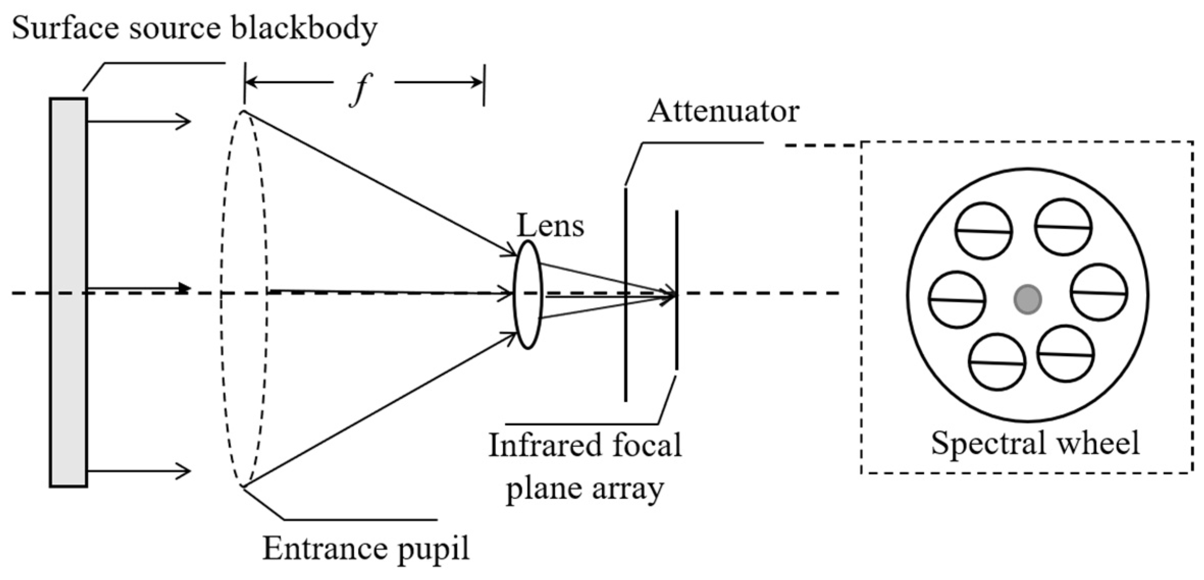
There are several radiometric calibration configurations used in infrared imaging systems [14,15]. The two most commonly used calibration configurations are near-collimating optics configuration and near-extended-source (NES) configuration. A near-collimating optics configuration performs radiometric calibration by expanding a collimated beam from a cavity blackbody, with incident radiation from a smaller source also filling the entry pupil. This configuration is costly and has constraints in laboratory settings. In the NES configuration, a surface blackbody is positioned at the system’s entrance pupil, ensuring that the incident radiation covers the entry pupil during calibration. This method offers high accuracy and effectively minimizes external influences such as atmospheric attenuation. However, due to manufacturing limitations, the dynamic temperature range of the extended area blackbody is limited, rendering the NES configuration unsuitable for wide dynamic range radiometric calibration.
The near-extended-source configuration is used in the study. Figure 1 shows the radiometric calibration diagram.

Figure 1.
The radiometric calibration diagram.
Assuming that the infrared imaging system operates within the linear response range, the relation between the radiance at the system’s entrance pupil and the gray level of the output infrared image is linear [16,17,18]. The expression is given as follows:
where represents the gray level, is the integration time, represents the total system gain that takes the electrical and optical systems into account, and is the gray level offset term of the detector, which is caused by internal factors such as dark current. represents the internal equivalent stray radiation of the system, which can be conceptualized as equivalent radiation from the optical system’s incident upon the entrance pupil. Calculating the stray radiation at the entrance pupil facilitates the comparison of the relative magnitudes between stray radiation and the target radiance, especially when the dynamic range is altered. It endows the stray radiation term with a tangible physical significance. is the target radiance, which can be calculated using Planck’s blackbody radiation formula [1]. It can be expressed as
where is the emissivity of the blackbody, is the Planck constant with the value of , is the speed of light with the value of , is the Boltzmann constant with the value of , is the wavelength of radiation, and is the Kelvin temperature.
When an attenuator is interposed between the detector and the optical lens of the infrared imaging system, it linearly diminishes all incoming radiation. Concurrently, the stray radiation associated with the attenuation is incorporated into the radiometric calibration model. Equation (2) can be rewritten as
is the transmittance of the attenuator. is the equivalent radiation from the attenuator, and it can be viewed as the attenuator’s equivalent radiation incident from the entrance pupil, as in . The max value of is determined by the number of used attenuator gears in the infrared system. The above physical quantities are for a single pixel in the infrared FPA detector. Nonuniformity correction can be performed in the gray-level domain based on Equation (3).
Equation (3) is changed to a function of the radiance concerning the gray level. The expression is given as follows:
Equation (4) is usually solved by collecting blackbody images at multiple operating points and calculating their theoretical radiance. The coefficients , , , , and of radiance concerning integration times and gray levels are obtained. Based on Equation (4), nonuniformity corrections can be performed in the energy domain.
2.2. Dynamic Adjustment Mechanism
The goal of the dynamic adjustment mechanism is to keep the detector in the optimal dynamic range while maintaining a satisfactory corrective effect in the output images of the system. The linear calibration range with high calibration accuracies is used as the linear dynamic range of the system. It is derived based on Equation (4), a known linear model. When the range of the gray level and the integration time are known, Equation (4) can be used to describe the relation of the radiance concerning integration times and gray levels. A sample of the relation is shown in Figure 2.
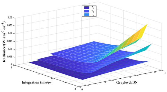
Figure 2.
The relation of radiance concerning the attenuator transmittance, integration time, and gray level of the infrared image.
In Figure 2, the magnitude relation of the transmittance is . The stray radiation of the uncalibrated attenuator at a specific ambient temperature can be estimated using Equation (2) [19]. The range of the integration time is determined by the system’s settings. The gray-level range is established through calibration and dynamic processes. The lower limit of the dynamic gray range increases as the attenuator’s transmittance descends. Both integration times and gray levels are normalized for better exhibition.
As the attenuator’s transmittance decreases, the curvature of the surface increases, indicating a broader dynamic range of radiance. Given a fixed integration time, a lower attenuator transmittance results in a reduced gray-level range detectable by the system. Both adding an attenuator and adjusting integration times are effective methods for expanding the system’s dynamic range.
The operating points in the linear calibration range may not have optimal correction effects, and this is due to the influence of the signal-to-noise ratio (SNR) [20,21]. System background noise primarily includes photon, dark current, and readout circuit noise [22]. Photon noise is composed of stray radiation noise from the optical lens and the attenuator. Consequently, SNR can be expressed as
For a certain infrared imaging system and a certain target, the values of , , and will vary with the adjustment of integration times and the transmittance of the attenuator. is associated with the intrinsic properties of the attenuator. and are determined via the characteristics of the detector and the readout circuits of the system. Figure 3 is a graphical representation that illustrates the general trend based on Equation (5). Figure 3a describes the relation between SNR and integration time at two attenuator gears. is determined when the attenuator is chosen. In the optimal dynamic range of the system, the SNR will increase with an increase in integration times. Points A, B, C, and D are four different operating points. When the SNR is low at point A, it can be enhanced by increasing the integration time. When the gray value reaches the upper limit of the system’s linear response range at point B (as shown by the dotted line in Figure 3a, if the upper limit is not reached, SNR can continue to increase by increasing the integration time), a lower transmittance of the attenuator is switched to in the optical path at point C. Although this step reduces SNR, a higher value can be achieved by increasing the integration at point D.
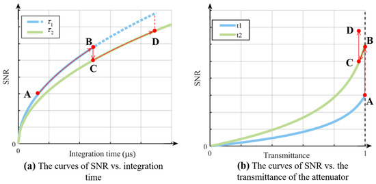
Figure 3.
The curves of SNR vs. integration time and SNR vs. the transmittance of the attenuator.
Figure 3b describes the relation between SNR and the transmittance of the attenuator at two integration times. When the integration time is determined, noise received by the detector will increase due to the stray radiation introduced by the attenuator. The stray radiation of the attenuator will increase with a decrease in transmittance. The steps from A to D describe the same physical process as that in Figure 3a.
Different operating points can be achieved by setting the integration time and the attenuator. In the process of dynamic range adjustment, three variables can be taken into account: minimum gray level , maximum gray level , and average gray level of the infrared image. These three variables are compared with the optimal dynamic range of the system. There are three situations:
where represents the subset of the linear response range of the system, with different operating points corresponding to different :
- (1)
- When , the integration time should be increased until . If the integration time reaches the maximum value of the system’s setting and is still less than , the attenuator with higher transmittance is switched into the optical path.
- (2)
- When , the system is within the optimal dynamic range. No further action is needed.
- (3)
- When , the integration time should be decreased until . If the integration time reaches the minimum value of the system’s setting and still exceeds , the attenuator with lower transmittance is switched into the optical path.
3. Nonuniformity Correction Method Based on Unsupervised Learning
Existing nonuniform correction algorithms typically operate in the gray-level domain. Adjustments of the system operating points, such as the transmittance of attenuators and/or integration times, will change the gray level of infrared images captured from the same scene as well. The adjustments result in outputted gray-level jumps, complicating the post-processing of the infrared system, such as target detection, tracking, and recognition. Switching from the gray-level domain to the energy domain can solve the problem effectively. However, the energy-domain nonuniformity correction approach usually needs to accurately obtain blackbody temperatures, emissivities, and wavebands. The deviation from the ground-truth value will affect calibration accuracy.
In reference [16], Equation (4) is solved by utilizing the loss function and backpropagation of the BP network. The iterative process of the coefficient’s learning network converges to the global optimal solution. The algorithm uses the theoretical radiance calculated from the blackbody temperature as the regression goal for training the coefficient’s learning network. The feedback value is defined as the difference between theoretical radiance and the network-predicted value. During training, the calibration points at the same blackbody temperature will cluster together, and the distance between the network-predicted value and theoretical radiance is minimized. This is a result of all calibration points being correlated by Equation (4), and radiance is calculated via blackbody temperatures, emissivities, and wavebands.
Based on the above, the calibration points of the same temperature will automatically cluster together according to the physical correlation; thus, theoretical radiance can be replaced by the average predicted value at the same blackbody temperature settings. This clustering process is similar to the K-means clustering mechanism [23,24]. Figure 4 illustrates the schematic diagram of blackbody radiance clustering. Each horizontal line represents a cluster center. T1~T3 are unknown blackbody temperature settings. Each dot represents a specific operating point in the figure. In each cluster, the average position is determined using the same specific blackbody temperature settings. The selection of the temperature should be within the dynamic range’s boundary, and the interval should not be small; otherwise, the calibration’s accuracy would be affected.
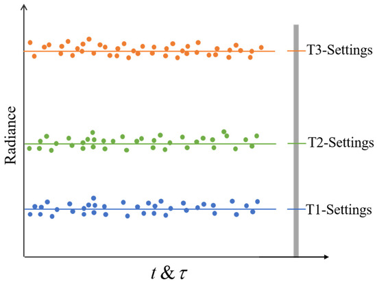
Figure 4.
The schematic diagram of blackbody radiance clustering.
Consequently, a nonuniformity correction approach based on unsupervised learning is proposed. Each operating point will not be labeled during the training process. The clustering center is determined by the average predicted value generated using Equation (4) with respect to calibration data at the same specific blackbody settings. In the clustering process, the center of each cluster continuously shifts until the distances between the cluster’s operating points and the center are minimized. The number of clustering centers corresponds to the calibration’s blackbody temperature settings. The goal of the calculation is to minimize the differences in the network-predicted value and the average predicted value. Thus, Equation (4) can be rewritten as
where , , , , and are learned from the unsupervised coefficient learning network. is the predicted value of the specific operating point. The expression of is given as follows:
where is the number of calibration points at the same specific blackbody temperature, (i, j) is the pixel coordinate of the detector, is the serial number, and and are the rows and columns of the infrared FPA, respectively.
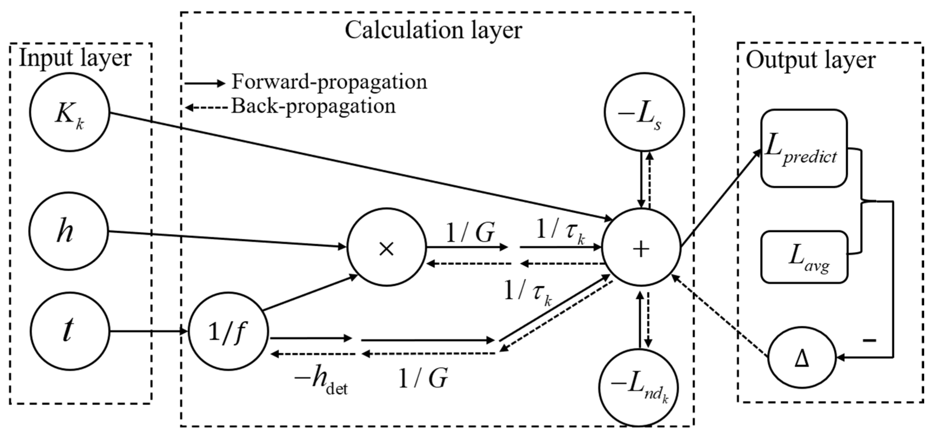
The mechanism of the unsupervised clustering algorithm and coefficient learning model is shown in Figure 5. The forward network structure for regression is first built and divided into three layers: the input layer, the calculation layer, and the output layer. The input layer consists of the gray level of the blackbody image and its corresponding integration time and attenuator selection coefficient . is the enable signal: the selected attenuator is 1, and the rest are 0. The calculation layer is based on Equation (7). The output layer is composed of the average predicted value of all calibration data at the same specific blackbody temperature settings. Once the initial values for each coefficient in Equation (3) of the learning network are set, the initial average predicted value is established. The loss function is defined as the sum of the squares of the relative errors between the predicted value and the average predicted value. The equation is given as follows:
where is the sequence number of the calibration points and is the total number of calibration points. To determine the direction of the gradient’s descent, the chain rule is applied to compute the partial derivative of each coefficient. During the gradient descent process of the neural network, solving the molecular section results in the formation of a high-order term. It will affect both the convergence of the gradient descent and the stability of the network’s training. Thus, the reciprocal of the coefficients in the denominator in Equation (7) is regarded as a whole term. The equation is given as follows:
where is obtained as follows:

Figure 5.
The diagram of the unsupervised learning model.
Then, the learning direction of the coefficients is obtained as follows:
It should be noted that the training goal is set as the average of the predicted value and not the true radiance value; thus, the predicted value can only be used for nonuniformity corrections and cannot be regarded as the radiance value. The predicted value and the radiance value have a linear relation at the same temperature, which can be written as
Linear coefficients and represent how the predicted value maps to the radiance value. Linear coefficients and can be determined by using at least two known blackbody temperature settings.
4. Experiment and Analysis
4.1. The Experimental System Setup
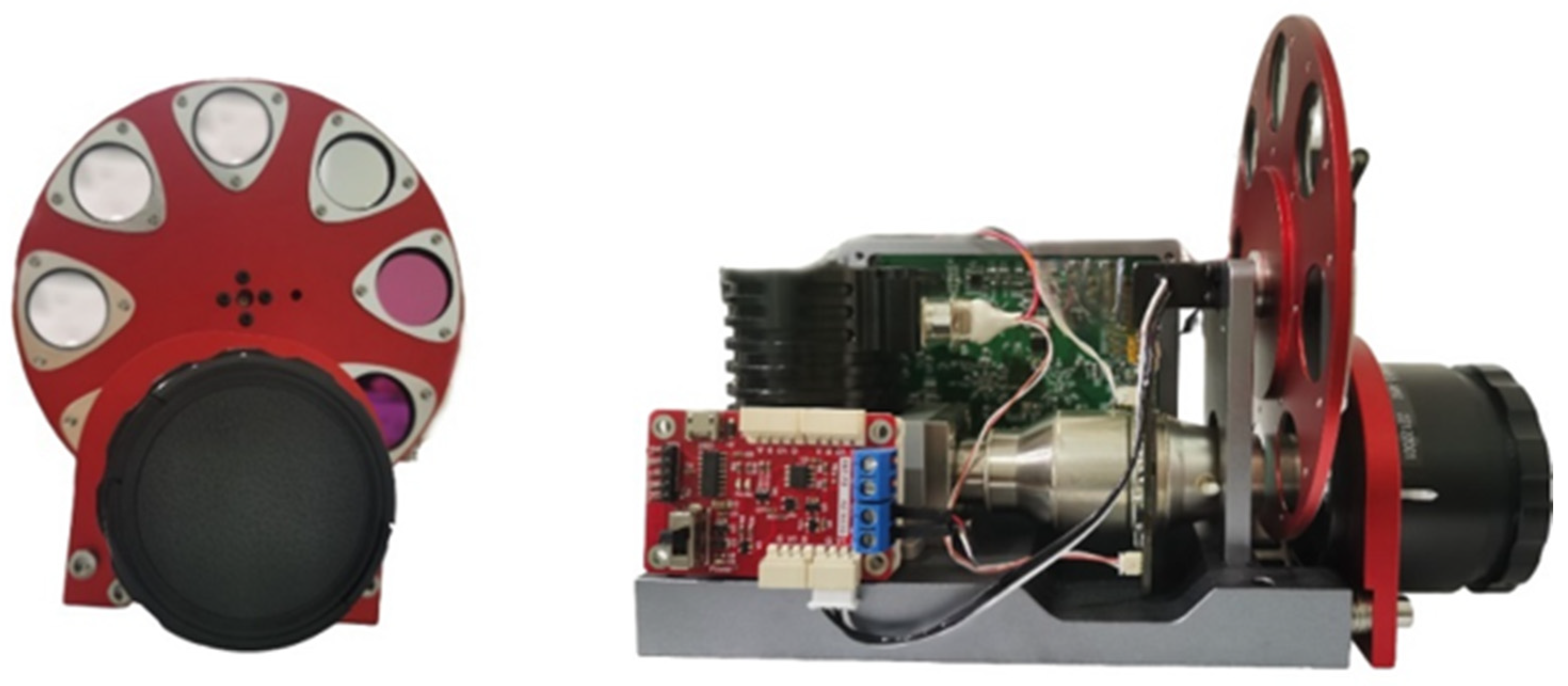
The proposed method is based on the derived infrared physical model that applies to the entire infrared spectrum, including short, medium, and long waves. In the experiment, the medium wave (MW) band is selected for verification. The experimental MW infrared imaging system consisted of an optical lens, an attenuator spectrum wheel, and an infrared detector. Table 1 lists the main parameters of the system. The attenuator is positioned between the optical lens and the detector, which is designed based on a six-vacancy spectral wheel. Figure 6 shows a picture of the infrared imaging system. The infrared system and the host computer communicate using an asynchronous serial format via RS422. The FPA provides a 14-bit digital output. The DCN 1000 H4 blackbody, manufactured by the HGH, is chosen as the experimental blackbody. This blackbody has an emissivity of 0.99 within the 1–14 µm waveband. Its temperature accuracy is 0.0005 °C, with an operating temperature range from −40 to 150 °C. It is necessary to note that in order to prevent defocusing when switching between different attenuator gears during real infrared image capture, the thickness of the attenuator with different transmittance values needs to be specifically designed in order to ensure equal optical path differences. If the thickness of the attenuators is not designed, manual focus adjustment is required for the infrared imaging system.

Table 1.
The main parameters of the infrared system.

Figure 6.
The picture of the infrared system.
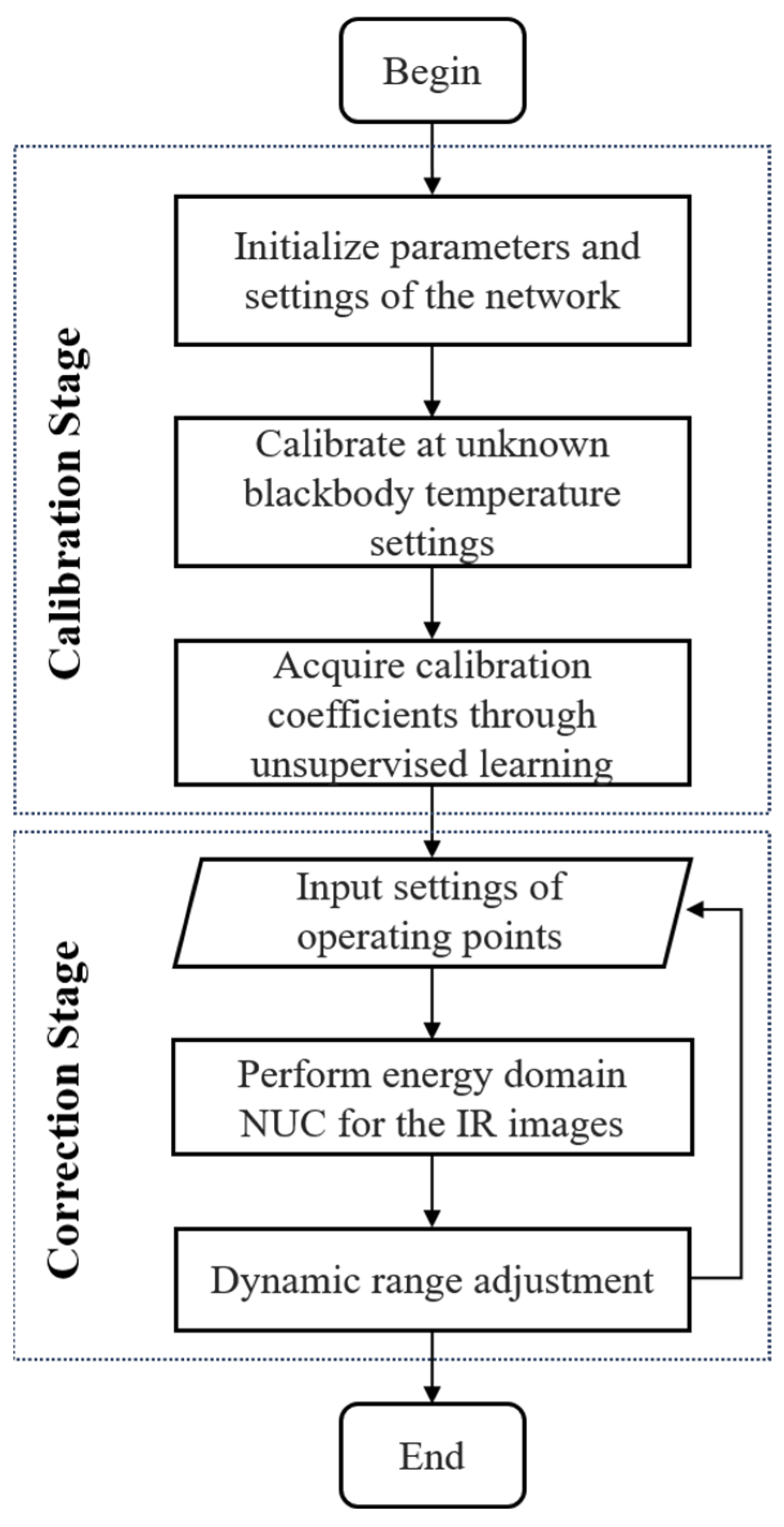
The experimental flow of the nonuniformity correction algorithm is shown in Figure 7. There are two stages in the experiment procedure. One is the calibration stage, which acquires the coefficients of the correction model and only needs to be carried out once in the experiment. The other is the correction stage, which implements the nonuniformity correction of the different real scene images. In the calibration stage, the system coefficients , , , , and from Equation (7) are initialized first. Simultaneously, the learning rate is set for the coefficient learning network. Then, a unified database is established by collecting different operating points at different blackbody temperatures. After multiple iterations of unsupervised training, the energy-domain infrared nonuniformity correction model that adapts to the changes in integration time and attenuators is acquired. This process also determines the system’s optimal dynamic range. In the correction stage, the trained correction network is deployed to the VS-based infrared image acquisition platform in order to evaluate the correction effect on real-scene images. Then, the operating point’s settings are inputted, and energy-domain nonuniformity corrections are performed for real scene images. Finally, dynamic range adjustments are performed in order to obtain the best correction range for the infrared system.
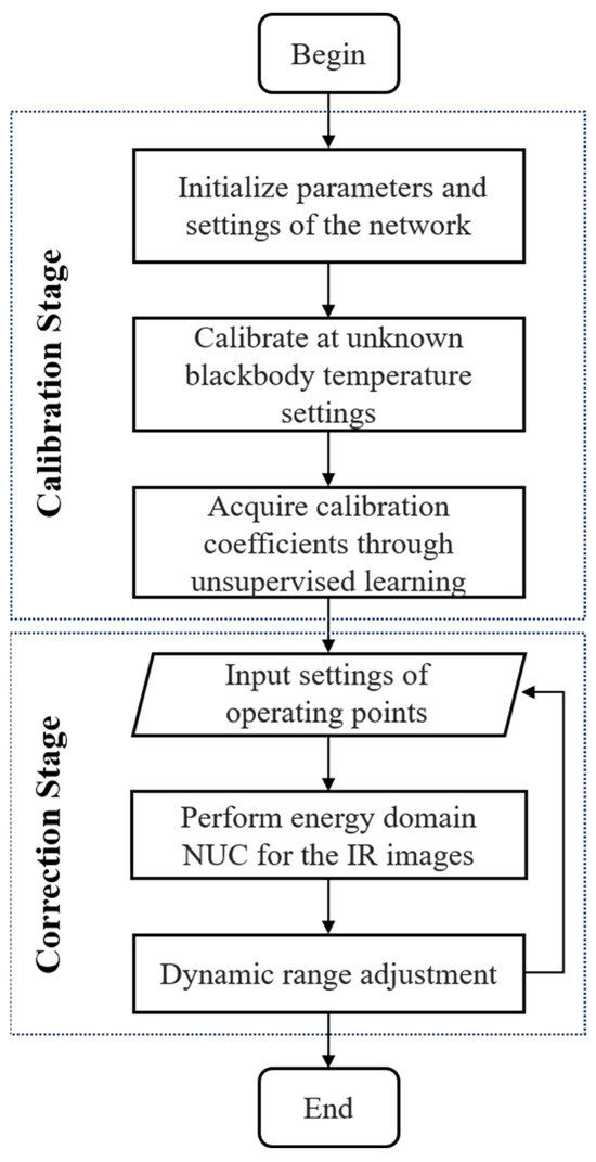
Figure 7.
The flow chart of the proposed method.
4.2. Unsupervised Learning Process
Firstly, blackbody calibration is performed on the infrared imaging system. Then, a unified database is created by gathering the blackbody images of four integration times and two unknown temperature points under each attenuator gear in the optimal dynamic range. The ambient temperature is steady at 29 °C during the process of calibration.
In the experiment, two categories of attenuation information are set. Filter I is the no-lens gear. The nominal transmittance of Filter II is 88% within the 3–5 waveband. The integration time is set to 960 , 1280 , 1600 , and 1920 . The blackbody temperature is 30 °C and 60 °C under Filter I. Moreover, 40 °C and 70 °C are the selected blackbody temperatures under Filter II. The input of the dataset consists of the normalized and and the filter selection coefficients ( and ). The output of the dataset consists of the predicted value . The dataset is set as follows:
where is the maximum gray level of the blackbody images, is the maximum integration time, and is the maximum predicted value.
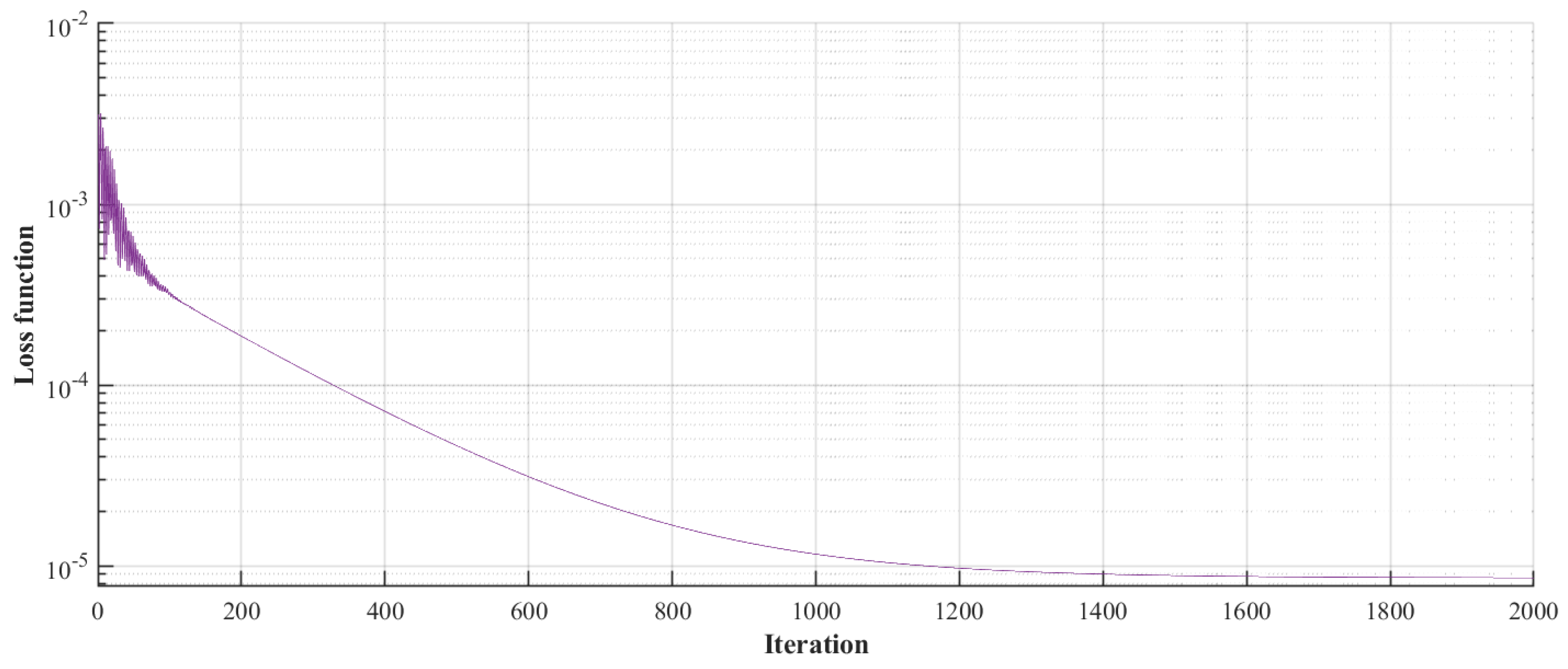
Establishing the unsupervised coefficient learning network according to Figure 5, the coefficients of the correction model are acquired by the iteration’s training. The learning rate is set to 0.01. The clustering algorithm is significantly influenced by the initial clustering centers. In the initial training process, the center of each cluster continuously shifts to find an optimal center of clustering, and the loss function curve fluctuates greatly. After multiple iterations, the loss function begins to converge, and training is stopped when the value of the loss function becomes stable. The training process is shown in Figure 8, and the value of the loss function is 8.5 × 10⁻⁶.
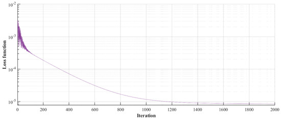
Figure 8.
Training curve of the loss function value.
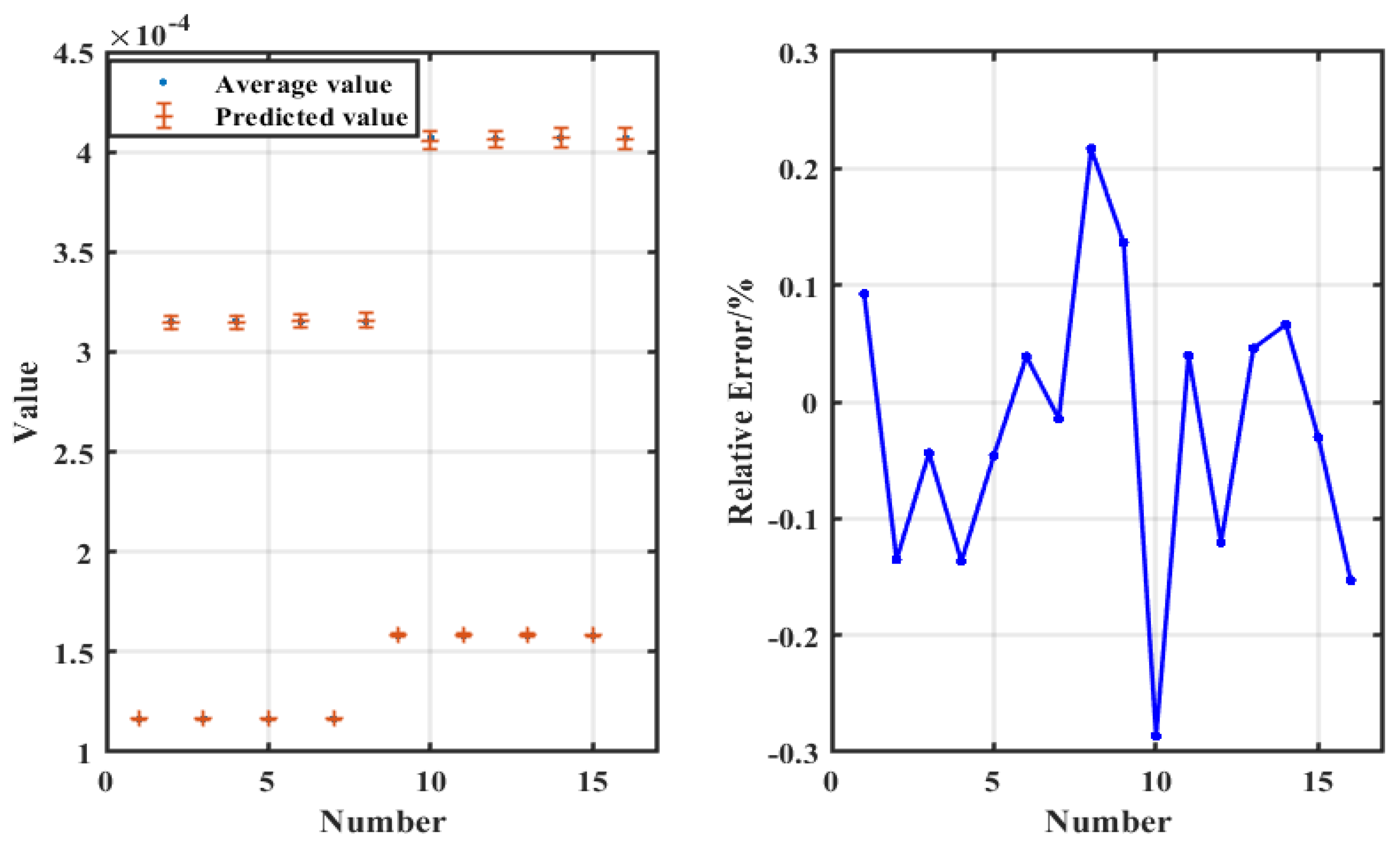
Figure 9 presents the learning results. Numbers 1 to 8 represent the operating points under Filter I, while numbers 9 to 16 represent those under Filter II. The left graph illustrates the degree of fitting between the predicted value and the average value at the same blackbody temperature. The calculation method of the error bars of the predicted values follows the “3” criterion. The graph on the right depicts the relative error for the corresponding operating points. As observed from the graphs in Figure 9, each operating point can be regressed to the goal. The relative fitting error of the corresponding points does not surpass 0.3%.

Figure 9.
The fitting result of the 16 operating points and the relative error of the corresponding point.
After training, the coefficients for the nonuniformity correction model are determined. Table 2 presents the coefficients of the model, while Table 3 provides the equation of the model. is the predicted value of the total system gain, is the predicted value of the gray-level offset, is the predicted value of the internal equivalent stray radiation, is the predicted value of the equivalent radiation from the attenuator, and is the transmittance of the attenuator. It should be noted that the training goal is set as the average of the predicted value and not the radiance value; thus, the predicted value of the model’s coefficients can only be used for nonuniformity correction and cannot be directly used to represent true radiance. The linear response range of the system is 2000~12,000 DN.
Table 2.
Coefficients of the nonuniformity correction models.
Table 3.
Calibration formula of the methods.
4.3. Comparison and Analysis of Experimental Results
Upon the completion of the calibration process, the coefficients of the model can be used to correct the nonuniformity of the real infrared scenes. During the image-collecting process, the operating points are changed by adjusting integration times and attenuator settings. The comparison and analysis of experimental results are as follows.
4.3.1. Comparison of Image Display Results Under Different Integration Times
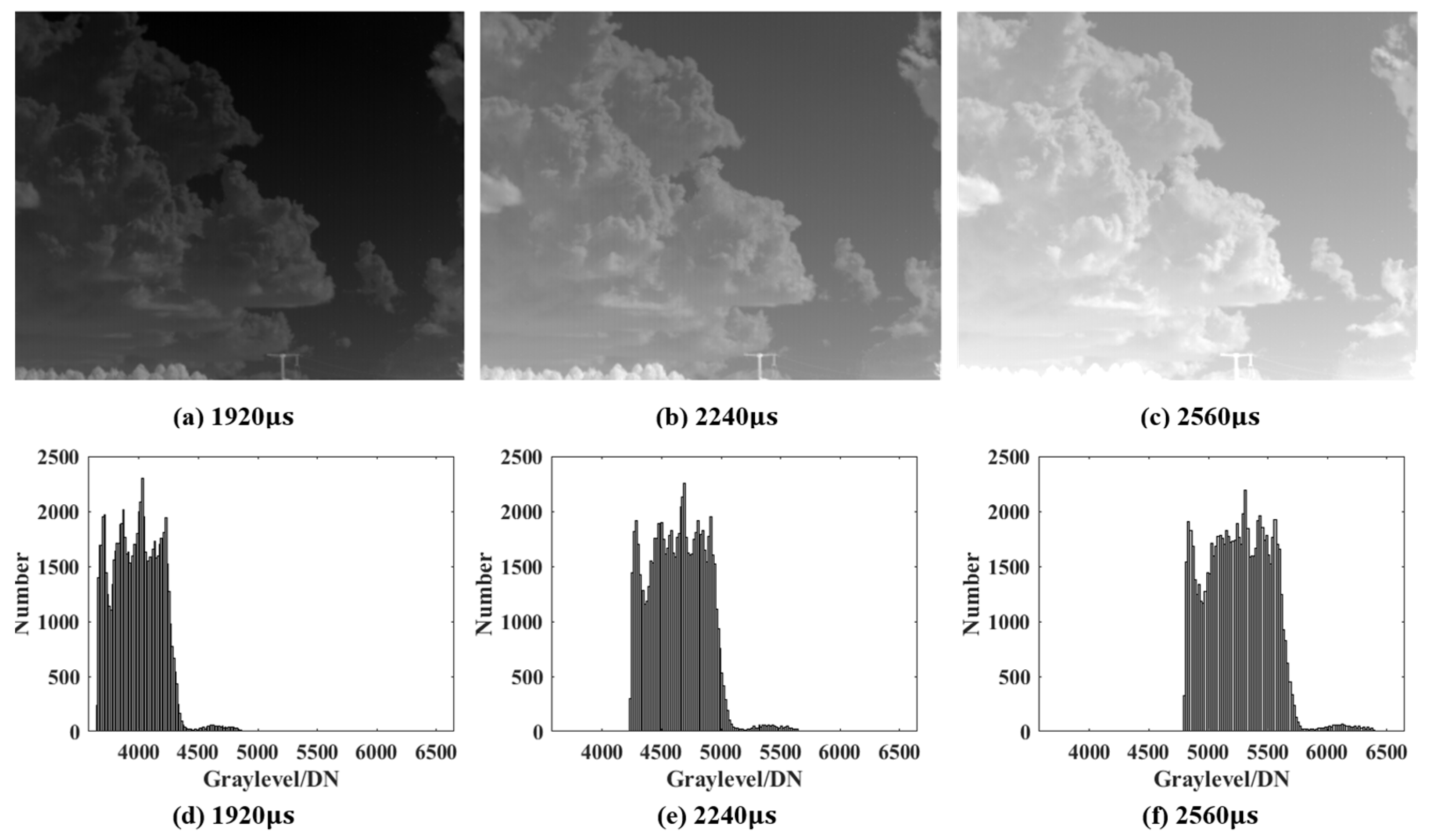
Firstly, Filter I is chosen by rotating the spectral wheel. Then, the integral time was adjusted to 1920 , 2240 , and 2560 . For each setting, nonuniformity correction was performed using the conventional two-point correction algorithm for the same scene. Figure 10 presents the comparison chart along with the corresponding gray histograms.
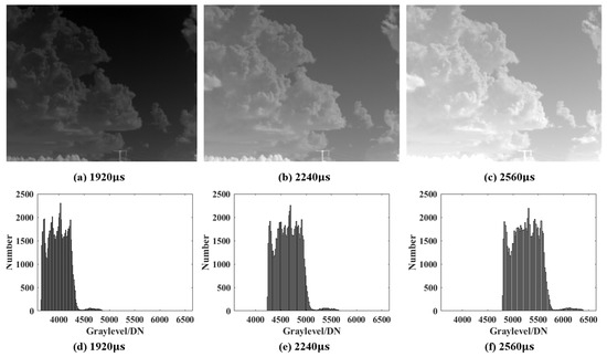
Figure 10.
The images corrected by the two-point correction algorithm and their corresponding gray histogram under different integration times.
As observed in Figure 10d–f, the distribution of the gray histogram shifts noticeably to the right. The average gray levels of the images in Figure 10a–c are 3986 DN, 4640 DN, and 5257 DN. The corrected image is brighter relative to an increase in integration time. The relative change in the mean gray level of Figure 10b,c relative to Figure 10a is 16.41% and 31.89%, respectively. This indicates obvious changes in the image’s brightness in the display domain.
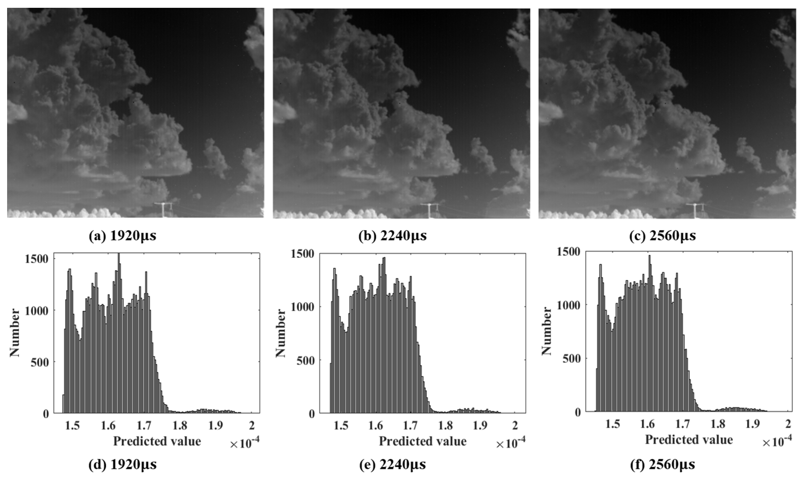
Under the same integration time settings, Figure 11 displays the energy-domain image and its corresponding histogram relative to the proposed energy-domain algorithm.
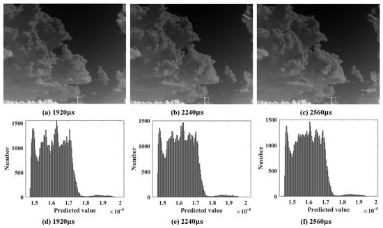
Figure 11.
The images corrected using the proposed method and their corresponding histogram under different integration times.
As shown in Figure 11d–f, the distribution of gray histograms barely moves. The average image values in Figure 11a–c are 1.6113 × 10⁻⁴, 1.6062 × 10⁻⁴, and 1.5911 × 10⁻⁴. The relative variation in the mean value relative to Figure 11a is 0.32% and 1.25%. There is no significant change in the three energy-domain images. The proposed method results in more stable corrected images compared to the two-point method when integration time changes and the attenuator is fixed.
4.3.2. Comparison of Image Display Results Under Different Transmission Attenuator Gears
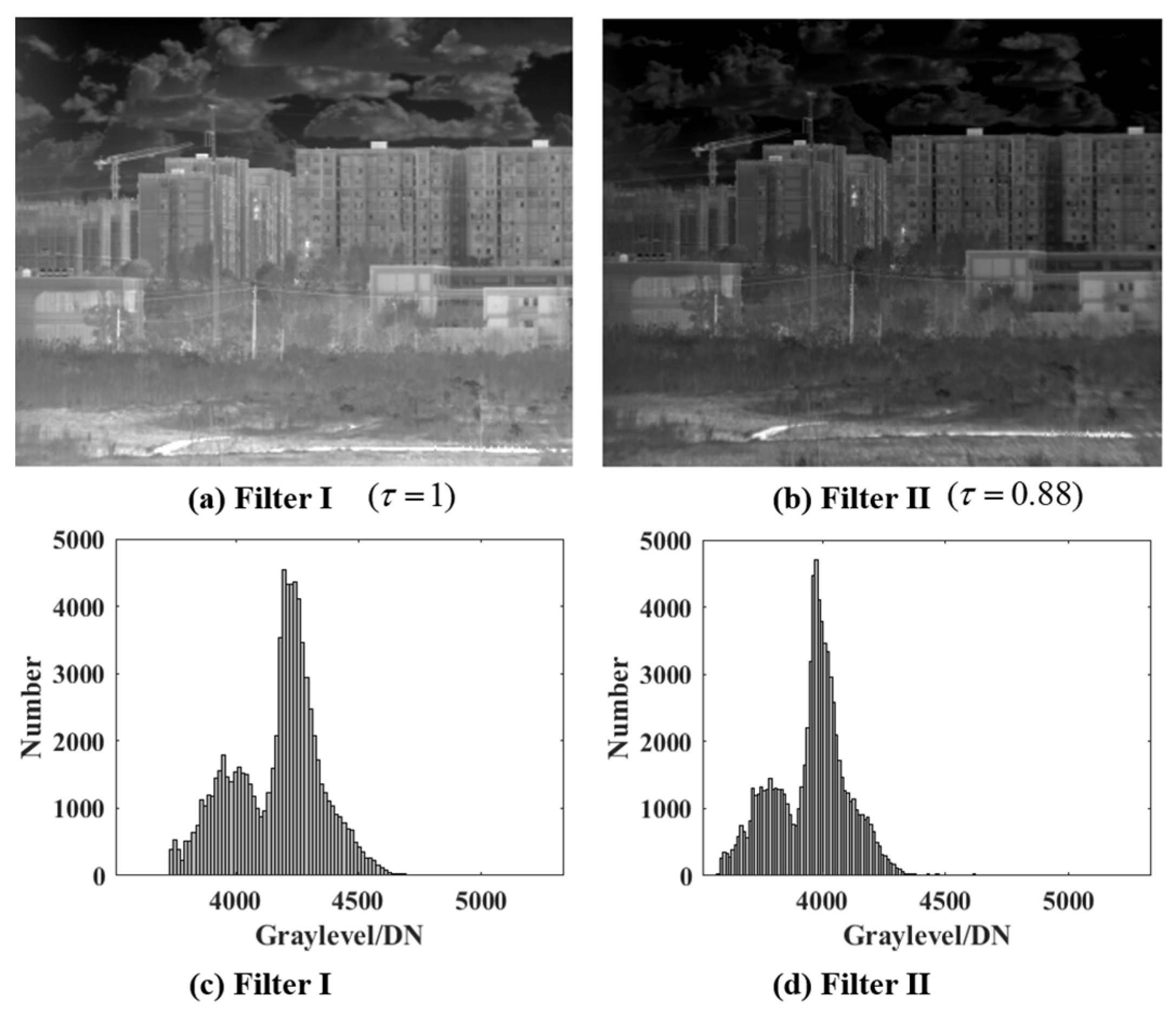
The integration time is set to 1920 , and the spectral wheel is rotated to choose Filter I and Filter II in turn. Then, real scene images are collected, and the conventional two-point correction method is used. The effects are shown in Figure 12.

Figure 12.
The images corrected by the two-point correction algorithm and their corresponding gray histogram under different attenuator gears.
As observed in Figure 12a,b, the corrected image under Filter I’s gear is brighter than the corrected image under Filter II’s gear. The gray level’s distribution shifts noticeably to the left in Figure 12c,d. The average gray levels of the images are 4172 DN and 3955 DN, respectively. The relative change in the mean gray level of Figure 12b relative to Figure 12a is 5.20%.
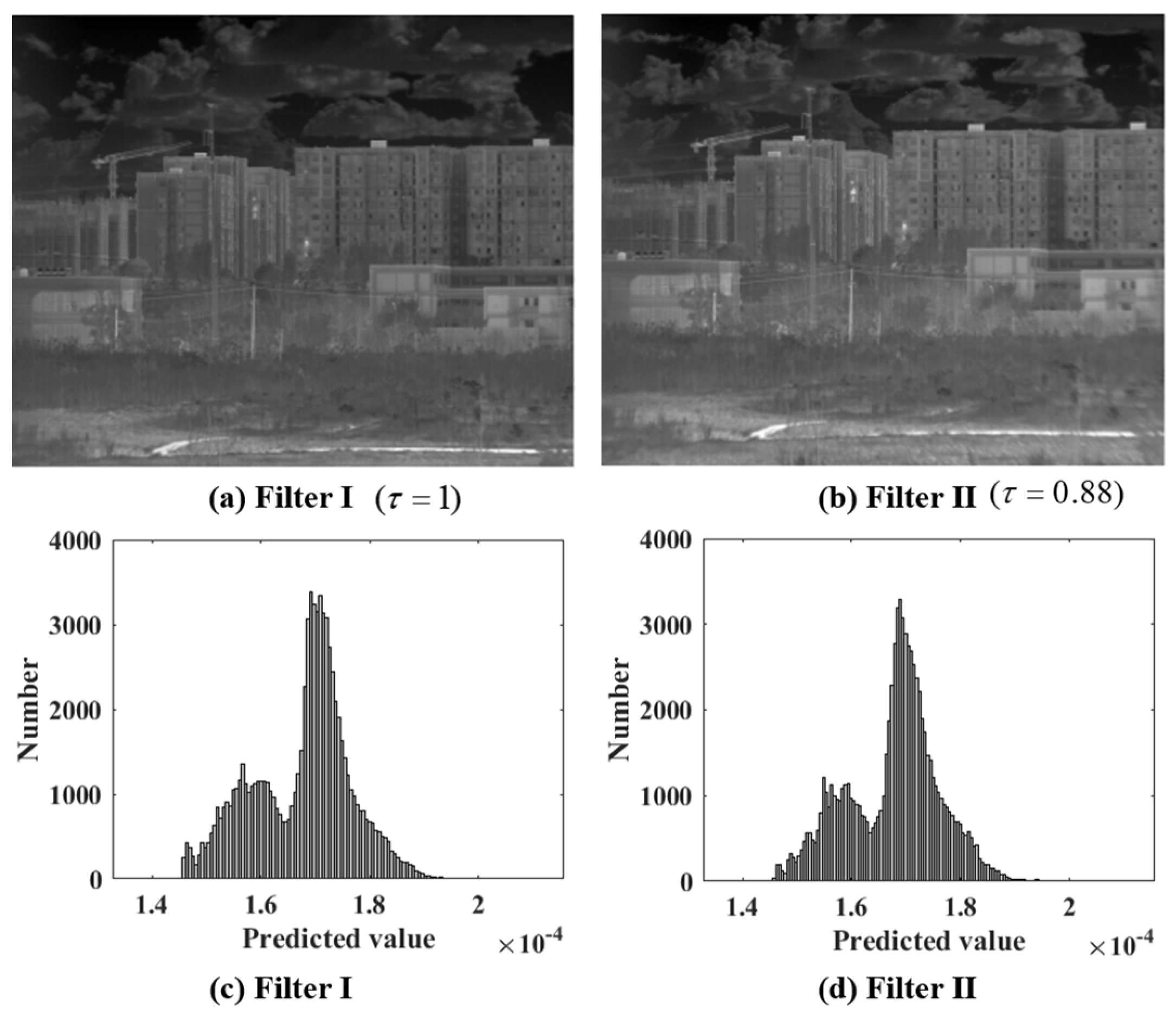
The nonuniformity correction results of the proposed method under the same settings are illustrated in Figure 13.
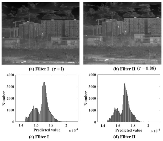
Figure 13.
The images corrected by the proposed method and their corresponding histograms under different attenuator gears.
In Figure 13a,b, the values of the corrected images under Filter I’s gear and Filter II’s gear have no obvious difference. The gray level’s distribution exhibits no obvious changes, and this is also observed in Figure 13c,d. The average image values in Figure 13a,b are 1.6780 × 10⁻⁴ and 1.6785 × 10⁻⁴, respectively. The relative change in the average value of Figure 13b relative to Figure 13a is 0.03%. The proposed method results in a more stable output of the corrected images compared to the two-point correction algorithm when integration time is fixed and the attenuator changes.
4.3.3. Image Display Results at Uncalibrated Operating Points
Traditional calibration-based nonuniformity correction algorithms, such as the one-point, two-point, and multi-point correction algorithms, need to calibrate operating points in advance. The proposed method can perform the nonuniformity correction of the image at any operating point within the optimal dynamic range. Figure 14 displays three images that are captured at the same scene relative to different integration times. The operating point with an integration time of 1920 is calibrated. The operating points with the integration times of 1472 and 2368 have not been calibrated.
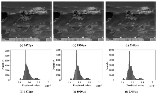
Figure 14.
The images corrected by the proposed method and their corresponding histogram under uncalibrated operating points and a calibrated operating point.
From Figure 14a to Figure 14c, the result shows there is no discernible increase in fringe noise or change in predicted value in the corrected image. The gray level’s distribution has no obvious changes, as observed in Figure 14d–f. The average image value of the three images is 1.5693 × 10⁻⁴, 1.5758 × 10⁻⁴, and 1.5708 × 10⁻⁴, respectively. The relative change in the mean value of Figure 14b,c relative to Figure 14a is 0.41% and 0.10%, respectively. The proposed method results in a similar correction effect under the calibrated and uncalibrated operating points.
4.3.4. Dynamic Adjustment Process
Figure 15 shows the three images acquired with different operating points. As depicted in Figure 15a, significant fringe noise is observed in the captured image (average SNR: 8.074; background noise: 0.014) when Filter II is chosen with an integration time of 640 . Then, the dynamic adjustment mechanism begins operation, and the system progressively increases the integration time. Figure 15b illustrates that a small amount of fringe noise remains in the image (average SNR: 10.363; background noise: 0.011) after the integration time reaches its maximum value of 2560 . This indicates that the image’s gray level has not yet reached the lower threshold of the optimal dynamic range under Filter II. Subsequently, as shown in Figure 15c, the spectral wheel rotates, and the Filter I gear is chosen. The captured image (average SNR: 10.800; background noise: 0.010) exhibited no significant fringe noise, showing that the infrared imaging system is functioning within its optimal dynamic range.
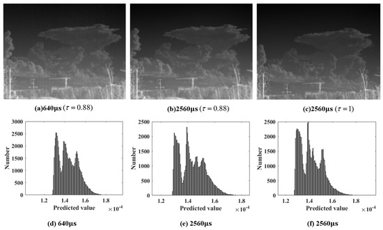
Figure 15.
Schematic diagram of the dynamic adjustment process.
4.3.5. Summary of Comparative Analysis
The above experiments verify that the traditional nonuniformity correction method changes the output gray level when the integration time and attenuator change. Moreover, the proposed method maintains uniform and stable outputs when the dynamic range changes, and it does not need accurate blackbody temperature, emissivity, and waveband values. This is because the proposed method converts gray-level domain corrections into energy domain corrections. The summarized table for performance comparisons with the traditional method is shown in Table 4.
Table 4.
Performance comparison.
5. Conclusions
This study proposes an energy-domain IR NUC method adapted to dynamic range changes based on unsupervised machine learning. Firstly, an energy-domain infrared physical model is established, and a dynamic adjustment mechanism is introduced to ensure that the system operates within the optimal dynamic range. Then, by exploring the inherent physical correlations within the calibration dataset, a unified database is generated by integrating gray levels, integration times, and attenuator information. Without knowing the calibration’s blackbody temperature, emissivity, and waveband, the coefficients of the correction model are learned based on the clustering-based unsupervised learning methodology by setting the average predicted value of the same blackbody temperature as the learning goal. The experiment’s results show that the trained correction network maintains uniform and stable image outputs during the adjustment of the integration time and attenuator, and it keeps the infrared system operating within the optimal dynamic range. The maximum change in the image corrected by the proposed algorithm is 1.29%.
A potential application of the proposed method is the calibration-based radiation measurement. The radiation calibration errors are partially introduced by the mismatch between the calculated theoretical radiance and true radiance. One reason for this phenomenon is that the actual blackbody temperature might be different from the preset temperature due to the equipment’s accuracy and the insufficient time elapsed to reach the temperature balance. The other reason is that the emissivity of the blackbody is usually treated as a fixed value in the calculation but, actually, it conforms to a specific spectral response within the working waveband. The proposed method avoids using the exact blackbody parameters during the clustering-based unsupervised training stage and provides a new solution as a reference.
Author Contributions
Conceptualization, T.L.; methodology, T.L. and X.L.; software, T.L. and X.L.; validation, T.L. and X.L.; writing—original draft preparation, T.L.; writing—review and editing, T.L., X.L., S.L. and Y.X. All authors have read and agreed to the published version of the manuscript.
Funding
This research received no external funding.
Data Availability Statement
The raw data supporting the conclusions of this article will be made available by the authors upon request.
Conflicts of Interest
The authors declare no conflicts of interest.
References
- Zhou, S.C. Introduction to Advanced Infrared Optoelectronic Engineering, 1st ed.; Science Press: Beijing, China, 2018; pp. 8–28. [Google Scholar]
- Harris, J.G.; Chiang, Y.M. Nonuniformity correction using the constant-statistics constraint: Analog and digital implementations. Proc. SPIE-Int. Soc. Opt. Eng. 1997, 3061, 895–905. [Google Scholar]
- Marcotte, F.; Tremblay, P.; Farley, V. Infrared camera NUC and calibration: Comparison of advanced methods. In Infrared Imaging Systems: Design, Analysis, Modeling, and Testing XXIV; SPIE: San Diego, CA, USA, 2013; Volume 8706, pp. 17–26. [Google Scholar]
- Sofu, B.; Sakaryal, D.U.; Akin, O. Comparison of Non-Uniformity Correction Methods in Mid-wave Infrared Focal Plane Arrays of High Speed Platforms. In Applications of Digital Image Processing XLI; SPIE: San Diego, CA, USA, 2018; pp. 20–31. [Google Scholar]
- Liu, Y.M. High-precision combined nonuniformity correction method based on local constant statistics. Acta Photonica Sin. 2019, 48, 0604002. [Google Scholar] [CrossRef]
- Yu, Y.; Lee, B.G.; Pike, M.; Zhang, Q.; Chung, W.Y. Deep learning-based RGB-thermal image denoising: Review and applications. Multimed. Tools Appl. 2024, 83, 11613–11641. [Google Scholar] [CrossRef]
- Peng, Y.; Xu, B.; Zhang, C. Infrared Image Non-uniformity Correction Based on Joint Surface of Radiation and Environment Temperature. Opto-Electron. Eng. 2016, 43, 89–94. [Google Scholar]
- Friedenberg, A.; Goldblatt, I. Nonuniformity two-point linear correction errors in infrared focal plane arrays. Opt. Eng. 1998, 37, 1251–1253. [Google Scholar] [CrossRef]
- Scribner, D.A.; Sarkady, K.A.; Caulfield, J.T.; Kruer, M.R.; Gridley, C.J. Nonuniformity correction for staring IR focal plane arrays using scene-based techniques. In Infrared Detectors and Focal Plane Arrays; SPIE: San Diego, CA, USA, 1990; pp. 224–234. [Google Scholar]
- Cui, K.; Chen, F.S.; Su, X.F.; Cai, P. Adaptive non-uniformity correction method for IRFPA with integration time changing. Infrared Laser Eng. 2017, 46, 77–83. [Google Scholar]
- Shen, S.W.; Lin, C.Q. An Adaptive Adjustment Algorithm for Dynamic Range of Infrared Camera Based on Kalman. Infrared 2017, 38, 5. [Google Scholar]
- Chen, N.; Zhang, J.; Zhong, S.; Ji, Z.; Yao, L. Nonuniformity Correction for Variable-Integration-Time Infrared Camera. IEEE Photonics J. 2018, 10, 1–11. [Google Scholar] [CrossRef]
- Ochs, M.; Schulz, A.; Bauer, H.-J. High dynamic range infrared thermography by pixelwise radiometric self calibration. Infrared Phys. Technol. 2010, 53, 112–119. [Google Scholar] [CrossRef]
- Wolfe, W.L. Introduction to Radiometry; SPIE: San Diego, CA, USA, 1998. [Google Scholar]
- Nugent, P.W.; Shaw, J.A.; Pust, N.J. Radiometric calibration of infrared imagers using an internal shutter as an equivalent external blackbody. Opt. Eng. 2014, 53, 123106. [Google Scholar] [CrossRef]
- Li, T.; Lai, X.F.; Li, S.J.; Xia, Y.C.; Zhou, J.M.; Liao, S. Global optimization radiometric calibration method for an infrared system with a wide dynamic range. Appl. Opt. 2024, 63, 406–414. [Google Scholar] [CrossRef]
- Yao, T.; Jeseck, P.; Isabelle, P.; Camy-Peyret, C. A method to retrieve blackbody temperature errors in the two points radiometric calibration. Infrared Phys. Technol. 2009, 52, 187–192. [Google Scholar]
- Lee, H.; Oh, C.; Hahn, J.W. Calibration of a mid-IR optical emission spectrometer with a 256-array PbSe detector and an absolute spectral analysis of IR signatures. Infrared Phys. Technol. 2013, 57, 50–55. [Google Scholar] [CrossRef]
- Tian, Q.J.; Chang, S.T.; Qiao, Y.F.; He, F.Y. Radiometric calibration based on low-temperature area blackbody for infrared systems with high dynamic range. Guangzi Xuebao/Acta Photonica Sin. 2017, 46, 8. [Google Scholar]
- Tandra, R.; Sahai, A. SNR Walls for Signal Detection. Sel. Top. Signal Process. IEEE J. 2008, 2, 4–17. [Google Scholar] [CrossRef]
- Tandra, R.; Sahai, A. Fundamental limits on detection in low SNR under noise uncertainty. In Proceedings of the Wireless Networks, Communications and Mobile Computing 2005 International Conference, Wuhan, China, 23–26 September 2005. [Google Scholar]
- Ma, N.; Liu, S.; Li, J.Y. Analysis of spatial and temporal noise of infrared thermal imager. Laser Infrared 2017, 47, 717–721. [Google Scholar]
- Yousefi, B.; Ibarra-Castanedo, C.; Chamberland, M.; Maldague, X.P.V.; Beaudoin, G. Unsupervised Identification of Targeted Spectra Applying Rank1-NMF and FCC Algorithms in Long-Wave Hyperspectral Infrared Imagery. Remote Sens. 2021, 13, 2125. [Google Scholar] [CrossRef]
- Celebi, M.E.; Kingravi, H.A.; Vela, P.A. A Comparative Study of Efficient Initialization Methods for the K-Means Clustering Algorithm. Expert Syst. Appl. 2013, 40, 200–210. [Google Scholar] [CrossRef]


Disclaimer/Publisher’s Note: The statements, opinions and data contained in all publications are solely those of the individual author(s) and contributor(s) and not of MDPI and/or the editor(s). MDPI and/or the editor(s) disclaim responsibility for any injury to people or property resulting from any ideas, methods, instructions or products referred to in the content. |
© 2025 by the authors. Licensee MDPI, Basel, Switzerland. This article is an open access article distributed under the terms and conditions of the Creative Commons Attribution (CC BY) license (https://creativecommons.org/licenses/by/4.0/).