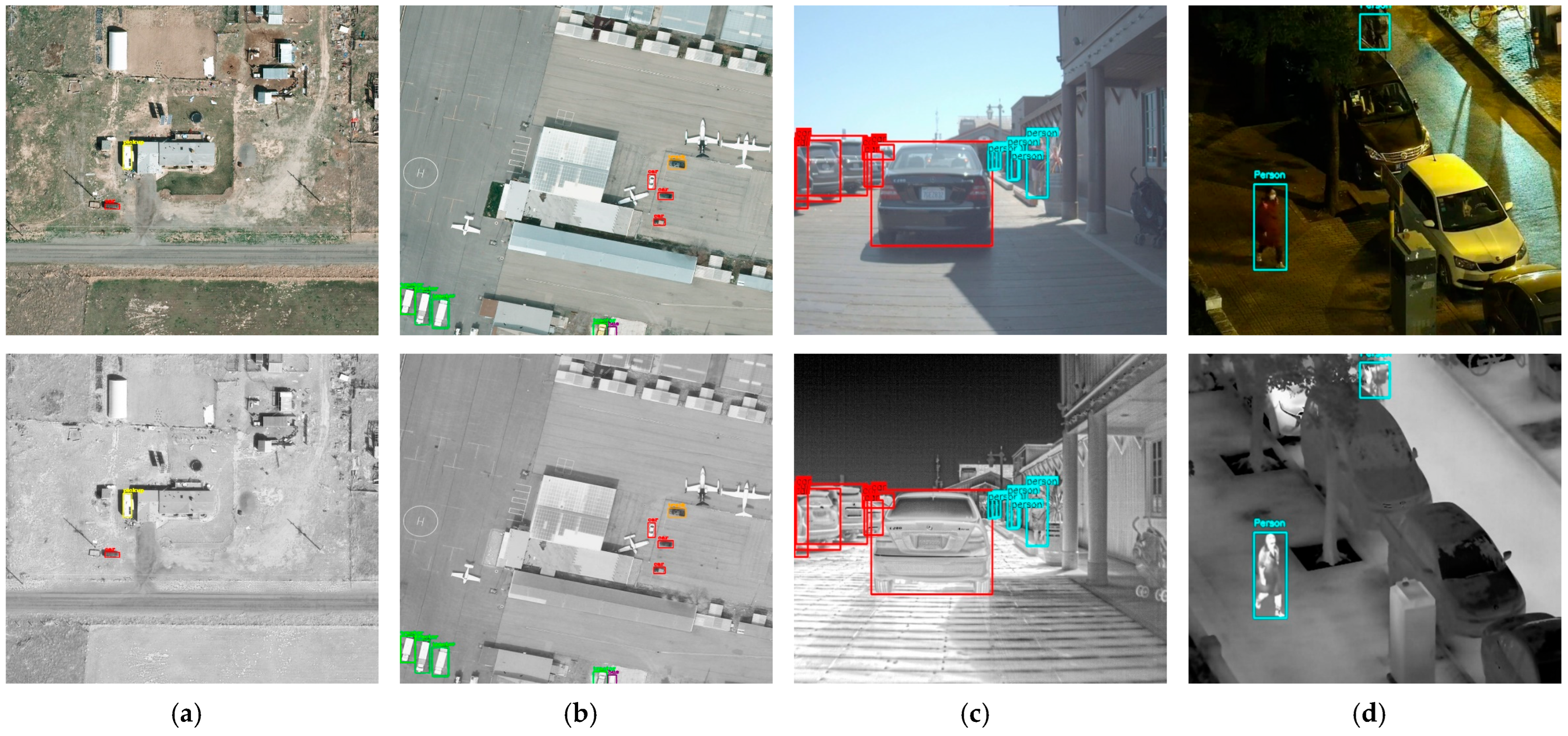
Figure 1.
Comparison of multispectral object detection advantages under different lighting conditions. The figure shows detection results for visible (top row) and infrared (bottom row) imaging in daytime (a–c) and nighttime (d) scenes. It clearly demonstrates that visible images (top row) provide richer color and texture information for better detection in daylight, while infrared images (bottom row) provide clearer object contours by capturing thermal radiation, showing significant advantages in low-light conditions. This complementarity proves the necessity of multispectral fusion for all-weather object detection, especially in complex and variable environmental conditions.
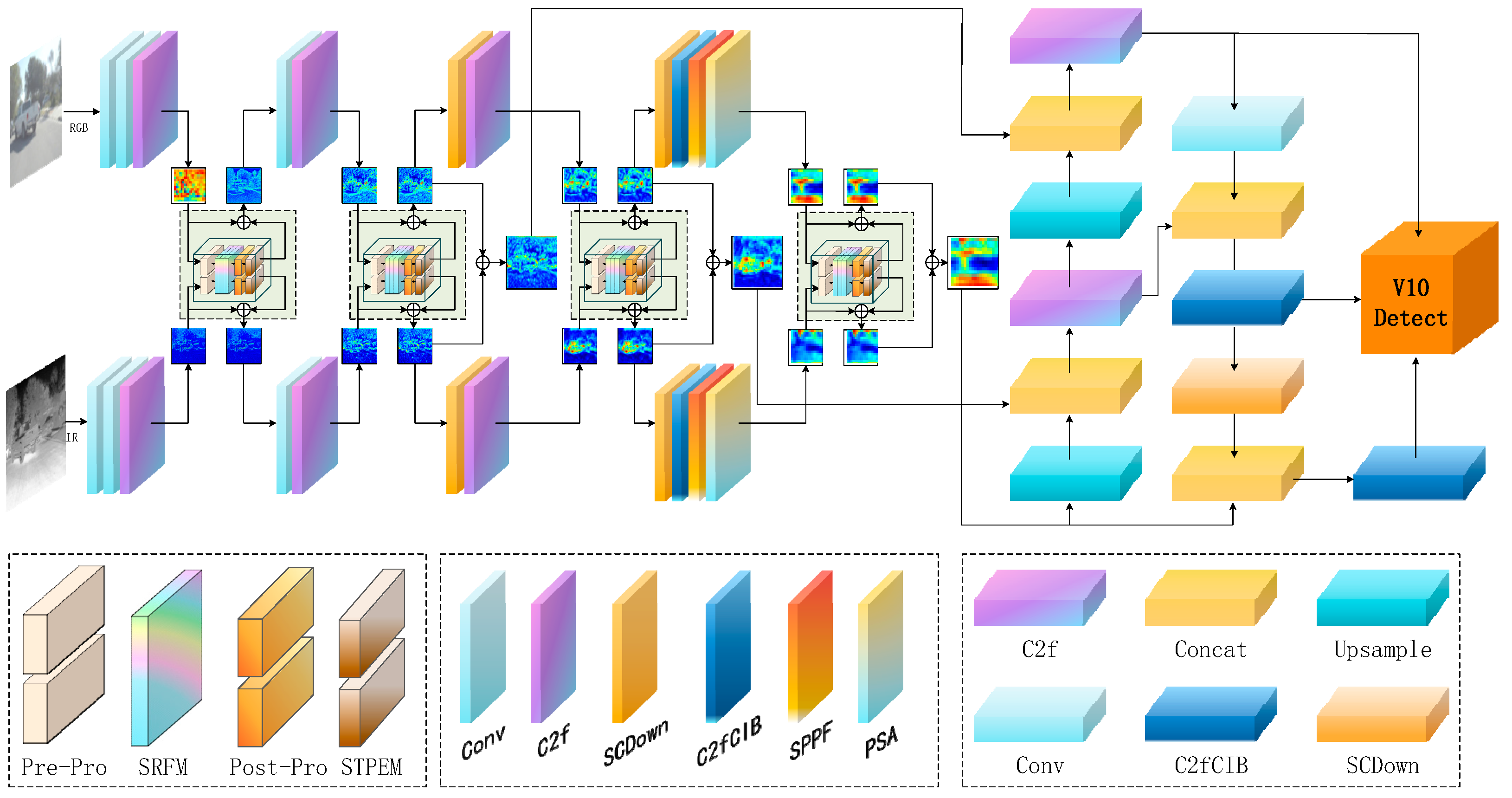
Figure 2.
Overall architecture of SDRFPT-Net (Spectral Dual-stream Recursive Fusion Perception Target Network). The architecture employs a dual-stream design with parallel processing paths for visible and infrared input images. The upper stream processes RGB features through C2f, C2f, SPPF, and C2f modules, while the lower stream handles IR features through identical but independently parameterized modules. Pre-Pro modules perform preprocessing including normalization and reshaping. The SRFM modules (marked in blue) conduct recursive fusion at multiple scales (P3/8, P4/16, P5/32). Post-Pro and STPEM modules enhance target perception before final feature aggregation through FPN and PAN structures. The network consists of three key innovative modules: Spectral Hierarchical Perception Architecture (SHPA) for extracting modality-specific features, Spectral Recursive Fusion Module (SRFM) for deep cross-modal feature interaction, and Spectral Target Perception Enhancement Module (STPEM) for enhancing target region representation and suppressing background interference. The feature pyramid and detection head (V10 Detect) enable multi-scale object detection.
![Remotesensing 17 02312 g002]()
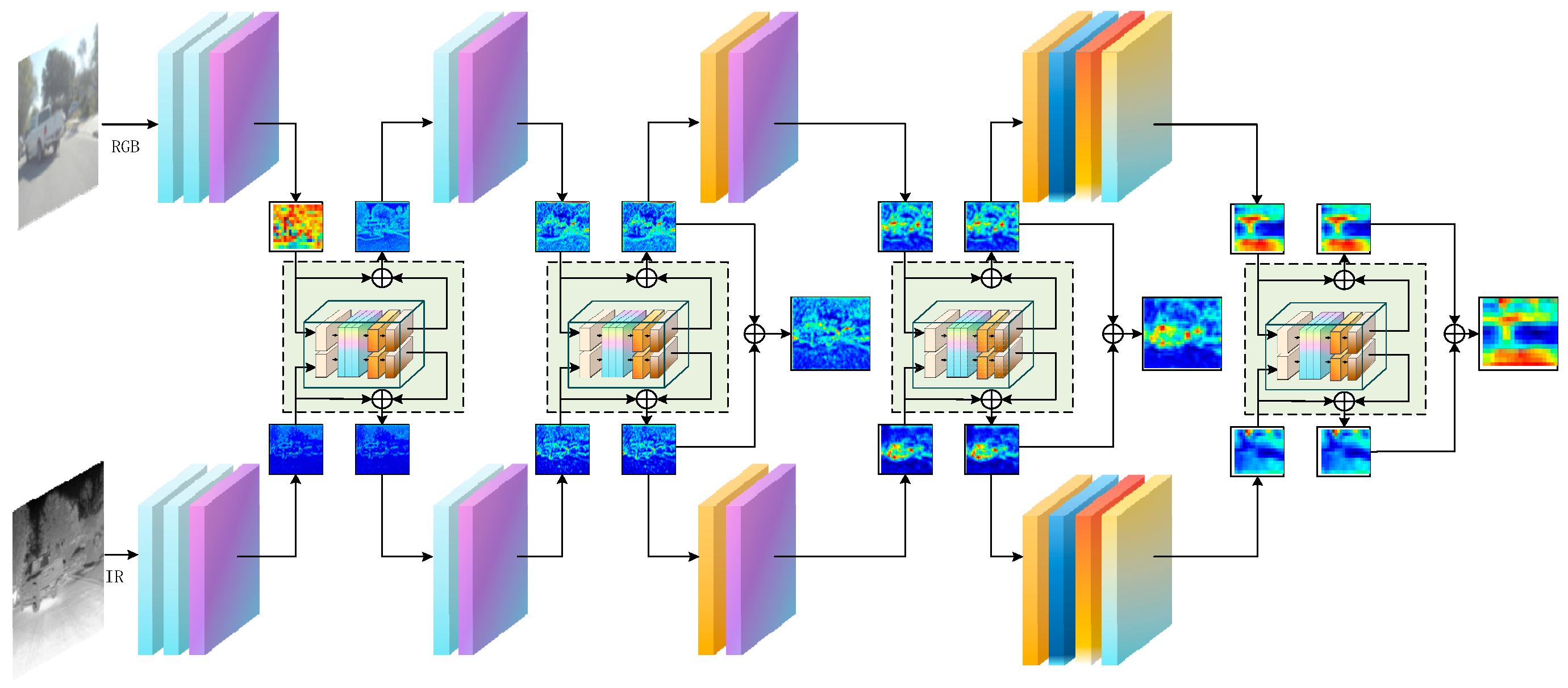
Figure 3.
Dual-stream separated spectral architecture design in SDRFPT-Net. The architecture expands a single feature extraction network into a dual-stream structure, where the upper stream processes visible spectral information, while the lower stream handles infrared spectral information. Although both processing paths share similar network structures, they employ independent parameter sets for optimization, allowing each stream to specifically learn the feature distribution and representation of its respective modality.
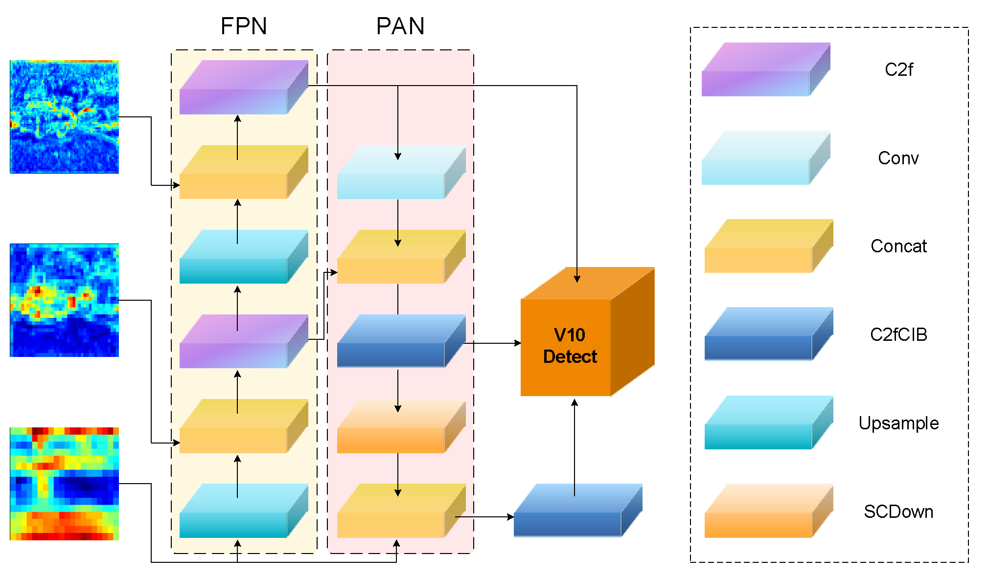
Figure 4.
Multi-scale fusion feature aggregation and detection process in SDRFPT-Net. The figure shows features from three different scales (P3, P4, P5) that already contain fused information from visible and infrared modalities. The middle section presents two complementary information flow networks: the Feature Pyramid Network (FPN), and Path Aggregation Network (PAN). The FPN process (light yellow background) follows Equation (8) where Pi = FPNi (Ffused), implementing a top-down pathway for semantic feature enhancement, while the PAN process (light pink background) follows Equation (9) where Mi represents the aggregated output through bottom-up feature integration. The right-hand side of the figure shows the network layer components including C2f modules for feature extraction, Conv layers for convolution operations, Concat for feature concatenation, C2fCIB for enhanced feature processing, Upsample for feature upsampling, and SCDown for spatial compression and downsampling. This bidirectional feature flow mechanism ensures that features at each scale incorporate both fine spatial localization information and rich semantic representation.
![Remotesensing 17 02312 g004]()
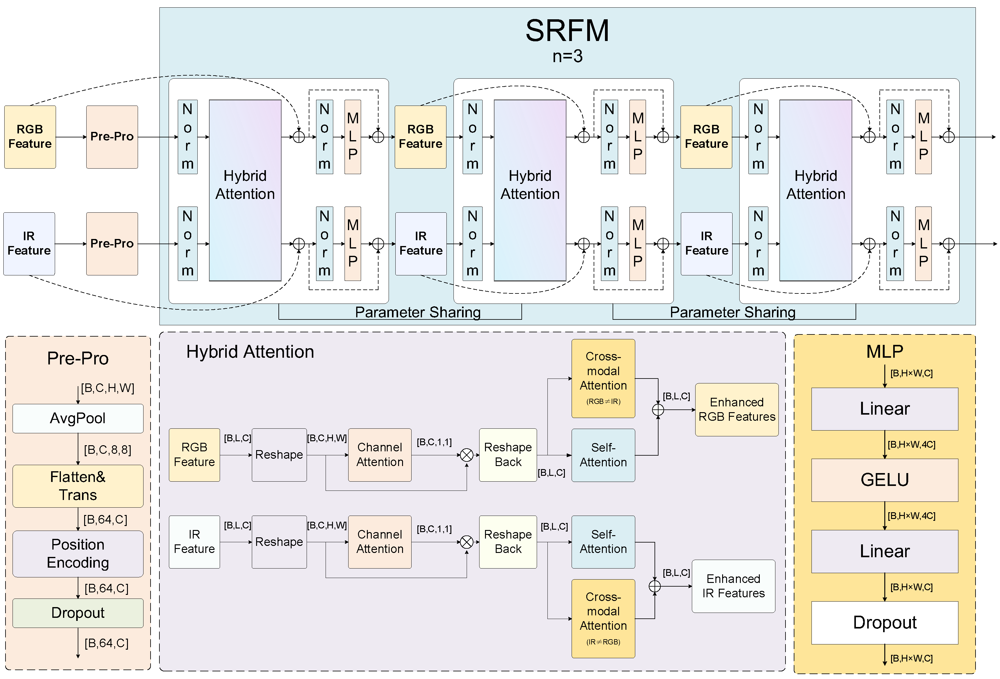
Figure 5.
Detailed architecture of the Spectral Recursive Fusion Module (SRFM). The framework is divided into two main parts: The upper light blue background area shows the overall recursive fusion process, labeled as ‘SRFM n = 3’, indicating a three-round recursive fusion strategy. This part receives RGB and IR dual-stream features from SHPA and processes them through three cascaded hybrid attention units with parameter sharing to improve computational efficiency. The lower part shows the detailed internal structure of the hybrid attention unit, including preprocessing components (Pre-Pro) such as AvgPool, Flatten, and Position Encoding; the hybrid attention mechanism implementation including Channel Attention, Self-Attention, and Cross-modal Attention; and the MLP module with Linear layers, GELU activation, and Dropout.
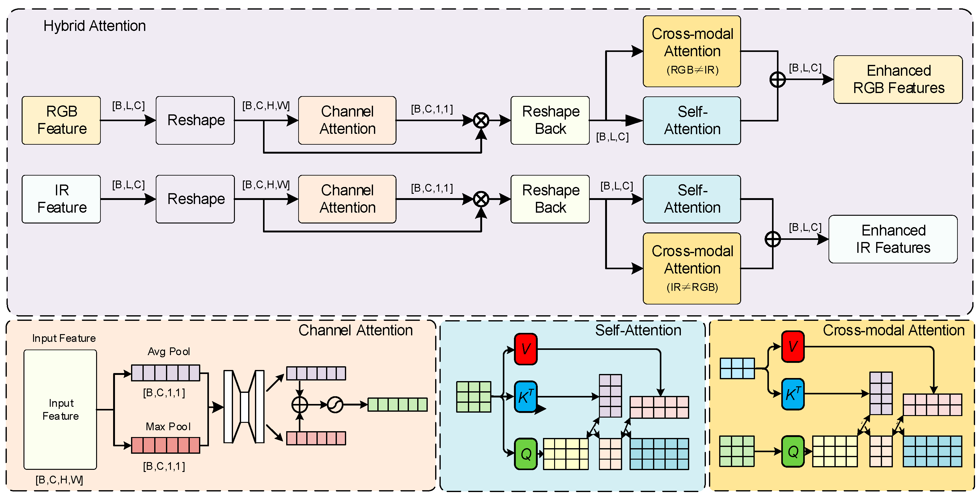
Figure 6.
Detailed structure of the hybrid attention mechanism in SDRFPT-Net. The mechanism integrates three complementary attention computation methods to achieve multi-dimensional feature enhancement. The upper part shows the overall processing flow: RGB and IR features first undergo reshaping and enter the Channel Attention module, which focuses on learning the importance weights of different feature channels. After reshaping back, the features simultaneously enter both the Self-Attention and Cross-modal Attention modules, capturing intra-modal spatial dependencies and inter-modal complementary information. The Cross-modal Attention modules implement the CrossAtt functions shown in Equations (11) and (12), where RGB features cross-attend to IR features and vice versa, as illustrated by the bidirectional connections between the RGB and IR processing streams in the lower part of the figure. Finally, the outputs from both attention modules are added to generate enhanced RGB and IR feature representations.
![Remotesensing 17 02312 g006]()
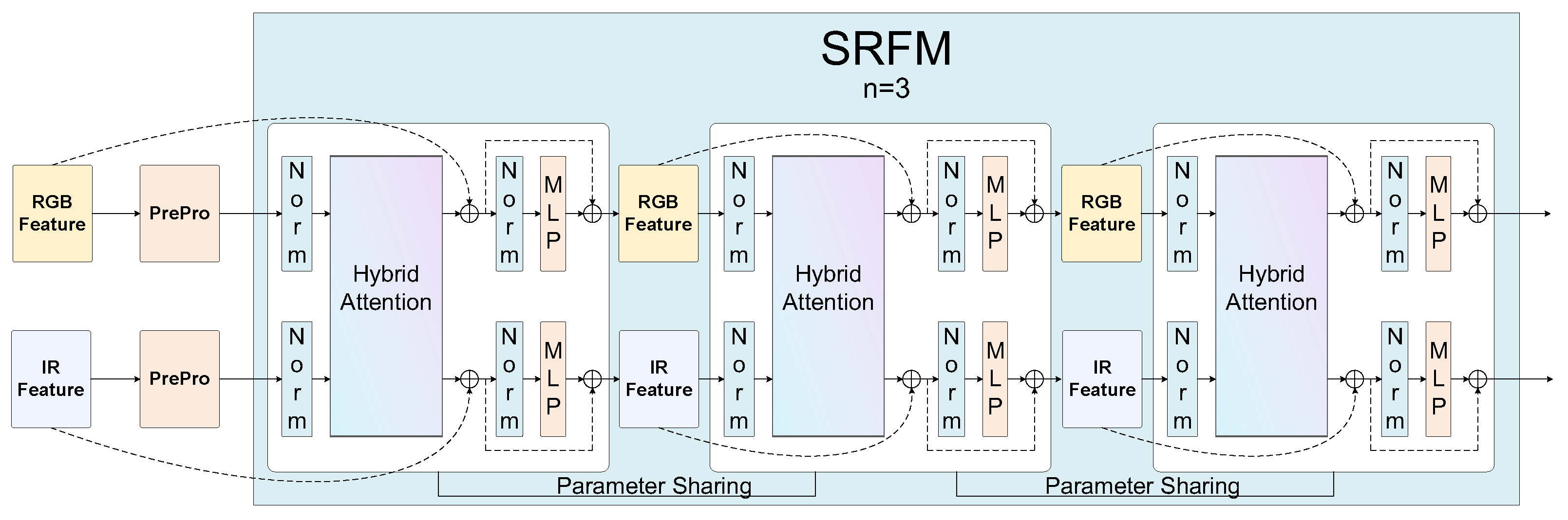
Figure 7.
Spectral recursive progressive fusion architecture in SDRFPT-Net. The light blue background area (labeled as ‘SRFM n = 3’) shows the parameter-sharing three-round recursive fusion process. The left side includes RGB and IR input features after preprocessing (Pre-Pro), which flow through three cascaded hybrid attention units. The key innovation is that these three processing units share the exact same parameter set (indicated by ‘Parameter Sharing’ connections), achieving deep recursive structure without increasing model complexity. Each processing unit contains normalization (Norm) components and MLP modules, forming a complete feature refinement path.
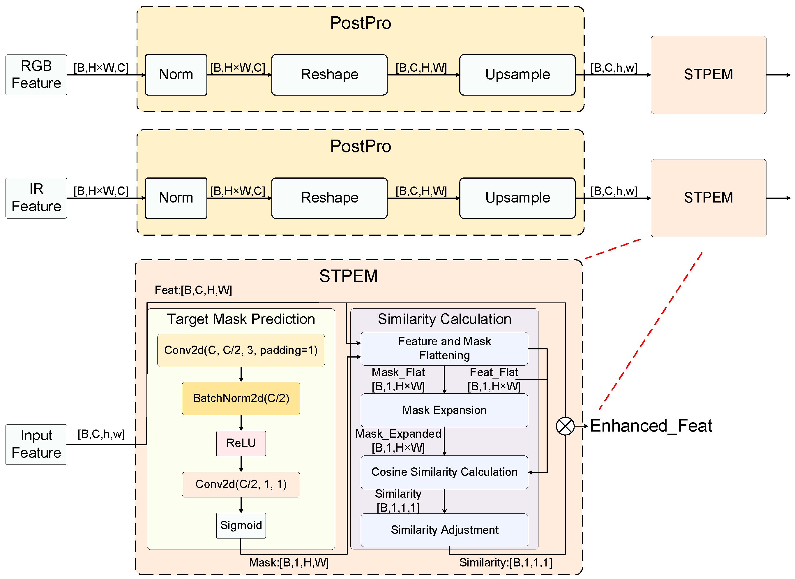
Figure 8.
Spectral Target Perception Enhancement Module (STPEM) structure and data flow. The module aims to enhance target region representation while suppressing background interference to improve detection accuracy. The figure is divided into three main parts: the upper and middle parts show parallel processing paths for features from RGB and IR modalities. Both feature paths first go through post-processing (Post-Pro) modules, including feature normalization, reshaping, and upsampling, before entering the STPEM module for enhancement processing.
Figure 9.
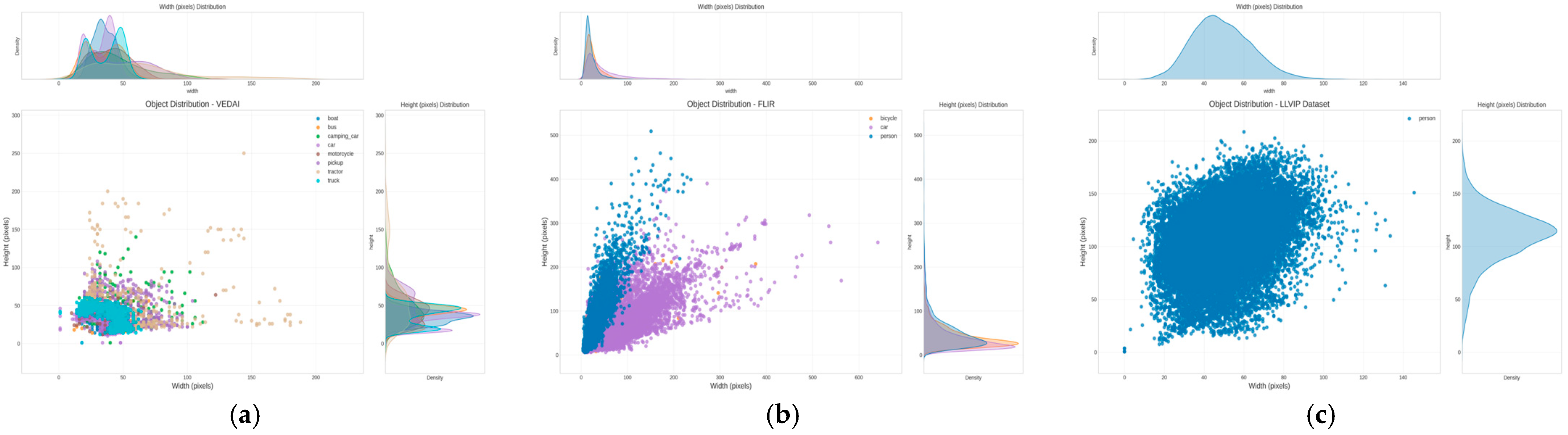
Object size distribution characteristics in multispectral detection datasets. (a) VEDAI dataset: The scatter plot shows 3700+ annotated vehicle targets across eight classes. Each point represents one object instance plotted by width (x-axis, 0–300 pixels) versus height (y-axis, 0–300 pixels). Color coding indicates vehicle types: boats (green), buses (red), camping cars (blue), cars (yellow), motorcycles (cyan), pickups (magenta), tractors (black), and trucks (orange). The main cluster centers around 20–100 pixel width and 10–100 pixel height, with tractors showing the largest height variance (up to 250 pixels). The marginal histograms display frequency distributions for width (top) and height (right). (b) FLIR-aligned dataset: Three object classes are color-coded as blue (person, 2845 instances), purple (car, 1674 instances), and orange (bicycle, 267 instances). Persons form a distinctive vertical cluster (narrow width 20–80 pixels, extended height 50–400 pixels), cars display a triangular distribution pattern reflecting viewing angle variations, and bicycles occupy an intermediate size range. (c) LLVIP dataset: Shows 16,836 pedestrian instances with highly concentrated circular clustering (width 20–80 pixels, height 40–150 pixels), indicating consistent target scales in nighttime surveillance scenarios. The tight clustering reflects controlled imaging conditions and uniform pedestrian detection ranges.
Figure 9.
Object size distribution characteristics in multispectral detection datasets. (a) VEDAI dataset: The scatter plot shows 3700+ annotated vehicle targets across eight classes. Each point represents one object instance plotted by width (x-axis, 0–300 pixels) versus height (y-axis, 0–300 pixels). Color coding indicates vehicle types: boats (green), buses (red), camping cars (blue), cars (yellow), motorcycles (cyan), pickups (magenta), tractors (black), and trucks (orange). The main cluster centers around 20–100 pixel width and 10–100 pixel height, with tractors showing the largest height variance (up to 250 pixels). The marginal histograms display frequency distributions for width (top) and height (right). (b) FLIR-aligned dataset: Three object classes are color-coded as blue (person, 2845 instances), purple (car, 1674 instances), and orange (bicycle, 267 instances). Persons form a distinctive vertical cluster (narrow width 20–80 pixels, extended height 50–400 pixels), cars display a triangular distribution pattern reflecting viewing angle variations, and bicycles occupy an intermediate size range. (c) LLVIP dataset: Shows 16,836 pedestrian instances with highly concentrated circular clustering (width 20–80 pixels, height 40–150 pixels), indicating consistent target scales in nighttime surveillance scenarios. The tight clustering reflects controlled imaging conditions and uniform pedestrian detection ranges.
![Remotesensing 17 02312 g009]()
Figure 10.
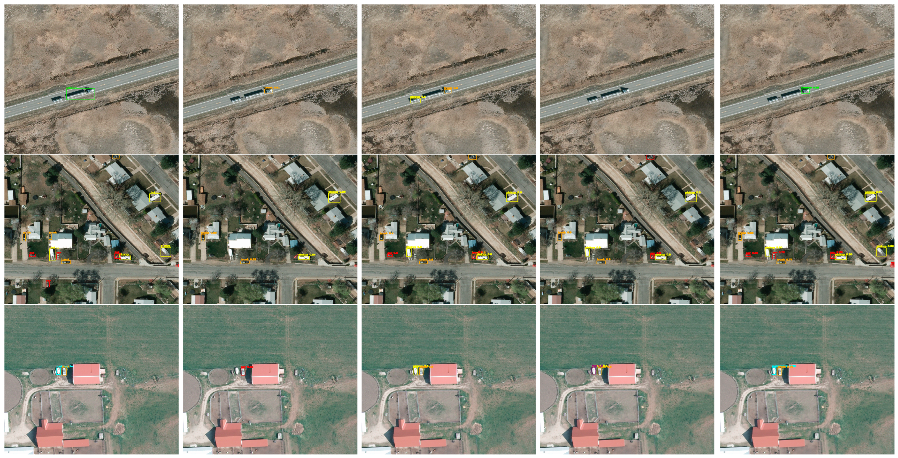
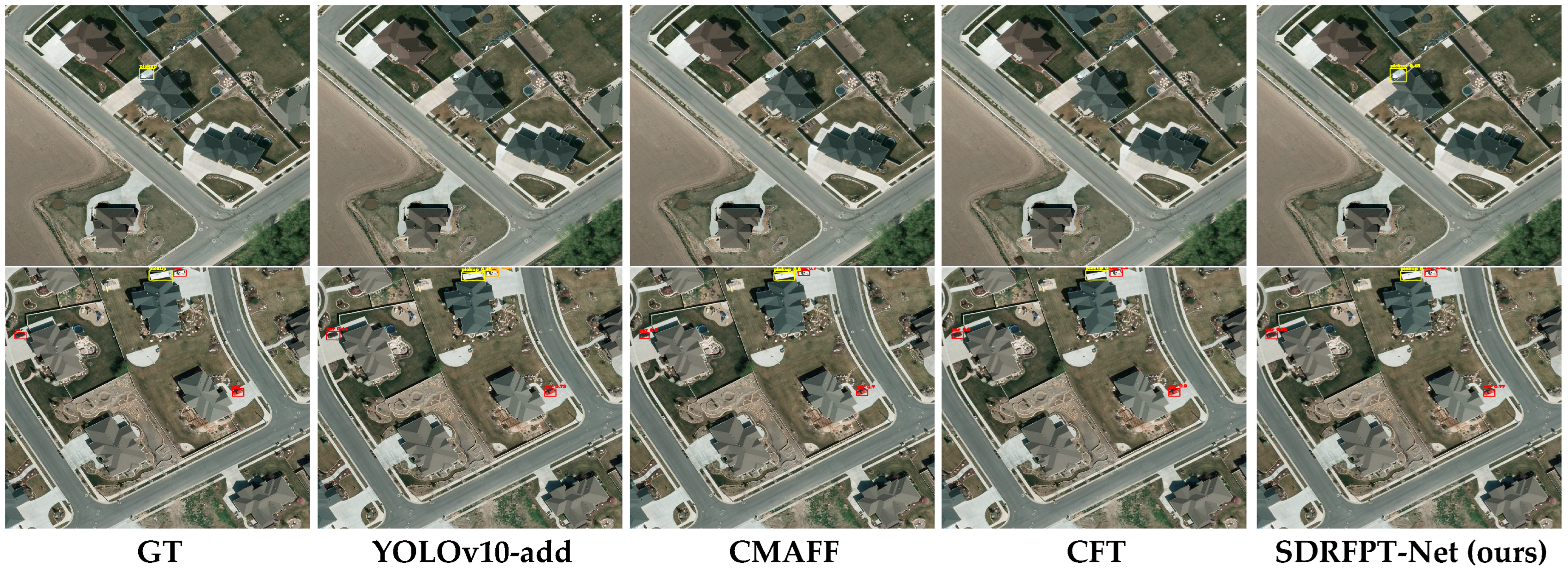
Comparison of detection performance for different multispectral object detection models on the VEDAI dataset. Images are organized by columns from left to right: Ground Truth (GT), YOLOv10-add, CMAFF, CFT, and our proposed SDRFPT-Net model. Each row displays typical remote sensing scenarios with different environmental conditions and object distributions, including roads, building clusters, and open areas, from an aerial perspective. The visualization results clearly demonstrate the advantages of SDRFPT-Net: under complex terrain textures and multi-scale remote sensing imaging conditions, SDRFPT-Net can accurately detect all targets with more precise bounding box localization. In contrast, other methods such as YOLOv10-add, CMAFF, and CFT exhibit certain limitations in small target detection and bounding box localization accuracy.
Figure 10.
Comparison of detection performance for different multispectral object detection models on the VEDAI dataset. Images are organized by columns from left to right: Ground Truth (GT), YOLOv10-add, CMAFF, CFT, and our proposed SDRFPT-Net model. Each row displays typical remote sensing scenarios with different environmental conditions and object distributions, including roads, building clusters, and open areas, from an aerial perspective. The visualization results clearly demonstrate the advantages of SDRFPT-Net: under complex terrain textures and multi-scale remote sensing imaging conditions, SDRFPT-Net can accurately detect all targets with more precise bounding box localization. In contrast, other methods such as YOLOv10-add, CMAFF, and CFT exhibit certain limitations in small target detection and bounding box localization accuracy.
Figure 11.
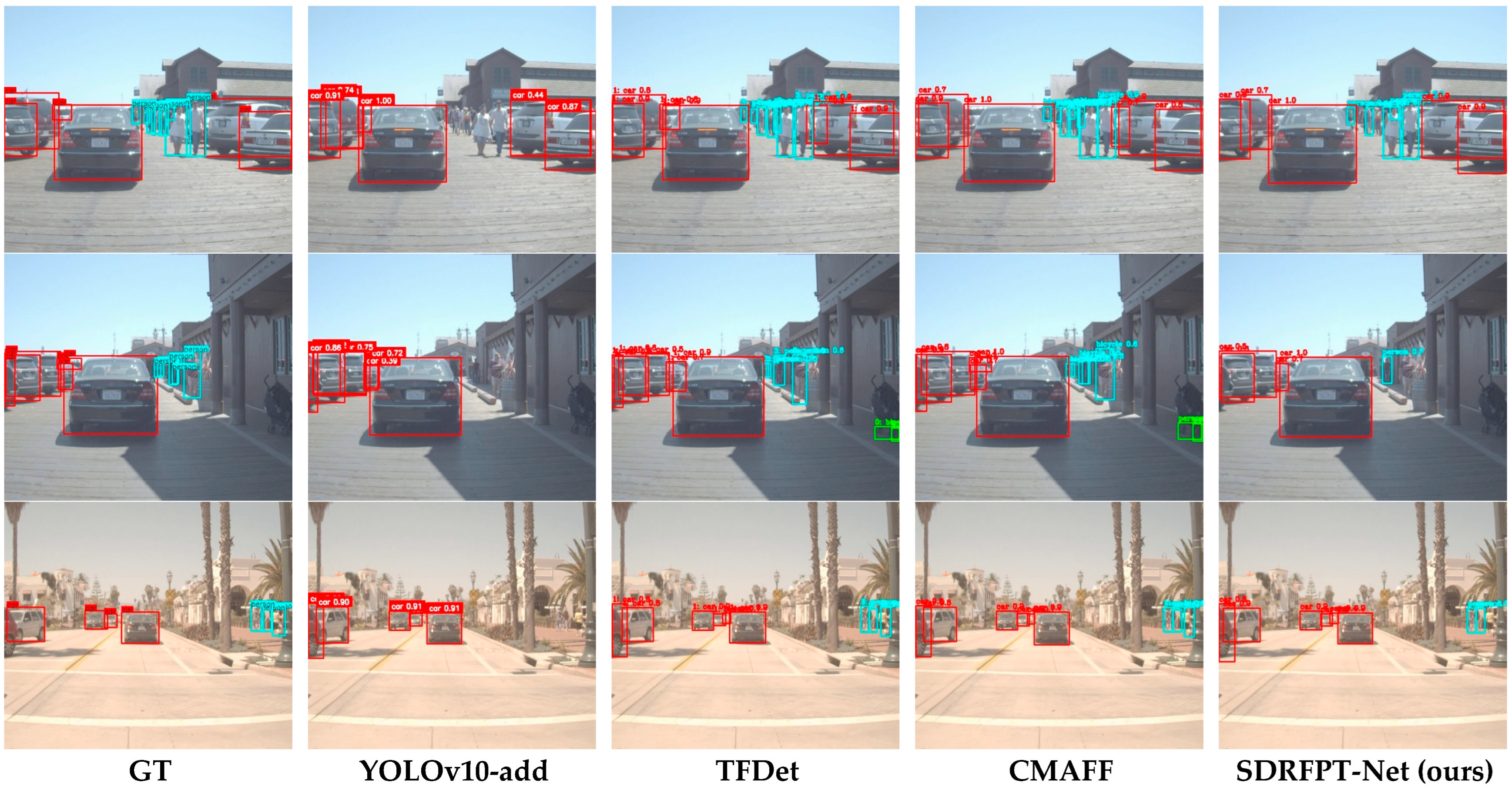
Comparison of detection performance for different multispectral object detection models on various scenarios in the FLIR-aligned dataset. Images are organized by columns from left to right: Ground Truth (GT), YOLOv10-add, TFDet, CMAFF, and our proposed SDRFPT-Net model. Each row shows typical scenarios with different environmental conditions and object distributions, including close-range vehicles, multiple roadway targets, parking areas, narrow streets, and open roads. The visualization results clearly demonstrate the advantages of SDRFPT-Net: In the first row’s close-range vehicle scene, SDRFPT-Net’s bounding boxes almost perfectly match GT. In the second row’s complex multi-target scene, it successfully detects all pedestrians and bicycles without obvious misses. In the third row’s parking lot scene, it accurately identifies multiple closely parked vehicles with precise bounding box localization.
Figure 11.
Comparison of detection performance for different multispectral object detection models on various scenarios in the FLIR-aligned dataset. Images are organized by columns from left to right: Ground Truth (GT), YOLOv10-add, TFDet, CMAFF, and our proposed SDRFPT-Net model. Each row shows typical scenarios with different environmental conditions and object distributions, including close-range vehicles, multiple roadway targets, parking areas, narrow streets, and open roads. The visualization results clearly demonstrate the advantages of SDRFPT-Net: In the first row’s close-range vehicle scene, SDRFPT-Net’s bounding boxes almost perfectly match GT. In the second row’s complex multi-target scene, it successfully detects all pedestrians and bicycles without obvious misses. In the third row’s parking lot scene, it accurately identifies multiple closely parked vehicles with precise bounding box localization.
Figure 12.
Comparison of pedestrian detection performance for different detection models on nighttime low-light scenes from the LLVIP dataset. Images are organized by columns from left to right: Ground Truth (GT), YOLOv10-add, TFDet, CMAFF, and our proposed SDRFPT-Net model. The rows display five typical nighttime scenes representing challenging situations with different lighting conditions, viewing angles, and target distances. In all low-light scenes, SDRFPT-Net demonstrates excellent pedestrian detection capability: The model accurately identifies distant pedestrians with precise bounding boxes in the first row’s street lighting scene, maintains stable detection performance despite strong light interference in the second and fourth rows, and successfully detects distant pedestrians that other methods tend to miss in the fifth row’s dark area.
Figure 13.
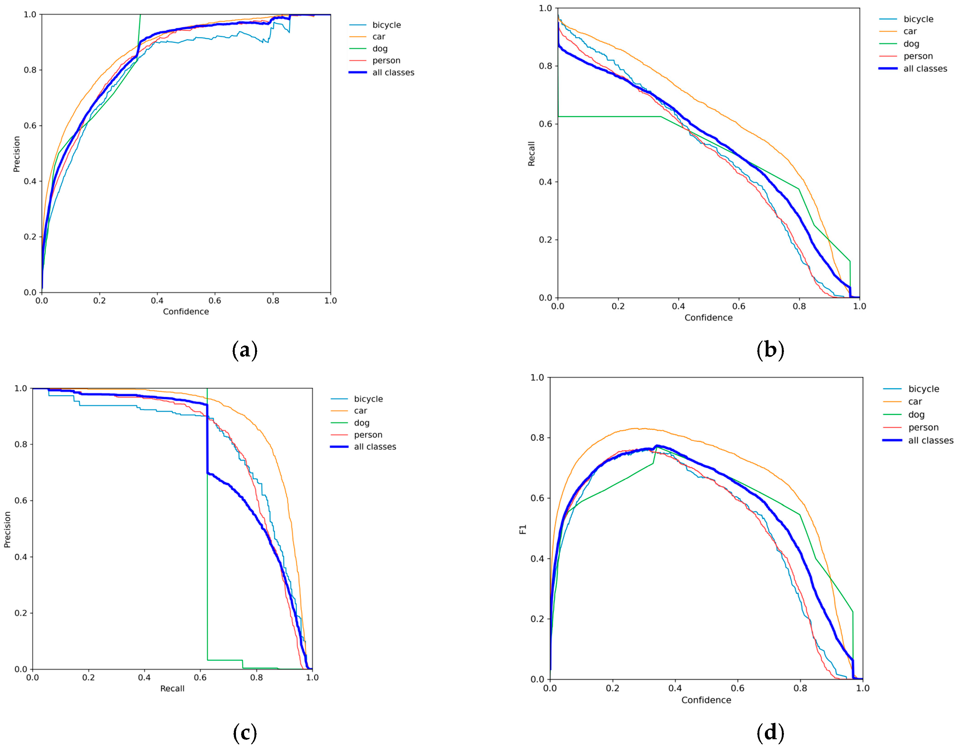
Learning curves of SDRFPT-Net on the FLIR-aligned dataset. (a) The precision–confidence curves show the variation in detection precision for each category under different confidence thresholds. (b) The recall–confidence curves demonstrate the trend in recall with confidence threshold changes. (c) The precision–recall curves reflect the performance trade-off at different operating points. (d) The F1–confidence curves comprehensively evaluate the overall detection performance of the model.
Figure 13.
Learning curves of SDRFPT-Net on the FLIR-aligned dataset. (a) The precision–confidence curves show the variation in detection precision for each category under different confidence thresholds. (b) The recall–confidence curves demonstrate the trend in recall with confidence threshold changes. (c) The precision–recall curves reflect the performance trade-off at different operating points. (d) The F1–confidence curves comprehensively evaluate the overall detection performance of the model.
Figure 14.
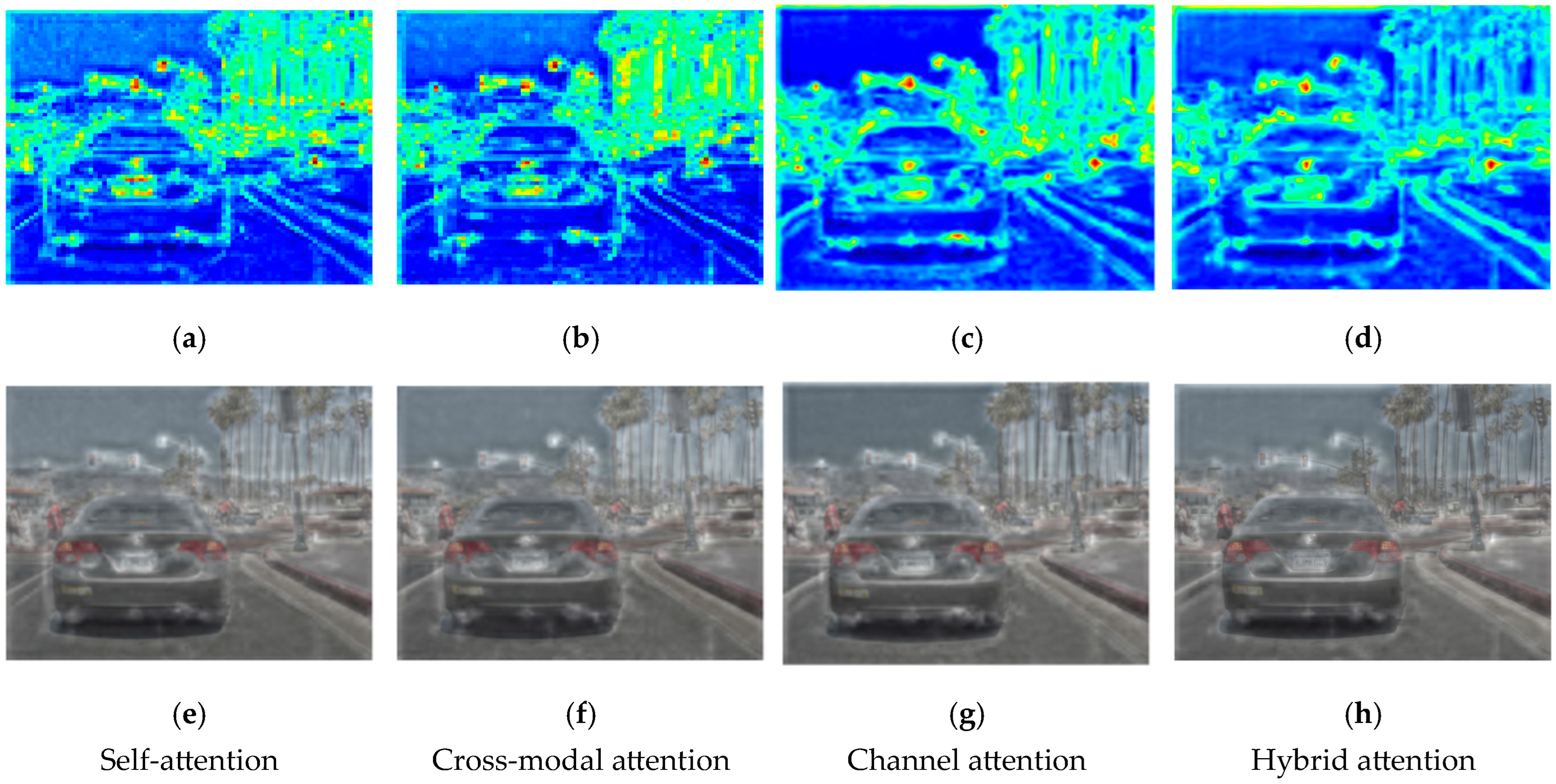
Comparative impact of different attention mechanisms on the P3 feature layer (high-resolution features) in SDRFPT-Net. The top row (a–d) presents feature activation maps, while the bottom row (e–h) shows the corresponding original image heatmap overlay effects, demonstrating the differences in feature attention patterns. Self-attention (a,e) focuses on target contours and edge information. Cross-modal attention (b,f) presents overall attention to target areas with complementary information from RGB and IR modalities. Channel attention (c,g) demonstrates selective enhancement of specific semantic information. Hybrid attention (d,h) combines the advantages of all three mechanisms for optimal feature representation.
Figure 14.
Comparative impact of different attention mechanisms on the P3 feature layer (high-resolution features) in SDRFPT-Net. The top row (a–d) presents feature activation maps, while the bottom row (e–h) shows the corresponding original image heatmap overlay effects, demonstrating the differences in feature attention patterns. Self-attention (a,e) focuses on target contours and edge information. Cross-modal attention (b,f) presents overall attention to target areas with complementary information from RGB and IR modalities. Channel attention (c,g) demonstrates selective enhancement of specific semantic information. Hybrid attention (d,h) combines the advantages of all three mechanisms for optimal feature representation.
Figure 15.
Representational differences between dual-attention mechanism combinations and the complete triple-attention mechanism on the P3 feature layer. The top row (a–d) shows feature activation maps, while the bottom row (e–h) shows original image heatmap overlay effects, revealing the complementarity and synergistic effects of different attention combinations. Self + Cross-modal attention (a,e) simultaneously possesses excellent boundary localization and target region representation; Self + Channel attention (b,f) enhances specific semantic features while preserving boundary information; Cross + Channel attention (c,g) enhances channel representation based on multi-modal fusion but lacks spatial context. Hybrid attention (d,h) achieves the most comprehensive and effective feature representation through synergistic integration of all three mechanisms.
Figure 16.
Comparison between simple addition fusion and innovative fusion strategies (SRFM + STPEM) on three feature scale layers. The upper row (a–c) presents traditional simple addition fusion at different scales: The P3/8 high-resolution layer (a) shows dispersed activation with insufficient target–background differentiation. The P4/16 medium-resolution layer (b) has some response to vehicle areas but with blurred boundaries. The P5/32 low-resolution layer (c) only has a rough response to the central vehicle. The lower row (d–f) shows feature maps of the innovative fusion strategy: The P3/8 layer (d) provides clearer vehicle contour representation with precise edge localization. The P4/16 layer (e) shows more concentrated target area activation. The P5/32 layer (f) preserves richer scene semantic information while enhancing central target representation.
Figure 17.
Impact of iteration counts (n = 1 to n = 5) in the recursive progressive fusion strategy on three feature scale layers of SDRFPT-Net. By comparing the evolution within the same row, changes in features with recursive depth can be observed. By comparing different rows, response characteristics at different scales can be understood. The P3 high-resolution layer (a–e) shows feature representation gradually evolving from initial dispersed response (n = 1) to more focused target contours (n = 2, 3), with clearer boundaries and stronger background suppression, but experiencing over-smoothing at n = 4, 5. The P4 medium-resolution layer (f–j) shows optimal target–background differentiation at n = 3, followed by feature response diffusion at n = 4, 5. The P5 low-resolution layer (k–o) presents the most significant changes, achieving highly structured representation at n = 3 that clearly distinguishes main scene elements, while showing obvious degradation at n = 4 and n = 5.
Table 1.
Performance comparison of SDRFPT-Net with state-of-the-art methods on the VEDAI dataset. The table presents precision (P), recall (R), mean average precision at IoU threshold of 0.5 (mAP50), and mean average precision across IoU thresholds from 0.5 to 0.95 (mAP50:95). V-I indicates the fusion of visible and infrared modalities. The best results are highlighted in bold.
| Methods | Modality | P | R | mAP50 | mAP50:95 |
|---|
| YOLOv5 | Visible | 0.704 | 0.604 | 0.675 | 0.398 |
| Infrared | 0.521 | 0.514 | 0.498 | 0.280 |
| YOLOv8 | Visible | 0.727 | 0.431 | 0.537 | 0.333 |
| Infrared | 0.520 | 0.523 | 0.494 | 0.291 |
| YOLOv10 | Visible | 0.610 | 0.523 | 0.587 | 0.329 |
| Infrared | 0.421 | 0.463 | 0.447 | 0.244 |
| DETR | Visible | 0.682 | 0.548 | 0.621 | 0.356 |
| Infrared | 0.547 | 0.489 | 0.532 | 0.298 |
| YOLOv10-add | V-I | 0.500 | 0.527 | 0.537 | 0.276 |
| CFT | V-I | 0.701 | 0.627 | 0.672 | 0.427 |
| CMAFF | V-I | 0.616 | 0.508 | 0.452 | 0.275 |
| SuperYOLO | V-I | 0.790 | 0.678 | 0.716 | 0.425 |
| SDRFPT-Net (ours) | V-I | 0.796 | 0.683 | 0.734 | 0.450 |
Table 2.
Performance comparison of SDRFPT-Net with state-of-the-art methods on the FLIR-aligned dataset. The table presents precision (P), recall (R), mean average precision at IoU threshold of 0.5 (mAP50), and mean average precision across IoU thresholds from 0.5 to 0.95 (mAP50:95). The best results are highlighted in bold.
| Methods | Modality | P | R | mAP50 | mAP50:95 |
|---|
| YOLOv5 | Visible | 0.531 | 0.395 | 0.441 | 0.202 |
| Infrared | 0.625 | 0.468 | 0.539 | 0.272 |
| YOLOv8 | Visible | 0.532 | 0.396 | 0.448 | 0.218 |
| Infrared | 0.559 | 0.514 | 0.549 | 0.288 |
| YOLOv10 | Visible | 0.727 | 0.538 | 0.620 | 0.305 |
| Infrared | 0.773 | 0.618 | 0.727 | 0.424 |
| DETR | Visible | 0.698 | 0.521 | 0.595 | 0.289 |
| Infrared | 0.741 | 0.592 | 0.681 | 0.378 |
| YOLOv10-add | V-I | 0.748 | 0.623 | 0.701 | 0.354 |
| CMA-Det | V-I | 0.812 | 0.468 | 0.518 | 0.237 |
| TFDet | V-I | 0.827 | 0.606 | 0.653 | 0.346 |
| CMAFF | V-I | 0.792 | 0.550 | 0.558 | 0.302 |
| BA-CAMF Net | V-I | 0.798 | 0.632 | 0.704 | 0.351 |
| SDRFPT-Net (ours) | V-I | 0.854 | 0.700 | 0.785 | 0.426 |
Table 3.
Performance comparison of SDRFPT-Net with state-of-the-art methods on the LLVIP dataset. The table presents precision (P), recall (R), mean average precision at IoU threshold of 0.5 (mAP50), and mean average precision across IoU thresholds from 0.5 to 0.95 (mAP50:95). V-I indicates the fusion of visible and infrared modalities. The best results are highlighted in bold.
| Methods | Modality | P | R | mAP50 | mAP50:95 |
|---|
| YOLOv5 | Visible | 0.906 | 0.820 | 0.895 | 0.504 |
| Infrared | 0.962 | 0.898 | 0.960 | 0.631 |
| YOLOv8 | Visible | 0.933 | 0.829 | 0.896 | 0.513 |
| Infrared | 0.956 | 0.901 | 0.961 | 0.645 |
| YOLOv10 | Visible | 0.914 | 0.833 | 0.892 | 0.512 |
| Infrared | 0.962 | 0.909 | 0.961 | 0.637 |
| DETR | Visible | 0.889 | 0.795 | 0.863 | 0.485 |
| Infrared | 0.948 | 0.885 | 0.934 | 0.598 |
| YOLOv10-add | V-I | 0.961 | 0.893 | 0.957 | 0.628 |
| TFDet | V-I | 0.960 | 0.896 | 0.960 | 0.594 |
| CMAFF | V-I | 0.958 | 0.899 | 0.915 | 0.574 |
| BA-CAMF Net | V-I | 0.866 | 0.828 | 0.887 | 0.511 |
| SDRFPT-Net (ours) | V-I | 0.963 | 0.911 | 0.963 | 0.706 |
Table 4.
Impact of different attention combinations on detection performance. The table compares the effects of Self Attention, Cross-modal Attention, and Channel Attention in various combinations. The best results are highlighted in bold.
Table 4.
Impact of different attention combinations on detection performance. The table compares the effects of Self Attention, Cross-modal Attention, and Channel Attention in various combinations. The best results are highlighted in bold.
| ID | SHPA | SRFM | STPEM | mAP50 | mAP50:95 |
|---|
| A1 | ✔ | | | 0.701 | 0.354 |
| A2 | ✔ | ✔ | | 0.775 | 0.373 |
| A3 | ✔ | ✔ | ✔ | 0.785 | 0.426 |
Table 5.
Impact of different attention combinations on detection performance. The table compares the effects of self-attention, cross-modal attention, and channel attention in various combinations. The best results are highlighted in bold.
Table 5.
Impact of different attention combinations on detection performance. The table compares the effects of self-attention, cross-modal attention, and channel attention in various combinations. The best results are highlighted in bold.
| ID | Self-Attention | Cross-Attention | Channel-Attention | mAP50 | mAP50:95 |
|---|
| B1 | ✔ | | | 0.776 | 0.408 |
| B2 | | ✔ | | 0.749 | 0.372 |
| B3 | | | ✔ | 0.730 | 0.384 |
| B4 | ✔ | ✔ | | 0.774 | 0.424 |
| B5 | ✔ | | ✔ | 0.763 | 0.409 |
| B6 | | ✔ | ✔ | 0.729 | 0.362 |
| B7 | ✔ | ✔ | ✔ | 0.785 | 0.426 |
Table 6.
Ablation experiments on fusion positions. The table shows the impact of applying advanced fusion modules at different feature scales. P3/8, P4/16, and P5/32 represent feature maps at different scales, with numbers indicating the downsampling factor relative to the input image. The best results are highlighted in bold.
| ID | P3/8 | P4/16 | P5/32 | mAP50 | mAP50:95 |
|---|
| C1 | Add | Add | Add | 0.701 | 0.354 |
| C2 | SRFM + STPEM | Add | Add | 0.769 | 0.404 |
| C3 | SRFM + STPEM | SRFM + STPEM | Add | 0.776 | 0.410 |
| C4 | SRFM + STPEM | SRFM + STPEM | SRFM + STPEM | 0.785 | 0.426 |
Table 7.
Impact of different iteration counts of the recursive progressive fusion strategy on model detection performance. The experiment compares performance with recursive depths from 1 to 5 iterations (D1–D5), evaluating detection accuracy using mAP50 and mAP50:95 metrics. The best results are highlighted in bold.
| ID | Times | mAP50 | mAP50:95 |
|---|
| D1 | 1 | 0.769 | 0.395 |
| D2 | 2 | 0.783 | 0.418 |
| D3 | 3 | 0.785 | 0.426 |
| D4 | 4 | 0.783 | 0.400 |
| D5 | 5 | 0.761 | 0.417 |


