Abstract
There is a common need for optical sequence images with high spatiotemporal resolution. As a solution, Synthetic Aperture Radar (SAR)-to-optical translation tends to bring high temporal continuity of optical images and low interpretation difficulty of SAR images. Existing studies have been focused on converting a single SAR image into a single optical image, failing to utilize the advantages of repeated observations from SAR satellites. To make full use of periodic SAR images, it is proposed to investigate the sequential SAR-to-optical translation, which represents the first effort in this topic. To achieve this, a model based on a diffusion framework has been constructed, with twelve Transformer blocks utilized to effectively capture spatial and temporal features alternatively. A variational autoencoder is employed to encode and decode images, enabling the diffusion model to learn the distribution of features within optical image sequences. A conditional branch is specifically designed for SAR sequences to facilitate feature extraction. Additionally, the capture time is encoded and embedded into the Transformers. Two sequence datasets for the sequence translation task were created, comprising Sentinel-1 Ground Range Detected data and Sentinel-2 red/green/blue data. Our method was tested on new datasets and compared with three state-of-the-art single translation methods. Quantitative and qualitative comparisons validate the effectiveness of the proposed method in maintaining radiometric and spectral consistency.
1. Introduction
Sequential optical satellite images provide valuable observations of temporal and spatial changes for large-scale ground surveys, making them essential data sources for monitoring urban development, disasters, agriculture, and more. However, the availability of optical data is often limited due to its high susceptibility to weather conditions. Spatiotemporal fusion [1] and spatiotemporal-spectral fusion [2] can partially mitigate the impact of adverse weather by predicting missing images based on available optical data. Nevertheless, obtaining low-resolution reference optical images during prolonged rainy seasons remains difficult. In contrast, synthetic aperture radar (SAR) imaging, which utilizes microwaves to penetrate clouds, facilitates all-weather monitoring and significantly broadens the scope of remote sensing. Since SAR images are not easily interpreted, converting them into optical images can enhance usability for downstream applications. Additionally, synthesized optical images can be employed to restore optical images that are partially obscured by clouds or haze.
Solutions have emerged for one-to-one image translation from SAR images to optical images as a conditional image generation problem. The Generative Adversarial Network (GAN) framework is commonly used in these works [3,4,5,6,7], where the generators use the encoder–decoder framework. Convolutional neural networks (CNNs) were used for feature extraction, recombination, and deconvolution, and the discriminator improves the training quality of the generator. Besides GAN and CNNs, some works utilized visual Transformer and diffusion models [8], where attention mechanisms and data distribution learning are utilized separately.
Sequential SAR-to-optical translation holds promise due to the steady availability of repeated SAR observations, enabling temporal understanding of land covers. To leverage temporal information, methods such as Gaussian process regression [9] and deep learning-based approaches like recurrent neural networks (RNNs) [10,11] or Transformers [12] have been explored. Unfortunately, these algorithms targeted the synthesis of time series normalized difference vegetation index (NDVI) and cannot be used for multi-channel image generation.
In summary, there is currently no research demonstrating the feasibility of translating a SAR image sequence into an optical image sequence. The studies mentioned either performed single translations or achieved sequence translation from SAR to NDVI. To our knowledge, Peng et al. [13] conducted the only sequence translation from SAR to optical images, which necessitates auxiliary optical images as references and is essentially a fusion task. Clearly, direct translation from a SAR sequence to an optical sequence is challenging, as it involves modeling spatial, temporal, and spectral features simultaneously. Additionally, there is a significant lack of training data.
Multi-temporal SAR-to-optical image translation has potential of enhancing the generation quality, as it harnesses the sequential properties inherent in both SAR and optical imagery. SAR images record microwave backscatter coefficients. For land covers with unchanged structures, the SAR intensity is highly correlated with atmospheric water vapor content. This water vapor content is determined by atmospheric temperature and pressure, exhibits seasonal cycles, and fluctuates with meteorological conditions. Sequential SAR imagery captures the overarching trends of seasonal changes while also dynamically resolving short-term meteorological variations. These identified trends inform the decoder to generate optical images corresponding to specific seasons and weather conditions, thus enhancing the quality of the generated output. On the contrary, a single image cannot capture climactic dynamics nor reflect seasonal trends.
This work aims to translate sequential SAR images into sequential optical images. Our method takes multiple consecutive SAR images as input and produces temporally aligned optical images. The model employs a diffusion framework to learn the data distribution of optical images. A transformer architecture is utilized to model the temporal and spatial relationships between image patches. The process is conducted in a latent space using a variational autoencoder (VAE) to optimize memory usage. A conditional branch is designed to encode sequential SAR images, facilitating the synchronization of features between SAR and optical images. Additionally, the model incorporates the capture time of SAR images to enhance the generation of targets. To the best of our knowledge, this work represents the first sequential SAR-to-optical image translation method that does not rely on optical images. From the perspective of satellite observation, acquiring SAR sequences is nearly as straightforward as obtaining a single SAR image; thus, the practical value of this work remains significant despite the use of multiple SAR images.
To achieve this goal, sequential SAR–optical datasets have been constructed for the first time. The SAR images are sourced from Sentinel-1, while the optical images are obtained from Sentinel-2. The scenes are located in Australia and France. Therefore, we have two datasets which are named SeqSen12-FCA and SeqSen12-Paris, respectively. The sequences cover a period of up to one year. Our dataset can also be utilized for single SAR-to-optical image translation, which will be tested in this study.
The contributions of this work are summarized below.
- (1)
- This is the first study to generate multi-temporal optical images from a sequence of SAR images.
- (2)
- It created the first dataset for the conversion between sequential SAR images and sequential optical images.
- (3)
- It proposes a conditional diffusion model to address the challenge of sequential SAR-to-optical generation.
The rest of the paper is organized as follows. Section 2 introduces related works and the principle of the conditional diffusion model. Section 3 presents the proposed methodology. Section 4 presents the experimental plans and Section 5 provides experimental results, comparing different state-of-the-art methods with the proposed method. Section 6 discusses the potential of better performance. Section 7 draws conclusions based on the findings.
2. Related Work
This section gives a survey about recent progress in SAR-to-optical image translation, with a specific emphasis on the sequence translation technologies. For single translation, it discusses a range of GAN-based, Transformer-based, and diffusion-based methods. For sequence translation, RNN and Transformer are mentioned. Furthermore, the review delves into conditional diffusion models, which will be used in the next section for hybrid modeling.
2.1. Single SAR-to-Optical Translation
In recent years, some studies have suggested supervised SAR-to-optical image translation. These studies understood SAR images as ordinary images, addressed the translation as a style transfer issues and solved it with the encoder–decoder framework. The network structures, loss functions, and training strategies are deliberately designed in these work.
Most studies use the Generative Adversarial Network (GAN) framework to constrain the spectral accuracy of generated optical images. Wang et al. [4] proposed a bidirectional consistent adversarial network to synthesize optical images from input SAR images. Fu et al. [5] proposed a cascaded residual adversarial network for SAR to optical image conversion, which introduces cascaded residual connections and GAN loss. Tan et al. [14] designed two GAN models, one responsible for denoising SAR images and the other for coloring SAR images. Zhang et al. [15] introduced gradient information for SAR images and texture information such as contrast, uniformity, and correlation based on a gray level co-occurrence matrix into the generator to improve structural similarity. Guo et al. [16] proposed an edge preserving constraint for SAR to optical image translation, which enhances the structure of the translated image using the edge information of SAR images. Yang et al. [17] utilized multi-scale receptive fields and chromatic aberration loss to improve its translation ability. Li et al. [18] proposed a multi-scale generative adversarial network based on wavelet feature learning. Wei et al. [19] proposed a GAN that combines cross fusion inference and wavelet decomposition to preserve image structural details and enhance high-frequency band information.
The latest modeling techniques for translation include vision Transformer, diffusion models, and physics-guided explainable models. Wang et al. [6] proposed a hybrid GAN network that combines CNN and visual Transformer. Kong et al. [20] proposed an encoder–decoder structure generator based on the SWIN Transformer. Recently, Bai et al. [8] proposed a conditional diffusion model for the conversion of SAR to optical images. This model is based on the diffusion process and utilizes SAR images as constraints to convert Gaussian noise into real optical images. The diffusion-based generation model outperforms current GAN based models in generating optical images. Other applications of the diffusion model in SAR-to-optical image translation were found in [21,22]. As for the interpretable model, Zhang et al. [23] designed a third-order finite difference residual block in light of thermodynamics to efficiently extract inter-domain invariant features, and Zhang et al. [24] proposed a neural partial differential Equation (Taylor central difference)-based residual block to build the translation network.
2.2. Sequence Translation from SAR to NDVI
The reconstruction from time series to time series is traditionally understood as a time dimension interpolation problem, and the main sequence generation methods include local interpolation, global interpolation, Gaussian process regression, and so on. The local interpolation method uses a time series based on sliding time windows to infer the temporal changes in optical remote sensing images. Common methods include cubic spline interpolation, adaptive regression filtering, and Savitzky–Golay filtering algorithm. Global interpolation methods recover lost information by fitting data to pre-defined functions, including Whittaker smoothing, asymmetric Gaussian fitting, and harmonic analysis based on Fourier transform. Gaussian process regression is a supervised learning method that can be used to learn the interrelationships between multiple datasets [9].
Recently, deep learning-based sequence generation methods have gradually been used for the reconstruction of SAR sequence data to optical remote sensing sequence data. Zhao et al. [10] extended the traditional CNN-RNN model and proposed a deep learning network based on context sequences from multiple CNN sequences to RNN sequences. The network first uses multiple CNNs to extract feature information from SAR data, and it then uses RNNs to establish the connection between SAR sequence data and optical remote sensing sequence data. Li et al. [12] proposed an end-to-end spatiotemporal fusion method based on Transformer, which collaborated SAR and optical time series to reconstruct optical remote sensing sequences of cloudy areas. Roßberg and Schmitt [11] proposed a RNN model based on a Gated Recurrent Unit (GRU), which is suitable for processing variable sequence length sequence data and can effectively handle missing optical remote sensing data.
The generation of SAR sequences to optical sequences is expected to solve the issue of temporal resolution caused by weather factors, but the related research focused on the generation of NDVI sequences from SAR sequences. Apparently, the image generation is far more difficult than the prediction of NDVI. Therefore, the translation from SAR image sequences to optical image sequences remains an untouched issue.
2.3. Conditional Diffusion Model in the Latent Space
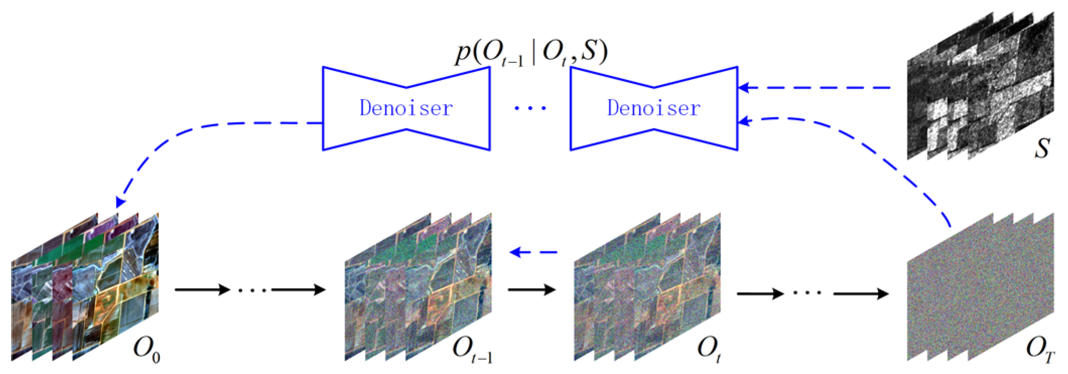
As shown in Figure 1, the conditional diffusion model in the latent space learns the distribution of features extracted from images using an encoder. It consists of a forward process and a backward process. In the forward process, random Gaussian noise is gradually added to the reference optical features to generate a noisy optical feature map . This can be denoted as
where and increases gradually from 0.0001 to 0.02 with the time step t .
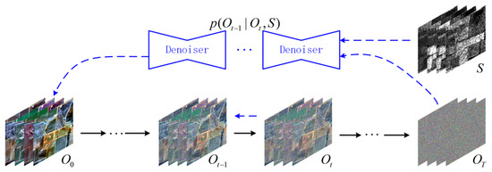
Figure 1.
Flowchart of the conditional diffusion model in the latent space.
By applying a reparameterization technique, the noisy feature can be represented as,
where .
The backward process involves training the conditional diffusion model to reverse the noise degradation introduced during the forward process, denoted as,
where S denotes the conditional SAR features that is concatenated with the noisy optical feature during model training and fed into the model.
The training of the model is constrained by the mean squared error (MSE) between the noise Z predicted by the network and the noise added during the forward process. To achieve accelerated sampling, a deterministic accelerated sampling strategy proposed in [25] is suggested. The sampling of the diffusion model is represented as
3. Methodology
This section describes the proposed method, which employs a diffusion framework to learn data distribution in latent space. The noise estimator within the diffusion model is implemented using cascaded Transformers. An encoding branch is specifically designed for sequential SAR images to extract features, which are then integrated into the noise estimator as a conditioning factor.
3.1. Framework: Latent Diffusion Model (LDM)
In translating SAR sequence into optical sequence, spatial and temporal relationships need to be modeled simultaneously. This article uses a latent diffusion model (LDM) to translate sequential SAR images into sequential optical images. LDM is a diffusion model that performs diffusion in the latent space which was used in stable diffusion [26]. For a given training dataset, LDM uses a pre-trained variational auto-encoder (VAE) to compress the data into a low-dimensional feature space, and then learns the distribution of features through forward and backward diffusion. The workflow of LDM is shown in Figure 1. Instead of using the CNN-based UNet model as the noise estimator [27], this work uses Transformer to simultaneously model spatial and temporal features. The network framework is similar to the latent diffusion transformer (Latte) model [28], but our model is more complicated as it has conditions and diverse inputs and outputs to adapt to the conversion from SAR to optical images. The VAE is critical as it reduces the huge memory demand of the diffusion process learning the distribution of a sequence.
3.2. Network Structures
Each step of forward diffusion is performed by adding noise to features of a clean image and training a denoiser to estimate the distribution of noise from the input noisy data, whereas the backward diffusion infers the clean image features with the trained denoiser. The core network of the noise estimator is designed using a Transformer-based conditional diffusion model. It models in both spatial and temporal dimensions to predict the injected noise. A conditional branch is designed to extracts spatial and temporal features from the referenced SAR sequence.
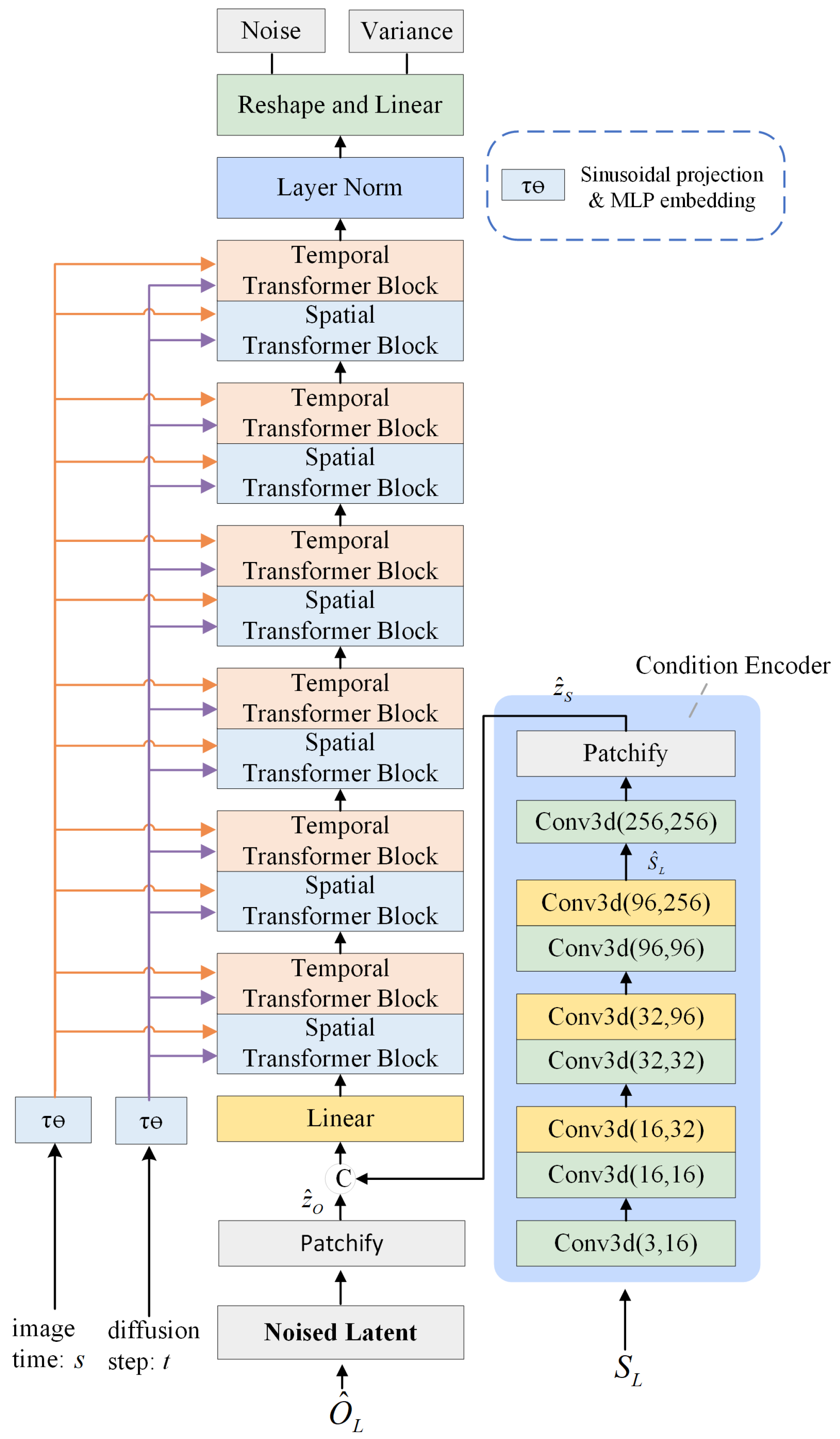
The structure is shown in Figure 2, which consists of a Transformer-based backbone and a condition branch. The backbone network consists of six spatial blocks and six temporal blocks alternating with each other to predict the new spatial and temporal features after injecting the SAR sequence features. The condition branch extracts multi-scale features of the reference SAR sequence by cascading five 3-dimensional (3D) convolutions and three downsampled 3D convolutions. Finally, the predicted mean values and variances of the noise are output through a linear layer, which are fed to Equation (4) to predict optical images.
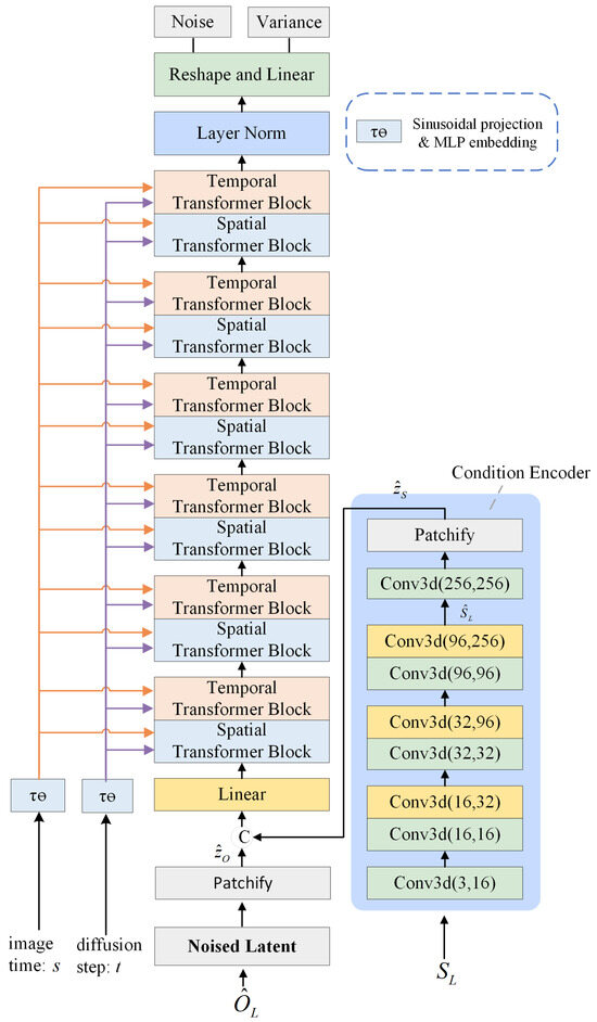
Figure 2.
Network structure. (The © symbol denotes the concatenation of raw images or feature maps).
3.2.1. Spatial Transformer and Temporal Transformer
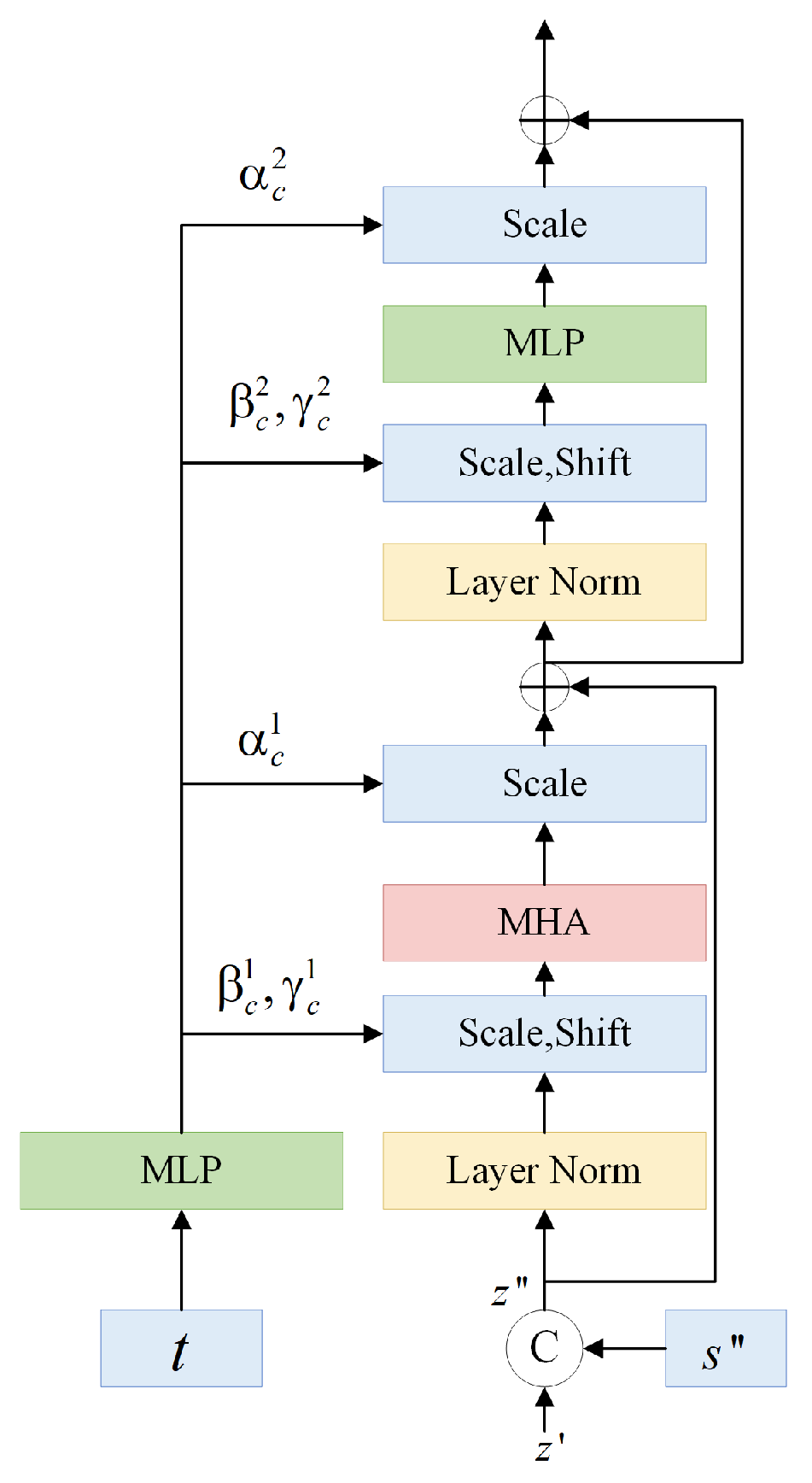
To predict the noise, the image features needed to be finely modeled after they are extracted from the VAE or the SAR encoder. Specifically, the feature patches are modeled in spatial Transformer blocks and temporal Transformer blocks, respectively. In our model, spatial features and temporal features are treated in the same way, while the only difference being the form in which the data are arranged. The structure of a spatial block or a temporal block is the same as that of a regular transformer block, consisting of a multi-head attention (MHA) block and a multi-layer perception (MLP) layer, as shown in Figure 3.
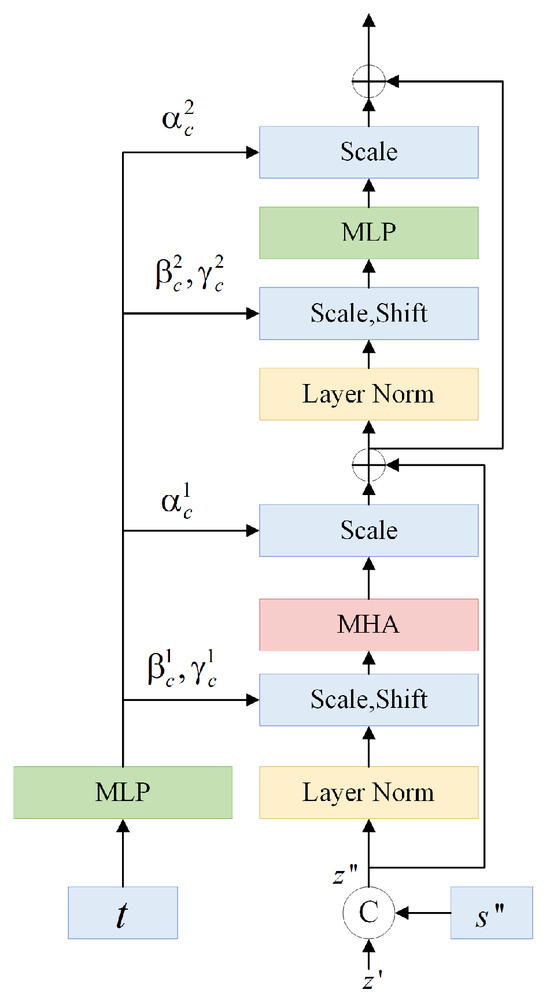
Figure 3.
Architecture of the spatial/temporal blocks in the form of a standard Transformer.
3.2.2. Reshaping Data for Transformers
The arrangement of the processed data is important to the spatiotemporal network which is detailed here. To account for it, notations are defined for the input images. B denotes the batch size, C denotes the number of bands in a image, F denotes the length of a sequence (number of images captured at different moments), H denotes the image height, and W denotes the image width. All images share the same height and width.
SAR and optical images are encoded, rearranged, and concatenated ahead of the encoding process. The input SAR sequence is arranged as . In the training stage, a sequence of target optical images is used and arranged as . After is encoded by the VAE, the optical feature in the latent space is arranged as , where , , and are the channel number, the height, and the width of features encoded by the VAE, respectively. is then patchified to the sequence ready for the network, where and are the numbers of patches horizontally and vertically, respectively, and d is the length of each token. is conditionally branched to obtain the spatiotemporal features . Similarly, is patchified into the sequence . The encoded SAR sequence and the optical sequence are added with trainable positional code p independently. They are then catenated at the last dimension to get and go through a linear layer to get , which will be fed into the backbone network.
Data also need to be rearranged when they are processed by the spatiotemporal blocks, even if they share the same Transformer structure. Image features are reshaped to ahead of spatial blocks and ahead of temporal blocks. Since the spatiotemporal blocks are alternating between each other, the reshaping operation is needed before each spatiotemporal block.
3.2.3. Embedding Time Stamp and Diffusion Step
Two timestamps are integrated into our model as follows: the diffusion step and the acquisition time of SAR images. The diffusion model broadcasts the diffusion step to guide the diffusion process. Additionally, the acquisition time of SAR images is embedded to prevent incorrect trend predictions. These timestamps need to be incorporated into the network, and they are coded and embedded in distinct ways.
The encoding and embedding of the diffusion step follows the common operation. To encode the diffusion step, The method in DDPM [27] is used, which consists of a sine–cosine coding and an MLP. The embedding of the encoded diffusion step uses the adaptive normalization in Diffusion Transformer (DiT) [29].
The coding of the capturing moments for SAR images was similar to that of the diffusion step, but a different embedding strategy was subsequently used. By setting 1 January of each year as the start, the image time is converted into the number of days from the start. Then the SAR time is converted into a high-dimensional vector using the same coding method as the diffusion step (sine–cosine coding with MLP), where B is the batch size, F is the length of a sequence, and d is the length of the vector from a patch ready for the spatiotemporal blocks. A typical d is when a image is encoded by the VAE to . The size of the encoded time is the same as the size of each patch extracted by patchify and can be embedded as a token vector ahead of the first patch. To match the cycle of seasons, the maximum period in the sine–cosine coding is set to 366.
After the image time is encoded, it will be embedded into spatiotemporal blocks. As the spatiotemporal blocks are alternating, the encoded timestamps also needs to be reshaped before embedding, such that they are in line with the organization of the spatial and temporal features ready for the next Transformer. For a spatial block, the encoded timestamp is reshaped to , which is concatenated with the image feature to obtain . For a temporal block, the encoded timestamp is reproduced to (row repetition first), which is concatenated with the image feature to obtain .
3.3. Loss Function
The MSE loss and the KL loss are used to train the proposed conditional diffusion model. The total loss is defined as
where is the normalized Gaussian noise obtained from sampling, denotes the noise estimator with parameter , t is the diffusion step, is the optical image sequence added by the Gaussian noise at the step t, y is the SAR image sequence for reference, and is the difference between two distributions. is calculated with
where denotes the mean value for a matrix, denotes the mean value, and denotes the variance.
4. Experimental Scheme
4.1. Datasets
The existing SAR-to-optical image translation datasets are all single-image translation datasets, which cannot be used for sequence image generation. In order to produce an optical image sequence from a SAR image sequence, this paper constructs two cloud-free datasets, which are named as Sequential Sentinel 1 to 2 dataset in Four Corners, Australia (SeqSen12-FCA) and Sequential Sentinel 1 to 2 in Paris, France (SeqSen12-Paris). In these datasets, the source data are from Sentinel-1, and the target data are from Sentinel-2. For each dataset, images share the same locations and ground resolutions.
Data details are listed. The ground resolution is 10 m. Sentinel-1 images are the ground range detected (GRD) products captured at the Interferometric Wide swath (IW) mode in dual-polarization (VV and VH) channels. GRD data are recorded in the double precision format ranging from 0 to 1. The Sentinel-2 images have the red, green, and blue bands stored in the unsigned integer format with the quantization range of 0–10,000. Preprocessing of the Sentinel-1 data includes orbit correction, thermal noise removal, radiometric calibration, speckle noise removal (with the Refined Lee filter), and terrain correction. The Sentinel-1 images were geographically cropped towards Sentinel-2 images. Registration [30,31] is necessary if the paired images are not geographically matched.
4.1.1. Sequential Sentinel 1 to 2 Dataset in Four Corners, Australia (SeqSen12-FCA)
This dataset’s location is Four Corners, New South Wales, Australia (34°49′32.78″S, 145°24′47.55″E). The Sentinel-1 images in the SeqSen12-FCA dataset were captured on 9 January, 14 February, 10 March, 3 April, 2 June, 14 June, 1 August, 13 August, 6 September, 24 October, 17 November, and 23 December 2021, respectively. The matched Sentinel-2 images were captured on 10 January, 9 February, 6 March, 5 April, 30 May, 19 June, 29 July, 18 August, 2 September, 27 October, 16 November, and 26 December 2021, respectively. The image size is 8960 × 8960 in the training set and 1280 × 1280 in the testing set. Images used for training and for testing are geographically non-overlapped. The center of the testing sequence used for SeqSen12-FCA locates at 34°26′8.44″S, 145°49′32.52″E.
4.1.2. Sequential Sentinel 1 to 2 Dataset in Paris (SeqSen12-Paris)
This dataset’s location is Paris, France (49°9′26.38″N, 2°22′50.73″E), used for city reconstruction. The Sentinel-1 images were captured on 3 April, 27 April, 2 June, 14 June, and 20 July 2021, respectively. The corresponding Sentinel-2 images were captured on 31 March, 25 April, 30 May, 14 June, and 9 July 2021, respectively. The image size is 8960 × 8960 in the training set and 1280 × 1280 in the testing set. Images for training and for testing are geographically non-overlapped. The center of the testing sequence used for SeqSen12-Paris locates at 49°0′14.64″N, 2°55′57.33″E.
4.2. Methods for Comparison
Since there is no research on sequence SAR-to-optical translation, the proposed method was compared with three state-of-the-art single SAR-to-optical translation algorithms, including Pix2Pix [32], ICGAN [17], and CDDPM [8]. As for the parameter settings, the parameters in [33] was referenced for Pix2Pix, whereas the ICGAN and CDDPM models used their default parameters. The input size is 256 × 256 for Pix2Pix and ICGAN whereas 64 × 64 for CDDPM.
The parameter amounts and the training time for 200 epoches on the SeqSen12-FCA dataset are given in Table 1. The parameter amount of our model is close to that of CDDPM. However, CDDPM requires 64 × 64 input size to maintain acceptable performance, whereas the use of VAE enables our method to accept 256 × 256-sized images as the input. This results in significantly fewer training patches than CDDPM, leading to reduced training time. Importantly, our approach has inherent potential of large foundation models capable of training on huge datasets.

Table 1.
Parameter amount and training time of algorithms on the SeqSen12-FCA dataset.
The parameters of our method are listed here. Each sequence contains images of four moments. The image sizes of the input and output are 256 × 256. The AdamW approach was used as the optimizer with parameter , . The proposed method was trained for 200 epochs, in which the batch size is 8 and the learning rate is 0.0001. NVIDIA Telsa A100 was used for training and testing.
4.3. Metrics
The translated images were evaluated using various metrics to assess the radiometric accuracy, structural consistency, and spectral fidelity. Radiometric accuracy was assessed using Root Mean Square Error (RMSE). Structural consistency was measured with the Structural Similarity (SSIM) index. To obtain SSIM, the red, green, and blue channels of an image were equally converted to a grayscale image. Spectral fidelity was evaluated using the Q4 index [34]. The ideal values are 1 for SSIM and Q4 and 0 for RMSE.
5. Experimental Results
All methods were independently trained and tested on two newly designed datasets. In addition, the new algorithm was tested for single SAR-to-optical translation to verify its feasibility. Both sequential and single results were evaluated with the metrics judging radiometric, structural, and spectral fidelity. The sequential results are partly demonstrated for visual comparison. Furthermore, the effectiveness of the proposed network architecture was validated through an ablation study.
5.1. Sequential Translation on the SeqSen12-FCA Dataset
The results of sequence translation for the SeqSen12-FCA dataset are presented in Table 2. To obtain this results, SAR data of every four consecutive moments were sent to the network to obtain four consecutive optical images. These four consecutive moments are monotonically increasing. When the time reaches December, January is subsequently used to loop. Thus, we can obtain twelve groups of training and testing data where the recording moments are cyclically incremented.
Table 2.
Sequential translation on the SeqSen12-FCA dataset.
Table 2 demonstrates that our method has advantage in radiometric accuracy. By setting our algorithm as the benchmark, the average RMSE errors of competing algorithms are 6.35%, 12.57%, and 6.10% higher, respectively. Pix2Pix outperforms ICGAN and CDDPM concerning radiometric and structural consistency. The performance is steady for this test with and without time stamps.
Our approach barely win for structure preservation. Overall, the structural similarity of algorithms is very close. Scores between algorithms are within 1%. Pix2Pix wins structural consistency for some scenes. The time stamp gives a weak improvement in the average SSIM. The advantages of our method in maintaining spectral continuity can be seen from Table 2. The spectral fidelity of our method outperforms the competing algorithms for all scenarios. Using our algorithm as a benchmark, the average Q4 consistency of the competitive algorithms are 44.78%, 22.87%, and 25.82% lower, respectively. Among the comparative algorithms, the spectral accuracy of ICGAN outperforms that of Pix2Pix and CDDPM. The introduction of timestamps increases spectral fidelity by 2.02%.
5.2. Sequential Translation on the SeqSen12-Paris Dataset
Table 3 shows the results obtained from training and testing using the SeqSen12-Paris dataset. The dataset contains data from 5 months (March to July). By excluding one month and using the remaining four months for training and testing, we can obtain five pairs of training and testing data. In each dataset, the four months are sorted cyclically for training and testing, such as 3/4/5/6 or 6/7/3/4. Compared to SeqSen12-FCA, SeqSen12-Paris has more complex scenes as it is partially covered by urban areas.
Table 3.
Sequential translation on the SeqSen12-Paris dataset.
Table 3 shows that our method has significant advantages for the SeqSen12-Paris dataset in terms of radiometric accuracy, structural similarity, and spectral fidelity. Using our algorithm as a benchmark, the average RMSE errors of the other algorithms increase by 56.71%, 37.35%, and 89.72%, respectively. The average SSIM decreases by 5.52%, 3.15%, and 11.79%, respectively. The average Q4 decreases by 37.76%, 26.30%, and 48.34%, respectively. By comparing Table 2 and Table 3, the significant numerical difference of the comparison algorithms indicates that they are not good at predicting content containing mixed structures. In contrast, our scores in Table 2 and Table 3 are similar, indicating the stability of the proposed method.
Table 3 also shows the value of introducing time stamps into the sequence model. When the capturing time is informed, The RMSE loss decreases by 5.28%, The structural similarity increases by 0.62%, and the spectral fidelity increases by 1.86%. It is therefore inferred that the time stamps are extraordinarily useful for this scenario.
5.3. Single Translation on Both Datasets
Our method can be used for single SAR-to-optical image translation too, although it is not deliberately designed for this purpose. To explore the feasibility of our method for single-image translation, an additional experiment was added. In this experiment, single images were used as the input and output of our method. The experiment was tested on the SeqSen12-FCA and SeqSen12-Paris datasets. The scores of the experimental results are presented in Table 4 and Table 5.
Table 4.
Single translation on the SeqSen12-FCA dataset.
Table 5.
Single translation on the SeqSen12-Paris dataset.
Table 4 shows that our method is slightly superior to other algorithms when used for single-image farmland reconstruction, where the time stamp plays an important role. Due to the repeated use of results from single-image translation algorithms, the average scores of the competing algorithms in Table 4 are the same as the scores of the sequence translation in Table 2. Compared to the scores of sequence translation, our method degrades by 3.38% for the single translation. Compared with our algorithm, the RMSE errors of the comparison algorithms are 2.87%, 8.89%, and 2.63% larger. Our method still has advantages in spectral preservation, but it degrades by 14.5% if compared to sequence translation. The Q4 scores of the comparison algorithms are 35.43%, 9.79%, and 13.25% lower than ours.
The conclusion from Table 5 is very similar to that from Table 4, which once again confirms that our method’s performance will significantly decrease when used for single-image translation. The largest degradation is for spectral fidelity, where it is outweighed by ICGAN. Our method still maintains a leading position for radiometric and structural reconstruction, but the gap against our competitors has significantly narrowed. Compared to Table 3, the degradation of radiometric accuracy, structural similarity, and spectral fidelity are 29.67%, 2.08%, and 27.37%, respectively.
Interestingly, Table 4 and Table 5 uncover that the introduction of time stamps has a greater improvement for single-image translation. In Table 4, 7 out of 12 months shows improved performance with the introduction of time stamps. In Table 5, all months shows improved performance after introducing time stamps. This can be explained as the time stamp indicates the target time which reduces the decoding errors.
5.4. Visual Comparison of Sequential Translation on Two Datasets
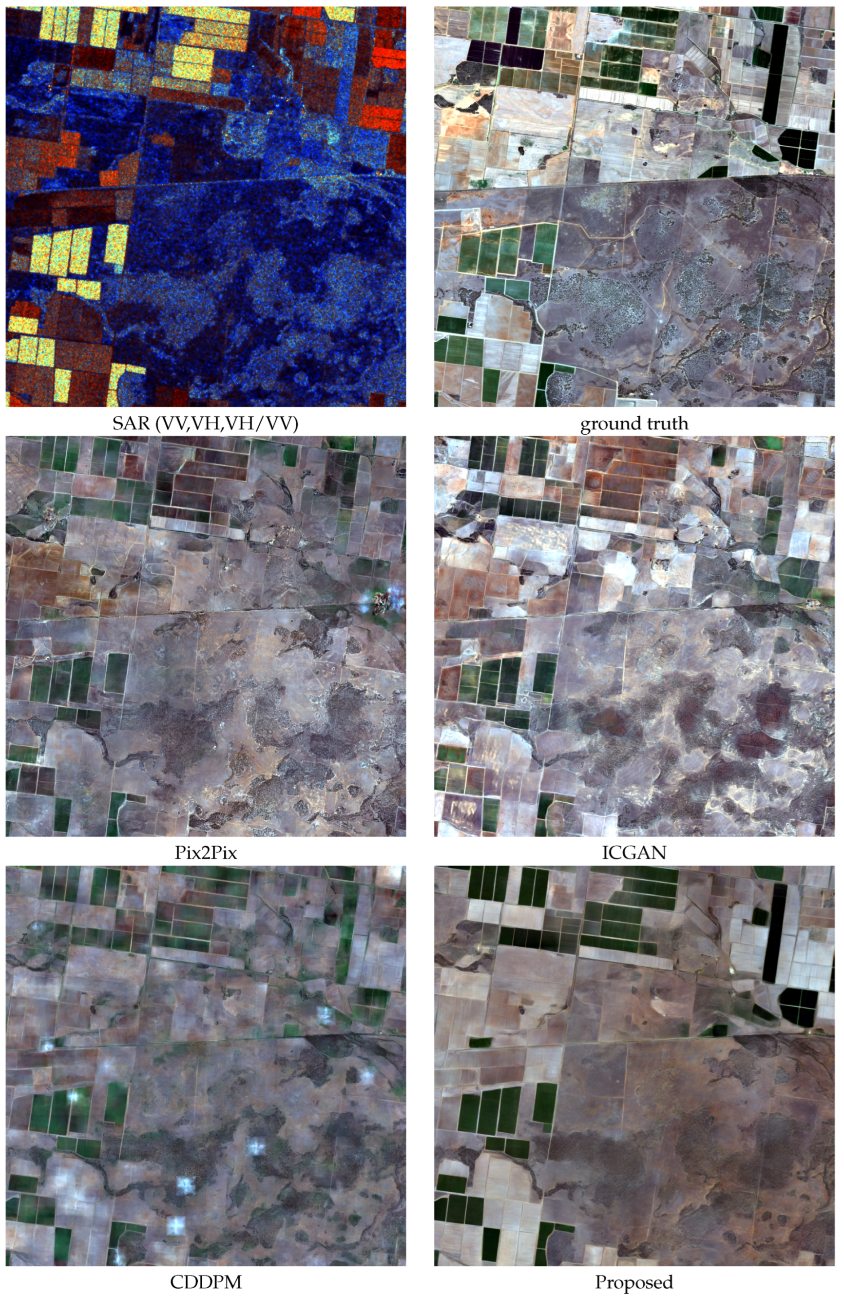
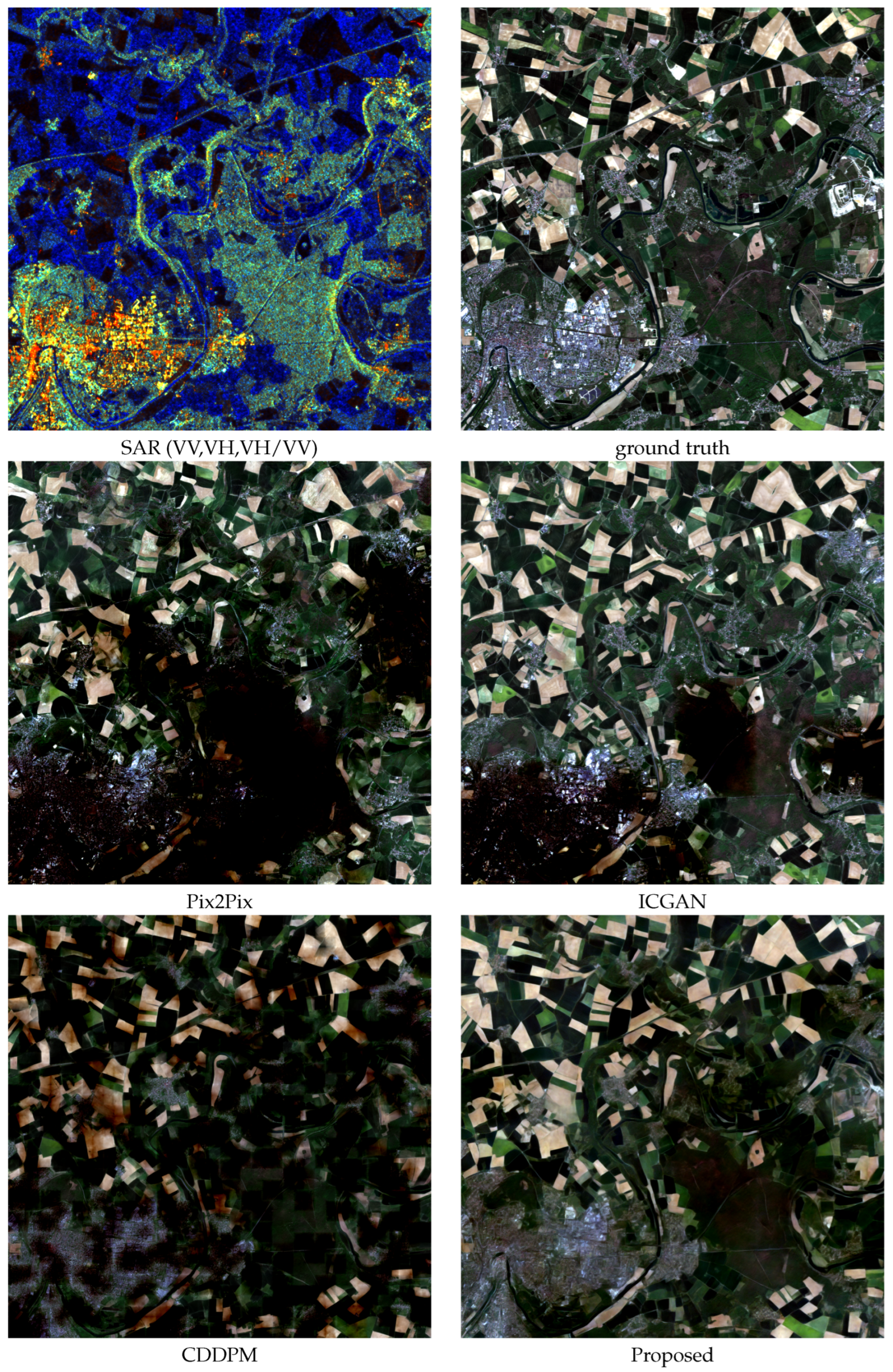
Some of the reconstruction results are presented in Figure 4 and Figure 5 for perceptual judgment. The January results are chosen for the SeqSen12-FCA dataset, and the April results are chosen for the SeqSen12-Paris dataset. Our results are averaged across the four images generated from different reference sequences, and they agree very well with the single image as a whole. However, some details are blurred and small details are removed while smoothing out the noise. All images were nonlinearly enhanced by the 2% saturation stretching in which the thresholds are the same as the ground truth images. With the uniform thresholds, the radiometric and spectral deviations can be read out from the images directly.
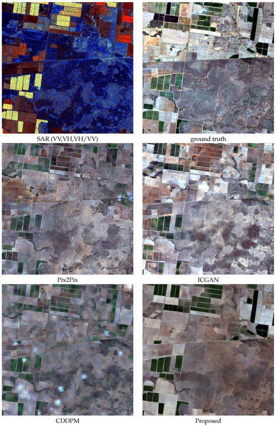
Figure 4.
January’s average results of sequential SAR-to-optical translation on the SeqSen12-FCA dataset.

Figure 5.
April’s average results of sequential SAR-to-optical translation on the SeqSen12-Paris dataset.
Figure 4 shows the January test results for the SeqSen12-FCA dataset. In terms of spectral fidelity, ICGAN fails to restore the green regions well. Our method has a advantage in spectral accuracy as it restore the dark regions on the upper right successfully. As for the structure, Pix2Pix and ICGAN provide very sharp details. In contrast, CDDPM and our method have less details. However, the structures of Pix2Pix and ICGAN are clearly reproduced from the SAR image deviating from the optical image.
Figure 5 shows the April results tested for the SeqSen12-Paris dataset. For radiometric and spectral fidelity in suburban areas, ICGAN and our method can restore farmland (in green) and bare ground (in yellow) accurately, while CDDPM suffers from severe radiometric inaccuracies. For the radiometric and spectral consistency of urban areas, only our method can restore them well. In terms of structure, all algorithms reconstruct the suburb areas well, but they have difficulty in reconstructing urban areas. Pix2Pix and ICGAN produce more details than CDDPM and our method.
Figure 4 and Figure 5 show that the sequential method has advantages in restoring the overall brightness of each image block. CDDPM and our method are diffusion models. The dark results of CDDPM indicate the brightness loss, and it varies greatly from block to block. As a comparison, the uniformity and accuracy of the brightness of our results are far better. For this purpose, sequence generation plays a key role as it provides more information.
5.5. Ablation Study
Compared to a standard conditional diffusion model, the primary enhancement in this study is the integration of temporal disciplines and time marks for reconstruction. The ablation study tries to uncover the feasibility and impact of the temporal blocks and time stamps. After some branches of the proposed method were removed, the remaining models were trained and tested with the SeqSen12-FCA and SeqSen12-Paris datasets, respectively, and the results were evaluated. The parameters were kept as for the standard model. The results are presented in Table 6 and Table 7, which confirm the value of introducing temporal blocks and time stamps for SAR-to-optical translation.
Table 6.
Ablation study: Sequence translation for the SeqSen12-FCA dataset.
Table 7.
Ablation study: Sequence translation for the SeqSen12-Paris dataset.
6. Discussions
6.1. Replacing Transformer with Mamba
Mamba [35] is a recently proposed sequence modeling tool. It has linear time complexity and can handle longer sequences. Due to the removal of the attention module, Mamba requires significantly less GPU memory than Transformer. To validate the feasibility of Mamba for our model, we replace the Transformer in our model directly with the Mamba2 model [36]. Mamba2 is an improved Mamba with smaller model size under the same performance. In addition, Mamba2 is able to utilize a larger state dimension, further enhancing its ability to handle complex tasks, especially those that require high-capacity states.
The experiment using Mamba2 for sequential translation was tested on SeqSen12-FCA, and the results are shown in Table 8. Unfortunately, the scores are far lower than using Transformer. The reason may be that our sequence length is only four, which cannot fully utilize the advantages of Mamba2 in modeling long sequences.
Table 8.
Sequence translation for the SeqSen12-FCA dataset with Mamba blocks.
6.2. Limitations and Potentials
The translation results cannot be used for quantitative remote sensing yet. In addition to sequential translation, single-image translation was also tested in this work. The relative radiometric error is defined as the RMSE divided by the mean value of the ground truth image. At present, the relative radiometric error of single-image translation exceeds 30%. Our sequential translation has reduced the relative radiometric error to within 25%. However, the relative radiometric error allowed for quantitative remote sensing should be within 10% or even smaller.
On the other hand, the sequential translation has potential in practice. The current translation quality is applicable for interpretation purposes (e.g., classification and segmentation) or other visual purposes, as the structural similarity is over 0.9. Sequential translation can also be improved with new references. For example, possible optical references can undoubtedly improve the translation quality. Where the GRD data source is concerned, it is promising with single-look complex data for translation by exploiting the phase information as reference and polarimetric decomposition for coherency.
7. Conclusions
In this paper, we focus on translating a SAR image sequence to an optical image sequence, and we solved it with diffusion networks. This work may represent the first effort in sequence translation that incorporates time-series images along with their respective capture times. Following the diffusion framework, we employed twelve Transformers as the backbone to estimate the noise in the image features, which were preprocessed using a variational autoencoder. Additionally, a conditional branch was designed specifically for SAR sequences to extract relevant features. The capture time was encoded and integrated into the Transformers.
Since the existing translation datasets were designed for single translations, two new datasets were created for sequence translation. The Sentinel-1 GRD data served as the SAR source, while the Sentinel-2 red, green, and blue (R/G/B) data acted as the optical source. Experiments were conducted on the two datasets using sequence translation, single translation, and ablation studies. The translation results were compared with three single translation algorithms. The scores indicate that when sequential SAR images were utilized, the RMSE loss decreased by 3.26% and 22.9% for the two datasets, respectively. Including capturing moments helps to reduce the RMSE loss by 0.75% and 5.01% for the two datasets, respectively. In terms of visual comparison, our method demonstrates superior radiometric accuracy and spectral fidelity.
Author Contributions
Data curation, P.K.; investigation, J.W.; software, H.Z. and Y.M.; writing—original draft, J.W.; writing—review and editing, J.W. and R.T.; resources, R.T. All authors have read and agreed to the published version of the manuscript.
Funding
This research was supported by the National Natural Science Foundation of China (No. 42267070).
Data Availability Statement
The datasets used in this paper are available online https://github.com/isstncu/seqsen12 (accessed on 29 June 2025).
Conflicts of Interest
The authors declare no conflicts of interest.
References
- Ma, Y.; Wang, Q.; Wei, J. Spatiotemporal Fusion via Conditional Diffusion Model. IEEE Geosci. Remote Sens. Lett. 2024, 21, 5002405. [Google Scholar] [CrossRef]
- Wei, J.; Gan, L.; Tang, W.; Li, M.; Song, Y. Diffusion models for spatio-temporal-spectral fusion of homogeneous Gaofen-1 satellite platforms. Int. J. Appl. Earth Obs. Geoinf. 2024, 128, 103752. [Google Scholar] [CrossRef]
- Enomoto, K.; Sakurada, K.; Wang, W.; Kawaguchi, N.; Matsuoka, M.; Nakamura, R. Image Translation Between Sar and Optical Imagery with Generative Adversarial Nets. In Proceedings of the 38th IEEE International Geoscience and Remote Sensing Symposium (IGARSS), IEEE International Symposium on Geoscience and Remote Sensing IGARSS, Valencia, Spain, 22–27 July 2018; pp. 1752–1755. [Google Scholar]
- Wang, L.; Xu, X.; Yu, Y.; Yang, R.; Gui, R.; Xu, Z.; Pu, F. SAR-to-Optical Image Translation Using Supervised Cycle-Consistent Adversarial Networks. IEEE Access 2019, 7, 129136–129149. [Google Scholar] [CrossRef]
- Fu, S.; Xu, F.; Jin, Y.Q. Reciprocal translation between SAR and optical remote sensing images with cascaded-residual adversarial networks. Sci. China-Inf. Sci. 2021, 64, 122301. [Google Scholar] [CrossRef]
- Wang, Z.W.; Ma, Y.; Zhang, Y. Hybrid cGAN: Coupling Global and Local Features for SAR-to-Optical Image Translation. IEEE Trans. Geosci. Remote Sens. 2022, 60, 5236016. [Google Scholar] [CrossRef]
- Xiong, Q.; Li, G.; Yao, X.; Zhang, X. SAR-to-Optical Image Translation and Cloud Removal Based on Conditional Generative Adversarial Networks: Literature Survey, Taxonomy, Evaluation Indicators, Limits and Future Directions. Remote Sens. 2023, 15, 1137. [Google Scholar] [CrossRef]
- Bai, X.; Pu, X.; Xu, F. Conditional Diffusion for SAR to Optical Image Translation. IEEE Geosci. Remote Sens. Lett. 2024, 21, 4000605. [Google Scholar] [CrossRef]
- Pipia, L.; Muñoz-Marí, J.; Amin, E.; Belda, S.; Camps-Valls, G.; Verrelst, J. Fusing optical and SAR time series for LAI gap filling with multioutput Gaussian processes. Remote Sens. Environ. 2019, 235, 111452. [Google Scholar] [CrossRef]
- Zhao, W.; Qu, Y.; Chen, J.; Yuan, Z. Deeply synergistic optical and SAR time series for crop dynamic monitoring. Remote Sens. Environ. 2020, 247, 111952. [Google Scholar] [CrossRef]
- Roßberg, T.; Schmitt, M. Temporal Upsampling of NDVI Time Series by RNN-Based Fusion of Sparse Optical and Dense SAR-Derived NDVI Data. In Proceedings of the IGARSS 2023—2023 IEEE International Geoscience and Remote Sensing Symposium, Pasadena, CA, USA, 16–21 July 2023; pp. 5990–5993. [Google Scholar]
- Li, J.; Li, C.; Xu, W.; Feng, H.; Zhao, F.; Long, H.; Meng, Y.; Chen, W.; Yang, H.; Yang, G. Fusion of optical and SAR images based on deep learning to reconstruct vegetation NDVI time series in cloud-prone regions. Int. J. Appl. Earth Obs. Geoinf. 2022, 112, 102818. [Google Scholar] [CrossRef]
- Peng, T.; Liu, M.; Liu, X.; Zhang, Q.; Wu, L.; Zou, X. Reconstruction of Optical Image Time Series with Unequal Lengths SAR Based on Improved Sequence–Sequence Model. IEEE Trans. Geosci. Remote Sens. 2022, 60, 5632017. [Google Scholar] [CrossRef]
- Tan, D.; Liu, Y.; Li, G.; Yao, L.; Sun, S.; He, Y. Serial GANs: A Feature-Preserving Heterogeneous Remote Sensing Image Transformation Model. Remote Sens. 2021, 13, 3968. [Google Scholar] [CrossRef]
- Zhang, Q.; Liu, X.; Liu, M.; Zou, X.; Zhu, L.; Ruan, X. Comparative Analysis of Edge Information and Polarization on SAR-to-Optical Translation Based on Conditional Generative Adversarial Networks. Remote Sens. 2021, 13, 128. [Google Scholar] [CrossRef]
- Guo, J.; He, C.; Zhang, M.; Li, Y.; Gao, X.; Song, B. Edge-Preserving Convolutional Generative Adversarial Networks for SAR-to-Optical Image Translation. Remote Sens. 2021, 13, 3575. [Google Scholar] [CrossRef]
- Yang, X.; Zhao, J.Y.; Wei, Z.Y.; Wang, N.N.; Gao, X.B. SAR-to-optical image translation based on improved CGAN. Pattern Recognit. 2022, 121, 108208. [Google Scholar] [CrossRef]
- Li, H.; Gu, C.; Wu, D.; Cheng, G.; Guo, L.; Liu, H. Multiscale Generative Adversarial Network Based on Wavelet Feature Learning for SAR-to-Optical Image Translation. IEEE Trans. Geosci. Remote Sens. 2022, 60, 5236115. [Google Scholar] [CrossRef]
- Wei, J.; Zou, H.; Sun, L.; Cao, X.; He, S.; Liu, S.; Zhang, Y. CFRWD-GAN for SAR-to-Optical Image Translation. Remote Sens. 2023, 15, 2547. [Google Scholar] [CrossRef]
- Kong, Y.; Liu, S.; Peng, X. Multi-Scale translation method from SAR to optical remote sensing images based on conditional generative adversarial network. Int. J. Remote Sens. 2022, 43, 2837–2860. [Google Scholar] [CrossRef]
- Seo, M.; Oh, Y.; Kim, D.Y.; Kang, D.G.; Choi, Y. Improved Flood Insights: Diffusion-Based SAR to EO Image Translation. arXiv 2023, arXiv:2307.07123. [Google Scholar]
- Shi, H.; Cui, Z.; Chen, L.; He, J.; Yang, J. A brain-inspired approach for SAR-to-optical image translation based on diffusion models. Front. Neurosci. 2024, 18, 1352841. [Google Scholar] [CrossRef]
- Zhang, M.; Zhang, P.; Zhang, Y.; Yang, M.; Li, X.; Dong, X.; Yang, L. SAR-to-Optical Image Translation via an Interpretable Network. Remote Sens. 2024, 16, 242. [Google Scholar] [CrossRef]
- Zhang, M.; He, C.; Zhang, J.; Yang, Y.; Peng, X.; Guo, J. SAR-to-Optical Image Translation via Neural Partial Differential Equations. In Proceedings of the Thirty-First International Joint Conference on Artificial Intelligence, IJCAI-22. International Joint Conferences on Artificial Intelligence Organization, Vienna, Austria, 23–29 July 2022; pp. 1644–1650. [Google Scholar]
- Song, J.; Meng, C.; Ermon, S. Denoising Diffusion Implicit Models. arXiv 2020, arXiv:2010.02502. [Google Scholar]
- Rombach, R.; Blattmann, A.; Lorenz, D.; Esser, P.; Ommer, B. High-Resolution Image Synthesis with Latent Diffusion Models. In Proceedings of the 2022 IEEE/CVF Conference on Computer Vision and Pattern Recognition (CVPR), IEEE Conference on Computer Vision and Pattern Recognition, New Orleans, LA, USA, 18–24 June 2022; pp. 10674–10685. [Google Scholar]
- Ho, J.; Jain, A.; Abbeel, P. Denoising Diffusion Probabilistic Models. arXiv 2020, arXiv:2006.11239. [Google Scholar]
- Ma, X.; Wang, Y.; Jia, G.; Chen, X.; Liu, Z.; Li, Y.F.; Chen, C.; Qiao, Y. Latte: Latent Diffusion Transformer for Video Generation. arXiv 2024, arXiv:2401.03048. [Google Scholar]
- Peebles, W.S.; Xie, S. Scalable Diffusion Models with Transformers. In Proceedings of the 2023 IEEE/CVF International Conference on Computer Vision (ICCV), Paris, France, 1–6 October 2023; pp. 4172–4182. [Google Scholar]
- Li, L.; Han, L.; Ding, M.; Liu, Z.; Cao, H. Remote Sensing Image Registration Based on Deep Learning Regression Model. IEEE Geosci. Remote Sens. Lett. 2022, 19, 8002905. [Google Scholar] [CrossRef]
- Sommervold, O.; Gazzea, M.; Arghandeh, R. A Survey on SAR and Optical Satellite Image Registration. Remote Sens. 2023, 15, 850. [Google Scholar] [CrossRef]
- Isola, P.; Zhu, J.Y.; Zhou, T.H.; Efros, A.A. Image-to-Image Translation with Conditional Adversarial Networks. In Proceedings of the 30th IEEE/CVF Conference on Computer Vision and Pattern Recognition (CVPR), IEEE Conference on Computer Vision and Pattern Recognition, Honolulu, HI, USA, 21–26 July 2017; pp. 5967–5976. [Google Scholar]
- Zhao, Y.; Çelik, T.; Liu, N.; Li, H. A Comparative Analysis of GAN-Based Methods for SAR-to-Optical Image Translation. IEEE Geosci. Remote Sens. Lett. 2022, 19, 3512605. [Google Scholar] [CrossRef]
- Alparone, L.; Baronti, S.; Garzelli, A.; Nencini, F. A global quality measurement of pan-sharpened multispectral imagery. IEEE Geosci. Remote Sens. Lett. 2004, 1, 313–317. [Google Scholar] [CrossRef]
- Gu, A.; Dao, T. Mamba: Linear-Time Sequence Modeling with Selective State Spaces. arXiv 2023, arXiv:2312.00752. [Google Scholar]
- Dao, T.; Gu, A. Transformers are SSMs: Generalized Models and Efficient Algorithms Through Structured State Space Duality. arXiv 2024, arXiv:2405.21060. [Google Scholar]
Disclaimer/Publisher’s Note: The statements, opinions and data contained in all publications are solely those of the individual author(s) and contributor(s) and not of MDPI and/or the editor(s). MDPI and/or the editor(s) disclaim responsibility for any injury to people or property resulting from any ideas, methods, instructions or products referred to in the content. |
© 2025 by the authors. Licensee MDPI, Basel, Switzerland. This article is an open access article distributed under the terms and conditions of the Creative Commons Attribution (CC BY) license (https://creativecommons.org/licenses/by/4.0/).