Estimating Subsurface Geostatistical Properties from GPR Reflection Data Using a Supervised Deep Learning Approach

Abstract

The quantitative characterization of near-surface heterogeneity using ground-penetrating radar (GPR) is an important but challenging task. The estimation of subsurface geostatistical parameters from surface-based common-offset GPR reflection data has so far relied upon a Monte-Carlo-type inversion approach. This allows for a comprehensive exploration of the parameter space and provides some measure of uncertainty with regard to the inferred results. However, the associated computational costs are inherently high. To alleviate this problem, we present an alternative deep-learning-based technique, that, once trained in a supervised context, allows us to perform the same task in a highly efficient manner. The proposed approach uses a convolutional neural network (CNN), which is trained on a vast database of autocorrelations obtained from synthetic GPR images for a comprehensive range of stochastic subsurface models. An important aspect of the training process is that the synthetic GPR data are generated using a computationally efficient approximate solution of the underlying physical problem. This strategy effectively addresses the notorious challenge of insufficient training data, which frequently impedes the application of deep-learning-based methods in applied geophysics. Tests on a wide range of realistic synthetic GPR data generated using a finite-difference time-domain (FDTD) solution of Maxwell’s equations, as well as a comparison with the results of the traditional Monte Carlo approach on a pertinent field dataset, confirm the viability of the proposed method, even in the presence of significant levels of data noise. Our results also demonstrate that typical mismatches between the dominant frequencies of the analyzed and training data can be readily alleviated through simple spectral shifting.

1. Introduction

The shallow subsurface consists of soil, glacial and alluvial deposits, as well as weathered bedrock. It is from this thin, surficial layer that we draw our drinking water and produce our food, and it is where we ultimately discharge much of our waste. In densely populated and highly industrialized regions, the sustainable use of this increasingly fragile surficial environment has become a societal and political issue of critical importance. Near-surface geophysics, in general, and ground-penetrating radar (GPR) in particular allow for the exploration and characterization of this surficial environment and thus have an essential role to play in this endeavor.

Surface-based GPR reflection profiling has the potential to provide images of shallow subsurface structure with unsurpassed spatial resolution. However, due to the inherently complex and heterogeneous nature of the surficial environment, these images are often better suited to stochastic than to deterministic interpretation approaches. This means that we aim to estimate parameters describing the geostatistical nature of heterogeneity. Specifically, the second-order statistical properties of GPR reflection data are expected to provide information about the correlation structure of the subsurface velocity field through which the high-frequency electromagnetic waves have traveled. Rea and Knight and Dafflon et al. observed a far-reaching qualitative agreement between the spatial correlation structure of cliff-face photographs and those of GPR images collected along the tops of the cliffs [1,2]. This led them to conclude that the lateral statistics of a GPR image and the underlying water content distribution are directly related. Knight et al. also found similarities between the lateral correlation statistics of GPR data and neutron probe measurements [3]. However, Knight et al. and Oldenborger et al. noticed that the lateral correlation structure of a GPR image is significantly affected by its vertical resolution, which is controlled by the frequency content of the emitted source signal [4,5]. These findings indicate that the assumption of a direct relation, let alone an equivalence, between the lateral statistics of water content and GPR reflection data is not valid and that the physics of the underlying wave propagation phenomena should be accounted for more appropriately. Irving et al. and Irving and Holliger followed up on these pioneering studies, notably by clarifying the underlying theoretical and methodological foundations [6,7]. They found that GPR reflection images allow us to infer the structural aspect ratio $a_x/a_z$ of the subsurface heterogeneity, whereas the associated values of the horizontal and vertical correlation lengths $a_x$ and $a_z$ cannot be independently resolved. GPR data also seem to exhibit only a weak sensitivity to the decay of the associated power spectrum. These findings have been corroborated through a wide range of follow-up studies not only for GPR [8,9], but also for seismic reflection data [10,11]. In this context, it is important to note that knowledge regarding the structural aspect ratio $a_x/a_z$ of the underlying heterogeneity is essential for the geostatistical characterization of the probed subsurface region, as this information cannot be easily inferred otherwise. The vertical correlation length $a_z$ as well as the spectral decay of the power spectrum, in contrast, can often be estimated using logging data from nearby boreholes [9,12]. Geostatistical parameters such as correlation lengths and structural aspect ratio provide a description of small-scale subsurface heterogeneity. In GPR inversion, these parameters can serve as prior information to guide the selection of regularization parameters and reduce solution non-uniqueness [13]. In hydrogeological modeling, the spatial heterogeneity of subsurface media is typically represented as a random field, and these parameters act as key inputs to stochastic flow and transport models. They help to characterize the spatial structure of hydraulic properties and thereby influence predictions of groundwater flow and contaminant transport.

To date, the estimation of subsurface geostatistical parameters from reflection GPR data has been based on Monte-Carlo-type inversion approaches (e.g., Irving et al., 2009; Xu et al., 2020), whereby sets of model parameters drawn from prescribed prior distributions are either accepted or rejected depending on how well they allow for prediction of the observed autocorrelation structure of the GPR image. While this approach has the advantage of allowing for a comprehensive exploration of the model parameter space and providing a corresponding estimate of uncertainty, the associated computational costs are high, in particular for 3D datasets [6,8]. In this work, we seek to explore a potential alternative using a fundamentally different approach based on supervised deep learning. Deep learning techniques employ multi-layer artificial neural networks, especially convolutional neural networks (CNN), to unravel complex relationships between input and output [14,15]. In recent years, these methods have attracted increasing attention in the geophysical community as a novel data-driven technique compared to conventional model-driven approaches [16,17,18]. For wave-based geophysical exploration techniques, such as seismic and GPR reflection imaging, deep learning has demonstrated remarkable utility in many areas, including data processing [19,20,21], interpretation [22,23], and inversion [24,25,26].

Here, we explore the use of a standard CNN architecture to establish a relationship between the spatial autocorrelations of surface-based GPR reflection images and the geostatistical parameters characterizing the distribution of the dielectric permittivity in the probed subsurface region. An important aspect of our workflow is that the training of the CNN is based on synthetic GPR reflection data, which are generated using a computationally highly efficient convolution-based modeling technique. While the latter is clearly an approximation of the underlying physics of high-frequency electromagnetic wave propagation, it is generally considered adequate for small incidence angles and has proven to be highly effective in previous waveform-based GPR inversion studies [9,13,27]. In the following, we first present the methodological foundations of our proposed approach, followed by its validation for realistic synthetic GPR data generated using a finite-difference time-domain (FDTD) solution of Maxwell’s equations. We then examine the impact of noise on the estimation process and how typical spectral mismatches between the training database and the analyzed data can be accounted for. Finally, we apply the proposed method to an observed GPR dataset from a typical surficial alluvial environment and compare the results with those obtained using the well-established Monte-Carlo-based inversion approach.

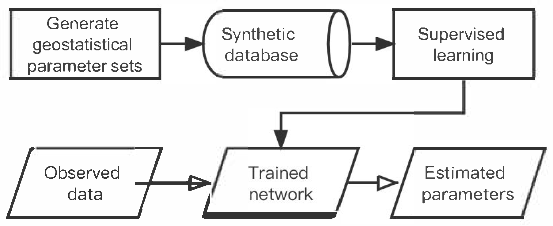
2. Methodology

The overall idea behind our proposed approach is as follows: (i) to generate a vast synthetic GPR database for a comprehensive range of stochastic subsurface models; (ii) to train a CNN in a supervised setting in order to build a link between the 2D autocorrelation images of the synthetic images and the targeted geostatistical parameters of the probed subsurface region; and (iii) to use the trained CNN to estimate the geostatistical parameters corresponding to a particular GPR dataset from its 2D autocorrelation image (Figure 1). A distinction of our approach compared to other deep learning applications in GPR research is that the input to the network is not the GPR reflection data themselves, but their 2D spatial autocorrelation. This transformation enables the CNN to more directly extract information related to subsurface geostatistical parameters.

2.1. Geostatistical Background

A fundamental assumption underlying our work is that the key characteristics of the prevailing subsurface heterogeneity can be adequately described by its second-order statistics. Our experience from previous Monte-Carlo-based inversions for near-surface geostatistical parameters, as well as evidence from the characterization of hydrocarbon reservoirs, indicate that, to a first approximation, this is generally the case as long as the analysis focuses on a given lithological and/or hydraulic unit [1,6,7,8,9]. To relate the second-order statistics of the electromagnetic velocity structure of the subsurface to the corresponding GPR reflection image, we briefly summarize the essential elements of the derivation presented in Irving et al. [9]. We begin with the assumption that the subsurface electromagnetic velocity distribution $v\left(x,z\right)$ can be characterized as the superposition of a slowly varying or constant background velocity model $v_0\left(x,z\right)$, upon which small-scale stochastic fluctuations $∆v(x,z)$ are superposed as follows:

$$v(x,z)=v_0(x,z)+∆v(x,z).$$

(1)

It is the stochastic component of the velocity structure $∆v(x,z)$ that gives rise to the reflected GPR wavefield recorded at the surface and whose second-order statistics we wish to estimate. To this end, the underlying subsurface GPR reflectivity distribution $r(x,z)$ can be approximated as the vertical derivative of the velocity perturbation field [28,29]

$$r(x,z)\approx {\displaystyle \frac{\mathsf{\partial }}{\mathsf{\partial }z}}∆v(x,z).$$

(2)

Assuming that the recorded GPR wavefield is largely non-dispersive and dominated by single scattering, a typical common-offset GPR reflection section, after processing and migration, can be approximated as the convolution of the subsurface reflectivity r with the source wavelet w as well as with a filter h that accounts for the limited lateral resolution of the GPR image [6,10].

$$\begin{array}{ll}p\left(x,z\right)& =w\left(z\right) \ast r\left(x,z\right) \ast h\left(x\right)\\ & =w\left(z\right) \ast {\displaystyle \frac{\mathsf{\partial }}{\mathsf{\partial }z}}∆v\left(x,z\right) \ast h\left(x\right)\\ & =∆v\left(x,z\right) \ast f\left(x,z\right),\end{array}$$

(3)

where $p\left(x,z\right)$ is the so-called primary reflection section and $f\left(x,z\right)={\displaystyle \frac{\mathsf{\partial }}{\mathsf{\partial }z}}w\left(z\right) \ast h(x)$.

Equation (3) provides a simple convolutional relationship between the velocity perturbation field $∆v\left(x,z\right)$ and the GPR reflection image $p\left(x,z\right)$. Making use of the Fourier transform and the Wiener–Khinchin theorem linking the power spectrum and autocorrelation functions, a similar convolutional relationship is implied for the spatial autocorrelations of all quantities.

$$R_{pp}\left(\delta x,\delta z\right)=R_{vv}\left(\delta x,\delta z\right) \ast R_{ff}\left(\delta x,\delta z\right).$$

(4)

Equation (4) states that the 2D spatial autocorrelation of the GPR image $R_{pp}\left(\delta x,\delta z\right)$, where $\delta x$ and $\delta z$ refer to the horizontal and vertical lags, respectively, is related to the 2D spatial autocorrelation of the velocity perturbation field $R_{vv}\left(\delta x,\delta z\right)$ through 2D convolution with the filter autocorrelation $R_{ff}\left(\delta x,\delta z\right)$. This equation provides an effective link between the second-order statistics of the high-frequency electromagnetic wave velocity field with those of the corresponding GPR reflection section. Based on this link, we use 2D autocorrelation images of GPR reflection data $R_{pp}$ to train our CNN to predict the geostatistical parameters governing $R_{vv}$.

To describe the expected range of near-surface subsurface velocity heterogeneity, we consider the highly versatile von Karman autocorrelation function [30], which is particularly well-established for this purpose [8,9,12,31] and given by the following:

$$R_{vv}\left(\delta x,\delta z\right)={\displaystyle \frac{r^v{K}_v\left(r\right)}{2^{v-1}\Gamma (v)}},$$

(5)

where $K_v\left(r\right)$ is the modified Bessel function of the second kind of order $0\le v\le 1$, $\Gamma$ is the gamma function, and

$$r=\sqrt{{(x/a_x)}^2+{(z/a_z)}^2}$$

(6)

is the weighted radial autocorrelation lag with $a_x$ and $a_z$ denoting the horizontal and vertical correlation lengths, respectively. The $v$-value, also known as the Hurst number, determines the slope of the power spectrum $P_{vv}=\mathcal{F}\left\{R_{vv}\right\}$, with $\mathcal{F}$ denoting the Fourier transform, or, equivalently, the rate of decay of the autocorrelation $R_{vv}$ at short lags [32]. Values of v close to zero characterize the seemingly ubiquitous pink or flicker noise. A value of $v$ = 0.5 corresponds to the well-known exponential correlation function describing brown noise. Finally, for v-values close to 1, which characterize so-called black noise, the von Karman autocorrelation function resembles its Gaussian equivalent.

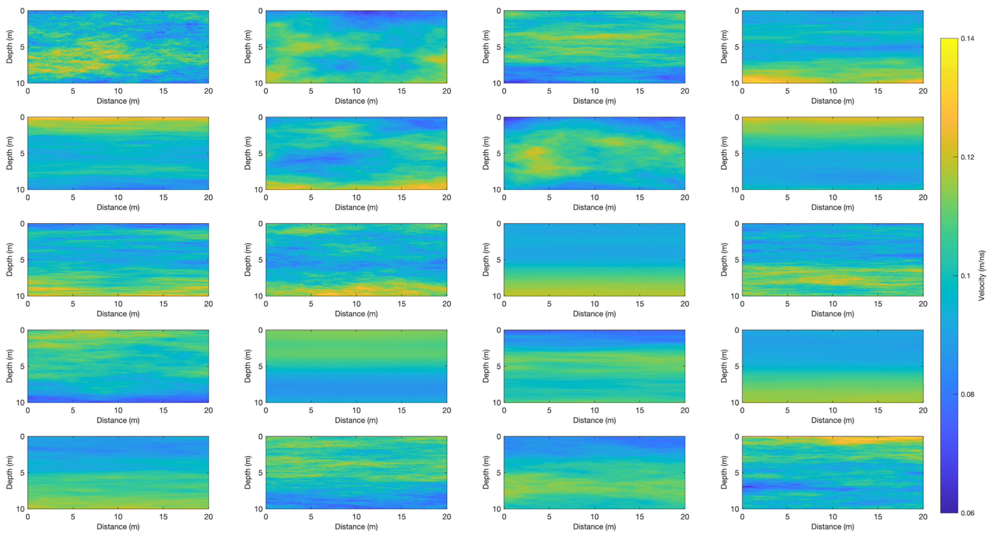
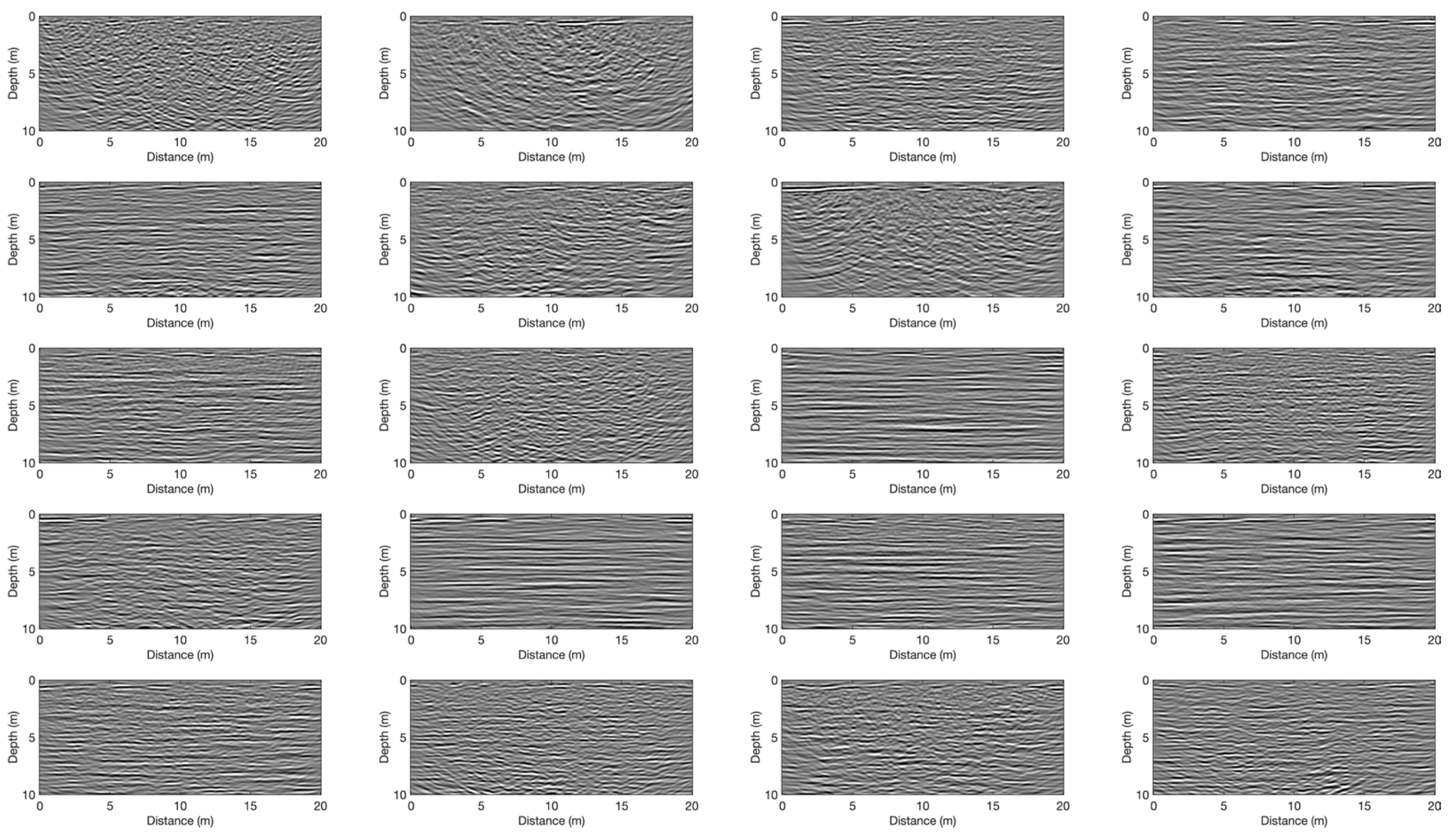
2.2. Generation of Training Database

Based on the von Karman autocorrelation function described in Equation (5), we generated 3000 stochastic subsurface GPR velocity models representing a wide range of combinations of $a_x$, $a_z$, and $v$. The models are 20 m wide and 10 m deep. We considered values of $a_z$ ranging from 0.1 to 1 m, and we chose the aspect ratio $a_x/a_z$ within the range of 1 to 20, which allowed us to achieve the corresponding values of $a_x$. The $v$-value varies between 0.1 and 0.9. Stochastically layered models of this kind are widely regarded as being characteristic of surficial alluvial environments [8,9,12,33]. For all 3000 realizations, the values of $a_z$, $a_x/a_z$, and $v$ were chosen randomly, while the mean value of the velocity and its standard deviation are fixed at 0.1 m/ns and 0.01 m/ns, respectively. In addition, we generated 100 additional stochastic models using the same method for validation during network training.

From the subsurface velocity models, we generated corresponding synthetic GPR reflection images by convolving the vertical reflectivity series at all transmitter–receiver locations, spaced at 0.1 m, with a Ricker source wavelet having a central frequency of 100 MHz. This is followed by the application of a Gaussian filter h(x) (Equation (3)) with a width of approximately one dominant wavelength to emulate the limited lateral resolution of a migrated GPR image [7]. It is important to note that we use this approximate convolution method to generate our synthetic database because it has a much lower computational cost than comprehensive approaches to solve Maxwell’s equations, such as the FDTD method. The generation of the 3000 training datasets takes only tens of seconds on a 2018 MacBook Pro (Apple Inc., Cupertino, CA, USA). Although the convolution model does not capture the full physics of a GPR reflexion experiment, previous work has shown that it is capable of emulating a remarkable degree of realism present in GPR field data, even in complex scenarios [9,13]. The resulting synthetic GPR data were contaminated with zero–mean Gaussian random noise having a standard deviation of 2% with regard to the maximum absolute amplitude of the synthetic data.

2.3. Supervised Learning

We computed the 2D autocorrelations of the 3000 synthetic GPR reflection images, which we then used together with the corresponding values of $a_x/a_z$ to perform the supervised training of the CNN. Figure 2 shows an example of a stochastic subsurface velocity model characterized by $a_x=2$ m, $a_z=0.2$ m, and $v=0.5$ (Figure 2a), the corresponding synthetic convolution-based GPR image (Figure 2b), and its 2D autocorrelation function (Figure 2c). For the design and training of the CNN, we employed the MATLAB R2016 Deep Learning Toolbox (MathWorks, Natick, MA, USA). Our choice of a standard CNN architecture with six layers, comprising an input layer, a convolution layer, a rectified linear unit (ReLU) layer, a max pooling layer, a fully connected layer, and a regression layer, was motivated by its well-established efficacy and robustness with regard to image-based regression tasks [34,35]. The dataset used for training consisted of 3000 autocorrelation images with dimensions of 401 pixels in the horizontal direction and 201 pixels in the vertical direction, each labeled with the values of $a_x/a_z$ corresponding to their underlying velocity models. For the training, we employed the stochastic gradient descent (SGD) with momentum algorithm, which demonstrated favorable characteristics with regard to speed of convergence and training efficiency in various deep learning applications [36]. The mini-batch size and epoch number are set to 128 and 30, respectively. These values strike a balance between computational efficiency and effective convergence during training [37]. For the learning rate schedule, we initiated training with a learning rate of 0.001 and then reduced it after 20 epochs using a drop factor of 0.1. This dynamic learning rate adjustment strategy helps to fine-tune the model as training progresses, preventing overshooting and improving generalization performance [38]. The entire training process was completed within approximately 50 min using a 2018 MacBook Pro (Apple Inc., Cupertino, CA, USA) with 16 GB of memory and a 2.2 GHz Intel i7-8750 processor.

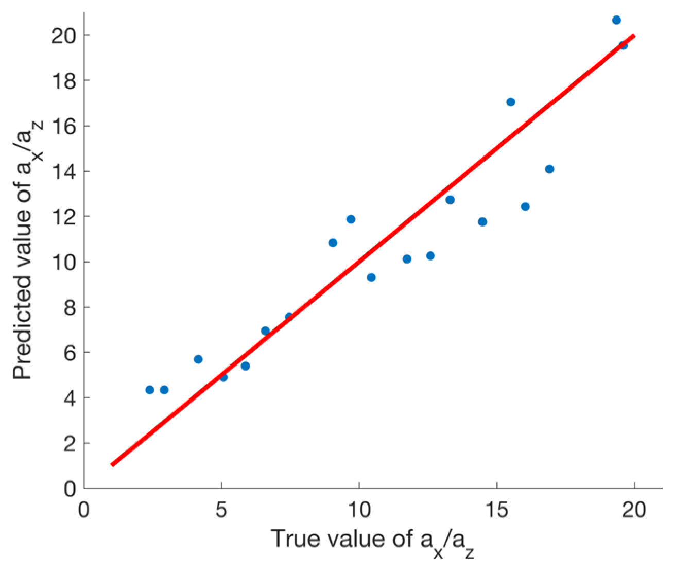
3. Results

3.1. FDTD-Based Synthetic Data

To assess whether and to what extent the trained CNN is capable of estimating the values of $a_x/a_z$ from the 2D GPR autocorrelation images, we first performed tests based on synthetic GPR reflection data, which are generated using a FDTD solution of Maxwell’s equations. It is important to note that data generated in this manner comprehensively account for the physics governing high-frequency electromagnetic wave propagation. As such, they represent the complete GPR wavefield, which, in addition to the primary reflections accounted for by the convolution-based approximation, may comprise multiple reflections and diffractions. To this end, we first generate 20 stochastic subsurface models (Figure 3) with randomly selected values of $a_x$, $a_z$, and $v$. We then simulated the corresponding GPR data using the FDTD algorithm of Irving and Knight [39]. For each simulation, the transmitter and receiver antennas were considered to be spaced 1 m apart and moved with a lateral increment of 0.1 m along the survey profile. The transmitter antenna current function was specified to be the first derivative of a Blackman–Harris window with a dominant frequency of 100 MHz. While the time–history and spectral characteristics of this function are similar to those of the Ricker wavelet used to create the training database, they are importantly not identical, which emulates corresponding discrepancies when applying the trained network to observed GPR data.

The resulting synthetic GPR data were contaminated with zero–mean Gaussian random noise having a standard deviation of 2% with regard to the maximum absolute signal amplitude below the direct wave, and were then subjected to a standard processing sequence involving the following: (i) elimination of the direct air and ground wave arrivals by removing the mean trace computed over a sliding window; (ii) 30–300 MHz bandpass filtering; (iii) amplitude scaling to compensate for the geometric spreading of energy along with scattering and transmission losses using a smooth gain function based on the mean absolute amplitude curve for the whole section; (iv) 2D F-K migration using a constant velocity of 0.1 m/ns, which was found to optimally focus diffraction events; and (v) depth-conversion with a constant velocity of 0.1 m/ns. Figure 4 shows the processed FDTD-simulated GPR data.

We then compute the corresponding 20 autocorrelation images and submit them to the trained CNN to infer the geostatistical parameters of the underlying subsurface models. Figure 5 shows the estimated versus true values of the structural aspect ratio $a_x/a_z$. Overall, the estimations are remarkably accurate and closely follow the 45-degree trend line, which finds its expression in a rather high correlation coefficient of 0.93. The root mean square error (RMSE) is 1.93, further demonstrating the reliability of the predictions. This result is consistent with previous studies demonstrating that the autocorrelation of GPR reflection images is inherently sensitive to the aspect ratio $a_x/a_z$ of the underlying heterogeneity [6,7]. Most importantly, however, it clearly underscores the potential of the novel estimation approach proposed in this study.

3.2. Sensitivity to Noise

To test the sensitivity of the proposed method to the level of noise in the GPR data, we consider the stochastic model presented in Figure 2a, which was not included in the training database, and generate corresponding synthetic data using the FDTD method [39]. The synthetic data are then contaminated with gradually increasing amounts of zero-mean Gaussian random noise before being subjected to the same signal processing flow used in the previous test. In each case, the noise level is set relative to the maximum absolute signal amplitude below the direct arrivals.

Figure 6a,b show the resulting GPR images for noise levels of 2% and 50%, respectively. Comparing Figure 6a and Figure 2a, we observe that the FDTD-based GPR image exhibits a remarkably strong resemblance to its convolution-based counterpart, which importantly corroborates the validity of using the latter type of approximate synthetic data for training the CNN. Although the GPR image shown in Figure 6b retains a clear similarity to its low-noise counterpart (Figure 6a), it is contaminated by a large number of “smiles”, which typically arise when migrating pure random noise or very noisy data [40].

Figure 7 shows the inferred values for $a_x/a_z$ as a function of the noise level. Quite interestingly, these results demonstrate that the estimated values remain remarkably stable even in the presence of significant noise. We observed that the values of $a_x/a_z$ gradually decreased with increasing noise, which is expected due to the decreasing lateral coherence of the GPR reflection images and the corresponding reduction in the lateral autocorrelation length. In this regard, it is important to note that the estimates of $a_x/a_z$ progressively approach their target value with increasing noise content. This is due to the fact that, for the underlying data, our method overestimates the aspect ratio by ~10% at low noise levels (Figure 5 and Figure 7).

3.3. Differences in Spectral Characteristics of Analyzed Data and Training Database

The synthetic GPR data used to train the CNN have a dominant frequency of 100 MHz and, hence, it is implicitly assumed that the spectral characteristics of the analyzed data are similar. For field GPR data, however, this is not guaranteed as, depending on near-surface electrical properties, the dominant frequencies often differ substantially from the corresponding nominal values of the transmitter antennae. To explore the impact of such differences, we again used 20 stochastic models shown in Figure 3 and simulated FDTD-based GPR data having a dominant frequency of 70 MHz. All other simulation parameters are kept unchanged. The resulting GPR reflection data were again contaminated with 2% Gaussian random noise and subjected to the same processing as the 100 MHz data (Figure 8). We then applied the following procedure to compensate for the differences in the spectral characteristics with regard to the training data: (i) calculate the Fourier transform of each trace; (ii) shift the amplitude spectrum upwards by 30 MHz by padding with the appropriate number of zeros; and (iii) transform the shifted spectrum back to the time domain retaining the original phase information. The original and shifted average amplitude spectra are shown in Figure 9.

The 2D autocorrelation images of the GPR data before and after spectral shifting were submitted to the CNN trained on the original 100 MHz database. Figure 10 summarizes the resulting estimations of the structural aspect ratio $a_x/a_z$. The predicted values for the 70 MHz data show a systematic bias towards too low values (Figure 10a), whereas the estimates for the spectrally adjusted data (Figure 10b) agree as well with their target values as those for original 100 MHz FDTD-based synthetic GPR images (Figure 5). The correlation coefficient is 0.95, and the root mean squared error is 2.29. This indicates that the simple spectral adjustment procedure outlined above is a viable tool to compensate for differences in the spectral characteristics of the observed data with regard to the training database. In this context, it is important to note that most commercial GPR systems employ a limited number of “standard” antenna frequencies, for which the spectral bandwidth of the recorded data is quite uniformly in the range of 2 to 3 octaves. We therefore expect that the global training effort of the CNN can be restricted to these nominal values.

3.4. Application to Field Data

Following the preceding tests of our proposed methodology on FDTD-based synthetic data, we now consider its application to common-offset GPR reflection data acquired at the Boise Hydrogeophysical Research Site (BHRS), which is located on a gravel bar adjacent to the Boise River near Boise, Idaho, USA [41]. The surficial, unconfined alluvial aquifer at the BHRS is bound by a clay layer at approximately 20 m depth. The depth to the groundwater table varies seasonally between 0 and 3 m. Over the past two decades, a wide variety of geophysical and hydrogeological studies have been conducted at this site for characterizing heterogeneous alluvial aquifers [13,33,42,43,44]. The considered GPR reflection profile is part of a legacy 3D survey, which was performed in 1998 using a PulseEkko Pro 100 system (Sensors & Software, Inc., Mississauga, ON, Canada) with a nominal antenna center frequency of 100 MHz. The data were collected in common-offset mode using a transmitter–receiver antenna spacing of 1 m. Traces were recorded every 0.2 m along 18 m long profiles. The time sampling interval was 0.8 ns and 32 vertical stacks were performed for each recorded GPR trace to enhance the signal-to-noise ratio. As outlined earlier, second-order geostatistical characterizations should be confined to distinct lithologies and/or hydraulic units to be realistic and representative [9]. In the following, we therefore limit our analysis to the water-saturated zone and remove the top 40 ns comprising the vadose zone.

The considered GPR reflection data were subjected to a processing flow similar to their synthetic counterparts involving time-zero correction, dewow filtering, elimination of direct air and ground waves, 30–300 MHz bandpass filtering, smooth time-varying amplitude gain, and 2D F-K migration and depth conversion using a constant velocity of 0.08 m/ns. This velocity was found to optimally focus diffraction events below the water table and is consistent with the corresponding average value for the saturated zone at the BHRS as determined by Bradford et al. [43]. Figure 11a shows the processed GPR image. The somewhat jagged nature of the amplitude spectrum of the observed GPR data (Figure 11c) renders the estimation of the dominant frequency less straightforward than in the case of the synthetic data (Figure 9). Unlike in the synthetic case, where the center frequency is known, we must estimate the center frequency for the field data. One possibility we explored is to assess the average centroid frequency of the observed data and to use the corresponding difference with the training database to estimate the required spectral shift. Another possibility we considered is to estimate the dominant frequency of the observed data using a half-width-type approach, that is, to determine the mid-point of the amplitude spectrum at approximately half its maximum value. For the considered GPR data, both of these approaches yield an estimated central frequency of ~80 MHz. To make the spectrum of the observed data consistent with that of the training database, we therefore adjusted the former, as outlined above, by an upwards shift of 20 MHz. The comparison of the original and spectrally shifted data in Figure 11a,b is interesting and indicates that this procedure does not introduce any artifacts or otherwise alter the character of the original data apart from rendering them considerably crisper. Clearly, additional options for stabilizing the estimate of the dominant data frequency exist, such as, for example, spectral smoothing, which we have not explored given the simplicity and robustness of the considered approaches.

The autocorrelation image of the spectrally adjusted section was then submitted to the trained CNN, which yields an estimated aspect ratio $a_x/a_z$ of 9.25. For comparison, we also used the original Monte Carlo inversion approach to estimate the aspect ratio for the corresponding original, that is, spectrally not adjusted, processed GPR data [6,7]. The prior range of acceptable values for the horizontal and vertical correlation lengths was set between 0.1 and 3 m. The Monte Carlo estimation was run until 4000 accepted sets of model parameters were obtained. The resulting histogram for the horizontal-to-vertical aspect ratio of the underlying heterogeneity is shown in Figure 12. The corresponding values for the mean and standard deviation are 8.92 and 1.03, respectively, which implies that the value estimated with the newly proposed CNN-based technique is fully consistent with the range of estimates provided by the well-established Monte Carlo approach.

4. Discussion

Our tests on synthetic data illustrate that discrepancies between the dominant frequency of the training database and that of the analyzed GPR data may lead to biased estimates of the structural aspect ratio a_x/a_z. For the specific scenario we considered, where the dominant frequency of the analyzed GPR data was 30% lower than that used to generate the training database, our results indicate that a_x/a_z can be underestimated by up to 50%. Given that discrepancies of this magnitude between the nominal and actually recorded center frequencies are quite typical for commonly used GPR acquisition systems, a careful analysis of the average data amplitude spectrum followed, if necessary, by corresponding adjustments is essential. While our results indicate that the latter can be effectively achieved through a simple spectral shift, more sophisticated approaches such as shaping filters [45] are also conceivable. For larger discrepancies between the center frequencies of the analyzed and training data, it may be advisable to retrain the CNN on a correspondingly targeted database. As typical GPR antenna systems for geological applications tend to be available roughly in octave-type increments of the nominal center frequency (e.g., 50, 100, and 200 MHz), the generation of a widely applicable suite of trained CNNs is straightforward. Finally, the results of our method might also be biased, albeit probably to a lesser extent, by pronounced differences in the spectral bandwidth between the observed and training GPR data. We have not explored this possibility because the spectral bandwidth of approximately two to three octaves, which we used to create our training database, is indeed quite typical for the most commercially available GPR acquisition systems.

Biased estimates of the structural aspect ratio a_x/a_z could also arise when the processed and migrated GPR data are converted to depth with an incorrect average subsurface velocity. In the absence of complementary velocity measurements, such as common-mid-point (CMP) gathers, the most obvious way to estimate the average subsurface velocity from common-offset GPR reflection data is through migration focusing analysis [46]. The inferred velocities do, however, have a tendency to be too low, as artifacts resulting from the use of too high migration velocities are visually more obvious than imperfect focusing of diffracted and/or scattered wavefield components due to the use of too low migration velocities. Our experience indicates that the corresponding underestimation of the average velocity may amount up to 10 to 20%, which results in a bias of comparable magnitude in the estimated structural aspect ratio a_x/a_z. In this context, it is, however, important to note that corresponding estimations of a_x/a_z of based on the classical Monte Carlo approach would be subject to the same kind of bias.

Following the original work of Irving et al. [6], our proposed methodology is based on the analysis of the autocorrelation of the GPR image. This second-order approach provides a clear and simple relationship between the input and the output of the CNN and is generally regarded to be valid for distinct lithological and/or hydraulic units. However, it also results in an inherent loss of valuable information, such as, for example, the phase characteristics of the GPR data. Future work should therefore explore the use of additional inputs for training the CNN, such as the original GPR image as well as one or several versions enhanced by suitable attributes that are sensitive to the structural, lithological, and/or petrophysical characteristics [47]. Another inherent assumption of our approach is that the principal axes of the heterogeneity ellipsoid are aligned with the cardinal directions used to process and display the data. Although there is a prevalence of sub-horizontal stratification in surficial environments [48], this is clearly not ubiquitously adequate. As illustrated by Xu et al. [8], notable deviations from the assumption of horizontal stratification can be readily accounted for through a corresponding coordinate transformation.

As with all deep learning applications in geophysics, the fundamental question arises as to whether the corresponding results, whose inference is devoid of a solid theoretical foundation, are universally valid and trustworthy [17]. This question could at least be partly addressed by estimating the uncertainties of the inferred results, which, in our case, would also allow for a more direct and more comprehensive comparison with the corresponding results inferred through the traditional Monte-Carlo approach. Recent work of this kind, which we expect to explore in our future research efforts, indicates that this can be achieved by utilizing probability distribution as the output target [49].

While the acquisition of surface-based common-offset GPR reflection data along 2D profiles is common, there is a growing tendency towards acquiring surveys in 3D and, correspondingly, the geostatistical analysis of such 3D data will become increasingly important in the future [43]. While, as illustrated by Xu et al. [8], the traditional Monte-Carlo-type inversion approach can be readily adapted and applied to 3D GPR reflection volumes, the associated computational costs are extremely high. In this regard, we expect the proposed CNN-based technique to offer a decisive practical advantage. We anticipate that, for such an extension from 2D to 3D, the size of the training database will likely need to be increased by one to two orders of magnitude, which, in turn, is expected to increase the time required for training the CNN by one to two orders of magnitude or more. Conversely, the generation of the synthetic 3D GPR database for training the CNN remains computationally feasible due to the fact that it can be achieved using the highly efficient convolution approximation. As in the 2D case considered in this work, the application of the trained CNN to observed 3D GPR data is expected to come at virtually no extra computational cost. In view of this, we anticipate that the most important technical challenge for the extension of the proposed technique from 2D to 3D is related to the high computational cost of generating an adequate number of 3D FDTD-based synthetic GPR reflection surveys for testing and benchmarking purposes.

5. Conclusions

In this study, we have presented a novel method for inferring the structural aspect ratio a_x/a_z of subsurface heterogeneity from 2D surface-based GPR reflection images based on supervised deep learning. This approach provides a simple and efficient alternative to the current Monte-Carlo-based inversion of GPR reflection data for this pertinent geostatistical parameter. The proposed method utilizes a CNN trained on a large database of autocorrelations derived from synthetic GPR reflection images. This synthetic training database is generated for a wide range of stochastic subsurface models using a computationally efficient but approximate convolution-based modeling algorithm. The effectiveness of our approach is assessed and validated using realistic FDTD-based synthetic common-offset GPR reflection data as well as field data. Our results also demonstrate that the proposed method is robust to the presence of noise and that typical differences with regard to the dominant frequencies between the analyzed GPR data and the synthetic database used to train the CNN can be readily accommodated through simple spectral shifting operations. Compared to the traditional Monte Carlo inversion approach, the considered CNN-based technique offers significant enhancements in computational efficiency, requiring only minimal additional overhead after training. The latter is expected to become particularly advantageous for an eventual extension of this technique to 3D, which is conceptually straightforward and practically feasible due to the fact that the synthetic training database can be generated through a computationally highly efficient approximate modeling approach. Although this study focuses on GPR reflection data, previous related experience with the traditional Monte-Carlo-based inversion approach indicates that the newly proposed methodology should also be readily applicable to seismic reflection data.

References

- Rea, J.; Knight, R. Geostatistical analysis of ground-penetrating radar data: A means of describing spatial variation in the subsurface. Water Resour. Res. 1998, 34, 329–339. [Google Scholar] [CrossRef]
- Dafflon, B.; Tronicke, J.; Holliger, K. Inferring the lateral subsurface correlation structure from georadar data: Methodological background and experimental evidence. In Geostatistics for Environmental Applications; Springer: Berlin/Heidelberg, Germany, 2005; pp. 467–478. [Google Scholar]
- Knight, R.J.; Irving, J.D.; Tercier, P.; Freeman, G.J.; Murray, C.J.; Rockhold, M.L. A comparison of the use of radar images and neutron probe data to determine the horizontal correlation length of water content. Subsurf. Hydrol. Data Integr. Prop. Process. 2007, 171, 31–44. [Google Scholar]
- Knight, R.; Tercier, P.; Irving, J. The effect of vertical measurement resolution on the correlation structure of a ground penetrating radar reflection image. Geophys. Res. Lett. 2004, 31, 2–5. [Google Scholar] [CrossRef]
- Oldenborger, G.A.; Knoll, M.D.; Barrash, W. Effects of signal processing and antenna frequency on the geostatistical structure of ground-penetrating radar data. J. Environ. Eng. Geophys. 2004, 9, 201–212. [Google Scholar] [CrossRef]
- Irving, J.; Knight, R.; Holliger, K. Estimation of the lateral correlation structure of subsurface water content from surface-based ground-penetrating radar reflection images. Water Resour. Res. 2009, 45, W12404. [Google Scholar] [CrossRef]
- Irving, J.; Holliger, K. Geostatistical inversion of seismic and ground-penetrating radar reflection images: What can we actually resolve? Geophys. Res. Lett. 2010, 37, L21306. [Google Scholar] [CrossRef]
- Xu, Z.; Irving, J.; Lindsay, K.; Bradford, J.; Zhu, P.; Holliger, K. Estimation of the 3D correlation structure of an alluvial aquifer from surface-based multi-frequency ground-penetrating radar reflection data. Geophys. Prospect. 2020, 68, 678–689. [Google Scholar] [CrossRef]
- Xu, Z.; Irving, J.; Liu, Y.; Zhu, P.; Holliger, K. Conditional stochastic inversion of common-offset ground-penetrating radar reflection data. Geophysics 2021, 86, WB89–WB99. [Google Scholar] [CrossRef]
- Scholer, M.; Irving, J.; Holliger, K. Estimation of the correlation structure of crustal velocity heterogeneity from seismic reflection data. Geophys. J. Int. 2010, 183, 1408–1428. [Google Scholar] [CrossRef]
- Liu, Y.; Greenwood, A.; Hetényi, G.; Baron, L.; Holliger, K. High-resolution seismic reflection survey crossing the Insubric Line into the Ivrea-Verbano Zone: Novel approaches for interpreting the seismic response of steeply dipping structures. Tectonophysics 2021, 816, 229035. [Google Scholar] [CrossRef]
- Dafflon, B.; Irving, J.; Holliger, K. Use of high-resolution geophysical data to characterize heterogeneous aquifers: Influence of data integration method on hydrological predictions. Water Resour. Res. 2009, 45, W09413. [Google Scholar] [CrossRef]
- Liu, Y.; Irving, J.; Holliger, K. High-resolution velocity estimation from surface-based common-offset GPR reflection data. Geophys. J. Int. 2022, 230, 131–144. [Google Scholar] [CrossRef]
- LeCun, Y.; Bengio, Y.; Hinton, G. Deep learning. Nature 2015, 521, 436–444. [Google Scholar] [CrossRef]
- Goodfellow, I.; Bengio, Y.; Courville, A. Deep Learning; MIT Press: Cambridge, MA, USA, 2016. [Google Scholar]
- Dramsch, J.S. 70 years of machine learning in geoscience in review. Adv. Geophys. 2020, 61, 1–55. [Google Scholar]
- Yu, S.; Ma, J. Deep learning for geophysics: Current and future trends. Rev. Geophys. 2021, 59, e2021RG000742. [Google Scholar] [CrossRef]
- Mousavi, S.M.; Beroza, G.C. Deep-learning seismology. Science 2022, 377, eabm4470. [Google Scholar] [CrossRef]
- Zhu, W.; Mousavi, S.M.; Beroza, G.C. Seismic signal denoising and decomposition using deep neural networks. IEEE Trans. Geosci. Remote Sens. 2019, 57, 9476–9488. [Google Scholar] [CrossRef]
- Kaur, H.; Pham, N.; Fomel, S. Improving the resolution of migrated images by approximating the inverse Hessian using deep learning. Geophysics 2020, 85, WA173–WA183. [Google Scholar] [CrossRef]
- Yang, L.; Chen, W.; Wang, H.; Chen, Y. Deep learning seismic random noise attenuation via improved residual convolutional neural network. IEEE Trans. Geosci. Remote Sens. 2021, 59, 7968–7981. [Google Scholar] [CrossRef]
- Wu, X.; Liang, L.; Shi, Y.; Fomel, S. FaultSeg3D: Using synthetic data sets to train an end-to-end convolutional neural network for 3D seismic fault segmentation. Geophysics 2019, 84, IM35–IM45. [Google Scholar] [CrossRef]
- Song, S.; Mukerji, T.; Hou, J. Bridging the Gap between Geophysics and Geology with Generative Adversarial Networks. IEEE Trans. Geosci. Remote Sens. 2022, 60, 5902411. [Google Scholar] [CrossRef]
- Yang, F.; Ma, J. Deep-learning inversion: A next-generation seismic velocity model building method. Geophysics 2019, 84, R583–R599. [Google Scholar] [CrossRef]
- Di, H.; Abubakar, A. Estimating subsurface properties using a semi-supervised neural networks approach. Geophysics 2021, 87, IM1–IM10. [Google Scholar] [CrossRef]
- Geng, Z.; Zhao, Z.; Shi, Y.; Wu, X.; Fomel, S.; Sen, M. Deep learning for velocity model building with common-image gather volumes. Geophys. J. Int. 2022, 228, 1054–1070. [Google Scholar] [CrossRef]
- Schmelzbach, C.; Tronicke, J.; Dietrich, P. High-resolution water content estimation from surface-based ground-penetrating radar reflection data by impedance inversion. Water Resour. Res. 2012, 48, W08505. [Google Scholar] [CrossRef]
- Pullammanappallil, S.; Levander, A.; Larkin, S.P. Estimation of crustal stochastic parameters from seismic exploration data. J. Geophys. Res. Solid Earth 1997, 102, 15269–15286. [Google Scholar] [CrossRef]
- Poppeliers, C. Estimating vertical stochastic scale parameters from seismic reflection data: Deconvolution with non-white reflectivity. Geophys. J. Int. 2007, 168, 769–778. [Google Scholar] [CrossRef]
- Goff, J.A.; Jordan, T.H. Stochastic modeling of seafloor morphology: Inversion of sea beam data for second-order statistics. J. Geophys. Res. Solid Earth 1988, 93, 13589–13608. [Google Scholar] [CrossRef]
- Tronicke, J.; Holliger, K. Quantitative integration of hydrogeophysical data: Conditional geostatistical simulation for characterizing heterogeneous alluvial aquifers. Geophysics 2005, 70, H1–H10. [Google Scholar] [CrossRef]
- Holliger, K.; Levander, A.R.; Goff, J.A. Stochastic modeling of the reflective lower crust: Petrophysical and geological evidence from the Ivera Zone (northern Italy). J. Geophys. Res. Solid Earth 1993, 98, 11967–11980. [Google Scholar] [CrossRef]
- Tronicke, J.; Holliger, K.; Barrash, W.; Knoll, M.D. Multivariate analysis of cross-hole georadar velocity and attenuation tomograms for aquifer zonation. Water Resour. Res. 2004, 40, W01519. [Google Scholar] [CrossRef]
- LeCun, Y.; Bottou, L.; Bengio, Y.; Haffner, P. Gradient-based learning applied to document recognition. Proc. IEEE 1998, 86, 2278–2324. [Google Scholar] [CrossRef]
- Krizhevsky, A.; Sutskever, I.; Hinton, G.E. Imagenet classification with deep convolutional neural networks. Adv. Neural Inf. Process. Syst. 2012, 25, 1–9. [Google Scholar] [CrossRef]
- Qian, N. On the momentum term in gradient descent learning algorithms. Neural Netw. 1999, 12, 145–151. [Google Scholar] [CrossRef]
- Bottou, L.; Curtis, F.E.; Nocedal, J. Optimization methods for large-scale machine learning. SIAM Rev. 2018, 60, 223–311. [Google Scholar] [CrossRef]
- Smith, L.N. Cyclical learning rates for training neural networks. In Proceedings of the 2017 IEEE Winter Conference on Applications of Computer Vision (WACV), Santa Rosa, CA, USA, 24–31 March 2017; pp. 464–472. [Google Scholar]
- Irving, J.; Knight, R. Numerical modeling of ground-penetrating radar in 2-D using MATLAB. Comput. Geosci. 2006, 32, 1247–1258. [Google Scholar] [CrossRef]
- Yilmaz, Ö. Seismic Data Analysis: Processing, Inversion, and Interpretation of Seismic Data; Society of Exploration Geophysicists: Tulsa, OK, USA, 2001. [Google Scholar]
- Barrash, W.; Clemo, T. Hierarchical geostatistics and multifacies systems: Boise Hydrogeophysical Research Site, Boise, Idaho. Water Resour. Res. 2002, 38, 14-1–14-18. [Google Scholar] [CrossRef]
- Dafflon, B.; Barrash, W. Three-dimensional stochastic estimation of porosity distribution: Benefits of using ground-penetrating radar velocity tomograms in simulated-annealing- based or Bayesian sequential simulation approaches. Water Resour. Res. 2012, 48, W05553. [Google Scholar] [CrossRef]
- Bradford, J.H.; Clement, W.P.; Barrash, W. Estimating porosity with ground-penetrating radar reflection tomography: A controlled 3-D experiment at the Boise Hydrogeophysical Research Site. Water Resour. Res. 2009, 45, W00D26-1–W00D26-11. [Google Scholar] [CrossRef]
- Pirot, G.; Linde, N.; Mariethoz, G.; Bradford, J.H. Probabilistic inversion with graph cuts: Application to the Boise Hydrogeophysical Research Site. Water Resour. Res. 2017, 53, 1231–1250. [Google Scholar] [CrossRef]
- van der Baan, M. Time-varying wavelet estimation and deconvolution by kurtosis maximization. Geophysics 2008, 73, 11–18. [Google Scholar] [CrossRef]
- Liu, Y.; Irving, J.; Holliger, K. Weighted Diffraction-Based Migration Velocity Analysis of Common-Offset GPR Reflection Data. IEEE Trans. Geosci. Remote Sens. 2023, 61, 5901509. [Google Scholar] [CrossRef]
- Lowney, B.; Lokmer, I.; O’Brien, G.S. Multi-domain diffraction identification: A supervised deep learning technique for seismic diffraction classification. Comput. Geosci. 2021, 155, 104845. [Google Scholar] [CrossRef]
- Gelhar, L.W. Stochastic Subsurface Hydrology; Prentice-Hall: Englewood Cliffs, NJ, USA, 1993. [Google Scholar]
- Grana, D.; Azevedo, L.; Liu, M. A comparison of deep machine learning and Monte Carlo methods for facies classification from seismic data. Geophysics 2020, 85, WA41–WA52. [Google Scholar] [CrossRef]
Disclaimer/Publisher’s Note: The statements, opinions and data contained in all publications are solely those of the individual author(s) and contributor(s) and not of MDPI and/or the editor(s). MDPI and/or the editor(s) disclaim responsibility for any injury to people or property resulting from any ideas, methods, instructions or products referred to in the content. |
© 2025 by the authors. Licensee MDPI, Basel, Switzerland. This article is an open access article distributed under the terms and conditions of the Creative Commons Attribution (CC BY) license (https://creativecommons.org/licenses/by/4.0/).
Share and Cite
Liu, Y.; Irving, J.; Holliger, K. Estimating Subsurface Geostatistical Properties from GPR Reflection Data Using a Supervised Deep Learning Approach. Remote Sens. 2025, 17, 2284. https://doi.org/10.3390/rs17132284
Liu Y, Irving J, Holliger K. Estimating Subsurface Geostatistical Properties from GPR Reflection Data Using a Supervised Deep Learning Approach. Remote Sensing. 2025; 17(13):2284. https://doi.org/10.3390/rs17132284
Chicago/Turabian StyleLiu, Yu, James Irving, and Klaus Holliger. 2025. "Estimating Subsurface Geostatistical Properties from GPR Reflection Data Using a Supervised Deep Learning Approach" Remote Sensing 17, no. 13: 2284. https://doi.org/10.3390/rs17132284
APA StyleLiu, Y., Irving, J., & Holliger, K. (2025). Estimating Subsurface Geostatistical Properties from GPR Reflection Data Using a Supervised Deep Learning Approach. Remote Sensing, 17(13), 2284. https://doi.org/10.3390/rs17132284