Article

MCRS-YOLO: Multi-Aggregation Cross-Scale Feature Fusion Object Detector for Remote Sensing Images

School of Automation, Nanjing University of Science and Technology, Nanjing 210094, China
*
Author to whom correspondence should be addressed.
Remote Sens. 2025, 17(13), 2204; https://doi.org/10.3390/rs17132204
Submission received: 8 May 2025 / Revised: 20 June 2025 / Accepted: 23 June 2025 / Published: 26 June 2025

Abstract

With the rapid development of deep learning, object detection in remote sensing images has attracted extensive attention. However, remote sensing images typically exhibit the following characteristics: significant variations in object scales, dense small targets, and complex backgrounds. To address these challenges, a novel object detection method named MCRS-YOLO is innovatively proposed. Firstly, a Multi-Branch Aggregation (MBA) network is designed to enhance information flow and mitigate challenges caused by insufficient object feature representation. Secondly, we construct a Multi-scale Feature Refinement and Fusion Pyramid Network (MFRFPN) to effectively integrate spatially multi-scale features, thereby augmenting the semantic information of feature maps. Thirdly, a Large Depth-wise Separable Kernel (LDSK) module is proposed to comprehensively capture contextual information while achieving an enlarged effective receptive field. Finally, the Normalized Wasserstein Distance (NWD) is introduced into hybrid loss training to emphasize small object features and suppress background interference. The efficacy and superiority of MCRS-YOLO are rigorously validated through extensive experiments on two publicly available datasets: NWPU VHR-10 and VEDAI. Compared with the baseline YOLOv11, the proposed method demonstrates improvements of 4.0% and 6.7% in mean Average Precision (mAP), which provides an efficient and accurate solution for object detection in remote sensing images.

1. Introduction

Driven by rapid technological advancements, the remote sensing imagery domain is undergoing unprecedented growth, demonstrating remarkable progress across multiple dimensions [1,2,3]. Remote sensing is closely connected to disciplines such as geomatics and surveying technology, computer science, earth sciences, and optoelectronic information. It is widely applied in military intelligence [4], urban planning [5], resource exploration [6], and other areas. Furthermore, object detection in remote sensing imagery is now an indispensable technology, drawing widespread interest from multiple fields. Object detection aims to identify specific targets within visual data while precisely localizing their spatial coordinates and semantic categories, enabling efficient extraction of actionable intelligence through localized region-of-interest analysis [7,8,9].
Deep-learning-based approaches for remote sensing object detection are broadly categorized into single-stage and two-stage architectures. Single-stage object detection algorithms do not explicitly generate regions of interest (ROIs) but instead formulate the detection task as a unified regression problem applied to the entire image. Representative single-stage detection algorithms include Single Shot MultiBox Detector (SSD) [10], You Only Look Once (YOLO) [11], and CenterNet [12]. In contrast, two-stage frameworks decompose the task into sequential phases: region proposal generation and target classification with localization. In the first phase, a Region Proposal Network (RPN) or a similar mechanism generate candidate regions by sliding predefined anchor boxes over feature maps, leveraging saliency analysis and spatial likelihood to identify potential target areas. These proposals undergo preliminary classification and bounding box regression. During the second phase, dedicated classification and regression subnetworks—integrated within the convolutional architecture—refine the candidate regions by extracting discriminative features to output precise target categories and spatial coordinates. The R-CNN series, including R-CNN [13], Fast R-CNN [14], Faster R-CNN [15], and Mask R-CNN [16], represents the canonical two-stage detection paradigm. While these methods excel on natural image benchmarks dominated by large objects against uncluttered backgrounds, their direct application to remote sensing imagery faces distinct challenges. The prevalence of small targets, extreme scale variations, and complex spatial contexts necessitates specialized architectural adaptations beyond conventional frameworks optimized for natural imagery.
However, remote sensing imagery presents unique challenges due to extreme variations in imaging altitudes, leading to substantial scale disparities across different object categories. Even for objects within the same category, significant intra-class scale diversity is frequently observed in aerial scenes. This pronounced scale discrepancy imposes severe constraints on feature extraction in convolutional neural networks (CNNs). While deep CNN layers capture contextual information to infer environmental context and coarse object outlines, they inevitably discard localized details critical for characterizing multi-scale targets. Consequently, relying solely on these high-level features fails to comprehensively represent objects with drastic scale variations, often resulting in missed detections that severely impact detection accuracy. These objects exhibit limited pixel coverage, indistinct feature representations, and scarce positive samples. Simultaneously, their precise localization poses substantial challenges as most deep learning architectures struggle to extract discriminative features from such minimal pixel footprints. Progressive down-sampling operations in conventional networks exacerbate this issue, causing progressive degradation of small object features into blurred and indistinguishable representations. Additionally, the structurally complex backgrounds of remote sensing images—containing redundant non-target objects with visual similarities to true targets—frequently induce false positives. This complexity also hinders precise edge feature extraction from imagery and complicates foreground–background separation, presenting a significant obstacle for reliable detection systems.
To address these challenges, we innovatively propose the MCRS-YOLO network for object detection in remote sensing images. This paper introduces a detection model based on YOLOv11 [17], which enhances information flow and reduces object information loss through a multi-branch aggregation network. By reconstructing the feature pyramid via dynamic interpolation and multi-feature fusion, the model’s multiscale feature representation capability is further improved, and spatial semantic information is enriched. The introduction of a large depth-wise separable kernel module effectively leverages contextual information, expands the effective receptive field, and enhances detection performance for small objects. Additionally, the integration of NWD [18] improves the model’s ability to recognize targets in complex backgrounds. The experimental results demonstrate that these optimization strategies significantly enhance the performance of object detection in remote sensing images.
The main contributions of this paper are as follows:
  • The MBA is designed in this paper. Multiple convolutional variants such as bypass convolution and depth-wise separable convolution (DSConv) are synergistically integrated into the deeper layers of the backbone network. In the neck network, we further combined convolutional operations with gating mechanisms. This design effectively enhances the diversity of visual features and improves information flow, thereby strengthening the network’s ability to model dense spatial transformations and mitigating the challenges caused by insufficient object information;
  • The MFRFPN is designed for spatial feature reconstruction and multi-scale pyramid context extraction. It captures the global context in both horizontal and vertical directions, obtaining the axial global context to explicitly model rectangular critical regions, effectively integrates hierarchical feature information, and enhances the model’s contextual awareness. Through dynamic interpolation and multi-feature fusion, the network further improves multi-scale feature representation capabilities and strengthens the model’s ability to recognize targets in complex backgrounds;
  • The LDSK is proposed in this paper. This module achieves an expanded effective receptive field by decomposing the 2D kernels of depth-wise convolution and dilated depth-wise convolution into two cascaded 1D separable kernels. By integrating multi-scale receptive field information and establishing long-range dependencies, it enhances feature extraction capabilities to improve small object perception;
  • The NWD is introduced into hybrid loss training, where a novel metric is utilized to measure the similarity of bounding boxes. It mitigates the sensitivity of conventional metrics to positional deviations in small objects, enhances the saliency of small target features, and suppresses background noise.
The remainder of this paper is organized as follows: Section 2 reviews related work in the field. Section 3 elaborates on the proposed methodology in detail. 
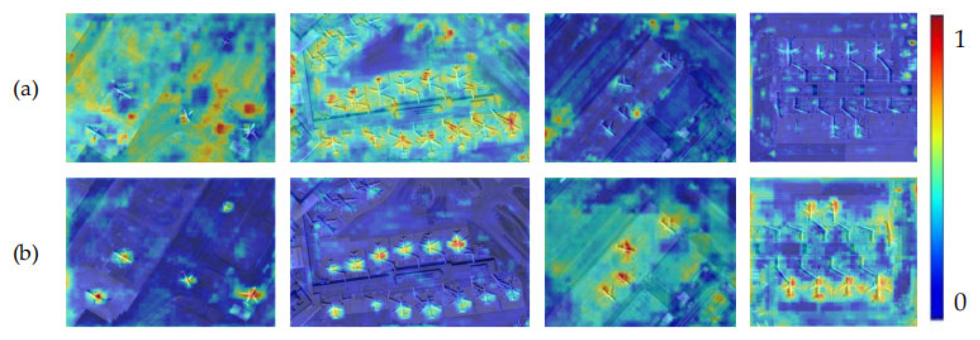
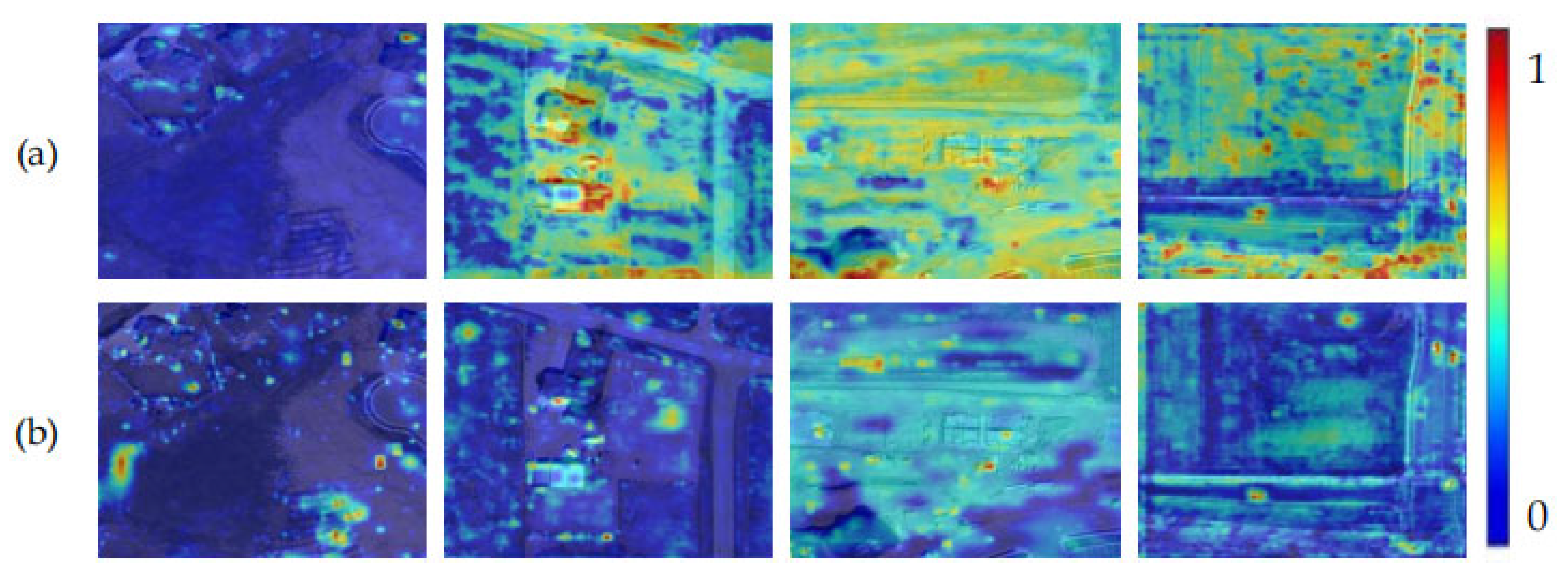
Section 4 evaluates and analyzes the method through ablation studies, comparative experiments, and visualization analyses to validate its efficacy. Finally, Section 5 concludes this study and outlines potential directions for future research.

2. Related Work

2.1. Efficient Convolutional Network

Refinements to convolutional networks enable enhanced capture of detailed target features in remote sensing imagery and improved feature extraction capabilities. Wang et al. [19] introduced SPD Conv to successfully boost detection accuracy for weakly distinguishable targets. Li et al. [20] mitigated information degradation by adopting GhostNetV2 convolution modules. Zheng et al. [21] enhanced the network’s ability through multi-branch convolutional structures and dilated convolutions to extract discriminative semantic information. Li et al. [22] utilized depth-wise separable convolutions, dilated convolutions, and SE layer modules to extract multi-scale information across network stages, improving target detection in complex scenes. The object-specific enhancement methodology introduced in [23] systematically augments discriminative feature representation. Fan et al. [24] leveraged large-kernel depth-wise separable convolutions for capturing global context features, which enhances the detection precision of objects against cluttered background.
However, many algorithms typically focus on solving problems from the perspective of global features, lacking sufficient ability to perceive local details, and failing to fully utilize object information. This results in limited improvement in the model’s capability to detect small targets.

2.2. Feature Pyramid Reconstruction

Reconstructing the feature pyramid enables networks to better adapt to target scale variations while enhancing feature propagation and interaction. Lin et al. [25] pioneered the Feature Pyramid Network (FPN), a landmark architecture that enhances object detection performance by cross-layer feature fusion, leveraging both high-level semantics and low-level spatial details. Subsequently, numerous enhanced FPN variants have been developed, optimizing network architectures and weighting strategies. These advancements include PANet [26], NAS-FPN [27], and BiFPN [28]. Feature fusion was optimized by Jiang et al. [29] via cross-layer multi-scale integration, while Li et al. [30] implemented BiFPN with top–down and bottom–up pathways for efficient feature propagation. Cheng et al. [31] introduced MFANet, a multi-scale aggregation architecture, for improved feature propagation. Jiang et al. [32] developed the Multi-scale Feature Context Aggregation Network (MFCANet), aggregating and fusing contextual information across feature maps of varying scales to improve detection capability.
However, existing feature pyramid construction methods still face issues such as imbalanced feature fusion during cross-scale integration, as well as the overlap of semantic information between different levels. These problems increase the risks of undetected objects and incorrect identifications, thereby degrading the recognition capability for small targets.

2.3. Feature Enhancement Strategy

Feature enhancement enables better focus on critical information while concentrating on essential information more prominently and reducing the influence of unrelated background noise, thereby boosting the performance of object detection in terms of accuracy. Tian et al. [33] designed a Deformable Attention Module that adaptively learns displacement offsets of reference points to prioritize meaningful local features, enhancing the network’s local perception. Yi et al. [34] proposed CloAttention, a dual-branch architecture combining global context modeling via down-sampled attention with local feature enhancement through depth-wise convolutions and gated mechanisms. Zhang et al. [35] enhanced feature learning through a dual-branch architecture resolving spatial–channel interplay constraints, leveraging cross-dimensional attention and residual gating mechanisms. Cheng et al. [36] employed dual spatial–channel attention in advance of feature fusion, markedly strengthening the discriminative power of spatial and semantic cues. Shen et al. [3] applied coordinated attention across distinct feature hierarchies, reinforcing contextual relationships. Li et al. [37] incorporated both self-attention and cross-attention mechanisms to enable robust modeling of object-context correlations.
However, most feature enhancement strategies insufficiently exploit contextual information, failing to effectively capture meaningful contextual dependencies. Furthermore, inter-object relationships in complex scenes are largely neglected, undermining the model’s holistic understanding of intricate scenarios.

3. Methods

Compared to previous versions, YOLOv11 stands out with an enhanced model structure. Its optimized gradient paths and modular design boost feature extraction while keeping the model lightweight. This suits it well for remote sensing images with complex backgrounds and multi-scale targets. YOLOv11 also has lower computational complexity than other YOLO versions. With GPU optimization and architectural improvements, YOLOv11 achieves faster inference speed than other YOLO variants, which is crucial for real-time processing of remote sensing imagery.
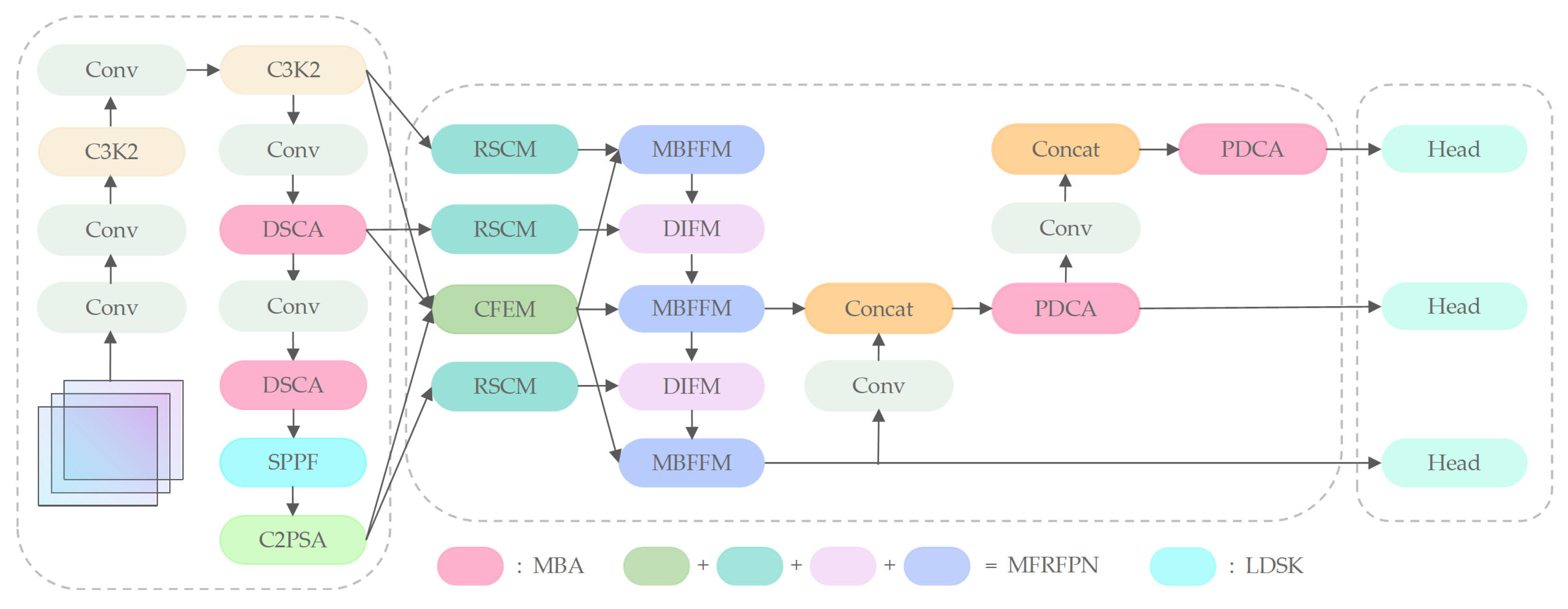
The YOLOv11 architecture comprises three core components: the backbone, neck, and head. The backbone network—incorporating modules like C3K2, SPPF, and C2PSA—serves as the primary feature extractor. In YOLOv11, the C3K2 module extracts features via stacked standard convolutional layers. However, it lacks multi-branch convolutions and local-–lobal feature interaction mechanisms, making it hard to retain fine-grained information of small targets. The SPPF module expands the receptive field through fixed-kernel-size pooling operations, but this leads to insufficient modeling of long-range dependencies for small targets. Additionally, the neck uses a traditional feature pyramid structure without adequately modeling the axial global context; so, it struggles to handle complex spatial relationships in remote sensing images. The loss function in YOLOv11 relies on the traditional IoU metric, which is highly sensitive to positional deviations in small object detection. Boundary box prediction errors for small objects are easily amplified, increasing both false positive and false negative rates. Therefore, we propose MCRS-YOLO, a network architecture specifically optimized for small object detection in remote sensing imagery. The overall framework is illustrated in Figure 1.
Given the diminutive size and limited informational content of small objects, backbone networks struggle to capture their discriminative features. To address this, we propose the Depth-wise Separable Aggregation (DSCA) network in the deeper layers of the backbone, enhancing semantic depth and foundational feature extraction capabilities. Concurrently, we introduce the LDSK within the backbone’s feature extraction pipeline to expand the effective receptive field. The processed features from three distinct scales are then propagated to the neck network. Recognizing the pronounced scale variability of targets in remote sensing imagery, we observe that conventional neck designs inadequately leverage contextual guidance for multi-scale feature fusion, limiting spatial fidelity. The MFRFPN is proposed within the neck to resolve this issue through enhanced spatial feature reconstruction and multi-scale context aggregation. Additionally, the Partial Depth-wise Context Aggregation (PDCA) network is integrated to strengthen global perception of multi-scale targets. These innovations synergistically mitigate information degradation during feature transmission while enriching spatial–semantic representations and enabling more effective cross-scale integration. Further addressing the challenge of spatial sensitivity in small object detection—where complex background interference frequently introduces localization noise—we implement a hybrid loss training strategy that reduces IoU metric sensitivity to positional deviations. This approach suppresses background interference through adaptive weighting of localization confidence and semantic discriminability, ultimately enhancing overall detection robustness.
MBA’s DSCA replaces the C3K2 module in the deep layers of the backbone, and its PDCA is integrated into the neck network. MBA serves as the foundation of the network, providing enhanced features for subsequent modules like MFRFPN, LDSK, and NWD. Its enriched feature diversity improves MFRFPN’s multi-scale feature fusion, offers a stronger basis for LDSK’s context extraction, and aids NWD in accurately measuring bounding box similarity. MFRFPN relies on high-quality features from MBA for multi-scale feature reconstruction and fusion. LDSK’s ability to capture wide-ranging context features complements MFRFPN’s integration of features across scales. MFRFPN’s output is also a key basis for NWD’s bounding box similarity calculations. LDSK expands the receptive field to capture broader context information, working with MFRFPN to provide detailed local features and rich global context. The context features extracted by LDSK also inform NWD’s calculations. NWD optimizes the model’s prediction results based on high-quality features from preceding modules like MBA, MFRFPN, and LDSK. Improvements in these modules enhance NWD’s effectiveness.

3.1. Multi-Branch Aggregation Network

For the purpose of enhancing the diversity of visual characteristics and improve information flow, strengthen the network’s capability in modeling spatial transformations, and mitigate challenges caused by insufficient object feature representation, we propose the MBA. The MBA is not a single monolithic block, but rather a distributed design integrated at two strategic locations within the network architecture. As illustrated in the overall framework of Figure 1 in this paper, the MBA module primarily corresponds to the following two components. The DSCA is embedded deep within the backbone network, aiming to enhance feature extraction capability and semantic depth. The PDCA is integrated into the neck network, designed to strengthen global perception and multi-scale feature fusion. Specifically, DSCA replaces the original C3K2 module in the backbone, while PDCA is incorporated into the neck structure. These two components together constitute the MBA module, which is strategically placed across the core processing pipeline of the detection framework—from the backbone to the neck.

3.1.1. Convolutional Backbone Network

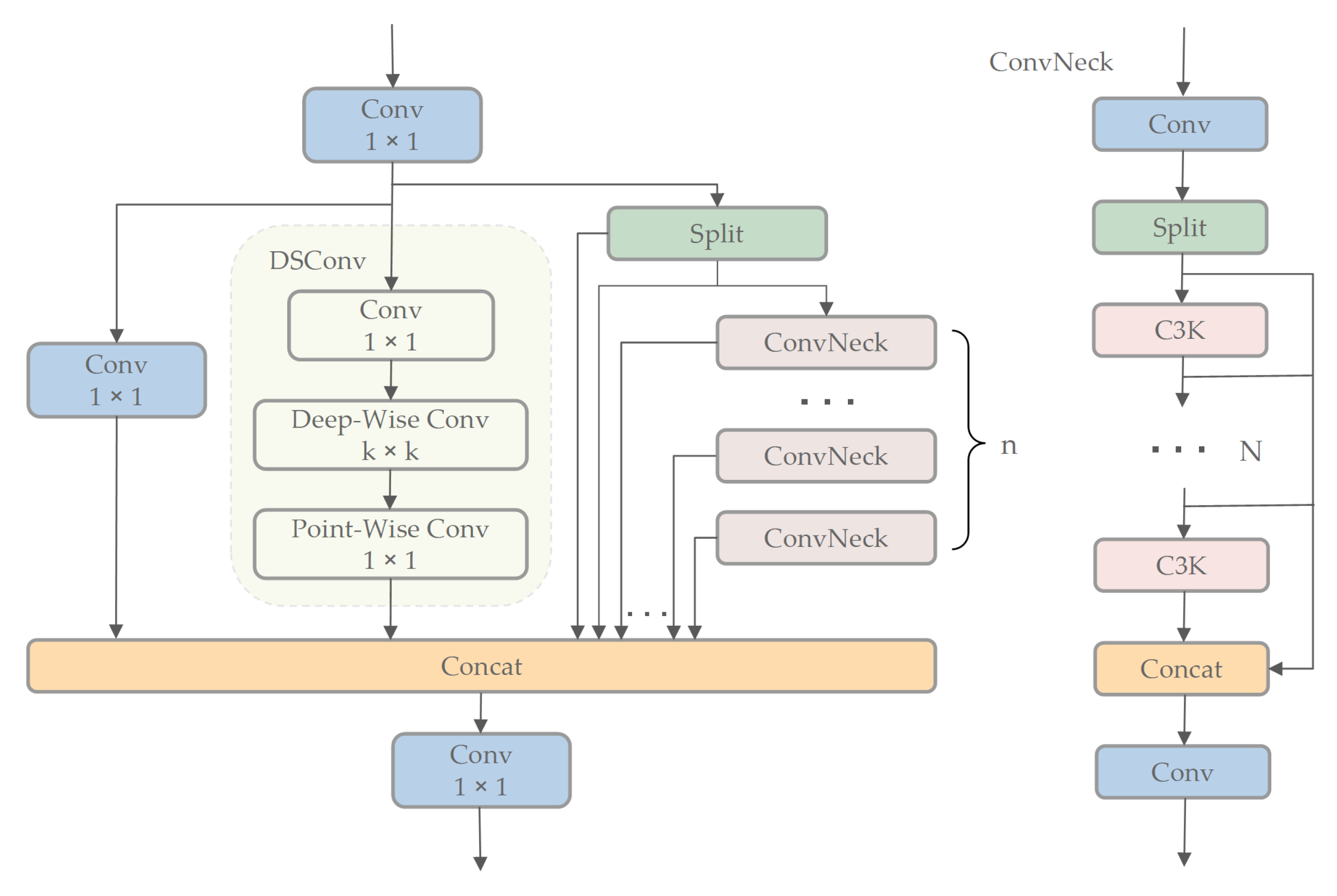
For enhancing the feature extraction performance of the MCRS-YOLO backbone in deeper layers, the DSCA is developed. The objective of DSCA is to synergize diverse convolutional operations—including depth-wise separable convolutions, bypass convolutions, and hierarchical feature recalibration—thereby improving feature discriminability, strengthening gradient propagation, and enhancing multi-level feature representation and semantic depth. The architecture of DSCA is depicted in Figure 2.
DSCA combines three convolutional variants—1 × 1 bypass convolution for channel-wise feature recalibration, DSConv for efficient spatial processing, and the C3K2 module for enhanced hierarchical integration—to improve the information flow. This integration generates a more diverse and enriched gradient flow during training, significantly enhancing the semantic depth of foundational features while effectively enriching contextual information. We apply batch normalization (BN) after each Conv operation in the DSCA module to maintain feature diversity and achieve lower latency. BN can be merged into adjacent Conv layers, stabilizing training and improving inference efficiency. This is crucial for ensuring compatibility among multi-branch convolutional paths and maintaining inter-layer gradient flow. The method BN is applied. A notable advantage of BN is its capability to be incorporated into nearby convolutional layers, leading to improved inference efficiency. The DSCA architecture is formulated as follows:
x m i d = C o n v 1 x i n x 1 = C o n v 2 x m i d x 2 = D S C o n v C o n v 3 ( x m i d ) x 3 , x 4 = S p l i t x m i d x 5 = C o n v N e c k 1 x 4 + x 4 x 6 = C o n v N e c k 2 x 5 + x 5 x 4 + n = C o n v N e c k n x 3 + n + x 3 + n
The channel number of x m i d is 2c. The channel count for x 1   , x 2   , , x 4 + n is c. Finally, we fuse and compress the three features through concatenation, followed by a 1 × 1 convolution to generate the output x o u t with a channel number of 2c, as shown below:
x o u t = C o n v 0 x 1 | | x 2 | | | | x 4 + n

3.1.2. Convolutional Neck Network

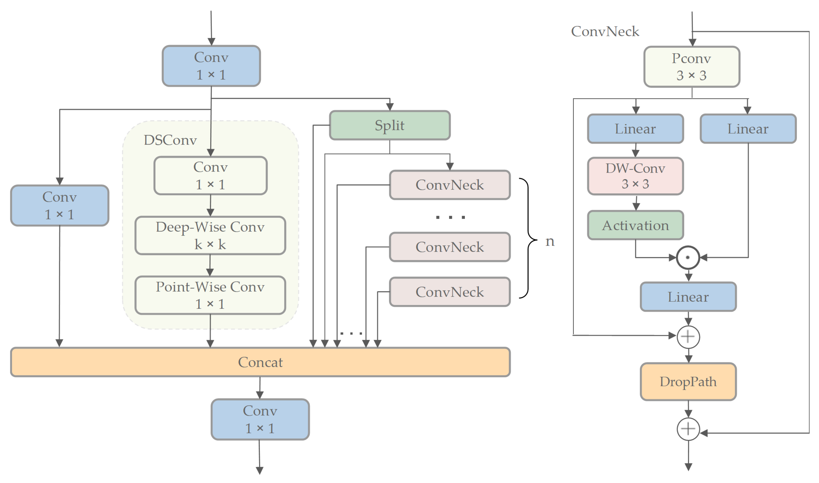
The neck network is typically used to combine feature maps from various hierarchical stages, generating multi-scale feature representations to improve object detection accuracy. To achieve this, we further enhance DSCA and propose PDCA. Specifically, we redesign the ConvNeck component in DSCA by incorporating partial convolutions and depth-wise convolutions.
The ConvNeck in PDCA comprises partial convolution (PConv), depth-wise convolution, linear transformations, activation functions, and regularization operations. The input is processed through PConv, where spatial features are captured by performing standard convolutional operations to a selected channel subset, while others retain their original values without computation. For efficient memory access, contiguous channels at the start or end are selected as computational representatives. The process then splits into dual paths: the left branch sequentially applies linear transformation, depth-wise convolution, and gated activation, while the right branch directly applies linear transformation. The outputs from both branches are merged through element-wise multiplication to enhance discriminative features, with a subsequent linear transformation applied for dimensionality adjustment. The depth-wise convolution implicitly captures positional information from zero-padding, acting as conditional positional encoding. The result is added to the PConv-processed input, regularized via DropPath to maintain information flow and prevent overfitting, and finally merged with the original input via residual addition to generate the fused output. This design leverages depth-wise convolution to refine gating signals using local features, enhancing model performance. The architecture is illustrated in Figure 3.

3.2. Reconstructed Feature Pyramid

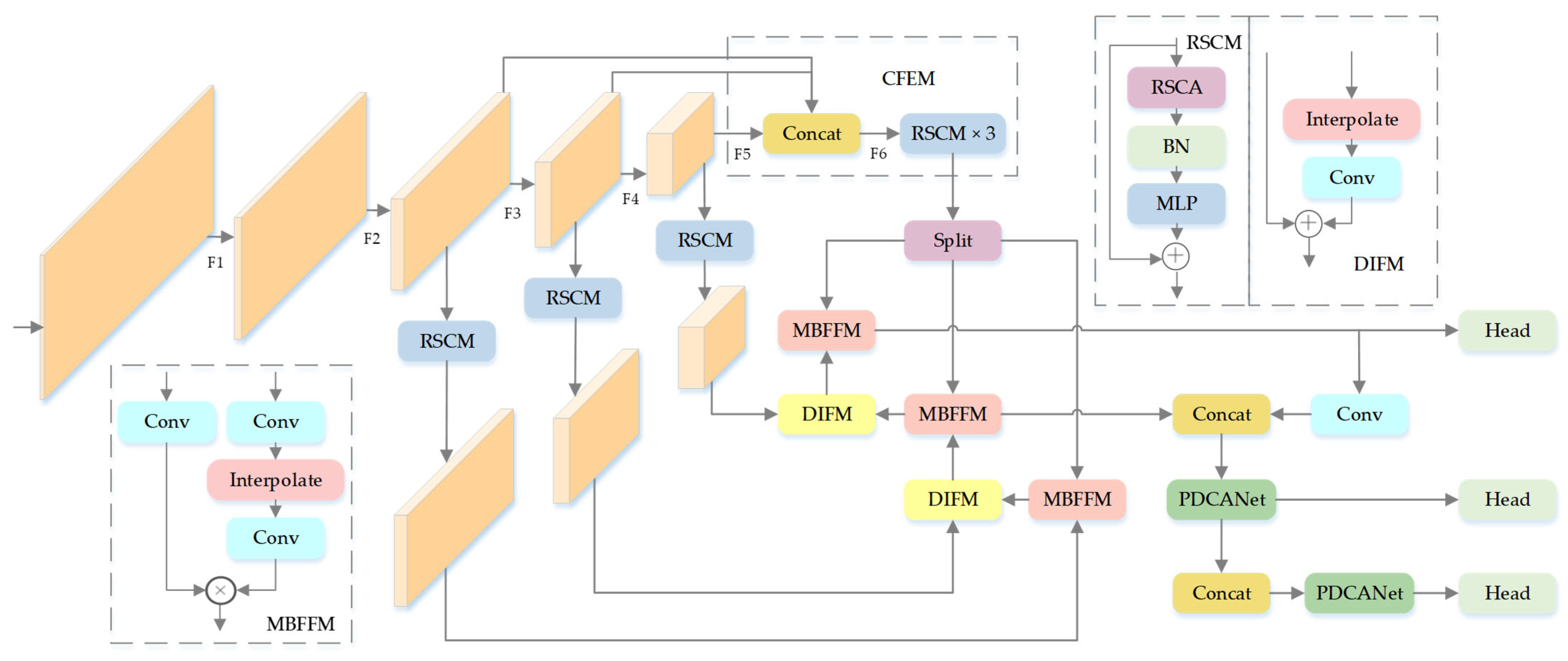
Aiming to merge and synthesize contextual information across multi-scale feature maps to enhance the model’s performance for target detection in complex remote sensing scenarios, we propose MFRFPN for feature pyramid reconstruction. MFRFPN is shown in Figure 4.
A Rectangular Self-Calibration Module (RSCM) is developed to mitigate interference from cluttered backgrounds in remote sensing images and improve foreground feature saliency. In this framework, horizontal and vertical pooling operations are integrated to aggregate multi-scale pyramid features, thereby enabling axial-aware global context modeling. The RSCM consists of three components: Rectangular Self-Calibration Attention (RSCA), BN, and Multi-Layer Perceptron (MLP). RSCA implements hybrid attention by merging multi-scale spatial context modeling and channel-wise feature reweighting, which jointly mitigates semantic conflicts to boost discriminative power. Additionally, the RSCM employs an MLP to further strengthen feature representation.
The RSCA mechanism captures axial global contexts through horizontal and vertical pooling operations, generating two distinct directional feature vectors. These vectors undergo broadcast addition to effectively model ROIs. A shape self-calibration function aligns these regions with foreground objects using large-kernel strip convolutions decoupled along horizontal and vertical axes. Horizontal strip convolution with k × 1 kernel adjusts row-wise features to approximate object boundaries, with BN and ReLU activation applied subsequently. Vertical strip convolution with 1 × k kernel then performs complementary column-wise calibration. This dual-axis architecture adapts flexibly to arbitrary object geometries, formally expressed as follows:
ξ   c y ¯ = δ   ψ k × 1 ( ϕ   ψ 1 × k y ¯ ) y ¯ = H   P ( x ) V   P ( x )
Here, the symbol ψ denotes the large-kernel strip convolution, and k represents the kernel size of the strip convolution. The symbol ϕ corresponds to BN followed by the ReLU activation function. H   P and V   P represent horizontal pooling and vertical pooling, respectively. Notably, the numeral δ is used here to denote the Sigmoid function. The symbol ξ   c denotes the output feature of the RSCA mechanism.
Additionally, a hybrid fusion framework merges augmented attention features and raw inputs, leveraging 3 × 3 depthwise convolutional kernels to preserve structural details while suppressing redundant activations. Refined input features and calibrated attention vectors are combined through Hadamard product, which enhances discriminative feature propagation while preserving computational efficiency.
ξ   F x , y = ψ 3 × 3 ( x ) y
Here, the operator ψ 3 × 3 denotes depth-wise convolution with a 3 × 3 kernel, and y represents the attention features obtained from the preceding step. The symbol indicates the Hadamard product.
BN and MLP are incorporated after RSCA to refine the features. Finally, residual connections are embedded to strengthen gradient flow and feature propagation. The schematic of RSCM depicted in Figure 4 is mathematically expressed as follows:
F   o u t = ρ   ξ   F ( x , ξ   c ( H   P ( x ) V   P ( x ) ) ) + x
Here, denotes broadcast addition. ξ   F represents the feature fusion function that integrates depth-wise convolution and the Hadamard product to enhance discriminative features. The attention feature ξ   c is fused with the original feature through depth-wise separable convolution and element-wise multiplication, enabling dynamic feature weighting. This process strengthens salient features while suppressing irrelevant ones. The symbol ρ denotes a composite operation consisting of BN and an MLP. It is applied to the fused feature for normalization and nonlinear transformation, thereby enhancing the semantic representation capability.
To extract contextual information, enrich semantic features, and enhance model performance, the feature pyramid is redesigned through multi-scale integration, while the Contextual Feature Extraction Module (CFEM) is introduced to enhance cross-level dependency modeling. The backbone generates feature maps with multiple scales   F   1 ,   F   2 ,   F 3 ,   F   4 ,   F   5 at different stages, with resolutions [ H 2 × W 2 , H 4 × W 4 , H 8 × W 8 , H 16 × W 16 , H 32 × W 32 ], which are utilized for subsequent detection and segmentation tasks. To ensure computational efficiency, the large-scale features F1 and F2 are discarded. The lower-scale features F3, F4 and F5 are down-sampled to H 64 × W 64 via average pooling and then combined via concatenation to construct the pyramid feature F6. Subsequently, F6 is fed into a series of stacked RSCM modules for further processing. The RSCM module captures axial global contextual information by integrating multi-scale pyramid features, thereby enhancing the saliency of foreground features. Subsequent to pyramidal feature fusion, the consolidated features are split and reconstructed via adaptive up-sampling, thereby recovering their original scales. This process is formulated as follows:
P = R S C M   A P   ( F 3 , 8 , A P   F   4 , 4 , A P   ( F   5 , 2 ) )
where A P   ( F , x ) denotes average pooling with a down-sampling factor x applied to feature F, and P represents the feature with pyramid context.
The Dynamic Interpolation Fusion Module (DIFM) is engineered to fuse feature maps across multiple scales by dynamically integrating low-resolution features with processed high-resolution features. The module takes two inputs: a low-resolution feature map and a high-resolution feature map. First, the high-resolution feature map is adaptively scaled via bilinear interpolation to align spatial resolutions with the low-resolution counterpart. Spatially up-sampled high-resolution features undergo 1 × 1 convolution-based channel adaptation, ensuring dimensional consistency with low-resolution feature hierarchies. Finally, the processed high-resolution features are element-wise summed with the low-resolution features to generate the fused output.
The MBFFM focuses on local feature refinement through nonlinear transformations and Hadamard products, effectively suppressing background noise while enhancing discriminative patterns. The DIFM emphasizes dynamic scale calibration, integrating multi-scale features using bilinear interpolation and channel-wise adaptation. MBFFM operates at the branch level within the feature pyramid, emphasizing nonlinear interactions between branches to suppress redundant activations and enhance key feature regions. DIFM, on the other hand, addresses the dynamic alignment of cross-scale features during global reconstruction, ensuring complementarity among multi-scale information.
The Multi-Branch Feature Fusion Module (MBFFM) integrates feature maps of different resolutions through convolution operations and activation functions. The module takes two inputs: a low-resolution feature map and a high-resolution feature map. First, the high-resolution feature map undergoes convolution followed by an h-sigmoid activation function for nonlinear transformation. It is then up-sampled via bilinear interpolation to align with the spatial resolution of the low-resolution features. Finally, the processed high-resolution features are element-wise multiplied with the convolved low-resolution features. This mechanism suppresses feature responses in irrelevant regions while enhancing critical semantic representations, enabling dynamic feature selection through hierarchical fusion.
The MFRFPN integrates low-level spatial and high-level semantic features across corresponding scales. The CFEM module is utilized to reconstruct fused features. The RSCM captures axial global context to model bounding boxes of interest, while the shape self-calibration function refines attention maps toward foreground objects. A feature pyramid guides the spatial feature reconstruction, ensuring multi-scale awareness in the reconstructed features.

3.3. Efficient Feature Enhancement Strategy

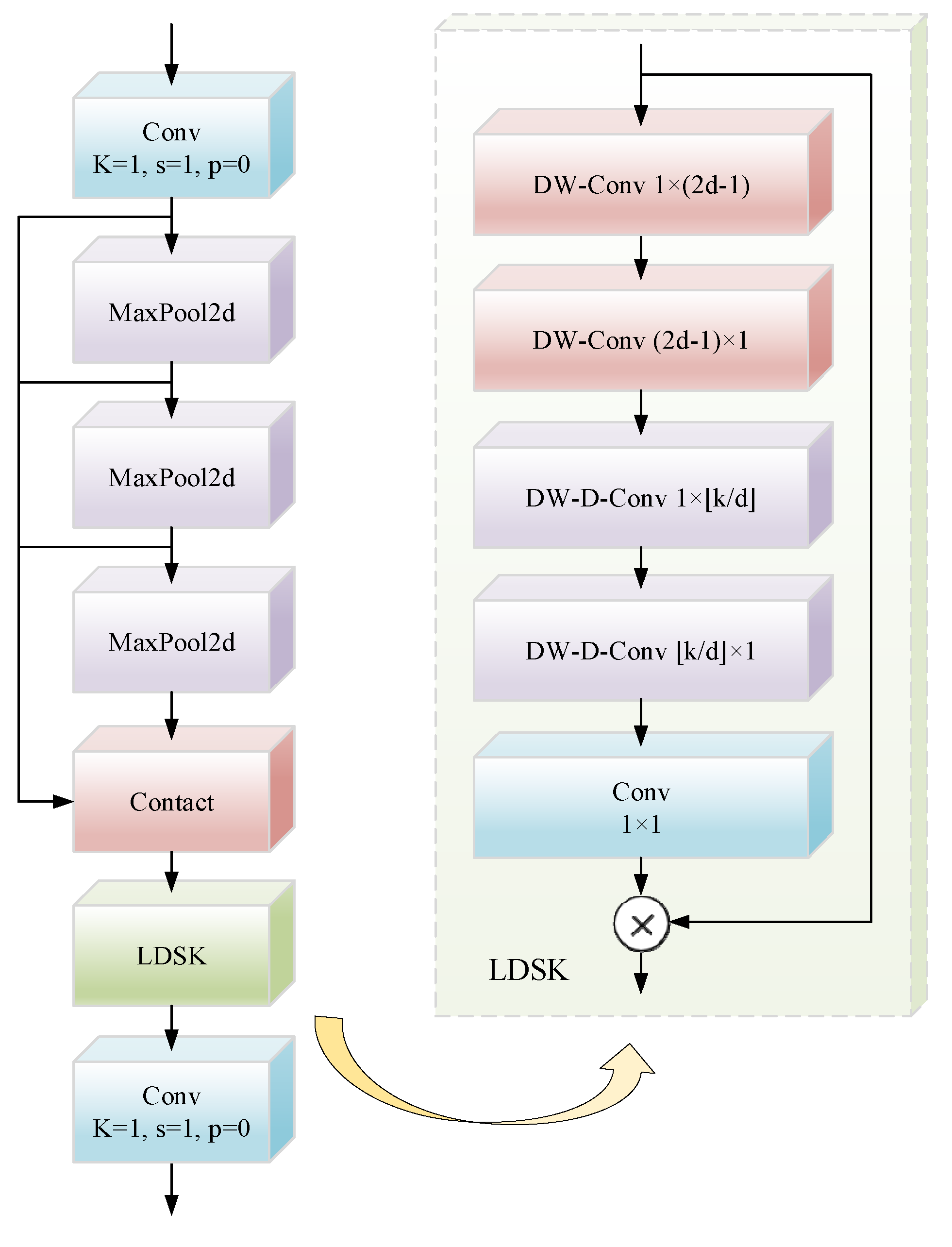
The SPPF module undertakes the tasks of feature extraction and encoding at multiple scales. This enables the integration of multi-scale features, with the aim of enhancing the semantic representations of feature maps. To enhance the architecture’s feature augmentation capability, we proposed LDSK, as depicted in Figure 5. The LDSK significantly improves the SPPF’s ability to aggregate features across scales. By leveraging large depth-separable kernels and dilated spatial convolutions, the LDSK captures broad contextual information from images, generates attention maps, and uses these maps to adaptively weight the original features. This mechanism strengthens the network’s focus on discriminative patterns, thereby improving model performance.
Traditional dilated convolution enhances feature extraction by expanding the receptive field, but it often leads to a significant increase in parameter count. Attention mechanisms typically rely on global pooling and fully connected layers to generate channel-wise or spatial attention weights, introducing additional computational overhead. In contrast, LDSK employs 1D separable convolutions to reduce the number of parameters and avoid the complex weight generation process, thereby significantly improving computational efficiency. Moreover, conventional dilated convolution tends to suffer from sparse sampling under large dilation rates, resulting in the loss of local details. Although attention mechanisms focus on key regions through learned weights, they involve complex computations. The LDSK module addresses these issues by decomposing convolution kernels to achieve implicit axial global context modeling. Its adaptive dilation rate design extends the receptive field while preserving local continuity, making it particularly effective for capturing contextual patterns in remote sensing images with complex structures.
The LDSK’s structure and function are categorized into three essential steps: initialization convolution layer, spatially dilated convolution layer, and attention fusion/application. Initialization Convolution layer: LDSK decomposes 2D convolution kernels into horizontal and vertical 1D kernels. These two convolutional layers separately extract horizontal and vertical directional features from input feature maps, enabling the model to enhance saliency localization. The LDSK module employs dilated convolutions with multi-scale dilation rates in its dedicated layer to refine features extracted from preliminary attention maps. Spatially dilated convolution layer: After obtaining preliminary attention maps, LDSK uses spatially dilated convolutions with varying dilation rates to further extract features. Through cascaded 1D convolution kernels, LDSK simultaneously captures both local and global contextual information. These layers expand receptive fields to aggregate extensive contextual features while processing horizontal and vertical directions independently, enhancing spatial relationship understanding. Attention fusion and application: Following the convolution operations, the LDSK integrates features via the terminal convolutional layer to produce optimized attention maps. These maps undergo element-wise multiplication with the original input features, dynamically weighting significant features while suppressing irrelevant ones. The output is derived as follows:
Z ¯ C = H , W W ( 2 d 1 ) × 1 C ( H , W W 1 × 2 d 1 C F C ) Z C = H , W W k d × 1 C ( H , W W 1 × k d C Z ¯ C ) A C = W 1 × 1 Z C F ¯ C = A C F C
Given an input feature map F R C × H × W , where C denotes the number of input channels, H and W represent the height and width, d is the dilation rate, k indicates the maximum receptive field of the kernel, and ⌊⋅⌋ denotes the floor operation. The symbols ∗ and represent convolution and Hadamard product, respectively. Z ¯ C denotes the output of the depth-wise convolution. Z C represents the output of the dilated depth-wise convolution. A 1 × 1 convolution refines the outputs of the dilated depth-wise convolution, producing the attention map A C . The output F ¯ C is obtained via the Hadamard product between A C and the input feature map F C .
The choice of hyper parameters in the LDSK module is based on the need to balance receptive field expansion and computational efficiency while addressing the unique challenges of remote sensing images. Thus, we selected k = 11 and d = 2. In the LDSK module, the convolutional kernel size is set to K = 11. This is because in feature extraction, the kernel size needs to cover the typical scale of small targets. The large kernel matches small target clusters in remote sensing images and aligns with SPPF output features to avoid disconnection. For computational efficiency, the kernel is decomposed into two 1D kernels, reducing parameters while maintaining spatial modeling ability and receptive field. The dilation rate in the LDSK module is set to d = 2. Remote sensing images often have dense small targets. This rate ensures sufficient context coverage and avoids over-smoothing. It prevents overfitting in cascaded layers and captures multi-scale contexts. This design adapts to the large scale variations of targets in remote sensing images. The rate expands the receptive field without increasing kernel size or causing aliasing artifacts. It also aligns with the feature pyramid levels of MFRFPN. A d = 2 rate balances global context capture and training stability.

3.4. Hybrid Loss

Unlike natural imagery, remote sensing imagery demonstrates a higher density of small-scale objects. However, traditional IoU metrics are inherently prone to positional variations in small objects, which makes it challenging to provide sufficient high-quality samples for object detectors and degrades detection performance. A hybrid loss training strategy is introduced to optimize small-scale target discriminability.
To enhance object detection performance, NWD is adopted to quantify the distribution between bounding boxes. This metric is then converted into a similarity measure and trained alongside the original IoU. NWD smooths positional deviations and better characterizes the weight distribution of different pixels within bounding boxes. More importantly, it remains scale-insensitive and is better suited for assessing similarity among tiny objects. By modeling bounding box A = ( c x a ,   c y a ,   w a ,   h a ) and bounding box B = ( c x b ,   c y b ,   w b ,   h b ) as 2D Gaussian distributions, we derive the squared Wasserstein distance w 2 2 ( N a , N b ) . Nevertheless, since w 2 2 ( N a , N b ) is unsuitable for direct use as a similarity measure, an exponential normalization is applied to obtain NWD:
N W D ( N a , N b ) = e x p ( w 2 2 ( N a , N b ) c )
where c is a dataset-specific constant. The bounding box loss functions are formulated as follows:
L N W D = 1 N W D N a , N b L o b j = 1 I O U r a t i o × L N W D + I O U r a t i o × L i o u
Here, I O U r a t i o serves as a modulation coefficient.
The hybrid loss function integrates NWD and IoU metrics via a dynamic weighting mechanism, with each loss component’s contribution modulated by a predefined IoU ratio parameter. Based on ablation experiments on the NWPU-VHR10 and VEDAI datasets, setting this ratio at 0.5 achieves the best balance between localization accuracy and robustness to positional deviations. This setting balances IoU’s sensitivity to boundary alignment with NWD’s scale-invariant similarity measurement. Lower values reduce background noise suppression, while higher values degrade performance due to overemphasis on strict IoU alignment—particularly problematic for small objects with sparse pixel coverage. NWD’s robustness to scale changes reduces the scale sensitivity of IoU, making it ideal for detecting small objects with amplified positional deviations. A 50% weight ensures NWD dominates gradient updates for small targets, while IoU’s localization sensitivity provides strong gradients for precise boundary alignment, complementing NWD’s global similarity measurement. This 50% weighting also ensures adequate localization refinement for larger objects or cases with clear spatial boundaries.

4. Experiment and Result

4.1. Experimental Datasets

The NWPU-VHR10 dataset [38] comprises 800 images. It is divided into two subsets: a positive image set containing 650 images with at least one target object, and a negative image set with 150 background-only images. The annotated objects span 10 categories: airplane, ship, storage tank, baseball diamond, tennis court, basketball court, athletics field, harbor, bridge, and vehicle. The dataset is divided into training, testing, and validation sets following a 7:2:1 allocation ratio.
The VEDAI dataset [39] is a multispectral aerial vehicle detection dataset containing both visible-spectrum and infrared image modalities. Its images cover diverse environments and weather conditions, enhancing model generalizability. The dataset includes 1246 images with annotations for 8 object categories: car, truck, pickup truck, tractor, camper van, boat, motorcycle, and bus. Data splits follow a 7:2:1 ratio for training, testing, and validation sets.

4.2. Experimental Details and Evaluation Indicators

The experimental configuration of the present study is summarized below. All experiments were executed on an Ubuntu 22.04-equipped server, with Python 3.12.3 employed for model training and CUDA 12.1 leveraged for GPU acceleration. Implementations were developed within the PyTorch framework. Training was performed on the NVIDIA RTX 4090 GPU with 24 GB memory. The SGD optimizer was utilized with an initial learning rate of 0.01 to facilitate parameter adjustments in advanced training phases and enhance model generalization capabilities. Input images underwent size adjustment to 640 × 640 pixels, with mosaic data augmentation applied during preprocessing. A warmup strategy with a momentum of 0.8 was utilized during the first three epochs to stabilize early training phases. Early stopping was implemented based on validation metric optimization. For both the NWPU-VHR10 and VEDAI datasets, the model underwent 300-epoch training with a batch size configuration of 16. Other detection models were evaluated using the default configurations specified in their respective original publications. Key training parameters are detailed in Table 1.
Model evaluation employs four key metrics: Precision (P), Recall (R), and mAP. Precision evaluates the ratio of correctly identified positive predictions among all predicted positive instances, whereas Recall measures the ratio of correctly identified objects relative to all ground-truth positives. These metrics are derived from true positives (TPs), false positives (FPs), true negatives (TNs), and false negatives (FNs). The formula for calculating the evaluation metrics is as follows:
P = T P T P + F P R = T P T P + F N
Average Precision (AP) is computed as the area under the P-R curve. The mAP is calculated by aggregating per-class AP values through mean computation, serving as a holistic evaluation metric. We usually use mAP values to evaluate the accuracy of the model. The definitions of AP and mAP are formalized as follows:
A P = 0 1 P ( R ) d R m A P = 1 N i = 1 N A P ( i )

4.3. Ablation Experiments

To verify the MCRS-YOLO network’s enhancement efficacy, we conducted ablation studies on the NWPU-VHR10 and VEDAI datasets using the YOLOv11n baseline. The experiments incrementally integrated proposed enhancements to evaluate their individual contributions, with eight sub-experiments per dataset. All models were trained under identical hyper parameters for fair comparison. Table 2 and Table 3 display the experimental results, where the “√” symbol denotes the inclusion of each module in the corresponding configuration. Performance metrics P, R, mAP, parameter count, and GFLOPS demonstrate the efficacy of our methods. The ablation study design is as follows:
A: develop the MBA to enrich object information for small targets.
B: design the MFRFPN structure in the neck network to reconstruct the feature pyramid and fuse multi-scale features.
C: propose the LDSK to expand the receptive field and enhance feature extraction.
D: implement the NWD hybrid loss training strategy to suppress background noise.
Table 2. Ablation study on the NWPU VHR-10 dataset.
ModelABCDPRmAPParamFLops
Baseline 0.8740.870.9172.6 M6.3 G
0.8760.8810.9243.2 M7.3 G
0.9070.8730.9313.3 M8.6 G
0.9060.8560.9232.8 M6.5 G
0.8990.8810.9272.5 M6.3 G
0.9140.8960.9383.9 M9.4 G
0.9230.8980.9474.1 M9.6 G
ours0.9470.8980.9574.1 M9.6 G
Table 3. Ablation study on the VEDAI dataset.
ModelABCDPRmAPParamFLops
Baseline 0.6230.5740.5792.6 M6.3 G
0.70.5650.5893.2 M7.3 G
0.7050.5780.6053.3 M8.6 G
0.6770.5720.5932.8 M6.5 G
0.6980.5690.5962.5 M6.3 G
0.7160.5750.6163.9 M9.4 G
0.7380.5760.6324.1 M9.6 G
ours0.7420.580.6464.1 M9.6 G
Table 2 and Table 3 validate that MCRS-YOLO achieves significantly improved detection performance. The MFRFPN reconstructs the feature pyramid by extracting features from global contextual information and performing multi-scale feature fusion. Despite its architectural complexity introducing an additional computational burden, the enhancements to the network aim to enhance channel–spatial information, expand the effective receptive field, and suppress background noise, collectively reduce both false positive and false negative rates. These optimizations enhance the overall detection accuracy.
The ablation study results in Table 2 evidence performance gains on the NWPU-VHR10 dataset, with Precision elevated from 0.874 to 0.947, Recall enhanced from 0.87 to 0.898, and mAP boosted from 0.917 to 0.957, confirming substantial model optimization efficacy. The MCRS-YOLO achieves a detection accuracy of 95.7%, significantly outperforming networks with single or combined improvement strategies. The MCRS-YOLO demonstrates a 4% mAP enhancement versus the YOLOv11 baseline. Across all performance metrics, our proposed enhancements surpass the baseline, demonstrating that the refined model efficiently elevates the capabilities of the object detection framework.
The ablation study results in Table 3 evidence performance gains on the VEDAI dataset, with Precision elevated from 0.623 to 0.742, Recall enhanced from 0.574 to 0.58, and mAP boosted from 0.579 to 0.646, underscoring remarkable performance gains. The MCRS-YOLO achieves a detection accuracy of 64.6%, notably surpassing networks employing single or combined improvement strategies. Compared to YOLOv11, the mAP is enhanced by 6.7%. Across all performance metrics, our enhanced solution outperforms the baseline, validating its efficacy in enhancing object detection model performance.
Furthermore, Figure 6 and Figure 7 visualize the feature heatmaps extracted from the YOLOv11 and MCRS-YOLO networks. As shown in rows (a) and (b), the heatmaps in row (a) are extracted from YOLOv11, while those in row (b) are generated by MCRS-YOLO. The color bars (0–1) represent confidence scores, where higher values indicate greater model certainty in detecting targets within corresponding regions.
A comparative analysis of these heatmaps reveals that the improved MCRS-YOLO exhibits significant advantages. In the enhanced model, red high-confidence regions are more concentrated, and blue low-confidence backgrounds are substantially reduced, demonstrating improved localization accuracy and background suppression capability. The heatmaps demonstrate that MCRS-YOLO extracts more discriminative features from images, enhancing the richness and granularity of feature representations while fully leveraging information from densely arranged small objects. These visualizations confirm that MCRS-YOLO strengthens multi-scale feature fusion, resulting in enhanced confidence intensity in target core areas and fewer false positives in background regions. This evidence robustly validates the superior detection performance of MCRS-YOLO in complex remote sensing scenarios. These results indicate that MCRS-YOLO outperforms YOLOv11 in detecting objects in remote sensing imagery.
Meanwhile, the MCRS-YOLO demonstrates significant advantages in reducing both false positives and false negatives, as revealed in the heatmap analysis shown in Figure 6 and Figure 7. The heatmaps indicate that MCRS-YOLO’s high-confidence areas are more focused and accurately cover target objects, with reduced background interference. The blue low-confidence background regions are significantly decreased, reflecting the model’s enhanced ability to suppress complex backgrounds and reduce false positives. The confidence scores for small targets are improved, leading to a lower miss-detection rate and reduced false negatives, particularly in dense target scenarios. This visualization effectively demonstrates the advantages of our method.

4.4. Comparison Experiments

To thoroughly assess MCRS-YOLO’s performance, extensive experiments were executed on the NWPU-VHR10 and VEDAI datasets. These results confirm the excellent performance of MCRS-YOLO in remote sensing object detection tasks. The best performance metrics are highlighted in red, while the second-best results are marked in blue.

4.4.1. Comparative Experiment on Convolutional Networks

We introduced various convolutional networks into the C3k2 module of the baseline YOLOv11 model and conducted comparative experiments on the NWPU VHR-10 and VEDAI datasets. The last row corresponds to our proposed MBA. The results are displayed in Table 4 and Table 5.
As shown in the tables above, the experimental results clearly demonstrate that strategically integrating the MBA module into the YOLOv11 architecture achieves notably superior detection precision with the best mAP value. This remarkable performance improvement stems from MBA’s enhanced gradient flow through strategically synergistic integration of multiple convolutional operations, which strengthens multi-level feature representation and semantic depth, demonstrating highly efficient remote sensing image detection capabilities.

4.4.2. Comparative Experiments on Feature Pyramid Networks

To systematically evaluate architectural improvements, different kinds of feature pyramid network architectures were integrated into the YOLOv11, with comprehensive comparative tests conducted on the NWPU VHR-10 and VEDAI datasets. The results are presented in Table 6 and Table 7.
As demonstrated in the table above, the integration of the proposed MFRFPN architecture into the YOLOv11 framework achieves optimal detection performance. MFRFPN improves multi-scale feature representation, enhancing target recognition in complex backgrounds. Its RSCM captures the axial global context, CFEM strengthens cross-level dependency modeling, and DIFM and MBFFM achieve effective multi-scale feature fusion from different perspectives. This performance improvement stems primarily from the proposed MFRFPN architecture, which enhances multi-scale feature fusion capabilities and optimizes contextual information capturing. The architecture demonstrates exceptional performance in effectively tackling significant variations in object scales and intricate spatial dependencies among remote sensing targets, thereby significantly elevating object detection accuracy in remote sensing imagery.

4.4.3. Comparative Experiments on Spatial Pyramid Pooling Fast

Various feature extraction methods were incorporated into YOLOv11 for comprehensive comparative experiments on the NWPU VHR-10 and VEDAI datasets, with the results summarized in Table 8 and Table 9.
When the proposed LDSK module was integrated into the YOLOv11 framework, it achieved the highest mAP among all evaluated configurations. This superior performance originates from the LDSK module to capture discriminative object features and expand the effective receptive field, demonstrating robust feature extraction capabilities in remote sensing images.

4.4.4. Comparative Experiments on Different IoU Ratios

To further investigate the impact of varying IoU ratios on the NWD, comparative experiments were performed on the YOLOv11 framework using different IoU ratio parameters within the NWD, with the results detailed in Table 10 and Table 11.
The experimental data indicate that an IoU ratio of 0.5 achieves the highest mAP. This optimal performance arises because lower IoU ratio thresholds may fail to enforce precise boundary alignment, allowing detection boxes to overlap with background regions and introduce background noise or partial target inclusions, thereby degrading the model’s spatial localization learning. Conversely, excessively high IoU ratio thresholds require near-perfect overlap between predicted and ground-truth boxes, which causes excessive false negatives for small objects due to strict alignment criteria. Consequently, an IoU ratio of 0.5 is selected for the NWD configuration in our framework.

4.4.5. Comparative Experiments on Different Models

We conducted comparative experiments between various models and the proposed MCRS-YOLO framework. The evaluation framework included single-stage detectors such as YOLO series, as well as two-stage detectors like Faster R-CNN. A comparative analysis was conducted against state-of-the-art detectors. In the final row of the tables, MCRS-YOLO represents our proposed model. To ensure fair comparisons, consistent parameter configurations were maintained across all networks during training. This methodology facilitates an objective assessment of the advantages and effectiveness of MCRS-YOLO in remote sensing imagery detection tasks. The experimental results are presented in Table 12 and Table 13.
As shown in the tables above, MCRS-YOLO outperforms other comparative algorithms in the evaluation metric mAP50. In small-object and dense-scenario detection, the Mask R-CNN algorithm often fails to retain target information. Furthermore, in low-resolution images, both Mask R-CNN and RT-DETR may miss certain targets, leading to false positives or false negatives in complex remote sensing scenarios. Our algorithm was also compared with recently proposed models, including RT-DETR. The MCRS-YOLO achieves higher target detection accuracy in remote sensing imagery with complex backgrounds. Although the Transformer architecture in RT-DETR is capable of capturing global contextual relationships, it lacks sufficient focus on local directional-sensitive regions, which are critical in remote sensing images. As a result, it struggles with precise localization of small objects. Although YOLOv10 adopts an FPN+PAN structure, the cross-scale interaction of low-level features remains limited. In remote sensing images, small objects are predominantly present in low-resolution feature maps. However, YOLOv10 applies attention mechanisms only on high-level features, leaving detailed information from lower layers underutilized. Notably, our algorithm achieves higher recognition accuracy.
The results are shown in Figure 8. The Precision–Recall (P-R) curves in the figure demonstrate the optimal detection performance for distinct object categories on both the NWPU VHR-10 and VEDAI datasets.
In summary, the MCRS-YOLO exhibits robust detection capabilities on both datasets. The architectural refinements in MCRS-YOLO significantly boost its small target detection capability.
To further assess MCRS-YOLO’s efficacy, image samples were randomly selected from the NWPU-VHR10 and VEDAI datasets. Detection experiments were conducted using a number of representative models, and the results are shown in Figure 9 and Figure 10. Rows (a), (b), (c) and (d) compare the detection performance of Mask R-CNN, YOLOv11, RT-DETR and the proposed MCRS-YOLO, respectively. In the figures, green boxes denote TP, blue boxes represent FP, and red boxes indicate FN.
In row (a), the density of the FP and FN bounding boxes is relatively high, showing a large accuracy detection defect, and there are more false positives and missed detections. In row (b), a relatively higher density of FP and FN bounding boxes is observed, indicating prevalent misdetections and missed detections due to insufficient recognition precision. In row (c), although the density of FP and FN bounding boxes is reduced, it is still relatively high, which indicates that the accuracy of target detection is insufficient, and there are still misdetections and missed detections in a relatively large area. In contrast, row (d) exhibits a significant reduction in FP or FN instances, with TP boxes concentrated more accurately around the target regions. A comparative analysis of detection results demonstrates that MCRS-YOLO effectively identifies more targets, significantly reduces both FP and FN rates, and achieves higher localization precision, exhibiting exceptional detection performance. The visual comparisons robustly validate the superior performance in object detection within remote sensing imagery.

5. Conclusions

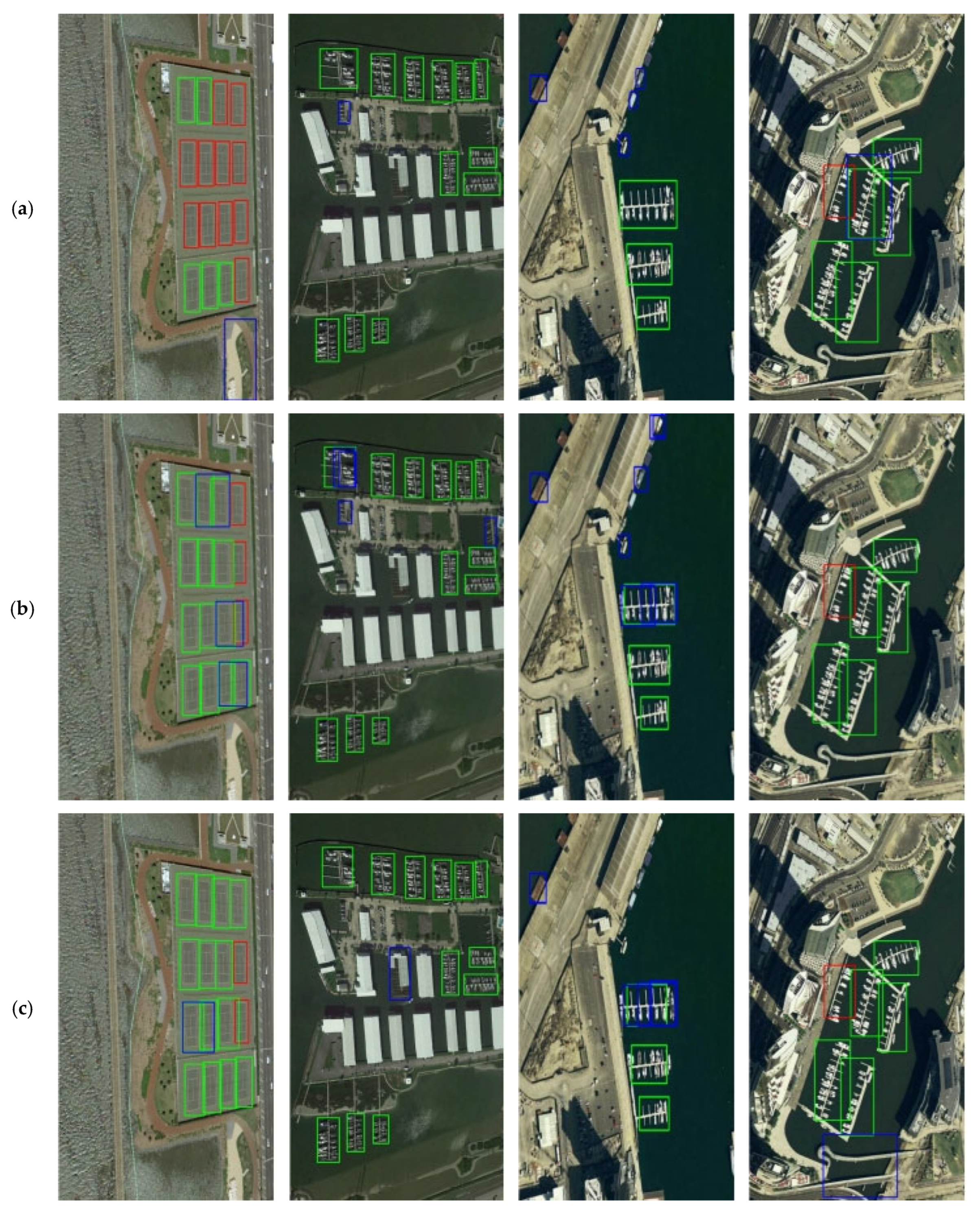
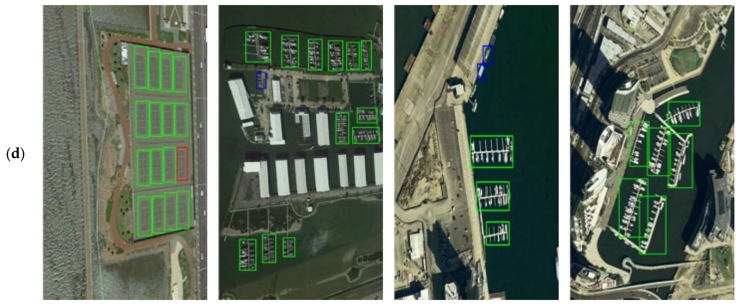
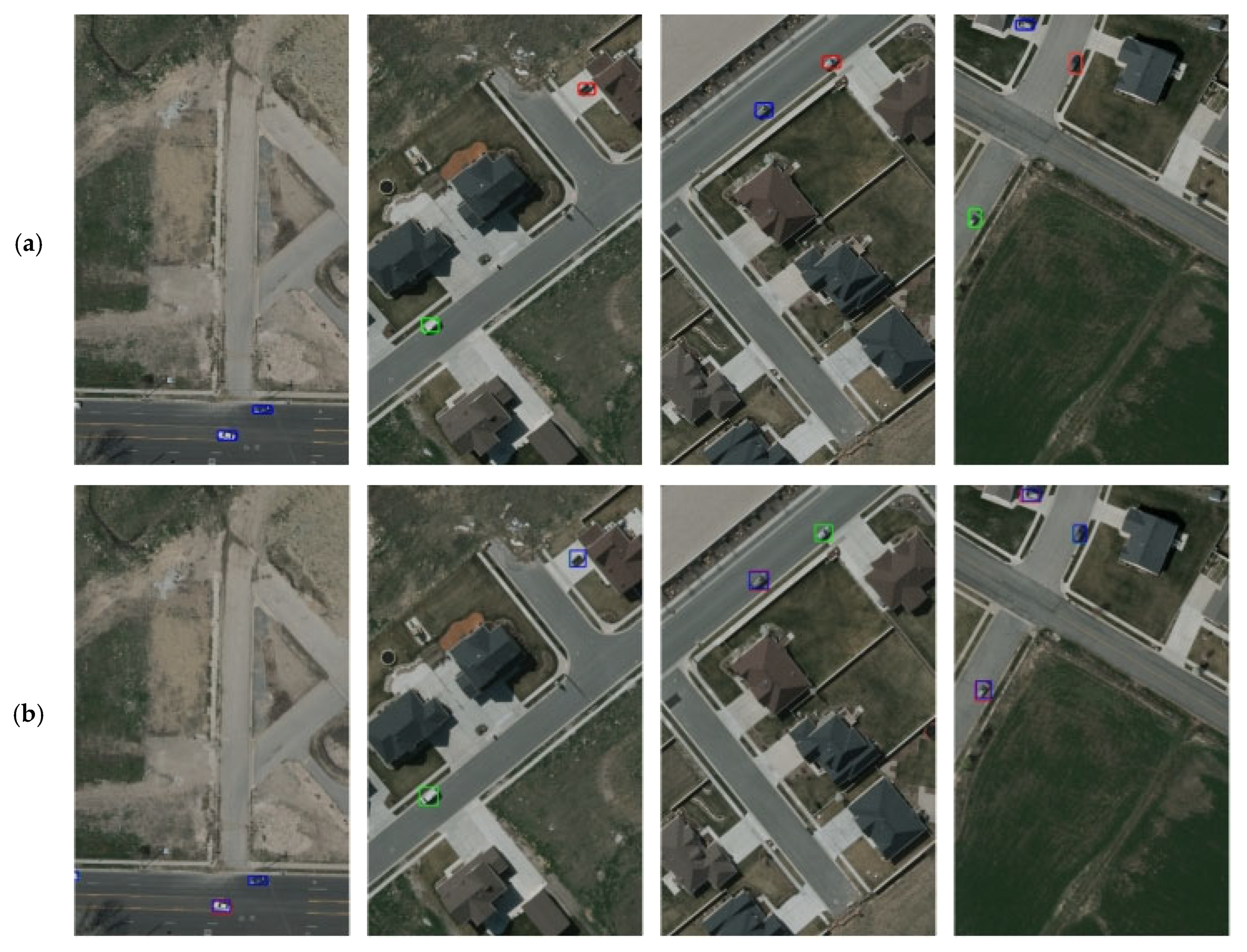
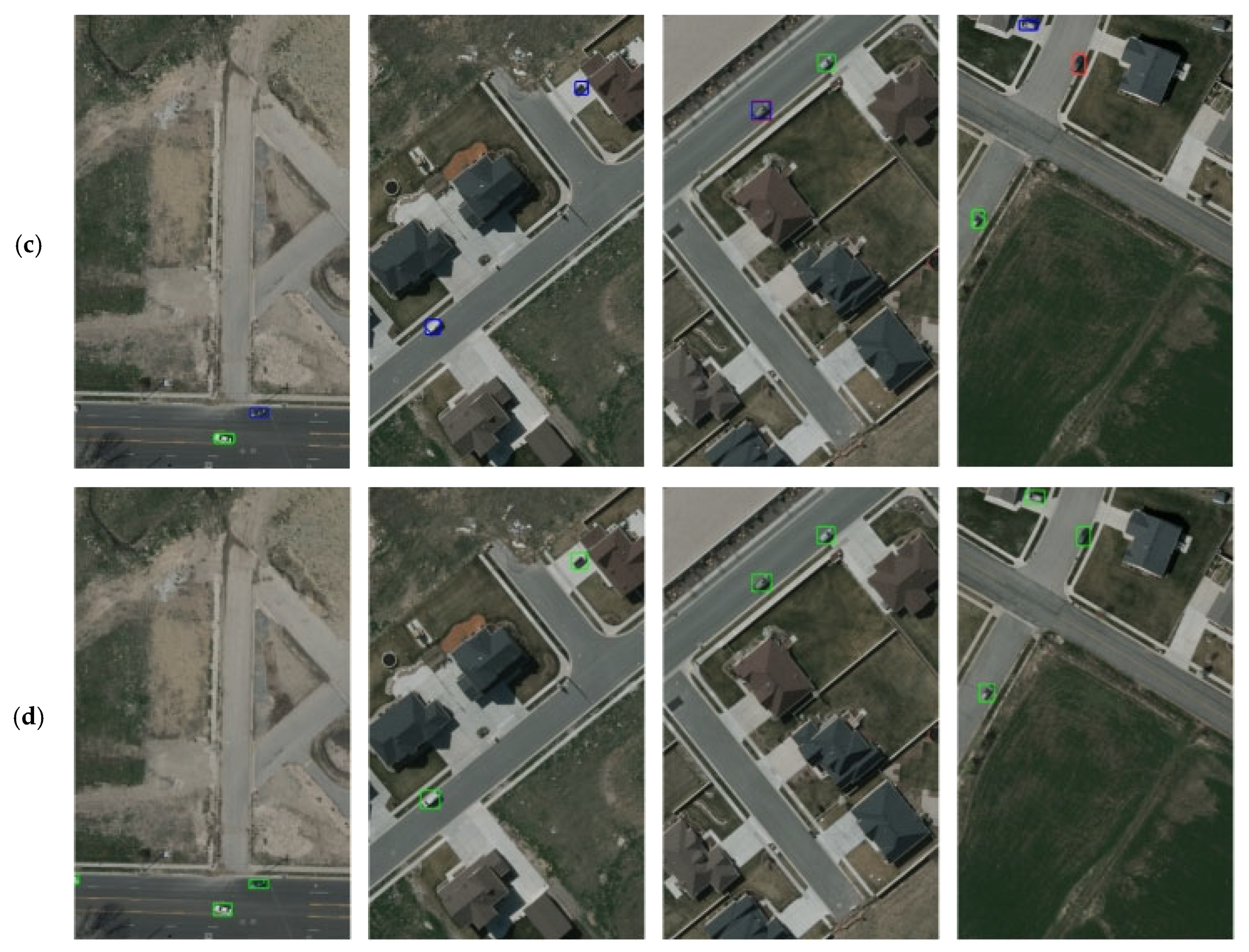
In this paper, a novel small object detection method for remote sensing imagery is proposed, which is termed MCRS-YOLO. Detecting small objects in such images is particularly challenging due to limited object details and complex backgrounds. Conventional operations like pooling, sampling convolutions, and multi-scale feature fusion often lead to a significant loss of spatial information, severely degrading detection accuracy. To mitigate these limitations, we introduce MCRS-YOLO, a model incorporating three key modules: MBA, MFRFPN, and LDSK. Each module uniquely contributes to improving detection performance. MBA enhances feature diversity and information flow through synergistic multi-convolution operations, mitigating insufficient object information. MFRFPN integrates spatially rich multi-scale features to preserve spatial and semantic details. LDSK captures broad contextual information via large-kernel convolutions, expanding the effective receptive field to prioritize critical features. A hybrid loss training strategy combines NWD with IoU loss, reducing sensitivity to positional deviations in small objects while suppressing background noise.
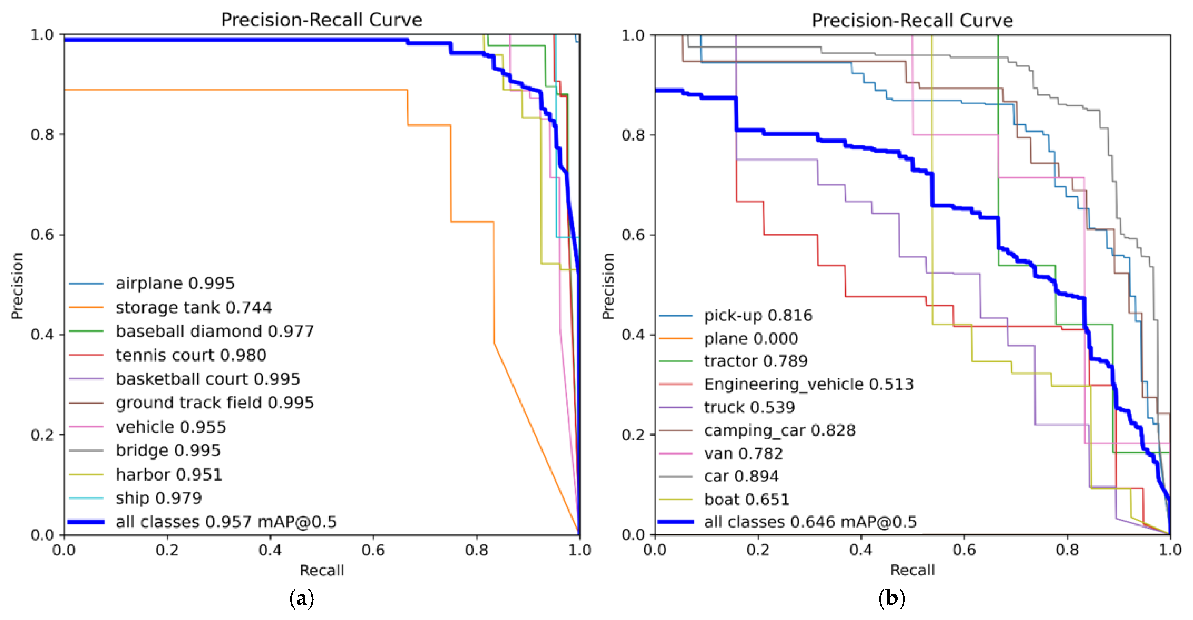
Evaluations on the NWPU-VHR10 and VEDAI datasets reveal that MCRS-YOLO effectively avoids false positives and missed detections when handling significant variations in object scales, dense small targets and cluttered scenes, thereby elevating the accuracy of remote sensing image object detection. Compared to other mainstream models, MCRS-YOLO exhibits superior performance while providing a more efficient and accurate methodology. Future studies will prioritize resolving persisting limitations to strengthen MCRS-YOLO’s adaptability and reliability, targeting algorithm refinements for small object detection in remote sensing imagery and enabling reliable detection capabilities across broader applications and scenarios.

Author Contributions

Conceptualization, L.L.; data curation, L.L. and J.L.; investigation, L.L. and J.L.; methodology, L.L.; software, L.L.; validation, L.L. and J.L.; writing—original draft, L.L.; writing—review and editing, L.L. and J.L.; visualization, L.L.; funding acquisition, J.L. All authors have read and agreed to the published version of the manuscript.

Funding

This research received no external funding.

Data Availability Statement

The original contributions presented in this study are included in this article; further inquiries can be directed to the corresponding author.

Conflicts of Interest

The authors declare no conflicts of interest.

References

  1. Mei, S.; Li, X.; Liu, X.; Cai, H.; Du, Q. Hyperspectral image classification using attention-based bidirectional long short-term memory network. IEEE Trans. Geosci. Remote Sens. 2021, 60, 5509612. [Google Scholar] [CrossRef]
  2. Cheng, G.; Yuan, X.; Yao, X.; Yan, K.; Zeng, Q.; Xie, X.; Han, J. Towards large-scale small object detection: Survey and benchmarks. IEEE Trans. Pattern Anal. Mach. Intell. 2023, 45, 13467–13488. [Google Scholar] [CrossRef] [PubMed]
  3. Shen, C.; Qian, J.; Wang, C.; Yan, D.; Zhong, C. Dynamic sensing and correlation loss detector for small object detection in remote sensing images. IEEE Trans. Geosci. Remote. Sens. 2024, 62, 5627212. [Google Scholar] [CrossRef]
  4. Graziano, M.D. Preliminary Results of Ship Detection Technique by Wake Pattern Recognition in SAR Images. Remote Sens. 2020, 12, 2869. [Google Scholar] [CrossRef]
  5. Liu, X.; He, J.; Yao, Y.; Zhang, J.; Liang, H.; Wang, H.; Hong, Y. Classifying urban land use by integrating remote sensing and social media data. Int. J. Geogr. Inf. Sci. 2017, 31, 1675–1696. [Google Scholar] [CrossRef]
  6. Li, K.; Wang, D.; An, D. Impact of SAR Image Quantization Method on Target Recognition With Neural Networks. IEEE J. Sel. Topics Appl. Earth Observ. Remote Sens. 2025, 18, 308–320. [Google Scholar] [CrossRef]
  7. Bochkovskiy, A.; Wang, C.Y.; Liao, H.Y.M. YOLOv4: Optimal Speed and Accuracy of Object Detection. arXiv 2020, arXiv:2004.10934. [Google Scholar]
  8. Han, J.; Ding, J.; Li, J.; Xia, G.S. Align Deep Features for Oriented Object Detection. IEEE Trans. Geosci. Remote Sens. 2022, 60, 5602511. [Google Scholar] [CrossRef]
  9. Chen, Q.; Xie, Y.; Guo, S.; Bai, J.; Shu, Q. Sensing system of environmental perception technologies for driverless vehicle: A review of state of the art and challenges. Sens. Actuators A 2021, 319, 112566. [Google Scholar] [CrossRef]
  10. Liu, W.; Anguelov, D.; Erhan, D.; Szegedy, C.; Reed, S.; Fu, C.Y.; Berg, A.C. Ssd: Single shot multibox detector. In Proceedings of the Computer Vision–ECCV 2016: 14th European Conference, Amsterdam, The Netherlands, 8–16 October 2016; pp. 21–37. [Google Scholar]
  11. Redmon, J.; Divvala, S.; Girshick, R.; Farhadi, A. You only look once: Unified, real-time object detection. In Proceedings of the 2016 IEEE Conference on Computer Vision and Pattern Recognition (CVPR), Las Vegas, NV, USA, 27–30 June 2016; pp. 779–788. [Google Scholar]
  12. Duan, K.; Bai, S.; Xie, L.; Qi, H.; Huang, Q.; Tian, Q. Centernet: Keypoint triplets for object detection. In Proceedings of the 2019 IEEE/CVF International Conference on Computer Vision (ICCV), Seoul, Republic of Korea, 27 October–2 November 2019; pp. 6568–6577. [Google Scholar]
  13. Girshick, R.; Donahue, J.; Darrell, T.; Malik, J. Rich feature hierarchies for accurate object detection and semantic segmentation. In Proceedings of the 2014 IEEE Conference on Computer Vision and Pattern Recognition, Columbus, OH, USA, 23–28 June 2014; pp. 580–587. [Google Scholar]
  14. Girshick, R. Fast R-CNN. In Proceedings of the 2015 IEEE International Conference on Computer Vision (ICCV), Santiago, Chile, 7–13 December 2015; pp. 1440–1448. [Google Scholar]
  15. Ren, S.; He, K.; Girshick, R.; Sun, J. Faster R-CNN: Towards real-time object detection with region proposal networks. IEEE Trans. Pattern Anal. Mach. Intell. 2016, 39, 1137–1149. [Google Scholar] [CrossRef]
  16. He, K.; Gkioxari, G.; Dollár, P.; Girshick, R. Mask R-CNN. In Proceedings of the 2017 IEEE International Conference on Computer Vision (ICCV), Venice, Italy, 22–29 October 2017; pp. 2980–2988. [Google Scholar]
  17. Khanam, R.; Hussain, M. YOLOv11: An Overview of the Key Architectural Enhancements. arXiv 2024, arXiv:2410.17725. [Google Scholar]
  18. Wang, J.; Xu, C.; Yang, W.; Yu, L. A normalized Gaussian Wasserstein distance for tiny object detection. arXiv 2021, arXiv:2110.13389. [Google Scholar]
  19. Wang, Y.; Wang, B.R.; Huo, L.L.; Fan, Y.S. GT-YOLO: Nearshore Infrared Ship Detection Based on Infrared Images. J. Mar. Sci. Eng. 2024, 12, 213. [Google Scholar] [CrossRef]
  20. Li, Y.; Fan, Q.; Huang, H.; Han, Z.; Gu, Q. A modified YOLOv8 detection network for UAV aerial image recognition. Drones 2023, 7, 304. [Google Scholar] [CrossRef]
  21. Zhang, Y.; Ye, M.; Zhu, G.; Liu, Y.; Guo, P.; Yan, J. FFCA-YOLO for Small Object Detection in Remote Sensing Images. IEEE Trans. Geosci. Remote Sens. 2024, 62, 5611215. [Google Scholar] [CrossRef]
  22. Li, L.; Jiang, L.; Zhang, J.; Wang, S.; Chen, F. A Complete YOLO-Based Ship Detection Method for Thermal Infrared Remote Sensing Images under Complex Backgrounds. Remote Sens. 2022, 14, 1534. [Google Scholar] [CrossRef]
  23. Ma, W.; Li, N.; Zhu, H.; Jiao, L.; Tang, X.; Guo, Y.; Hou, B. Feature split–merge–enhancement network for remote sensing object detection. IEEE Trans. Geosci. Remote Sens. 2022, 60, 5616217. [Google Scholar] [CrossRef]
  24. Fan, X.; Hu, Z.; Zhao, Y.; Chen, J.; Wei, T.; Huang, Z. A small ship object detection method for satellite remote sensing data. IEEE J. Sel. Top. Appl. Earth Obs. Remote Sens. 2024, 17, 11886–11898. [Google Scholar] [CrossRef]
  25. Lin, T.Y.; Dollar, P.; Girshick, R.; He, K.; Hariharan, B.; Belongie, S. Feature pyramid networks for object detection. In Proceedings of the 2017 IEEE Conference on Computer Vision and Pattern Recognition, Honolulu, HI, USA, 21–26 July 2017; pp. 2117–2125. [Google Scholar]
  26. Liu, S.; Qi, L.; Qin, H.; Shi, J.; Jia, J. Path aggregation network for instance segmentation. In Proceedings of the 2018 IEEE Conference on Computer Vision and Pattern Recognition, Salt Lake City, UT, USA, 18–23 June 2018; pp. 8759–8768. [Google Scholar]
  27. Ghiasi, G.; Lin, T.Y.; Le, Q.V. NAS-FPN: Learning scalable feature pyramid architecture for object detection. In Proceedings of the 2019 IEEE/CVF Conference on Computer Vision and Pattern Recognition, Long Beach, CA, USA, 15–20 June 2019; pp. 7036–7045. [Google Scholar]
  28. Tan, M.; Pang, R.; Le, Q.V. EfficientDet: Scalable and efficient object detection. In Proceedings of the 2020 IEEE/CVF Conference on Computer Vision and Pattern Recognition, Seattle, WA, USA, 13–19 June 2020; pp. 10781–10792. [Google Scholar]
  29. Jiang, L.; Yuan, B.; Du, J.; Chen, B.; Xie, H.; Tian, J.; Yuan, Z. MFFSODNet: Multi-Scale Feature Fusion Small Object Detection Network for UAV Aerial Images. IEEE Trans. Instrum. Meas. 2024, 73, 5015214. [Google Scholar] [CrossRef]
  30. Li, X.; Wei, Y.; Li, J.; Duan, W.; Zhang, X.; Huang, Y. Improved YOLOv7 Algorithm for Small Object Detection in Unmanned Aerial Vehicle Image Scenarios. Appl. Sci. 2024, 14, 1664. [Google Scholar] [CrossRef]
  31. Cheng, Y.; Wang, W.; Zhang, W.; Yang, L.; Wang, J.; Ni, H.; Guan, T.; He, J.; Gu, Y.; Tran, N.N. A Multi-Feature Fusion and Attention Network for Multi-Scale Object Detection in Remote Sensing Images. Remote Sens. 2023, 15, 2096. [Google Scholar] [CrossRef]
  32. Jiang, H.; Luo, T.; Peng, H.; Zhang, G. MFCANet: Multiscale Feature Context Aggregation Network for Oriented Object Detection in Remote-Sensing Images. IEEE Access. 2024, 12, 45986–46001. [Google Scholar] [CrossRef]
  33. Tian, P.; Nie, Y. Remote sensing image object detection based on improved YOLOv8. In Proceedings of the Fourth International Conference on Image Processing and Intelligent Control (IPIC 2024), Kuala Lumpur, Malaysia, 23 August 2024; pp. 264–267. [Google Scholar]
  34. Yi, H.; Liu, B.; Zhao, B.; Liu, E. Small object detection algorithm based on improved YOLOv8 for remote sensing. IEEE J. Sel. Top. Appl. Earth Obs. Remote Sens. 2023, 17, 1734–1747. [Google Scholar] [CrossRef]
  35. Zhang, K.; Shen, H. Multi-stage feature enhancement pyramid network for detecting objects in optical remote sensing images. Remote Sens. 2022, 14, 579. [Google Scholar] [CrossRef]
  36. Cheng, G.; Lang, C.; Wu, M.; Xie, X.; Yao, X.; Han, J. Feature enhancement network for object detection in optical remote sensing images. J. Remote Sens. 2021, 2021, 9805389. [Google Scholar] [CrossRef]
  37. Li, W.; Shi, M.; Hong, Z. SCAResNet: A ResNet variant optimized for tiny object detection in transmission and distribution towers. IEEE Geosci. Remote Sens. Lett. 2023, 20, 6011105. [Google Scholar] [CrossRef]
  38. Cheng, G.; Han, J.; Zhou, P.; Guo, L. Multi-class geospatial object detection and geographic image classification based on collection of part detectors. ISPRS J. Photogramm. Remote Sens. 2014, 98, 119–132. [Google Scholar] [CrossRef]
  39. Razakarivony, S.; Jurie, F. Vehicle detection in aerial imagery: A small target detection benchmark. J. Vis. Commun. Image Represent. 2016, 34, 187–203. [Google Scholar] [CrossRef]
  40. Han, k.; Wang, Y.; Guo, J.; Wu, E. ParameterNet: Parameters Are All You Need. arXiv 2023, arXiv:2306.14525. [Google Scholar]
  41. Chen, Z.; He, Z.; Lu, Z.M. Dea-net: Single image dehazing based on detail-enhanced convolution and content-guided attention. IEEE Trans. Image Process. 2024, 33, 1002–1015. [Google Scholar] [CrossRef]
  42. Chen, L.W.; Gu, L.; Zheng, D.Z.; Fu, Y. Frequency-Adaptive Dilated Convolution for Semantic Segmentation. In Proceedings of the 2024 IEEE/CVF Conference on Computer Vision and Pattern Recognition (CVPR), Seattle, WA, USA, 16–22 June 2024; pp. 3414–3425. [Google Scholar]
  43. Cai, X.; Lai, Q.; Wang, Y.; Wang, W.; Sun, Z.; Yao, Y. Poly Kernel Inception Network for Remote Sensing Detection. In Proceedings of the 2024 IEEE/CVF Conference on Computer Vision and Pattern Recognition (CVPR), Seattle, WA, USA, 16–22 June 2024; pp. 27706–27716. [Google Scholar]
  44. Xu, S.; Zheng, S.C.; Xu, W.; Xu, R.; Wang, C.; Zhang, J.; Teng, X.; Li, A.; Guo, L. Hcf-net: Hierarchical context fusion network for infrared small object detection. In Proceedings of the 2024 IEEE International Conference on Multimedia and Expo (ICME), Niagara Falls, ON, Canada, 15–19 July 2024; pp. 1–6. [Google Scholar]
  45. Fan, Q.; Huang, H.; Chen, M.; Liu, H.; He, R. RMT: Retentive Networks Meet Vision Transformers. In Proceedings of the 2024 IEEE/CVF Conference on Computer Vision and Pattern Recognition (CVPR), Seattle, WA, USA, 16–22 June 2024; pp. 5641–5651. [Google Scholar]
  46. Wang, C.; He, W.; Nie, Y.; Guo, J.; Liu, C.; Han, K.; Wang, Y. Gold-yolo: Efficient object detector via gather-and-distribute mechanism. Adv. Neural Inf. Process. Syst. 2023, 36, 51094–51112. [Google Scholar]
  47. Xu, X.; Jiang, Y.; Chen, W.; Huang, Y.; Zhang, Y.; Sun, X. Damo-yolo: A report on real-time object detection design. arXiv 2022, arXiv:2211.15444. [Google Scholar]
  48. Hu, X.; Zhang, P.; Zhang, Q.; Yuan, F. GLSANet: Global-Local Self-Attention Network for Remote Sensing Image Semantic Segmentation. IEEE Geosci. Remote Sens. Lett. 2023, 20, 6000105. [Google Scholar] [CrossRef]
  49. Yang, Z.; Guan, Q.; Zhao, K.; Yang, J.; Xu, X.; Long, H.; Tang, Y. Multi-branch Auxiliary Fusion YOLO with Re-parameterization Heterogeneous Convolutional for Accurate Object Detection. In Proceedings of the Chinese Conference on Pattern Recognition and Computer Vision(PRCV), Urumqi, China, 18–20 October 2024; pp. 492–505. [Google Scholar]
  50. Yang, J.; Li, C.; Dai, X.; Yuan, L.; Gao, J. Focal modulation networks. Adv. Neural Inf. Process. Syst. 2022, 35, 4203–4217. [Google Scholar]
  51. Guo, J.; Chen, X.; Tang, Y.; Wang, Y. Slab: Efficient transformers with simplified linear attention and progressive re-parameterized batch normalization. arXiv 2024, arXiv:2405.11582. [Google Scholar]
  52. Zhao, Y.; Lv, W.; Xu, S.; Wei, J.; Wang, G.; Dang, Q.; Liu, Y.; Chen, J. Detrs beat yolos on real-time object detection. In Proceedings of the 2024 IEEE/CVF Conference on Computer Vision and Pattern Recognition (CVPR), Seattle, WA, USA, 16–22 June 2024; pp. 16965–16974. [Google Scholar]
  53. Lin, T.-Y.; Goyal, P.; Girshick, R.; He, K.; Dollár, P. Focal Loss for Dense Object Detection. In Proceedings of the 2017 IEEE International Conference on Computer Vision (ICCV), Venice, Italy, 22–29 October 2017; pp. 2999–3007. [Google Scholar]
  54. Redmon, J.; Farhadi, A. YOLOv3: An Incremental Improvement. arXiv 2018, arXiv:1804.02767. [Google Scholar]
  55. Ultralytics/yolov5: v7.0—YOLOv5 SOTA Realtime Instance Segmentation. Available online: https://zenodo.org/records/7347926 (accessed on 29 April 2025).
  56. Li, C.; Li, L.; Jiang, H.; Weng, K.; Geng, Y.; Li, L.; Ke, Z.; Li, Q.; Cheng, M.; Nie, W.; et al. YOLOv6: A single-stage object detection framework for industrial applications. arXiv 2022, arXiv:2209.02976. [Google Scholar]
  57. Ultralytics YOLO (Version 8.0.0) [Computer Software]. Available online: https://github.com/ultralytics/ultralytics (accessed on 29 April 2025).
  58. Wang, C.Y.; Yeh, I.H.; Mark Liao, H.Y. Yolov9: Learning what you want to learn using programmable gradient information. In Proceedings of the European conference on computer vision, Milan, Italy, 29 September–4 October 2024; pp. 1–21. [Google Scholar]
  59. Wang, A.; Chen, H.; Liu, L.; Chen, K.; Lin, Z.; Han, J.; Ding, G. Yolov10: Real-time end-to-end object detection. Adv. Neural Inf. Process. Syst. 2024, 37, 107984–108011. [Google Scholar]
  60. Ge, Z.; Liu, S.; Wang, F.; Li, Z.; Sun, J. Yolox: Exceeding yolo series in 2021. arXiv 2021, arXiv:2107.08430. [Google Scholar]
  61. Feng, Y.; Huang, J.; Du, S.; Ying, S.; Yong, J.H.; Li, Y.; Ding, G.; Ji, R.; Gao, Y. Hyper-yolo: When visual object detection meets hypergraph computation. IEEE Trans. Pattern Anal. Mach. Intell. 2024, 47, 2388–2401. [Google Scholar] [CrossRef]
Figure 1. MCRS-YOLO overall architecture.
Remotesensing 17 02204 g001
Figure 2. DSCA architecture overview.
Remotesensing 17 02204 g002
Figure 3. PDCA architecture overview.
Remotesensing 17 02204 g003
Figure 4. MFRFPN architecture overview.
Remotesensing 17 02204 g004
Figure 5. LDSK architecture overview.
Remotesensing 17 02204 g005
Figure 6. Heatmap of NWPU-VHR10 extracted from the network. (a) YOLOv11; (b) MCRS-YOLO.
Remotesensing 17 02204 g006
Figure 7. Heatmap of VEDAI extracted from the network. (a) YOLOv11; (b) MCRS-YOLO.
Remotesensing 17 02204 g007
Figure 8. The detection results of MCRS-YOLO on the different datasets. (a) NWPU VHR-10; (b) VEDAI.
Remotesensing 17 02204 g008
Figure 9. Visualization of TP, FP, and FN on the NWPU-VHR10 dataset. Green boxes represent TP, blue boxes represent FP, and red boxes represent FN. (a) Mask R-CNN; (b) YOLOv11; (c) RT-DETR; (d) MCRS-YOLO.
Remotesensing 17 02204 g009aRemotesensing 17 02204 g009b
Figure 10. Visualization of TP, FP, and FN on the VEDAI dataset. Green boxes represent TP, blue boxes represent FP, and red boxes represent FN (a) Mask R-CNN; (b) YOLOv11; (c) RT-DETR; (d) MCRS-YOLO.
Remotesensing 17 02204 g010aRemotesensing 17 02204 g010b
Table 1. Experiment configuration details.
CategoryParameter
CPU16 vCPU Intel(R) Xeon(R) Gold 6430
GPUNVIDIA RTX 4090 (24 GB)
Python3.12.3
PyTorch2.3.0
CUDA12.1
Training Epochs300
Batch Size16
Weight Decay0.0005
Momentum0.937
Learning Rate0.01
Image Size640
MosaicTrue
Table 4. Comparisons of evaluation indicators on the NWPU VHR-10 dataset.
ModelPRmAPParamFLops
Baseline0.8740.870.9172.6 M6.3 G
+DynamicConv [40]0.8150.8320.8823.5 M6.2 G
+DEConv [41]0.8670.8630.9022.6 M6.3 G
+FADC [42]0.8740.8890.8922.6 M6.3 G
+PKINet [43]0.8430.8790.9132.6 M7.7 G
+HCFNet [44]0.8690.8560.8712.8 M7.1 G
+RetBlock [45]0.8850.8350.8762.5 M6.2 G
OURS0.8760.8810.9243.2 M7.3 G
Red: The best results are marked in red. Blue: The second-best results are marked in blue.
Table 5. Comparisons of evaluation indicators on the VEDAI dataset.
ModelPRmAPParamFLops
Baseline0.6230.5740.5792.6 M6.3 G
+DynamicConv [40]0.580.5450.5513.5 M6.2 G
+DEConv [41]0.660.5620.5782.6 M6.3 G
+FADC [42]0.6140.5340.5812.6 M6.3 G
+PKINet [43]0.5910.5240.5322.6 M7.7 G
+HCFNet [44]0.6230.5640.5672.8 M7.1 G
+RetBlock [45]0.5640.5520.5632.5 M6.2 G
OURS0.70.5650.5893.2 M7.3 G
Red: The best results are marked in red. Blue: The second-best results are marked in blue.
Table 6. Comparisons of evaluation indicators on the NWPU VHR-10 dataset.
ModelPRmAPParamFLops
Baseline0.8740.870.9172.6 M6.3 G
+BiFPN [28]0.8520.8590.9182.0 M6.3 G
+Gold-YOLO [46]0.8940.880.9125.9 M9.2 G
+RepGFPN [47]0.9050.8620.8963.7 M8.2 G
+GLSA [48]0.8960.8670.9263.7 M8.6 G
+MAFPN [49]0.8220.8570.8952.7 M7.1 G
OURS0.9070.8730.9313.3 M8.6 G
Red: The best results are marked in red. Blue: The second-best results are marked in blue.
Table 7. Comparisons of evaluation indicators on the VEDAI dataset.
ModelPRmAPParamFLops
Baseline0.6230.5740.5792.6 M6.3 G
+BiFPN [28]0.6590.5360.5472.0 M6.3 G
+Gold-YOLO [46]0.6640.5410.5515.9 M9.2 G
+RepGFPN [47]0.6730.4460.5183.7 M8.2 G
+GLSA [48]0.6680.5030.5523.7 M8.6 G
+MAFPN [49]0.6170.5710.5412.7 M7.1 G
OURS0.7050.5780.6053.3 M8.6 G
Red: The best results are marked in red. Blue: The second-best results are marked in blue.
Table 8. Comparisons of evaluation indicators on the NWPU VHR-10 dataset.
ModelPRmAPParamFLops
Baseline0.8740.870.9172.6 M6.3 G
+Focal Modulation [50]0.87408490.9192.7 M6.4 G
+RepBN [51]0.8410.7610.8333.2 M6.6 G
+AIFI [52]0.8920.8520.9213.2 M6.6 G
OURS0.9060.8560.9232.8 M6.5 G
Red: The best results are marked in red. Blue: The second-best results are marked in blue.
Table 9. Comparisons of evaluation indicators on the VEDAI dataset.
ModelPRmAPParamFLops
Baseline0.6230.5740.5792.6 M6.3 G
+Focal Modulation [50]0.5960.4940.5892.7 M6.4 G
+RepBN [51]0.5180.4710.4733.2 M6.6 G
+AIFI [52]0.6740.5650.5893.2 M6.6 G
OURS0.6770.5720.5932.8 M6.5 G
Red: The best results are marked in red. Blue: The second-best results are marked in blue.
Table 10. Comparisons of evaluation indicators on the NWPU VHR-10 dataset.
ModelIOU RatioPRmAP
Baseline 0.8740.870.917
+NWD0.40.8650.8710.905
0.450.8790.8820.92
0.50.8990.8810.927
0.550.8940.8670.915
0.60.8870.8620.901
Red: The best results are marked in red. Blue: The second-best results are marked in blue.
Table 11. Comparisons of evaluation indicators on the VEDAI dataset.
ModelIOU RatioPRmAP
Baseline 0.6230.5740.579
+NWD0.40.5960.5710.567
0.450.6390.5620.584
0.50.6980.5690.596
0.550.6790.5540.577
0.60.6620.5420.564
Red: The best results are marked in red. Blue: The second-best results are marked in blue.
Table 12. Comparisons of evaluation indicators on the NWPU VHR-10 dataset.
ModelPRmAPParamFLops
Faster R-CNN [15]0.8820.8450.87460.7 M275.4 G
Mask R-CNN [16]0.8860.8560.87663.4 M329.7 G
RetinaNet [53]0.8750.8420.86935.7 M299.5 G
CenterNet [12]0.8790.8520.88270.6 M137.4 G
YOLOv3 [54]0.880.8130.879103.7 M282.3 G
YOLOv5n [55]0.8490.8960.892.5 M7.1 G
YOLOv5s0.8050.8890.9069.1 M23.8 G
YOLOv6n [56]0.8850.8180.9084.2 M11.8 G
YOLOv6s0.8520.8240.86816.3 M44.0 G
YOLOv8n [57]0.9170.8670.9263.0 M8.1 G
YOLOv8s0.9480.7890.9211.1 M28.5 G
YOLOv9m [58]0.8980.9010.92920.2 M77 G
YOLOv9s0.8380.8530.887.2 M26.7 G
YOLOv10n [59]0.8890.8760.9182.7 M8.2 G
YOLOv10s0.9440.8280.9258.1 M24.5 G
YOLOv11n [17]0.8740.870.9172.6 M6.3 G
YOLOX [60]0.8910.8450.8928.9 M48.1 G
Hyper-yolo [61]0.9210.8940.9314.1 M9.2 G
RT-DETR [52]0.8710.8750.93465.5 M222.5 G
OURS0.9470.8980.9574.1 M9.6 G
Red: The best results are marked in red. Blue: The second-best results are marked in blue.
Table 13. Comparisons of evaluation indicators on the VEDAI dataset.
ModelPRmAPParamFLops
Faster R-CNN [15]0.6910.5710.62560.7 M186.4 G
Mask R-CNN [16]0.7120.5970.63163.4 M240.6 G
RetinaNet [53]0.6790.5510.61435.7 M299.5 G
CenterNet [12]0.6670.5740.58770.6 M137.4 G
YOLOv3 [54]0.7240.4660.567103.7 M282.2 G
YOLOv5n [55]0.60.5940.5492.5 M7.1 G
YOLOv5s0.6630.5260.5659.1 M23.8 G
YOLOv6n [56]0.6210.5640.5824.2 M11.8 G
YOLOv6s0.5870.4870.51316.3 M44.0 G
YOLOv8n [57]0.7190.550.5893.0 M8.1 G
YOLOv8s0.6920.5650.60111.1 M28.5 G
YOLOv9m [58]0.680.5480.55220.1 M76.5 G
YOLOv9s0.6870.5330.5487.2 M26.7 G
YOLOv10n [59]0.6020.6070.5762.7 M8.2 G
YOLOv10s0.7220.4620.5388.1 M24.5 G
YOLOv11n [17]0.6230.5740.5792.6 M6.3 G
YOLOX [60]0.6310.5670.5848.9 M48.1 G
Hyper-yolo [61]0.6140.5790.6124.1 M9.2 G
RT-DETR [52]0.730.4740.61565.5 M222.5 G
OURS0.7420.580.6464.1 M9.6 G
Red: The best results are marked in red. Blue: The second-best results are marked in blue.
Disclaimer/Publisher’s Note: The statements, opinions and data contained in all publications are solely those of the individual author(s) and contributor(s) and not of MDPI and/or the editor(s). MDPI and/or the editor(s) disclaim responsibility for any injury to people or property resulting from any ideas, methods, instructions or products referred to in the content.

