An Optimal Viewpoint-Guided Visual Indexing Method for UAV Autonomous Localization

Abstract

The autonomous positioning of drone-based remote sensing plays an important role in navigation in urban environments. Due to GNSS (Global Navigation Satellite System) signal occlusion, obtaining precise drone locations is still a challenging issue. Inspired by vision-based positioning methods, we proposed an autonomous positioning method based on multi-view reference images rendered from the scene’s 3D geometric mesh and apply a bag-of-words (BoW) image retrieval pipeline to achieve efficient and scalable positioning, without utilizing deep learning-based retrieval or 3D point cloud registration. To minimize the number of reference images, scene coverage quantification and optimization are employed to generate the optimal viewpoints. The proposed method jointly exploits a visual-bag-of-words tree to accelerate reference image retrieval and improve retrieval accuracy, and the Perspective-n-Point (PnP) algorithm is utilized to obtain the drone’s pose. Experiments are conducted in urban real-word scenarios and the results show that positioning errors are decreased, with accuracy ranging from sub-meter to 5 m and an average latency of 0.7–1.3 s; this indicates that our method significantly improves accuracy and latency, offering robust, real-time performance over extensive areas without relying on GNSS or dense point clouds.

1. Introduction

Drones have been widely used in various fields [1], especially in intelligent city applications, such as urban management, environmental monitoring, and disaster rescue; this is due to their outstanding performance, adaptability, and cost-effectiveness. Since 1964, GNSSs (Global Navigation Satellite Systems) combined with INSs (Inertial Navigation Systems) have been extensively applied in drone positioning and navigation. In 1999, the integration of GNSS was used for aerial positioning in drones, significantly improving their positioning accuracy [2]. However, the integrated GNSS and INS positioning can only achieve optimal performance when GNSS signals are strong in open environments.

In urban canyons, building clusters, tunnels, and similar environments, signals can be easily blocked, shielded, or interfered with, making it difficult to guarantee reliable communication and accurate measurement between the drone and the positioning system. This leads to a significant reduction or even complete loss of the drone’s positioning capabilities [3]. In order for drones to continue to perform in environments with limited GNSS signals, the development of autonomous positioning methods independent of satellite navigation or wireless communication signals has become a focus in the field of drone remote sensing.

Currently, most drones employ multi-sensor fusion methods for autonomous positioning. For example, in environments where a GNSS is available, a combination of a GNSS and an inertial navigation system is used [4]. The GNSS provides global positioning information, and the Inertial Measurement Unit (IMU) in the inertial navigation system offers high-frequency attitude and acceleration estimates to compensate for potential drift in GNSS positioning data. However, the inertial navigation system requires an accurate initial geographic position and is sensitive to accumulated errors, resulting in reduced reliability under certain conditions [5]. Therefore, vision-based positioning methods [6] have gradually gained attention.

Vision-based positioning methods can be divided into two types. One type, represented by references [7,8,9,10,11,12,13,14], relies on aerial imagery registered by a GNSS. These methods use cameras and image processing algorithms to estimate the pose change between aerial images and orthophotos to obtain the drone’s position. However, implementing these methods in complex urban environments is often impractical. The other type, represented by [15], uses a 3D digital model as a reference. The method converts the 3D digital model into 2D images and a baseline 3D point cloud model. Initial positioning is achieved by registering aerial images with 2D images, followed by matching reconstructed 3D point clouds from aerial images with the baseline 3D point cloud model for fine positioning. However, the complexity of these methods makes real-time autonomous positioning challenging in many environments, especially in urban environments.

To address these challenges, this paper introduces a real-time drone positioning method that achieves reliable six degrees of freedom (six-DoF) localization without relying on GNSS signals. This method is highly suitable for critical tasks in complex urban environments, such as dense urban areas, and for urban surveillance, while also maintaining adaptability to general terrains. The main contributions of this paper can be summarized as follows:

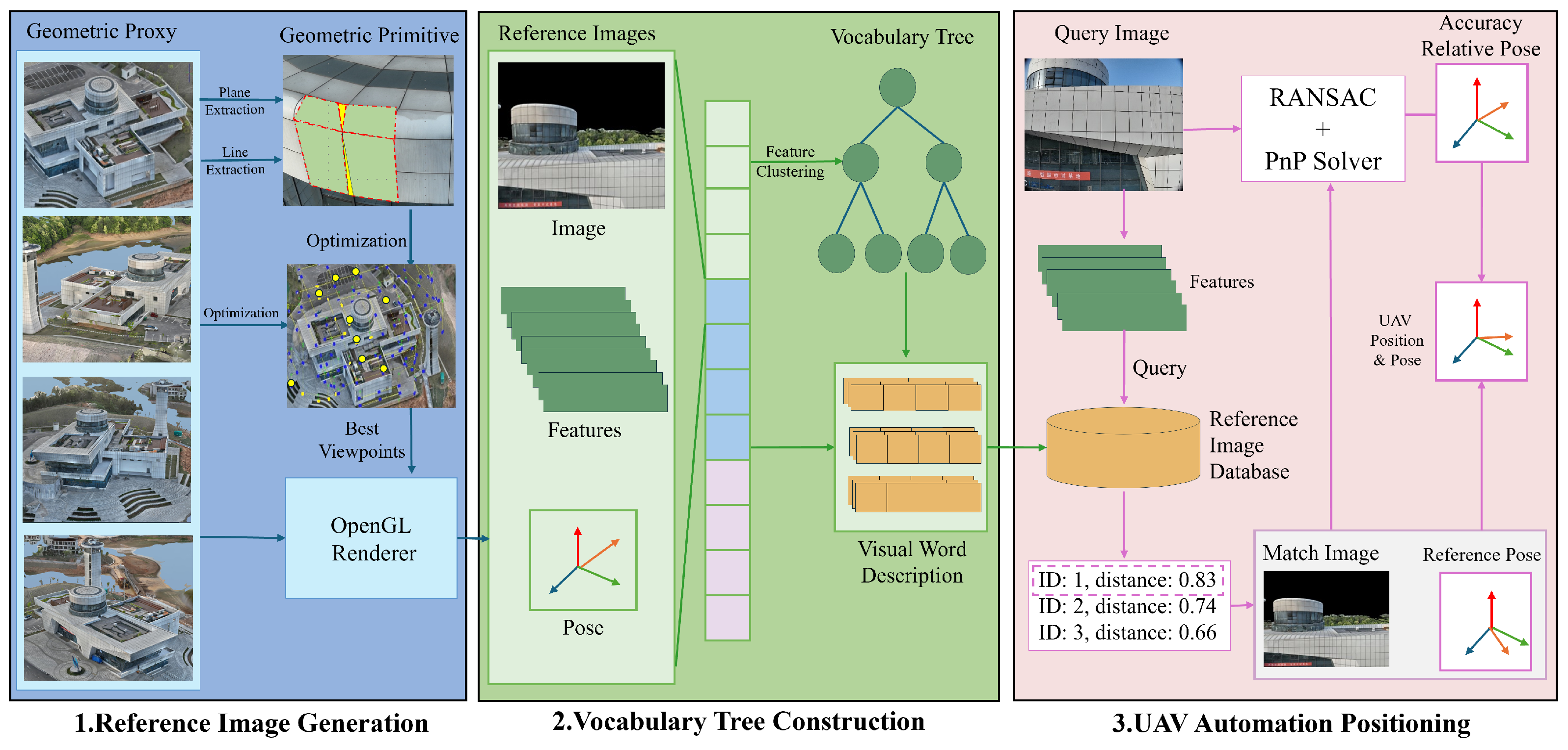
• In the viewpoint optimization stage, the method divides the 3D scene surface into geometric primitives (points, lines, polygons) and leverages plane consistency and overlap between adjacent viewpoints to frame it as an overlap optimization problem. The iterative optimization ensures complete scene coverage with minimal redundancy.
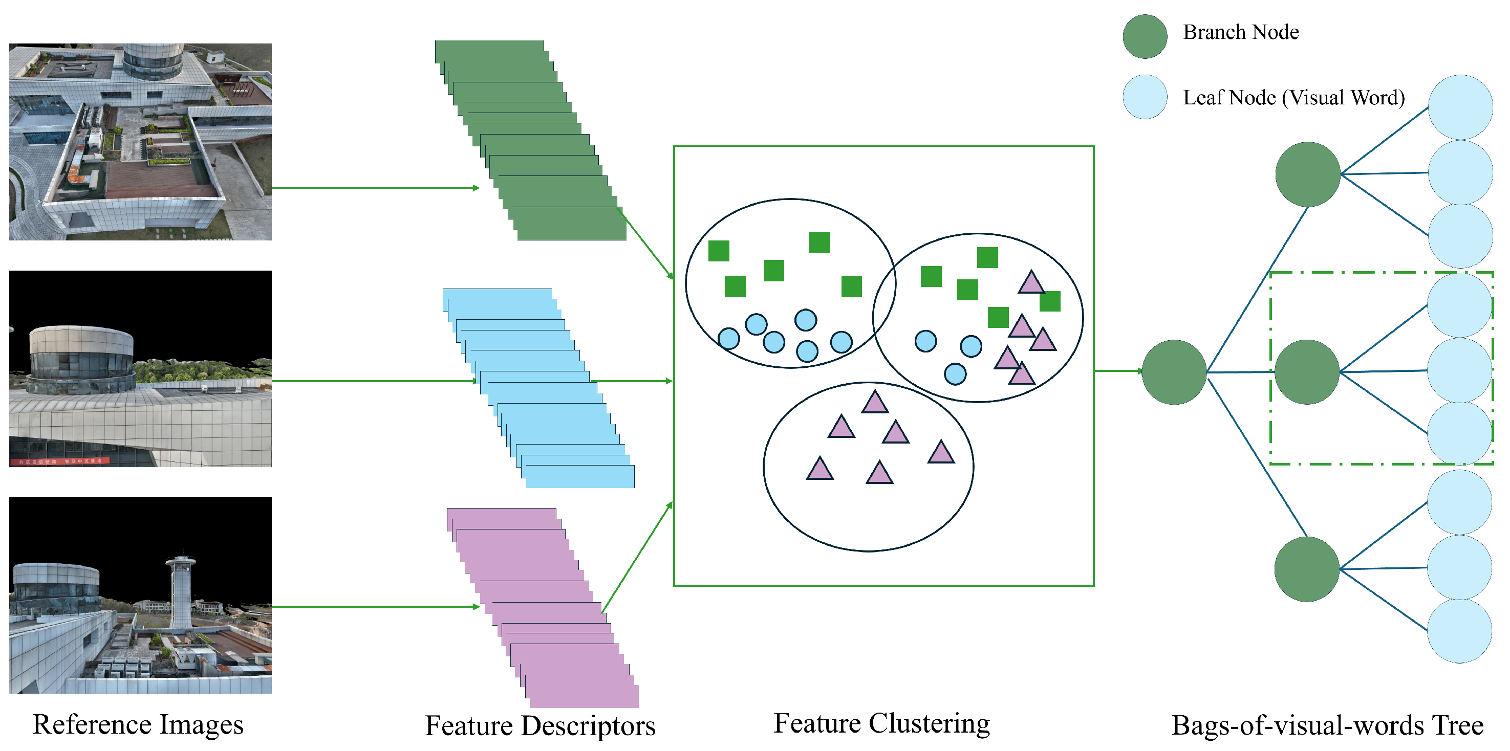
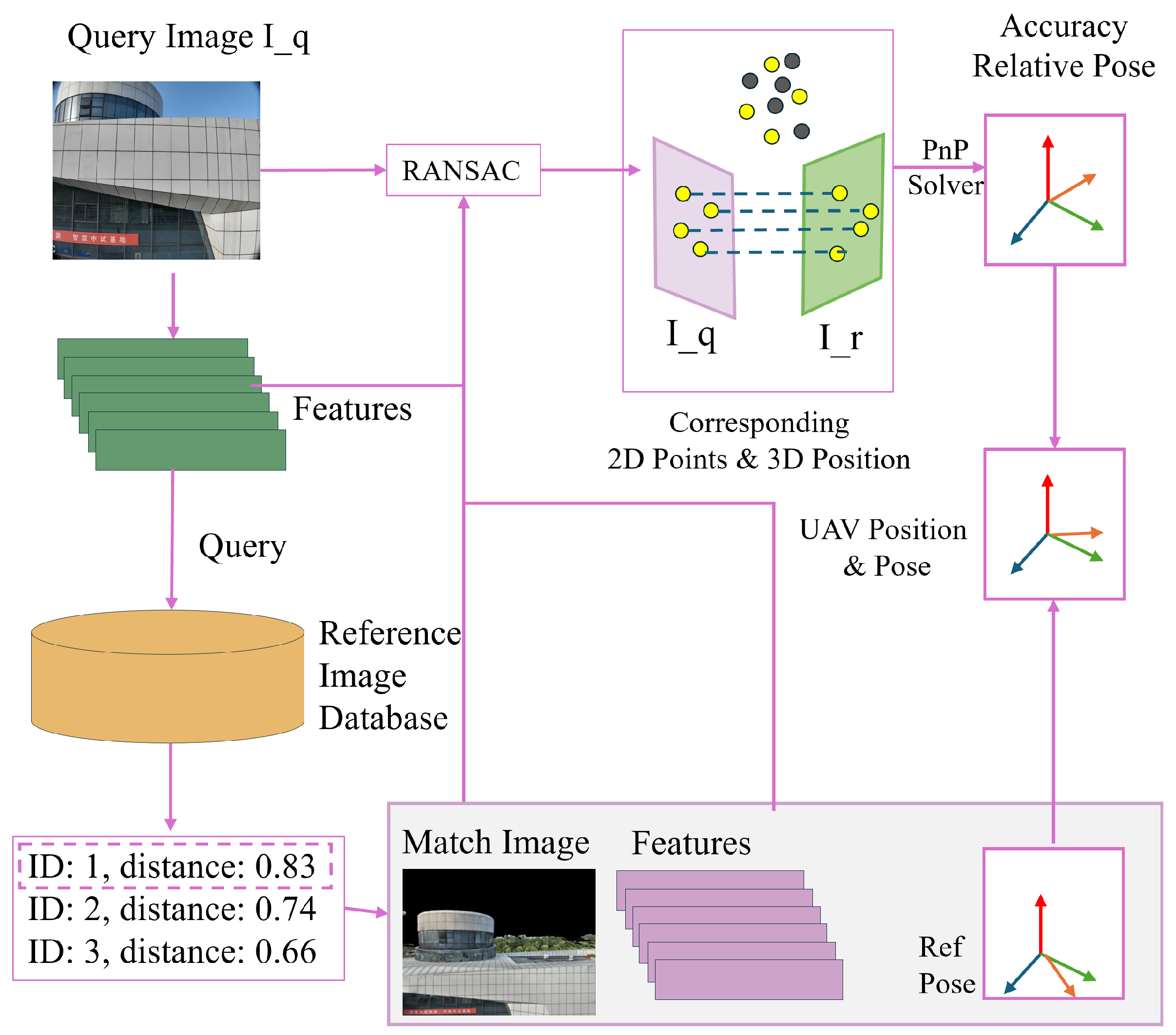
• Inspired by multi-branch tree search [16,17], the method uses a reference image bag-of-words tree to speed up image matching, clustering feature descriptors via K-Means. The tree structure aids in efficient query matching, with Random Sample Consensus (RANSAC) refining matches and the PnP algorithm estimating the drone’s six-DoF pose for fast, GNSS-free localization. The experimental results show the superiority of BoW reference image retrieval pipeline in positioning accuracy and latency.

The method requires the presence of features in the scene, and is suitable for complex urban environments. Subsequently, the proposed method needs further adjustments for environments where features are scarce or time-varying, such as snow-covered areas or off-shore oceans. The scalability of the method under extreme conditions, such as night-time or foggy weather, as well as multi-modal sensor fusion solutions, will be discussed in detail in Section 4.3.3.

The rest of this paper is organized as follows. Section 2 reviews the current research status. Section 3 presents the viewpoint optimization and bag-of-words tree construction methods. Section 4 provides the data preparation and experimental results using reference and real images from remote sensing datasets, and makes discussions for the proposed method. Finally, Section 5 concludes the paper.

2. Related Work

Drone spatial positioning relies on high-precision GNSS and INS to obtain precise positions such as latitude, longitude, and altitude. This ensures the four core functions of accurate flight control, safety assurance, mission execution, and collaboration, as well as data collection. These functions play a critical role in fields such as complex terrain exploration, emergency rescue positioning, power inspection, ecological monitoring, tracking, and smart city management, thereby enhancing overall drone operational efficiency and application value [18].

2.1. Autonomous Drone Positioning

The methods for drone autonomous positioning mainly include vision-based methods, INS-based methods, visual odometry, and hybrid approaches. Vision-based methods utilize sensors such as radars and cameras to capture external environments, followed by matching with an internal image database or map. Due to the comprehensive coverage of high-altitude reference data such as satellite and aerial imagery, most studies use geotagged satellite imagery as the reference for cross-view geographic positioning. Many works focus on cross-view matching between ground-level and satellite views. Specifically, Zhu et al. (Vigor) [7] questioned the concept of perfect one-to-one matching data pairs, introducing the idea of beyond one-to-one retrieval in ground-to-satellite matching. The University 1652 dataset [8] was the first to incorporate the drone perspective into a cross-view dataset, focusing on a target university building. Although the drone perspective can serve as a retrieval target, the task of geographic positioning remains unachieved. GeoCLIP [9] uses a Contrastive Language Image Pre-Training (CLIP)-inspired GNSS alignment between geographic locations and images, modeling the Earth as a continuous function for GNSS encoding to determine the geographic region of an image; however, it cannot obtain precise locations and poses of images. On the dataset side, Zhu et al. [10] proposed the SUES-200 cross-view dataset, which includes aerial images captured by drones at different heights and in different scenes. Ji et al. [11] constructed the GTA-UAV dataset based on the Grand Theft Auto (GTA) 5 game, containing images from various altitudes, drone angles, scenes, and targets, and developed a contrastive learning method for positioning. Due to high flight costs and the limited diversity in simulation, there remains a restriction in capturing diverse viewpoints and altitudes, making it difficult to transfer to other scenes. Ye et al. [13] constructed the AnvVisLoc dataset, which includes low-altitude orthophotos covering large areas. Xu et al. [14] proposed a large-scale dataset called UAV-VisLoc to facilitate visual positioning for drones. Cui et al. [15] divided the real-world 3D model into image and 3D point cloud datasets according to a predefined format; subsequently, real-time image capture is performed using a monocular camera mounted on the drone, followed by initial position estimation through image matching algorithms. Then, the corresponding true scene 3D point cloud data is extracted from the obtained image matching results. Finally, the point clouds reconstructed from the images are matched with the true scene 3D point cloud, and a pose estimation algorithm is applied to obtain the drone’s positioning coordinates. Ref. [18] proposed a rendering-to-localization pipeline specifically tailored for thermal image localization, which is used for registration and localization between thermal image models and 3D models.

2.2. Synthesis of Reference Images

Shan, Q. et al. [19], Sibbing et al. [20] and Shan et al. [21] rendered novel views from laser scans and multi-view stereo point clouds, demonstrating that Scale Invariant Feature Transform (SIFT) [22] feature matching between similarly posed rendered images and real images is achievable. Aubry and Russell [23] learned to match features between paintings and rendered 3D models. Torii et al. [24] improved SIFT feature matching between day and night images by synthesizing views from similar viewpoints (using depth maps). Zhang et al. [25] used view synthesis to improve pose accuracy and generated reference poses for long-term localization. Liu et al. [26] used view synthesis for the change detection of linear targets. By establishing the 2D–3D geodetic relationship between a single observation image and its corresponding 3D scene, more precise positional information can be obtained from the image. This relationship allows the transfer of depth information from a 3D model to the observation image, facilitating precise geometric change measurement for specific planar targets.

2.3. Drone Reference Image to 3D Scene Localization Solving

Common methods for drone image and 3D scene localization are based on feature matching, where correspondences are established by the similarity between feature descriptors. Wang et al. [27] utilized the SIFT feature matching algorithm to effectively find corresponding feature points between drone images and a 3D model in texture-rich scenes, thereby calculating the image position and pose in the 3D scene. This method possesses some robustness to changes in illumination, scale, and rotation, though it is computationally intensive and prone to matching errors in regions with similar textures. Liu et al. [26] established a geometric mapping between the drone images and the 3D scene model, mapping the geometric variations in the images into a 3D coordinate space with depth information to achieve precise quantification of changes for planar targets. SuperGlue [28] employs Graph Neural Networks (GNN) for feature attention and uses Sinkhorn for matching. In contrast, TransforMatcher [29] performs global-to-local matching through attention-based mechanisms, thereby achieving accurate matching and localization. Additionally, numerous studies focus on enhancing matching robustness by considering feature variance [30,31]. OnePose++ [32] adopts a multi-modal method to match point clouds with images. Another proposed alternative is to directly regress the pose parameters, such as CamNet [33]; Matteo et al. [34] proposed the 6DGS method, which estimates the camera pose by selecting a bundle of rays (radiant elliptical units) projected from the ellipsoidal surface and learning attention maps to output the ray/image pixel correspondences (based on DINOv2).

3. Method

In this section, a method is proposed for the autonomous positioning in finely detailed 3D scenes for drone navigation. The proposed method starts with a heuristic viewpoint generation mechanism that selects optimal coverage viewpoints in the 3D scene based on geometric primitives, minimizing redundancy while maintaining visual integrity. The reference images are then organized using a BoW tree for fast image-to-image retrieval, and the Perspective-n-Point (PnP) algorithm is utilized to solve drone’s detail pose and position. The workflow is illustrated in Figure 1.

Our method requires an initial geometric proxy to generate synthetic images to ensure accurate drone positioning. Typical geometric proxies comprise point clouds, digital elevation models (DEMs), 2.5D coarse models, building information models (BIMs), and 3D meshes reconstructed via oblique photogrammetry. To guarantee the quality of synthesis images, we adopt the 3D mesh as the geometric proxy.

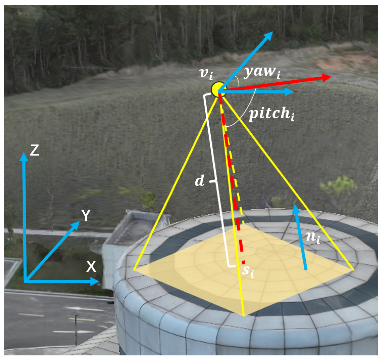
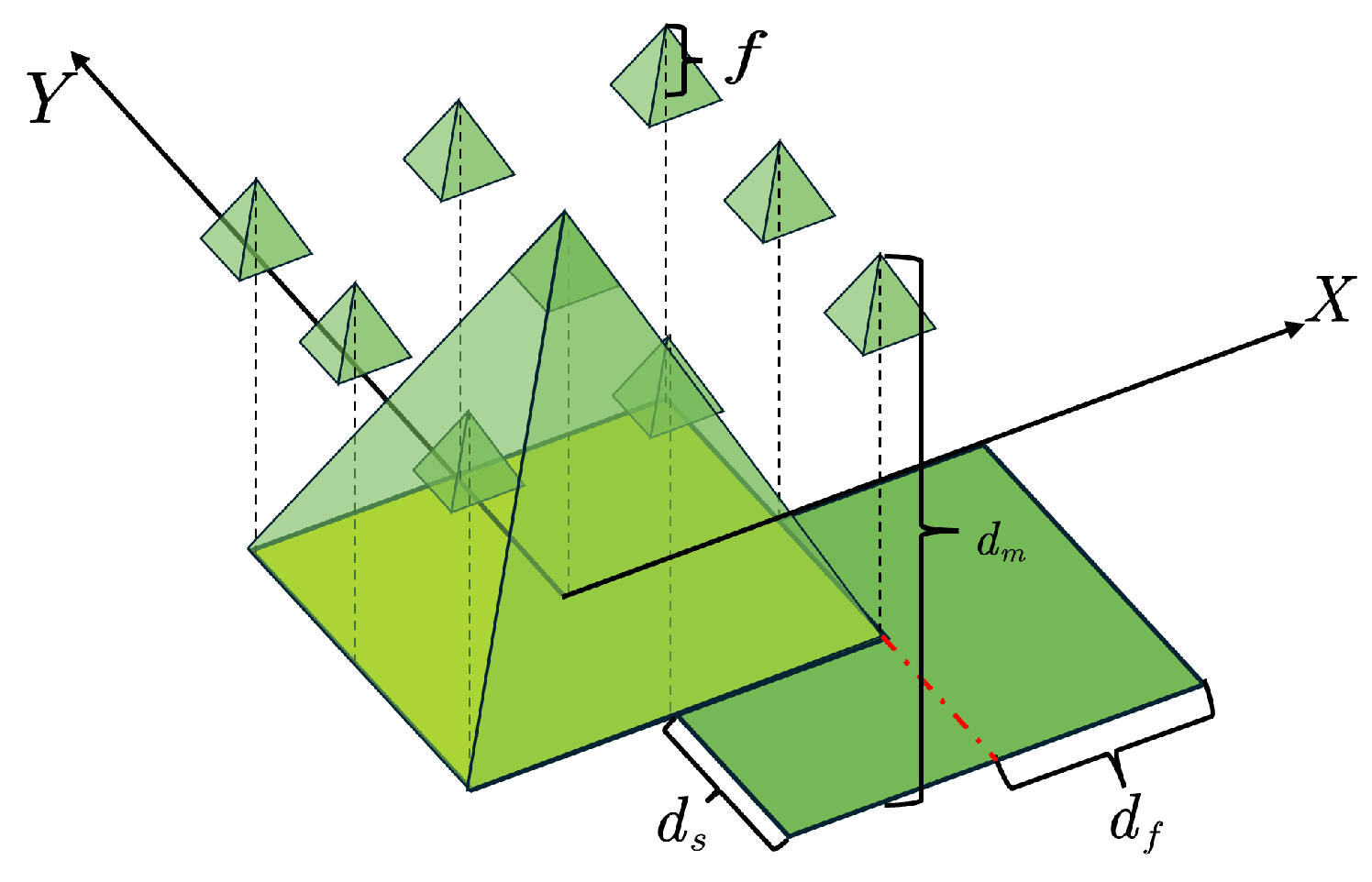
3.1. Heuristic Generation of Optimal Coverage Viewpoints

The optimal coverage viewpoints refer to a set of viewpoints that can effectively cover the scene with low redundancy. The quantification of scene coverage will be discussed later. Observing the target scene from optimal coverage viewpoints helps reduce the size of the reference image set and decreases the time required for building the visual tree index and performing image retrieval queries.

Inspired by the view generation methods in [35], we use the refined 3D surface mesh and the geometric primitives of the 3D surface mesh, including point, line, and polygon primitives, to heuristically generate the optimal coverage viewpoints. Assume the 3D model of the scene, S, is composed of several geometric primitives $p_1,p_2,\dots ,p_k$, i.e.,

$$S=\bigcup _{i=1}^k{p}_i.$$

(1)

First, using plane extraction and segmentation methods, the triangular meshes belonging to the same plane are segmented into several polygons. Then, along the boundaries of these polygons, m polygonal geometric primitives $p_1,p_2,\dots ,p_m$ are segmented from S; due to the sampling accuracy of the 3D surface mesh, the boundaries of the polygons are typically not smooth. By obtaining the line segments of the intersecting polygon boundaries, n line segment primitives $p_{m+1},\dots ,p_{m+n}$ can be obtained. An example of some geometric primitives in the geometry proxy is shown in Figure 2. Because real scenes often include small curved surfaces, smaller polygons are split into point primitives for processing.

An initial set of viewpoints, $V_0$, is generated from the 3D model S. Typically, many more sampling points are generated on the geometric proxy surface. For any sampling point $s_i$ on S, denote its normal as ${\mathit{n}}_i$ and let $d_i$ be the perpendicular distance from the drone to the plane on which this point lies. According to the orthographic projection model, the virtual viewpoint $v_i$ is given by the following:

$$v_i=s_i+d_i·{\mathit{n}}_i.$$

(2)

The pitch and heading angles of the drone can be expressed as follows:

$$\begin{array}{cc}\hfill R_1& =Rod\left(sigh{t}_1,sigh{t}_2\right)\hfill \\ \hfill R_2& =Rod\left(R_1\ast y_1,sigh{t}_2\ast Z\right)\hfill \\ \hfill yaw,pitch,roll& =angledecomposition\left(R_2\times R_1\right),roll\equiv 0\hfill \end{array}$$

(3)

The initial viewpoints only ensure that the drone can cover the sampled points on the 3D model surface; however, redundant imaging may occur, resulting in a larger reference image database and increasing the average positioning query time. To obtain the optimal coverage viewpoints, the initial viewpoint set $V_0$ needs to be adjusted and optimized. Inspired by the viewpoint quality evaluation methods in 3D reconstruction [35], we use the following metric to evaluate the coverage of a geometric primitive $p_i$ by the viewpoint set V (with $\left|V\right|\ge 2$), as shown in Figure 3.

$$C\left(p_i^{\prime },V\right)=\sum _{t\in p_i^{\prime }}\sum _{u,v\in V}f\left(t,u\right)f\left(t,p\right)c\left(t,u,v\right),$$

(4)

where

$$f\left(p,u\right)=\left\{\begin{array}{cc}1,\hfill & \mathrm{if}u\mathrm{can}\mathrm{see}p,\hfill \\ 0,\hfill & \mathrm{if}u\mathrm{cannot}\mathrm{see}p,\hfill \end{array}\right.$$

(5)

and

$$c\left(p,u,v\right)=w_1\left(\alpha \right)w_2\left(d\right)w_3\left(\alpha \right)cos\theta ,$$

(6)

which serves to evaluate the coverage of p by viewpoints u and v. Here, $\alpha$ is the parallax angle from viewpoints u and v observing p, d is the minimum distance from the two viewpoints to p, and $\theta$ is the minimum observation angle of p from u and v. The functions $w_1,w_2,w_3$ are given by the following:

$$w_1\left(\alpha \right)={\displaystyle \frac{1}{1+exp\left(-32\alpha +2\pi \right)}},$$

(7)

$$w_2\left(d\right)=1-min\left({\displaystyle \frac{d}{d_t}},1\right),$$

(8)

$$w_3\left(\alpha \right)=1-{\displaystyle \frac{1}{1+exp\left(-8\alpha +2\pi \right)}}.$$

(9)

According to [35], the value of the coverage C should be between 1.3 and 5 to achieve the optimal reference image effect. The coverage of the geometric primitive can be considered sufficient when all three rays observe the same point at an angle of 15 degrees, which leads to a minimum threshold of approximately 1.30. Additionally, when C exceeds 5, the Spearman correlation between the coverage and the accuracy of the geometric primitive’s sample point decreases significantly. If C exceeds 5, it indicates redundant viewpoints in the set V. The objective function $O\left(V\right)$ is defined as follows:

$$O\left(V\right)=\sum _{i=1}^{m+n}\left[C\left(p_i^{\prime },V\right)-1.3\right]+\sum _{i=m+n+1}^k\left[C\left(p_i^{\prime },V\right)-1.3\right].$$

(10)

Ref. [35] presents a method to determine the optimal coverage viewpoints without multiple iterations over viewpoints. Compared to traditional iterative methods, this approach fully exploits the consistency of the normals of planar polygons and line primitives, as well as the overlap between images captured from adjacent viewpoints, transforming the viewpoint optimization into an overlap optimization problem to be solved iteratively. Furthermore, it considers the coverage of minor objects for additional optimization, resulting in favorable time complexity.

As shown in Figure 4, let the virtual orthographic viewpoint of a point t on a planar or line segment geometric primitive p be u, which can be calculated via a formula and transformed into the local coordinate system of u. Suppose the drone image has along-track and cross-track overlaps denoted as A and B; the optimization objective becomes

$$A,B=argmin\sum _{t\in S}\left[C\left(t,V\left(A,B\right)\right)-1.3\right],\mathrm{s}.\mathrm{t}.C>1.3,$$

(11)

$$V\left(A,B\right)=\left\{v_i|\begin{array}{c}vx\in \left\{-d_f,0,d_f\right\}\hfill \\ vy\in \left\{-d_s,0,d_s\right\}\hfill \\ vz=d_m\hfill \end{array}\right\},$$

(12)

$$p=\left\{t_i|\begin{array}{c}sx\in \left\{-0.5d_f,0,0.5d_f\right\}\hfill \\ sy\in \left\{-0.5d_s,0,0.5d_s\right\}\hfill \\ sz=0\hfill \end{array}\right\},$$

(13)

where

$$d_s=(1-A)·H·\mathrm{GSD},$$

(14)

$$d_f=(1-B)·W·\mathrm{GSD},$$

(15)

$$d_m=f·\mathrm{GSD}.$$

(16)

Here, GSD (Ground Sample Distance) refers to the length on the ground corresponding to one pixel, in units of centimeters per pixel (cm/pixel).

It should be noted that only the polygon and line geometric primitives cannot cover the entire scene. Typically, the scene may contain trees, bushes, and other fine objects; however, accounting for too many fine objects increases the number of generated viewpoints, which is not conducive to the subsequent generation of reference images. Therefore, we weight the area $A_s$ corresponding to the region represented by the point geometric primitive to obtain the following optimization objective:

$$v_i=argmax\sum _{s\in p^{\prime }}\left[exp\left(1.3-H\left(s,V\right)\right)-1\right]·A_s.$$

(17)

In this way, by assessing the coverage of the scene by the drone, we obtain the optimal set of coverage viewpoints V. Later, this set V will be used to generate a bag-of-words tree for the reference images.

3.2. Bag-of-Words Tree for Reference Images

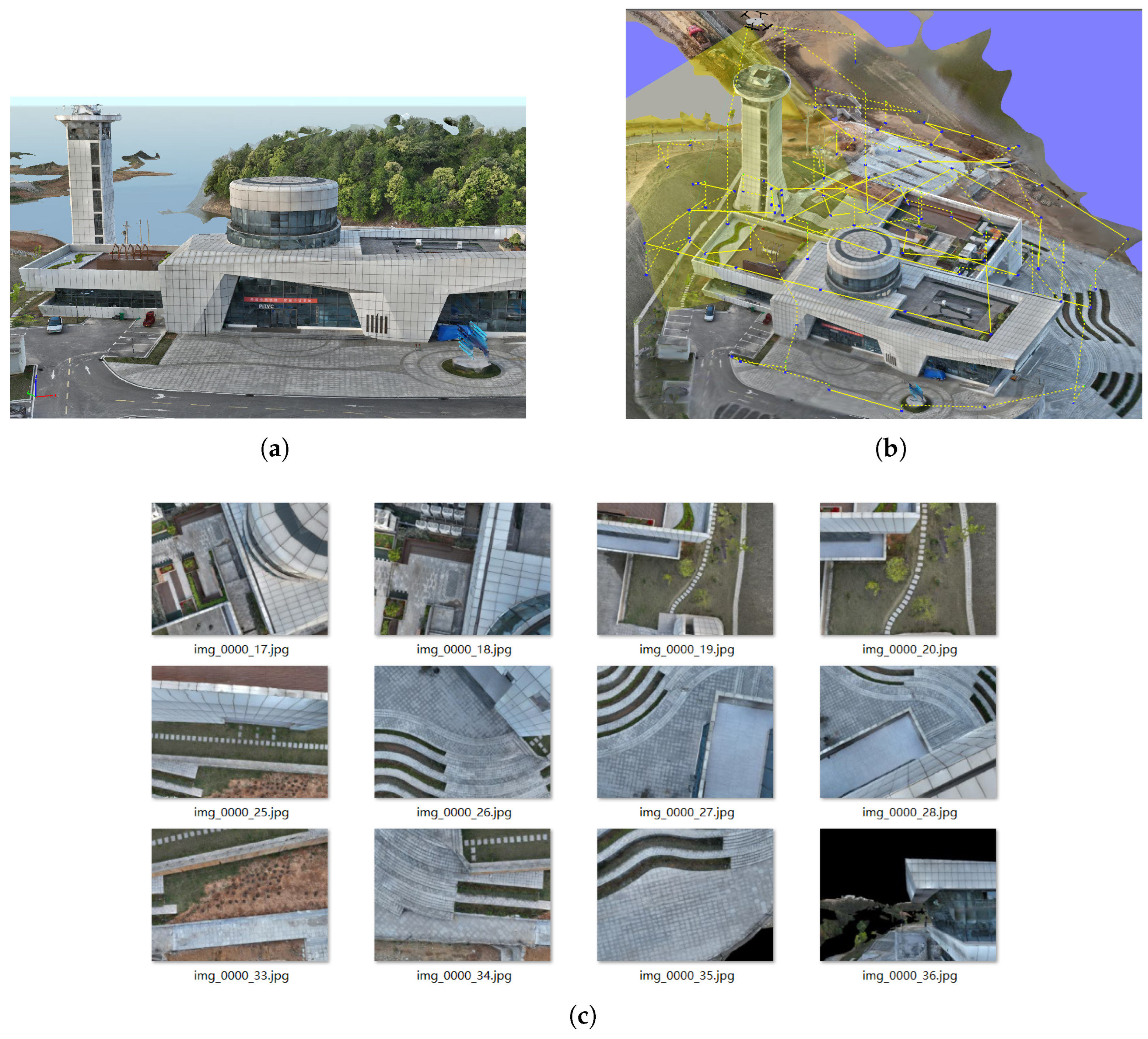
3.2.1. Generation of Reference Images

Previous research has shown that the rendered images of textured 3D models from given viewpoints can not only achieve feature matching with real observation images but can also effectively reduce the influence of lighting variations on the registration between reference and observation images, thereby improving autonomous positioning accuracy. Using the optimal coverage viewpoint set V generated in Section 3.1 and the 3D digital model S, we can generate virtual observation images of S from a viewpoint $v\in V$ with a given pose R. By employing a process similar to the one in Section 3.1 to generate the optimal viewpoint set V, the virtual observation images, captured from different poses covering the 3D digital model S, can serve as references for the drone’s autonomous positioning. We call these images the reference images. Using an OpenGL renderer, the 3D digital model S, the optimal viewpoint set V, and a set of poses T are used to generate the reference images. According to the OpenGL rendering pipeline (as indicated in the literature, reference placeholder), the imaging equation of a reference image can be expressed as follows:

$$\left(\begin{array}{c}x\\ y\\ 1\end{array}\right)=\mathbf{PVM}\left(\begin{array}{c}{x}_s\\ y_s\\ z_s\\ 1\end{array}\right)=\mathbf{P}\left(\begin{array}{cc}\mathit{R}& -\mathit{R}v\\ 0& 1\end{array}\right){\mathbf{I}}_{4\times 4}\left(\begin{array}{c}{x}_s\\ y_s\\ z_s\\ 1\end{array}\right),$$

(18)

where v is the viewpoint, $\mathit{R}$ is the drone’s pose at viewpoint v, and $\mathbf{P}$ is the projection matrix. OpenGL maps the above coordinates to screen coordinates through perspective division and viewport transformation, saving the pixel values in the render buffer to the disk to obtain the reference image observed at viewpoint v with pose $(R,t)$. By iterating over the optimal viewpoint set V and adjusting the drone’s pose, a large number of reference images $\mathbb{L}$ can be quickly generated.

3.2.2. Image Feature Extraction and Matching

Common image feature extraction algorithms include both traditional and learning-based methods. Traditional feature extraction descriptors include SIFT (Scale Invariant Feature Transform) [22], SURF (Speeded Up Robust Features) [36], and ORB (Oriented FAST and Rotated BRIEF) [37]. Among them, SIFT has scale, rotation, viewpoint, and brightness invariance, but it has high computational complexity. SURF uses a 64-dimensional Haar wavelet estimate to construct descriptors, while the ORB algorithm calculates orientation using the centroid method and adopts a learning-based binary descriptor. In recent years, some learning-based feature descriptors have been widely used, such as SuperPoint [38] and D2-Net [39]. However, learning-based descriptors generally rely on large, manually annotated datasets (>10,000 images), which hinders rapid deployment across diverse environments. Therefore, this paper still chooses traditional feature extraction descriptors and will compare the positioning accuracy and speed of these three descriptors in the experimental section.

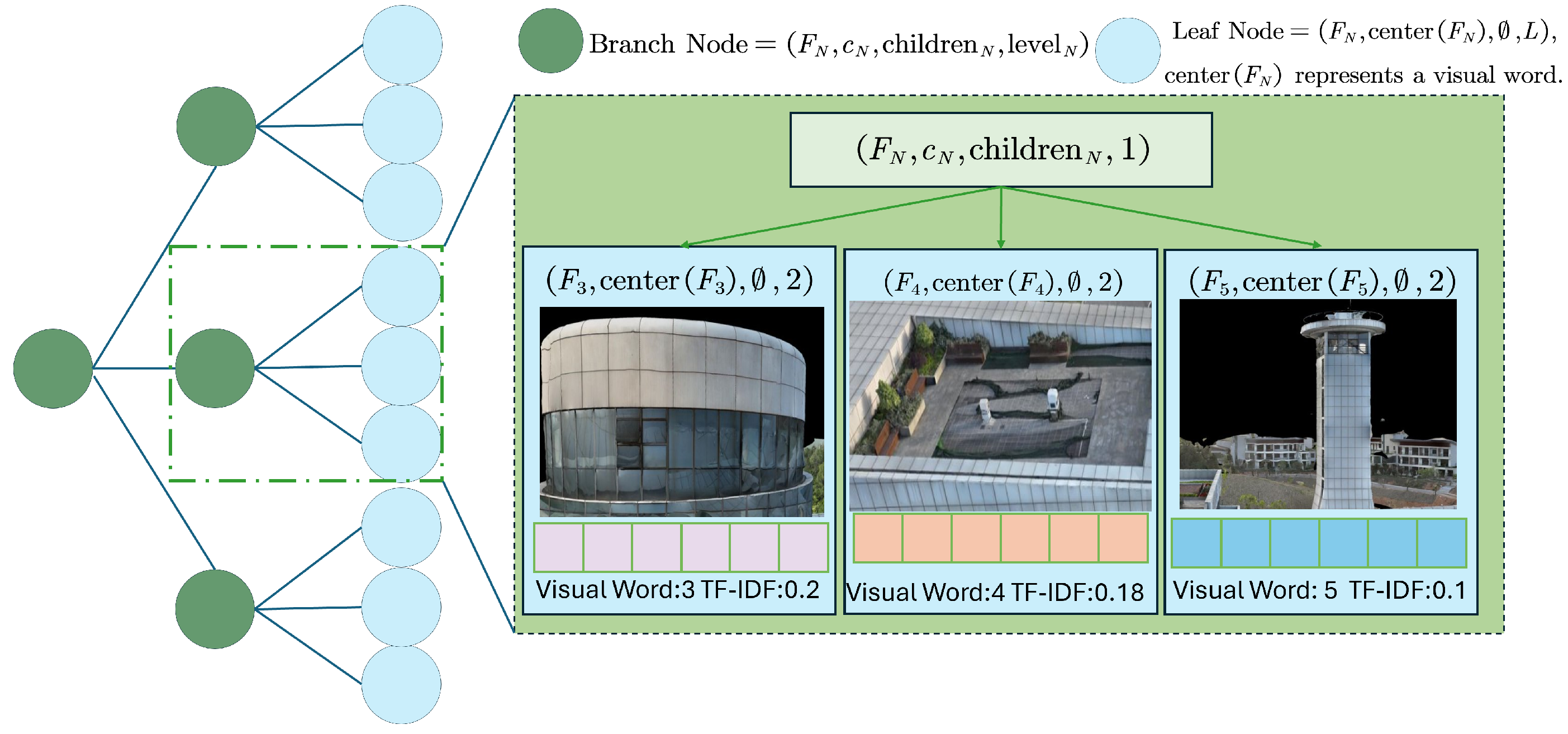
3.2.3. Construction of the Bag-of-Words Tree for Reference Images

Inspired by multi-branch tree search, a bag-of-words tree data structure [16,17] was proposed to improve the naive bag-of-words model [40]. This data structure first compresses similar visual feature descriptors using the K-Means clustering algorithm [41], and then organizes the feature descriptors into a K-ary tree, where the leaf nodes represent the visual word representation of the reference images. The construction of a visual bag-of-words tree can be illustrated as in Figure 5.

For the generated reference images $\mathbb{L}=\{I_1,I_2,\dots ,I_r\}\in {\mathbb{R}}^{r\times H\times W}$, an image feature extraction algorithm (e.g., ORB) is used to extract the feature descriptors $F\left(\mathbb{L}\right)={\bigcup }_{i=1}^{r}F\left(I_i\right)=\{F_1,F_2,\dots ,F_m\}$, where

$$F\left(I_r\right)=\{d_{r,1},\dots ,d_{r,n_r}\},$$

(19)

and m is the total number of feature descriptors. Let the number of layers in the bag-of-words tree be L, and let each node of the tree be represented as a quadruple:

$$\mathcal{N}=\left(F_N,c_N,{\mathrm{children}}_N,{\mathrm{level}}_N\right),$$

(20)

where $F_N$ is the set of descriptors represented by the node, $c_N$ is the cluster center coordinate, ${\mathrm{children}}_N$ is the set of child nodes of $\mathcal{N}$ (empty if $\mathcal{N}$ is a leaf node), and ${\mathrm{level}}_N$ is the level of the node in the tree. The construction process of the bag-of-words tree can be described as follows:

$$T\left(F,\mathrm{level}\right)=\left\{\begin{array}{cc}\left(F,\mathrm{center}\left(F\right),\varnothing ,\mathrm{level}\right),\hfill & \mathrm{if}\mathrm{level}=L,\hfill \\ \left(F,\mathit{c},\left\{T\left(F_j,\mathrm{level}+1\right)\right\},\mathrm{level}\right),\hfill & \mathrm{otherwise},j\in \{1,\dots ,k\},\hfill \end{array}\right.$$

(21)

where $F={\bigcup }_{j=1}^k{F}_j$ and $\mathit{c}=\{c_1,\dots ,c_k\}$ represent the sets of feature descriptors and the corresponding centers obtained by clustering F into k clusters using the K-Means algorithm, and $\mathrm{center}\left(F\right)$ is the center of F. In the constructed optimal bag-of-words tree for the reference images, the total number of leaf nodes is $k^L$. For any leaf node $\mathcal{N}$, a unique node ID $\mathcal{W}\left(d\right)\in \{0,\dots ,k^L-1\}$ can be determined. For the feature descriptors of an image I, i.e., for all $d\in F\left(I\right)=\{d_1,d_2,\dots ,d_n\}$, let the leaf node retrieved by traversing the K-ary tree be $\mathcal{N}\left(d\right)$. We use the node ID $\mathcal{W}\left(d\right)$ of $\mathcal{N}\left(d\right)$ as the visual word representation of d. By mapping the feature descriptors of the image I accordingly and counting the histogram of visual words, the bag-of-words representation of the image I is obtained:

$$H:{\mathbb{R}}^{H\times W}\to {\mathbb{R}}^{K^L},H\left(I\right)=\{h_0,h_1,\dots ,h_{K^L-1}\},$$

(22)

where $h_i,i\in \{0,\dots ,k^L-1\}$ denotes the frequency of visual word i.

3.2.4. Node Weight Assignment

Compared with the traditional visual bag-of-words model, the visual bag-of-words tree offers a stronger representation of the image database; however, different visual words carry different weights in an image’s word representation. The Term Frequency-Inverse Document Frequency (TF-IDF) measure is used to describe the weight of a visual word. The idea is that if a visual word appears with high frequency in one image but rarely in others, it is considered more discriminative; if it appears frequently in many images, it is considered generic. The TF-IDF for visual word i is computed as follows:

$$g\left(i\right)={\displaystyle \frac{n_i}{{\sum }_{0\le j\le k^L-1}{n}_j}}·log\left({\displaystyle \frac{\left|\mathbb{L}\right|}{|{\mathbb{L}}_i|+1}}\right),$$

(23)

where $n_i$ is the number of occurrences of visual word i in the current image, and ${\mathbb{L}}_i$ denotes the set of reference images containing visual word i. $\left|\mathbb{L}\right|$ represents the total number of images in set $\mathbb{L}$, while $|{\mathbb{L}}_i|$ denotes the total number of images in subset $L_i$. By using g instead of h, the bag-of-words representation of the image I becomes

$$G:{\mathbb{R}}^{H\times W}\to {\mathbb{R}}^{K^L},G\left(I\right)=\{g_0,g_1,\dots ,g_{K^L-1}\}.$$

(24)

For the purpose of facilitating the subsequent search for the reference image I, the bag-of-words tree T is built by calculating the TF-IDF to obtain the set of reference images containing the visual words observed in the query image, thereby accelerating the localization process. Figure 6 shows an example of a visual bag-of-words tree for a certain scenario.

3.3. Autonomous Drone Positioning Based on the Reference Image Bag-of-Words Tree

For a drone at the current position $\mathit{x}$ observing an image $I_x$ with pose ${\mathit{R}}_x,t_x$, we first extract the feature descriptors $F\left(I_x\right)=\{d_{x1},\dots ,d_{xn}\}$ in the same manner as in Section 3.2.2. Starting from the root node of the bag-of-words tree T, for the k cluster centers $\mathit{c}=\{c_1,c_2,\dots ,c_k\}$, the distance between each input descriptor $d_{x_i}$ and each $c_j\in \mathit{c}$ is computed as $dis{t}_j=d\left(d_{x_i},c_j\right)$ for $j\in \{1,2,\dots ,k\}$. The branch corresponding to the minimum distance is selected, and the process repeats until it iterates L times, at which point the visual word representation $\mathcal{W}\left(d_{xi}\right)$ is obtained. In turn, the bag-of-words representation $G\left(I_x\right)$ of the image $I_x$ is formed. Subsequently, an appropriate distance metric is used to measure the similarity between the bag-of-words representations of the image $I_x$ and the reference image I:

$${\mathrm{children}}_j,j=argmindis{t}_j.$$

(25)

Common distance functions include cosine similarity, $L_1$ distance, and $L_2$ distance. If the bag-of-words representations of $I_x$ and I are $G_1=G\left(I_x\right)$ and $G_2=G\left(I\right)$, respectively, then their cosine similarity, $L_1$, and $L_2$ distances are given by the following:

$$d_{cos}\left(G_1,G_2\right)=1-cos\langle G_1,G_2\rangle =1-{\displaystyle \frac{G_1·G_2}{\parallel G_1\parallel \parallel G_2\parallel }},$$

(26)

$$d_{L_1}\left(G_1,G_2\right)={\parallel G_1-G_2\parallel }_1,$$

(27)

$$d_{L_2}\left(G_1,G_2\right)={\parallel G_1-G_2\parallel }_2.$$

(28)

When the cosine distance $d_{cos}$ approaches 0, or the $L_1$ and $L_2$ distances approach 0, the bag-of-words representations of the images $I_x$ and I are considered more similar. The reference image $I_r$ can thus be derived as follows:

$$I_r=argmin\left(d\left(G_1,G_2\right)\right).$$

(29)

Then, using the previously extracted feature points from $I_x$ and I, matching feature point pairs

$$P=\left\{\{f_{x_1},f_1\},\dots ,\{f_{x_{nn}},f_{nn}\}\right\}$$

(30)

are sought. The RANSAC algorithm [42] is applied to remove incorrect matching pairs, yielding the final set of matches. By computing the positional error between the virtual image and the reference image based on the matching positions, if the error exceeds a threshold, the image coordinates of the feature points are then used to compute the current drone pose. As illustrated in the figure, let the coordinates of the reference image feature point in the world coordinate system be ${\mathcal{P}}_{\mathrm{ref},i}$, with pose ${\mathit{R}}_{\mathrm{ref}},{\mathit{t}}_{\mathrm{ref}}$, camera intrinsic matrix $\mathit{K}$, and depth $d_i$. Then we have the following:

$${\mathcal{P}}_{\mathrm{ref},i}={\mathit{R}}_{\mathrm{ref}}^{-1}\left(d_i·{\mathit{K}}^{-1}{f}_i-{\mathit{t}}_{\mathrm{ref}}\right).$$

(31)

The current drone pose $(\mathit{R},\mathit{t})$ can be expressed as the following nonlinear least squares optimization problem:

$$(\mathit{R},\mathit{t})=arg\underset{R,t}{min}\sum _{i=1}^{nn}{∥f_{xi}-{\mathit{K}}^{\prime }\left[\mathit{R}{\mathcal{P}}_{\mathrm{ref},i}+\mathit{t}\right]∥}^2.$$

(32)

This problem can be solved using the PnP algorithm [43,44], thereby obtaining the current pose of the drone. The whole positioning procedure can be described as Figure 7.

4. Experimental Results and Discussion

4.1. Experimental Settings

We utilized the DJI Mavic 3E drone to capture the Intelligent Unmanned System Testing Base of the Chibi Pilot Valley in Xianning City, Hubei Province, to obtain our 3D geometric model. For the specified test scenario, a 3D reconstruction method [35] was employed, with the geometric model’s accuracy around 0.05 m. Subsequently, 114 effective viewpoints were generated using the method in Section 3.1, and synthetic images were rendered using OpenGL. The 3D geometric model, optimal coverage viewpoints, and reference images are shown in Figure 8a, Figure 8b, and Figure 8c, respectively.

All evaluations were conducted on an Intel Core i7-14650HX CPU, RTX 4060 GPU, and Windows OS (Version 10). The proposed method uses C++ with OpenCV 4.11, EXIF 2, and TinyXML libraries. The feature extraction method used in the experiment was ORB, with 500–1000 feature points and descriptors extracted from each image. The resolution of each image is 5280 × 3956, and 100 images were tested. The reference image is obtained using the ideal pinhole camera model without distortion; however, the query images are captured using a real wide-angle lens, which introduces distortion. According to [45], the distortion of images can contribute to fewer corresponding points, so that the accuracy of position and pose might decrease according to Equation (30). The camera model is a pinhole model with distortion. The camera’s focal length, which is provided by Shenzhen Dajiang Innovation Technology Co., Ltd., Shenzhen, China, and the distortion parameters, which are estimated through camera calibration, are shown in

Table 1. Camera focal length and distortion parameters.

Focal Length	K1	K2	K3	P1	P2
33 mm	−0.11153155	0.01035897	−0.02430045	0.00011204	−0.00007903

. The images are rectified to minimize feature matching errors.

In this experiment, K is set to 10, and L is set to 5 in the visual bag-of-word tree.

4.2. Experiment Results

Since the PnP method relies on the relative position of 2D–3D point pairs to estimate the camera pose, the consistency of pose estimation mainly depends on the accuracy of the 3D points and the consistency of the 2D point pairs. The former is primarily influenced by the accuracy of the 3D geometric model, while the latter is influenced by feature extraction and feature matching methods. This section evaluates the accuracy of the reconstructed 3D geometric model, localization results, and the impact of different feature matching methods on localization accuracy.

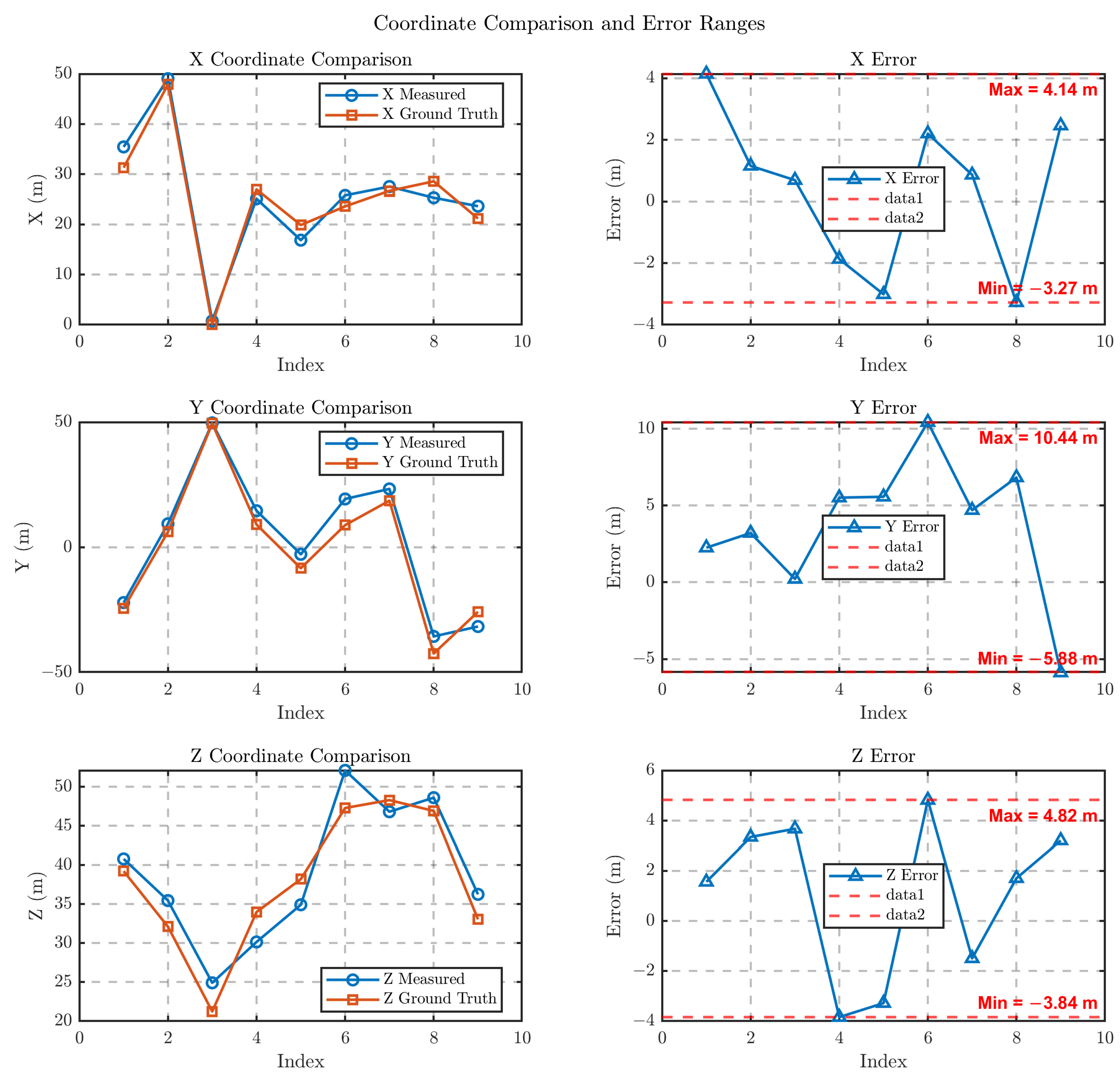
4.2.1. Accuracy of the Geometric Model

To evaluate the accuracy of the 3D geometric model, we calculate the PSNR (Peak Signal-to-Noise Ratio), SSIM (Structrual Similarity), and visualize the accuracy of the 3D model by comparing the reference images with the query images at the same shooting location.

Table 2. PSNR, SSIM, and RMSE for 3D model reference images and real captured images. (↑ higher is better; ↓ lower is better).

Metrics	PSNR ↑	SSIM ↑	RMSE ↓
Image Set I	29.84	0.5216	0.265
Image Set II	29.65	0.5359	0.276
Image Set III	29.78	0.5562	0.268
Image Set IV	29.95	0.5087	0.258
Image Set V	29.86	0.5179	0.263
Average	29.82	0.5281	0.266

shows that the PSNR values for several images are above 29, indicating that the 3D model reference image is quite close to the real captured image. SSIM values above 0.5 suggest a moderate similarity in brightness, structure, and contrast between the 3D model reference image and the real image. This similarity could be due to minor geometric transformations and differences in lighting intensity between the real and reference images. These results demonstrate that the 3D reconstruction method generates a geometric model with high accuracy, suitable for drone positioning. Figure 9 visually shows the similarity between the two sets of 3D model reference images and real captured images.

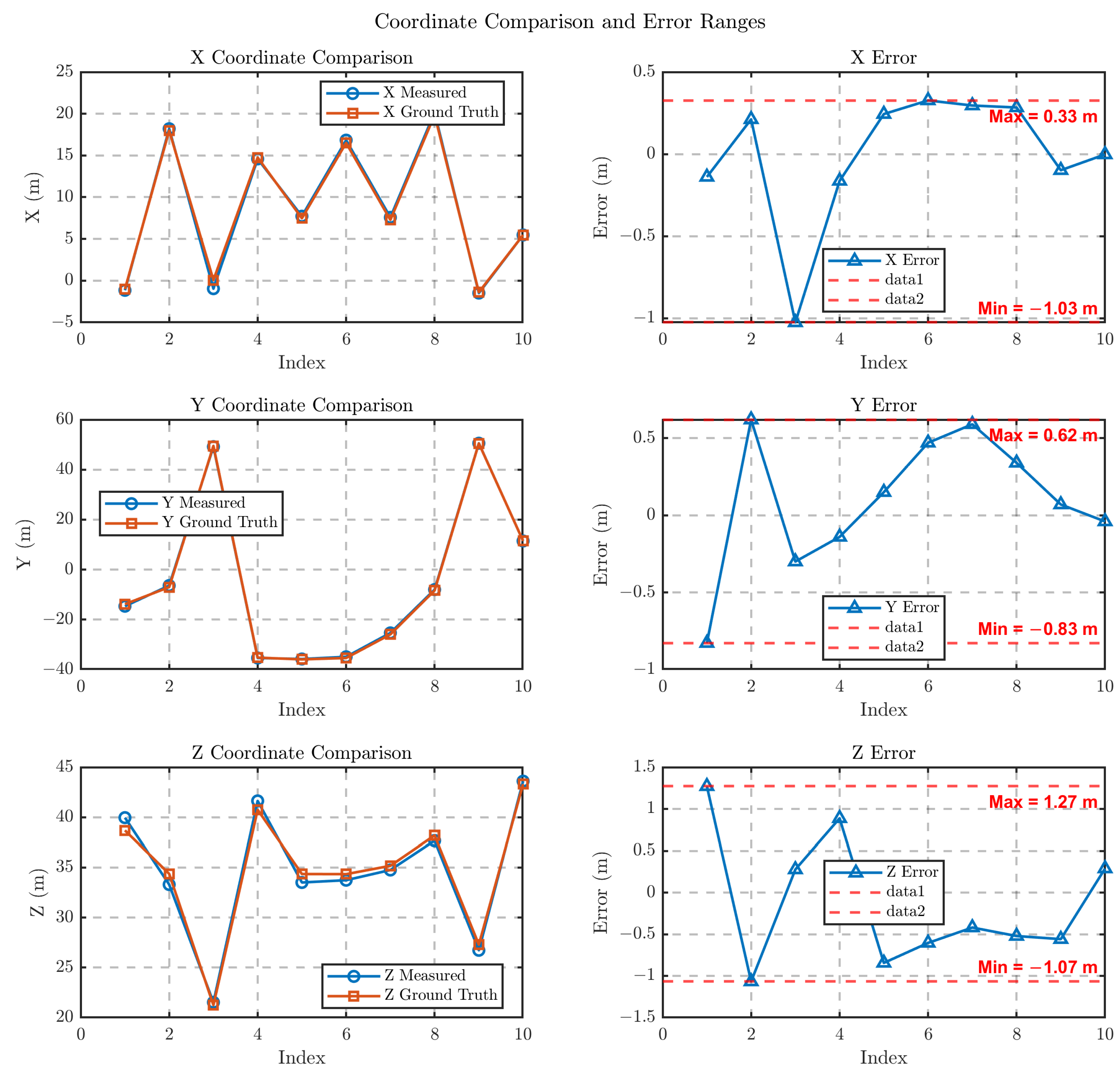
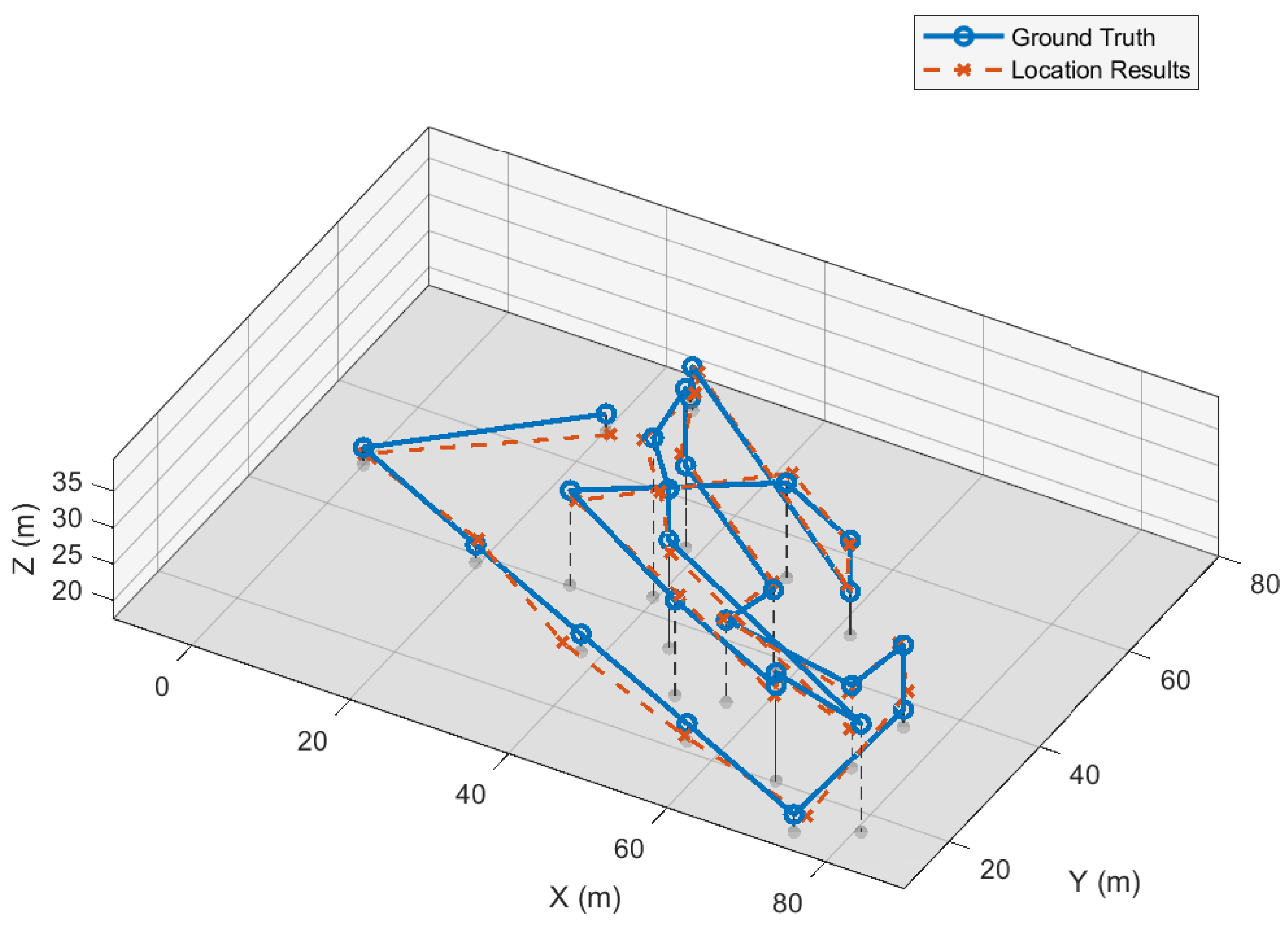
4.2.2. Localization Results in Different Poses and Position

To verify the accuracy of the proposed algorithm, the drone captures a set of photos at different locations. During the image capture process, the drone’s position is obtained using real-time dynamic carrier phase difference technology (RTK). The drone’s self-positioning coordinates are calculated in real-time using the proposed algorithm. This method allows for positioning accuracy without relying on the GNSS, achieving accuracy within 1–5 m. The RTK and proposed algorithm’s positioning coordinates and errors in the X, Y, and Z directions at different positions are plotted in Figure 10 and Figure 11.

Figure 10 plots RTK vs. our algorithm’s estimates (and their X, Y, and Z errors) when the pose discrepancy between query and reference images is small (rotation < 5°; translation < 0.5 m). In this regime, we achieve errors of less than 1 m along each Cartesian axis. Figure 11 shows the same comparison under large pose mismatches (rotation > 15° or translation > 2 m), where errors remain below 5 m per axis, though the Y-axis (East–West) occasionally exceeds 5 m—likely due to reprojection and coplanar matching limitations. We also computed the Euclidean (3D) position error and localization time in the position with a small difference between query and reference pose; the results are given in

Table 3. Spherical positioning error, rotation error, and localization time of the drone at different positions.

Position	Error (m)	Rotation Error	Localization Time (ms)
Position I	1.51	0.00060	963
Position II	1.24	0.00090	901
Position III	1.22	0.00077	709
Position IV	0.91	0.00073	1291
Position V	0.89	0.00092	862
Position VI	0.83	0.00080	1028
Position VII	0.77	0.00066	1049
Position VIII	0.69	0.00074	1023
Position IX	0.55	0.00077	835
Position X	0.29	0.00081	1023

.

We also evaluated the drone’s spherical positioning accuracy and localization time (see Table 3).

Table 3 presents the drone’s spherical positioning error, rotation error, and localization time across ten different positions, which are the same as positions shown in Figure 10. The positioning error is computed using the Euclidean distance formula, and rotation error is evaluated via the following equation:

$$RotationError={\parallel R_{gt}{R}^T-I\parallel }_2$$

(33)

where $R_{gt}$ is the ground truth rotation matrix, R is the estimated rotation matrix, and I is the identity matrix. ${\parallel ·\parallel }_2$ means L2 norm of one matrix.

The results indicate that the proposed method achieves sub-meter positioning accuracy in most cases, with the lowest positional error recorded at 0.29 m and the highest at 1.51 m. Rotation errors remain consistently low across all tested positions, generally on the order of ${10}^{-4}$. Localization times range between approximately 700 ms and 1300 ms, demonstrating the method’s capability for real-time or near real-time performance. These results indicate the reliability and efficiency of the proposed UAV localization method under the evaluated conditions.

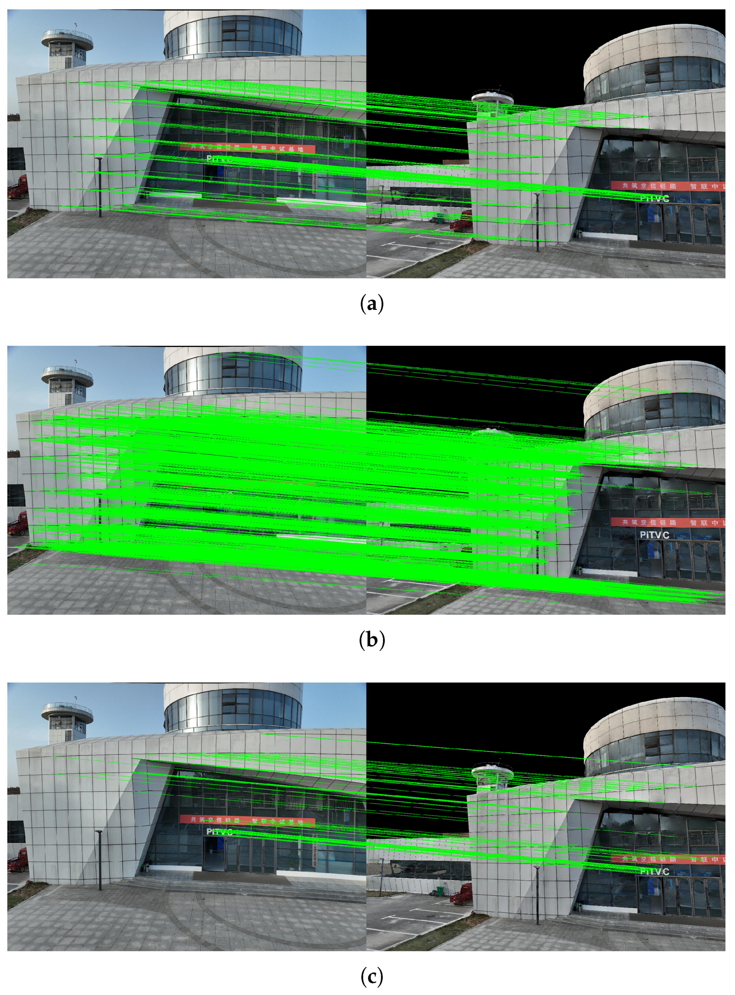
4.2.3. The Effect of Different Feature Matching

To evaluate the impact of different feature descriptors and matching methods on localization accuracy and indexing speed, this section selects three widely-used techniques: SIFT [22], SURF [37], and ORB [38]. The evaluation metrics include the maximum error, minimum error, maximum rotational error, minimum rotational error, mean error, mean rotational error, and average localization time.

Table 4. Localization performance metrics across SIFT, SURF, and ORB.

Metric	SIFT [22]	SURF [37]	ORB [38]
Max Error (m)	2.422	2.498	2.437
Min Error (m)	0.209	0.231	0.237
Max Rotational Error	0.004589	0.006195	0.003686
Min Rotational Error	0.000301	0.000174	0.000168
Mean Error (m)	0.708	0.816	0.919
Mean Rotational Error	0.001014	0.001013	0.000958
Avg. Localization Time (s)	20	35	0.75

summarizes the influence of these methods on localization accuracy and processing time. As shown in Table 4, ORB achieves relatively good localization accuracy with minimal time overhead, while SIFT delivers the best precision at the cost of longer computation time. Specifically, while SIFT utilizes high-dimensional real-valued descriptors to capture detailed scale and orientation information, this advantage comes at a higher computational expense, especially due to the larger number of feature points it generates. The extensive use of descriptors and their increased sensitivity to noise and complex textures can lead to more error-prone matches in certain scenarios, especially in environments with high texture repetition or noise. This may introduce an additional burden when computing the rotation matrix, potentially resulting in higher rotational errors compared to ORB. On the other hand, ORB, with its binary BRIEF descriptors, requires fewer computational resources, which leads to a faster matching process, though it may sometimes overlook finer details of the image. This trade-off allows ORB to maintain a balance between speed and accuracy, particularly in dynamic and resource-constrained environments. Meanwhile, SURF accelerates convolution operations using integral images but still suffers from limitations in efficiency due to the complex Haar wavelet responses and the overhead associated with medium-to-high dimensional descriptor matching.

Despite these optimizations, SURF still incurs significant time costs during descriptor generation and matching, especially when dealing with larger sets of features. The feature matching results for the three methods are illustrated in Figure 12, highlighting the trade-offs between precision, speed, and computational demands.

The reported average localization times include the duration for loading both the query and reference UAV images, which have high resolutions (5280 × 3956 pixels), thus contributing to increased overhead during image reading and descriptor computation.

4.3. Discussion

The above experimental results demonstrate the matching performance of benchmark images based on the optimal viewpoint coverage strategy. To further evaluate the performance of our method in real-time drone flight positioning, we set up a set of flight routes to assess the performance of the autonomous positioning method. The results of the autonomous positioning method are shown in the Figure 13, with a positioning error within 2 m and an angle error within 5°. This indicates the robustness of our method. This method does not require any pre-training and achieves the autonomous localization of UAVs in large-scale environments without relying on point clouds generated from images, thereby verifying the feasibility and effectiveness of the proposed UAV autonomous localization approach. This significant improvement highlights the potential of our method in a variety of real-time UAV applications, where both accuracy and efficiency are crucial. In the following sections, we delve deeper into sensitivity analysis, comparisons with other methods, and the limitations of the current approach, while also discussing future enhancements to address specific challenges in diverse operational environments.

4.3.1. Sensitivity Analysis

To analyze the impact of the number of branches K and tree depth L on the retrieval performance of a visual vocabulary tree, we configured the values of K and L based on the actual number of visual words: (5, 5), (5, 8), (5, 10), (10, 3), (10, 5), and (10, 8). The evaluation metrics included index construction time, memory usage of the index database file, average query time, and retrieval accuracy. The total number of test images is 100. Retrieval accuracy was determined by manually comparing the number of correct matches to the total number of queried images. The results are shown in

Table 5. Retrieval performance under different vocabulary tree parameters.

Parameters	Construction Time (s)	Index Memory (MB)	Average Query Time (ms)	Retrieval Accuracy (%)
K = 5, L = 5	19.85	0.925	8.355	60
K = 5, L = 8	21.02	43.495	7.177	70
K = 5, L = 10	19.23	68.670	7.694	74
K = 10, L = 3	15.16	0.268	8.025	55
K = 10, L = 5	16.70	21.683	7.898	69
K = 10, L = 8	21.59	68.168	7.814	72

.

Retrieval accuracy significantly improves with an increase in the number of leaf nodes and shows a moderate improvement with changes in the branching factor K. Query time remains relatively stable with limited sensitivity to changes in K and L, showing only minor fluctuations due to tree depth or branching variations. Construction time tends to increase with deeper trees or higher branching factors, though not always linearly. Memory usage of the index grows sharply as the number of leaf nodes increases.

We choose the shape of $K=10,L=5$ instead of $K=5,L=10$ because the latter combination has the highest index memory usage among all configurations, reaching 68.670 MB. This may pose significant challenges for deployment in resource-constrained environments. In addition, the construction time of 19.23 s is relatively long, which may become a bottleneck when processing large-scale datasets or in real-time applications. In contrast, the combination of $K=10$ and $L=5$ provides a more balanced performance in multiple aspects. Considering that our specific application scenario requires a balance between performance and resource consumption, the selected parameters can better meet the overall needs.

4.3.2. Comparison with Other Methods

When comparing the performance of our method with existing approaches, it is evident that our technique offers superior performance in terms of both latency and accuracy under certain conditions. Since the scope of our research is quite broad, we reset the scale for point cloud matching at the segmentation points in [15] to 5 m, and conduct experiments in the test scenarios. As shown in

Table 6. Performance comparison of different UAV localization methods.

Method	Accuracy	Latency
Ours	<1 m (small pose), <5 m (large pose)	0.7–1.3 s
GeoCLIP [11]	N/A (no detailed UAV pose)	N/A
SUES-2000 [12]	N/A (no detailed UAV pose)	N/A
OnePose++ [31]	N/A (only for household objects)	N/A
ATLoc [18]	5 m, 5°	N/A
Based on 3D point cloud [15]	5 m	2 s

, methods such as GeoCLIP [11] and SUES-2000 [12], which rely on satellite-captured images and their shooting positions, do not provide detailed pose information for UAVs, limiting their applicability for precise UAV localization. Similarly, OnePose++ [31] is designed exclusively for detecting and tracking the 6D poses of everyday household objects in real-time, not UAVs, further reducing its applicability for our context.

In contrast, our method is specifically designed for UAV localization and can effectively recover the UAV’s six degrees of freedom (six-DoF) pose. Notably, our method performs significantly better than ATLoc [18], which achieves positioning errors within 5 m and five degrees. Our approach, however, can achieve errors of less than 1 m for small pose discrepancies and under 5 m for larger pose mismatches, all while maintaining a fast average latency between 0.7 and 1.3 s. This is substantially quicker than the 2 s latency exhibited by the method in [15], which relies on 3D point clouds for positioning and produces a similar 5-meter error range.

4.3.3. Limitations

The method currently operates effectively under daytime and clear weather conditions. However, deployment in challenging environments, such as during night-time, rain, or fog, presents certain technical challenges. These conditions can affect sensor performance, particularly visual sensors, which rely on adequate lighting and clear visibility. For instance, reduced light levels at night may impair camera-based vision systems, and rain or fog may obscure important features, reducing accuracy.

In general scenarios, such as those without standardized geometric features like buildings with clear planes, lines, or other specific characteristics, the method remains adaptable. The core of this adaptability lies in the use of a flexible 3D surface mesh or DEM as a geometric proxy, which can effectively handle a variety of terrain types. According to [46,47], in environments like rural or natural terrains, where geometric features may be sparse or absent, we generate viewpoints by analyzing the terrain’s surface characteristics, such as surface curvature, texture variations, and natural object distributions. For example, areas with high curvature or significant elevation changes, such as hills or valleys, are prioritized for viewpoint generation, as they help maximize the scene coverage. Additionally, by leveraging natural features like tree clusters or rock formations, the method can adaptively select viewpoints that ensure optimal observation of the terrain. This approach enables the system to operate effectively, even in landscapes where traditional architectural features are not present or well-defined.

In feature-sparse environments such as farmlands or lakes, viewpoint generation methods based solely on surface characteristics struggle because the near-uniform textures and minimal curvature variations offer little guidance for selecting diverse or informative views; reflective water surfaces and crop growth dynamics can further confound texture-based analysis, while flatness and sensor noise (e.g., LiDAR multipath or stereo errors) yield proxy models lacking meaningful depth cues, leading to poor occlusion assessment and a smooth scoring landscape that causes optimization algorithms to settle in suboptimal local minima—in short, without auxiliary modalities (e.g., multispectral, infrared) or artificial markers (e.g., ground control points) to inject additional information, the proposed method in such settings cannot obtain the drone’s position.

Additionally, it requires that the UAV’s posture changes during actual flight remain within a moderate range. To address these limitations, we will explore the extension of the current method by incorporating multi-modal sensor fusion. By integrating additional sensors, such as infrared cameras for night-time operation or LiDAR for enhanced visibility in rain and fog, the system could maintain its performance across a broader range of conditions. These sensor modalities can provide complementary data, improving robustness and reliability in adverse environments. Future work will explore the combination of visual and thermal data, as well as other sensor types, to ensure effective deployment under varied weather conditions. Furthermore, in future research, we plan to test the proposed method in various non-urban environments, which will fully demonstrate the versatility and adaptability of our approach.

5. Conclusions

In this article, a visual-based autonomous positioning method is proposed to achieve efficient and scalable positioning. A BoW reference image retrieval pipline is employed to find the reference image with the query image efficiently. To minimize the number of reference images, scene coverage quantification and optimization are employed to generate the optimal viewpoints. Based on optimal viewpoints, OpenGL engine is utilized to render multi-view reference images. The proposed framework jointly leverages a visual BoW tree to enhance both retrieval speed and accuracy, and the PnP algorithm is utilized to solve drone’s pose with high accuracy. Experimental results in real-world scenarios demonstrate that the proposed approach significantly outperforms existing methods in terms of positioning accuracy and latency.

References

1. Zhang, Y.; Mou, Z.; Gao, F.; Jiang, J.; Ding, R.; Han, Z. UAV-enabled secure communications by multi-agent deep reinforcement learning. IEEE Trans. Veh. Technol. 2020, 69, 11599–11611. [Google Scholar] [CrossRef]
2. Mohamed, A.H.; Schwarz, K.P. Adaptive Kalman Filtering for INS/GPS. J. Geod. 1999, 73, 193–203. [Google Scholar] [CrossRef]
3. Hussain, A.; Akhtar, F.; Khand, Z.H.; Rajput, A.; Shaukat, Z. Complexity and Limitations of GNSS Signal Reception in Highly Obstructed Enviroments. Eng. Technol. Appl. Sci. Res. 2021, 11, 6864–6868. [Google Scholar] [CrossRef]
4. Elamin, A.; Abdelaziz, N.; El-Rabbany, A. A GNSS/INS/LiDAR Integration Scheme for UAV-Based Navigation in GNSS-Challenging Environments. Sensors 2022, 22, 9908. [Google Scholar] [CrossRef]
5. Tao, M.; Li, J.; Chen, J.; Liu, Y.; Fan, Y.; Su, J.; Wang, L. Radio frequency interference signature detection in radar remote sensing image using semantic cognition enhancement network. IEEE Trans. Geosci. Remote. Sens. 2022, 60, 1–14. [Google Scholar] [CrossRef]
6. Chang, Y.; Cheng, Y.; Manzoor, U.; Murray, J. A review of UAV autonomous navigation in GPS-denied environments. Robot. Auton. Syst. 2023, 170, 104533. [Google Scholar] [CrossRef]
7. Kinnari, J.; Verdoja, F.; Kyrki, V. GNSS-denied geolocalization of UAVs by visual matching of onboard camera images with orthophotos. In Proceedings of the 2021 20th International Conference on Advanced Robotics (ICAR), Ljubljana, Slovenia, 6–10 December 2021; pp. 555–562. [Google Scholar]
8. Jin, S.; Feng, G.P.; Gleason, S. Remote sensing using GNSS signals: Current status and future directions. Adv. Space Res. 2011, 47, 1645–1653. [Google Scholar] [CrossRef]
9. Zhu, S.; Yang, T.; Chen, C. Vigor: Cross-view image geo-localization beyond one-to-one retrieval. In Proceedings of the IEEE/CVF Conference on Computer Vision and Pattern Recognition, Nashville, TN, USA, 20–25 June 2021; pp. 3640–3649. [Google Scholar]
10. Zheng, Z.; Wei, Y.; Yang, Y. University-1652: A multi-view multi-source benchmark for drone-based geo-localization. In Proceedings of the 28th ACM international conference on Multimedia, Seattle, WA, USA, 12–16 October 2020; pp. 1395–1403. [Google Scholar]
11. Vivanco Cepeda, V.; Nayak, G.K.; Shah, M. Geoclip: Clip-inspired alignment between locations and images for effective worldwide geo-localization. Adv. Neural Inf. Process. Syst. 2023, 36, 8690–8701. [Google Scholar]
12. Zhu, R.; Yin, L.; Yang, M.; Wu, F.; Yang, Y.; Hu, W. SUES-200: A multi-height multi-scene cross-view image benchmark across drone and satellite. IEEE Trans. Circuits Syst. Video Technol. 2023, 33, 4825–4839. [Google Scholar] [CrossRef]
13. Ji, Y.; He, B.; Tan, Z.; Wu, L. Game4Loc: A UAV Geo-Localization Benchmark from Game Data. arXiv 2024, arXiv:2409.16925. [Google Scholar] [CrossRef]
14. Xu, W.; Yao, Y.; Cao, J.; Wei, Z.; Liu, C.; Wang, J.; Peng, M. UAV-VisLoc: A Large-scale Dataset for UAV Visual Localization. arXiv 2024, arXiv:2405.11936. [Google Scholar]
15. Cui, Y.; Gao, X.; Yu, R.; Chen, X.; Wang, D.; Bai, D. An Autonomous Positioning Method for Drones in GNSS Denial Scenarios Driven by Real-Scene 3D Models. Sensors 2025, 25, 209. [Google Scholar] [CrossRef]
16. Nister, D.; Stewenius, H. Scalable recognition with a vocabulary tree. In Proceedings of the 2006 IEEE Computer Society Conference on Computer Vision and Pattern Recognition (CVPR’06), New York, NY, USA, 17–22 June 2006; Volume 2, pp. 2161–2168. [Google Scholar]
17. Sivic; Zisserman. Video Google: A text retrieval approach to object matching in videos. In Proceedings of the Ninth IEEE International Conference on Computer Vision, Nice, France, 13–16 October 2003; Volume 2, pp. 1470–1477. [Google Scholar]
18. Liu, Y.; Wu, R.; Yan, S.; Cheng, X.; Zhu, J.; Liu, Y.; Zhang, M. ATLoc: Aerial Thermal Images Localization via View Synthesis. IEEE Trans. Geosci. Remote. Sens. 2024, 62, 1–13. [Google Scholar] [CrossRef]
19. Sibbing, D.; Sattler, T.; Leibe, B.; Kobbelt, L. Sift-realistic rendering. In Proceedings of the 2013 International Conference on 3D Vision-3DV 2013, Seattle, WA, USA, 29 June–1 July 2013; pp. 56–63. [Google Scholar]
20. Shan, Q.; Wu, C.; Curless, B.; Furukawa, Y.; Hernandez, C.; Seitz, S.M. Accurate geo-registration by ground-to-aerial image matching. In Proceedings of the 2014 2nd International Conference on 3D Vision, Tokyo, Japan, 8–11 December 2014; Volume 1, pp. 525–532. [Google Scholar]
21. Lowe, D.G. Distinctive image features from scale-invariant keypoints. Int. J. Comput. Vis. 2004, 60, 91–110. [Google Scholar] [CrossRef]
22. Aubry, M.; Russell, B.C.; Sivic, J. Painting-to-3D model alignment via discriminative visual elements. ACM Trans. Graph. (ToG) 2014, 33, 1–14. [Google Scholar] [CrossRef]
23. Torii, A.; Arandjelovic, R.; Sivic, J.; Okutomi, M.; Pajdla, T. 24/7 place recognition by view synthesis. In Proceedings of the IEEE Conference on Computer Vision and Pattern Recognition, Boston, MA, USA, 7–12 June 2015; pp. 1808–1817. [Google Scholar]
24. Zhang, Z.; Sattler, T.; Scaramuzza, D. Reference pose generation for long-term visual localization via learned features and view synthesis. Int. J. Comput. Vis. 2021, 129, 821–844. [Google Scholar] [CrossRef]
25. Liu, Y.; Ji, Z.; Chen, L.; Liu, Y. Linear target change detection from a single image based on three-dimensional real scene. Photogramm. Rec. 2023, 38, 617–635. [Google Scholar] [CrossRef]
26. Wang, T.; Li, X.; Tian, L.; Chen, Z.; Li, Z.; Zhang, G.; Li, D.; Shen, X.; Li, X.; JIANG, B. Space remote sensing dynamic monitoring for urban complex. Geomat. Inf. Sci. Wuhan Univ. 2020, 45, 640–650. [Google Scholar]
27. Sarlin, P.E.; DeTone, D.; Malisiewicz, T.; Rabinovich, A. Superglue: Learning feature matching with graph neural networks. In Proceedings of the IEEE/CVF Conference on Computer Vision and Pattern Recognition, Seattle, WA, USA, 13–19 June 2020; pp. 4938–4947. [Google Scholar]
28. Kim, S.; Min, J.; Cho, M. Transformatcher: Match-to-match attention for semantic correspondence. In Proceedings of the IEEE/CVF Conference on Computer Vision and Pattern Recognition, New Orleans, LA, USA, 18–24 June 2022; pp. 8697–8707. [Google Scholar]
29. Lee, J.; Kim, B.; Cho, M. Self-supervised equivariant learning for oriented keypoint detection. In Proceedings of the IEEE/CVF Conference on Computer Vision and Pattern Recognition, New Orleans, LA, USA, 18–24 June 2022; pp. 4847–4857. [Google Scholar]
30. Lee, J.; Kim, B.; Kim, S.; Cho, M. Learning rotation-equivariant features for visual correspondence. In Proceedings of the IEEE/CVF Conference on Computer Vision and Pattern Recognition, Vancouver, BC, Canada, 17–24 June 2023; pp. 21887–21897. [Google Scholar]
31. He, X.; Sun, J.; Wang, Y.; Huang, D.; Bao, H.; Zhou, X. Onepose++: Keypoint-free one-shot object pose estimation without CAD models. Adv. Neural Inf. Process. Syst. 2022, 35, 35103–35115. [Google Scholar]
32. Ding, M.; Wang, Z.; Sun, J.; Shi, J.; Luo, P. CamNet: Coarse-to-fine retrieval for camera re-localization. In Proceedings of the IEEE/CVF International Conference on Computer Vision, Seoul, Republic of Korea, 27 October–2 November 2019; pp. 2871–2880. [Google Scholar]
33. Matteo, B.; Tsesmelis, T.; James, S.; Poiesi, F.; Del Bue, A. 6dgs: 6d pose estimation from a single image and a 3d gaussian splatting model. In European Conference on Computer Vision; Springer: Berlin/Heidelberg, Germany, 2024; pp. 420–436. [Google Scholar]
34. Zhou, H.; Ji, Z.; You, X.; Liu, Y.; Chen, L.; Zhao, K.; Lin, S.; Huang, X. Geometric Primitive-Guided UAV Path Planning for High-Quality Image-Based Reconstruction. Remote Sens. 2023, 15, 2632. [Google Scholar] [CrossRef]
35. Smith, N.; Moehrle, N.; Goesele, M.; Heidrich, W. Aerial path planning for urban scene reconstruction: A continuous optimization method and benchmark. ACM Trans. Graph. 2018, 37, 6. [Google Scholar] [CrossRef]
36. Bay, H.; Tuytelaars, T.; Van Gool, L. Surf: Speeded up robust features. In Proceedings of the Computer Vision—ECCV 2006: 9th European Conference on Computer Vision, Graz, Austria, 7–13 May 2006. Proceedings, Part I; Springer: Berlin/Heidelberg, Germany, 2006; pp. 404–417. [Google Scholar]
37. Rublee, E.; Rabaud, V.; Konolige, K.; Bradski, G. ORB: An efficient alternative to SIFT or SURF. In Proceedings of the 2011 International Conference on Computer Vision, Barcelona, Spain, 6–13 November 2011; pp. 2564–2571. [Google Scholar]
38. DeTone, D.; Malisiewicz, T.; Rabinovich, A. Superpoint: Self-supervised interest point detection and description. In Proceedings of the IEEE Conference on Computer Vision and Pattern Recognition Workshops, Salt Lake City, UT, USA, 18–22 June 2018; pp. 224–236. [Google Scholar]
39. Dusmanu, M.; Rocco, I.; Pajdla, T.; Pollefeys, M.; Sivic, J.; Torii, A.; Sattler, T. D2-net: A trainable cnn for joint description and detection of local features. In Proceedings of the IEEE/CVF Conference on Computer Vision and Pattern Recognition, Long Beach, CA, USA, 15–20 June 2019; pp. 8092–8101. [Google Scholar]
40. MacQueen, J. Some methods for classification and analysis of multivariate observations. In Proceedings of the Fifth Berkeley Symposium on Mathematical Statistics and Probability, Volume 1: Statistics; University of California Press: Oakland, CA, USA, 1967; Volume 5, pp. 281–298. [Google Scholar]
41. Chung, K.L.; Tseng, Y.C.; Chen, H.Y. A Novel and Effective Cooperative RANSAC Image Matching Method Using Geometry Histogram-Based Constructed Reduced Correspondence Set. Remote Sens. 2022, 14, 3256. [Google Scholar] [CrossRef]
42. Kneip, L.; Scaramuzza, D.; Siegwart, R. A novel parametrization of the perspective-three-point problem for a direct computation of absolute camera position and orientation. In Proceedings of the CVPR 2011, Colorado Springs, CO, USA, 20–25 June 2011; pp. 2969–2976. [Google Scholar]
43. Xu, C.; Zhang, L.; Cheng, L.; Koch, R. Pose estimation from line correspondences: A complete analysis and a series of solutions. IEEE Trans. Pattern Anal. Mach. Intell. 2016, 39, 1209–1222. [Google Scholar] [CrossRef] [PubMed]
44. Ye, Y.; Teng, X.; Chen, S.; Li, Z.; Liu, L.; Yu, Q.; Tan, T. Exploring the best way for UAV visual localization under Low-altitude Multi-view Observation Condition: A Benchmark. arXiv 2025, arXiv:2503.10692. [Google Scholar]
45. Ebrahim, K.; Siva, P.; Mohamed, S. Image matching using SIFT, SURF, BRIEF and ORB: Performance comparison for distorted images. arXiv 2017, arXiv:1710.02726. [Google Scholar]
46. Li, X.; Liang, X.; Zhang, F.; Bu, X.; Wan, Y. A 3D Reconstruction Method of Mountain Areas for TomoSAR. In Proceedings of the 2019 IEEE International Conference on Signal, Information and Data Processing (ICSIDP), Chongqing, China, 11–13 December 2019; pp. 1–4. [Google Scholar]
47. Qi, Z.; Zou, Z.; Chen, H.; Shi, Z. 3D Reconstruction of Remote Sensing Mountain Areas with TSDF-Based Neural Networks. Remote Sens. 2022, 14, 4333. [Google Scholar] [CrossRef]
Figure 1. The framework of the proposed method. First, the best reference images will be generated with the geometric proxy. Then, the best reference images will be utilized to construct a visual word tree to accelerate the query. Finally, one query image will be applied to find the best reference image and the PnP algorithm will use two images to solve the UAV’s position.
Remotesensing 17 02194 g001
Figure 2. An example of some geometric primitives in the geometry proxy. The green polygons are the polygon primitives, and their red edges are the line primitives. The yellow polygons will be regarded as point primitives due to their small areas.
Remotesensing 17 02194 g002
Figure 3. The initial viewpoint v i generated from s i .
Remotesensing 17 02194 g003
Figure 4. An example of viewpoint set V ( A , B ) generation.
Remotesensing 17 02194 g004
Figure 5. The construction of visual bag-of-words tree. Branch nodes do not contain visual words directly, but they assist to accelerate the retrieval of visual words. Leaf nodes directly save visual words.
Remotesensing 17 02194 g005
Figure 6. The example of one visual bag-of-words tree ( K = 3 , L = 2 ).
Remotesensing 17 02194 g006
Figure 7. A reference image database is utilized to find the most corresponding image I r of query image I x . After using RANSAC algorithm to remove miscorresponding 2D points of I r and I x , PnP solver is used to obtain the accuracy relative pose so that the accuracy position of the UAV can be easily obtained.
Remotesensing 17 02194 g007
Figure 8. Experimental settings of test scene. (a) The 3D geometric model. (b) Best coverage viewpoints with 3D geometric model (viewpoints are painted in blue). (c) Reference images.
Remotesensing 17 02194 g008
Figure 9. Comparison between virtual reference images and ground truth. (a) Reference image at position I. (b) Reference image at position II. (c) Reference image at position III. (d) Ground truth image at position I. (e) Ground truth image at position II. (f) Ground truth image at position III.
Remotesensing 17 02194 g009
Figure 10. Positioning results in X, Y, and Z directions when query and reference poses are similar.
Remotesensing 17 02194 g010
Figure 11. Positioning results in X, Y, and Z directions when query and reference poses are dissimilar.
Remotesensing 17 02194 g011
Figure 12. Feature matching results for SIFT, SURF, ORB. (a) SIFT feature matching points. (b) SURF feature matching points. (c) ORB feature matching points.
Remotesensing 17 02194 g012
Figure 13. Results of trajectory localization.
Remotesensing 17 02194 g013