Spaceborne THz-ISAR Imaging of Space Target with Joint Motion Compensation Based on FrFT and GWO

Abstract

Recently, terahertz (THz) radar has been widely researched for its high-resolution in space target imaging. Due to the high rendezvous speed and the short wavelength of THz radar, the traditional stop-and-go model, along with its supporting algorithms, is not applicable. Therefore, a method that jointly compensates the intra- and inter- pulse errors of space targets’ echo is proposed. The algorithm includes the following steps: firstly, a coarse estimation of targets’ translational velocity at part of pulses is conducted through Fractional Fourier transform (FrFT). Then, the improved least square fitting (ILSF) is employed to parameterize the velocity–time dependency of the target. Furthermore, the concept of synthetic waveform entropy (SWE) of a one-dimensional range profile is put forward as the accuracy metric of envelope alignment. Finally, with SWE serving as the fitness function, the Grey Wolf Optimizer (GWO) algorithm is used to search for optimal estimated translation parameters. After several iterations, a fine-grained estimation of target motion parameters is achieved, while simultaneously accomplishing precise joint compensation for intra-pulse and inter-pulse errors. The validity of the proposed method is verified by numerical simulation, electromagnetic calculation data, and field-measured data.

1. Introduction

Inverse Synthetic Aperture Radar (ISAR) is proposed in contrast to Synthetic Aperture Radar (SAR). The latter primarily targets cooperative objects for imaging, while the former focuses on non-cooperative targets such as ships, missiles, aircrafts, and satellites, offering all-weather, all-day, and long-range high-resolution imaging capabilities [1,2]. ISAR achieves high azimuth resolution by leveraging the relative motion (primarily rotational) between the target and the radar, forming a “synthetic aperture”. Simultaneously, it employs wide-bandwidth radar signals to achieve high range resolution, thereby obtaining two-dimensional high-resolution imaging of targets [3,4].

With growing competition in space situational awareness and space defense, the demand for high-resolution radar imaging has intensified [5]. Terahertz radar, operating at high frequencies with ultra-wide bandwidth, has emerged as a solution to significantly enhance ISAR resolution, enabling finer target detection and characterization [6]. Terahertz (THz) waves refer to electromagnetic waves in the 0.1–10 THz frequency range, situated between microwaves and infrared, bridging the gap between electronics and photonics [7]. In recent years, terahertz science and technology have been prioritized as strategic objectives by multiple nations due to their vast potential in broadband communications, radar, electronic warfare, electromagnetic security, and safety inspection [8,9]. Compared to microwave bands, terahertz waves offer shorter wavelengths and broader bandwidths, making them invaluable for broadband communications and high-resolution radar imaging. Unlike infrared or lasers, terahertz waves exhibit superior penetration through smoke and dust and reduced sensitivity to aerodynamic optical effects, enabling applications in complex environments and space target detection. Utilizing terahertz frequencies for ISAR imaging leverages their ultra-wide bandwidth to achieve extremely high-resolution imaging [10]. In the early ages, limited by the hardware such as the THz Source design, THz radar was mainly used for near-field imaging and measuring in the SAR/ISAR imaging field with the advancement of technology. In 2008, the Jet Propulsion Laboratory (JPL) in California, USA, developed an active coherent terahertz radar operating at a center frequency of 585 GHz by employing a linear frequency-modulated continuous wave (LFM-CW) signal with a sweep bandwidth of 12.6 GHz; this radar achieved sub-centimeter-level resolution in ISAR imaging [11]. In 2011, Goethe University Frankfurt in Germany and the Technical University of Denmark proposed a terahertz array radar imaging system. The system’s linear array consisted of 8 transmit elements and 16 receive elements, operating within the frequency band of 234 GHz to 306 GHz [12]. In 2022, researchers led by Emidio Marchetti at the University of Birmingham (UK) introduced a conceptual framework for space situational awareness (SSA) utilizing spaceborne sub-terahertz inverse synthetic aperture radar [13,14]. This innovative approach capitalizes on two critical advantages of terahertz frequencies in the space environment: (1) the absence of atmospheric absorption constraints that typically limit terrestrial THz radar applications, and (2) enhanced sensitivity to diffuse scattering phenomena from extended targets’ microscale surface roughness due to the submillimeter-scale wavelengths. Leveraging ultra-wide operational bandwidths, such systems demonstrate sub-centimeter resolution capabilities, enabling the reconstruction of intricate structural signatures of orbital objects.

Despite all the merits of THz radar, it also puts forward higher requirements for imaging processing algorithms. The critical step in ISAR imaging lies in translational motion compensation, which removes the target’s radial motion relative to the Radar Line of Sight (RLOS), leaving only rotation around an equivalent center. Traditionally, translation compensation in ISAR imaging usually includes two steps: envelope alignment and initial phase correction [15,16]. For slow-moving targets in traditional scenarios, the two-step compensation method can meet the demand for obtaining focused ISAR image, and the stop-and-go model is typically used. However, this model is unsuitable for high-speed space targets such as satellites, because the high-speed translation of the target, along with the large bandwidth of THz radar will induce a quadratic phase within the pulse that varies with fast-time, and directly applying FFT (Fast Fourier Transform) in the range direction will result in severe defocusing of the range profile [17,18]. Therefore, beyond inter-pulse compensation, intra-pulse compensation becomes necessary to mitigate severe degradation in ISAR imaging quality. Since the fast-time echo signal characteristics within a pulse match those of linear frequency-modulated (LFM) waveforms, the estimation of quadratic phase terms becomes equivalent to determining the chirp rate of the corresponding LFM signal. One category of compensation methods is to indirectly estimate the frequency modulation rate of the signal based on the focusing performance of high-resolution range profile (HRRP), since when the signal frequency modulation term is accurately compensated, the signal will become a single-frequency one, and the negative outcomes such as de-focusing and frequency shift in range profile will disappear, improving the quality of range profiles. The focusing performance of HRRP can be evaluated by entropy and contrast [19,20,21]. Another category of compensation methods falls mostly on direct parameter estimation, and the efficacy of intra-pulse compensation crucially relies on accurate estimation of target motion parameters [22]. From an analysis base, since the fast-time echo signal characteristics within a pulse match those of linear frequency-modulated (LFM) waveforms, the estimation of quadratic phase terms becomes equivalent to determining the chirp rate of the corresponding LFM signal. With ongoing advancements in related research, scholars have developed various chirp rate estimation methods tailored for LFM signals. Typical approaches such as the Radon–Wigner Transform (RWT) and Radon-Ambiguity Transform (RAT) convert high-speed echoes into the time–frequency domain [23,24,25], where velocity estimates are obtained by extracting linear slope features from time–frequency representations. However, due to the limited resolution of time–frequency distributions, these methods often suffer from degraded velocity estimation accuracy. Some researchers proposed a method utilizing chirp basis decomposition to estimate the chirp rate of LFM signals. Another technique based on a similar principle is the Fractional Fourier Transform (FrFT). These methods are immune to cross-term interference and exhibit computational complexity comparable to the Fast Fourier Transform (FFT), making them well-suited for estimating the intra-pulse chirp rate of echo signals [26,27]. However, it is critical to note that when applying FrFT, a globally uniform rotation angle should not be employed due to variations in the chirp rates of individual echoes, as this would degrade compensation accuracy. Meanwhile, some researchers have adopted global optimization algorithms such as the Particle Swarm Optimization (PSO) for parameter estimation [28]. However, these global optimization methods suffer from high computational complexity and are time-consuming. Some researchers also proposed a parameter estimation approach based on a minimum entropy optimization framework, utilizing the gradient-based BFGS (Broyden–Fletcher–Goldfarb–Shanno) algorithm. Nevertheless, as a quasi-Newton method, the BFGS algorithm is prone to converging to local optima if the initial values are improperly selected [29,30,31].

To solve the above problems, a spaceborne THz-ISAR processing flow and algorithm for joint motion compensation are proposed in this paper. Within a short imaging interval, severe range migration caused by excessive target rotation angles is not explicitly addressed here, as we assume a small rotation angle scenario where large-angle compensation is unnecessary. The target motion trajectory is modeled as a third-order polynomial function of slow-time. The proposed method first derives a unified joint motion compensation function from traditional cascade compensation approaches, then divides the compensation process into two stages: coarse and fine compensation. In the coarse compensation stage: A subset of echoes is partially sampled, and the intra-pulse LFM signal generated by high-speed translation is analyzed using the FrFT to estimate their chirp rate, thus yielding rough velocity estimates from the sampled echoes. The target translation parameters are subsequently fitted via improved least squares. Joint intra-pulse and inter-pulse compensation is then performed based on these coarsely estimated parameters. At this stage, intra-pulse compensation achieves satisfactory performance, whereas inter-pulse compensation remains insufficiently accurate; In fine compensation stage: The translation parameters estimated during coarse compensation are utilized as initial values for the Grey Wolf Optimizer (GWO) algorithm, with their search ranges constrained by the coarse estimates to accelerate convergence. The synthesized waveform entropy of the compensated one-dimensional range profile is adopted as the fitness function. Through iterative optimization, the optimal motion parameter vector is determined, enabling precise joint intra-pulse and inter-pulse compensation.

This paper is arranged as follows: Section 2 introduces the space-borne THz-ISAR signal model, the space-borne THz-ISAR imaging process and the joint motion compensation method. In Section 3, a simulation experiment for explaining the effect on imaging of high-speed of targets and the large bandwith of THz radar is conducted, and the effectiveness of the proposed algorithm is verified by the simulation, the electromagnetic calculation data and field-measured data. Section 4 gives a discussion with regard to the computational complexity of different methods and some technical difficulties we hope to solve in future studies. Finally in Section 5, a conclusion is given, and the refined contributions are listed.

2. Methods

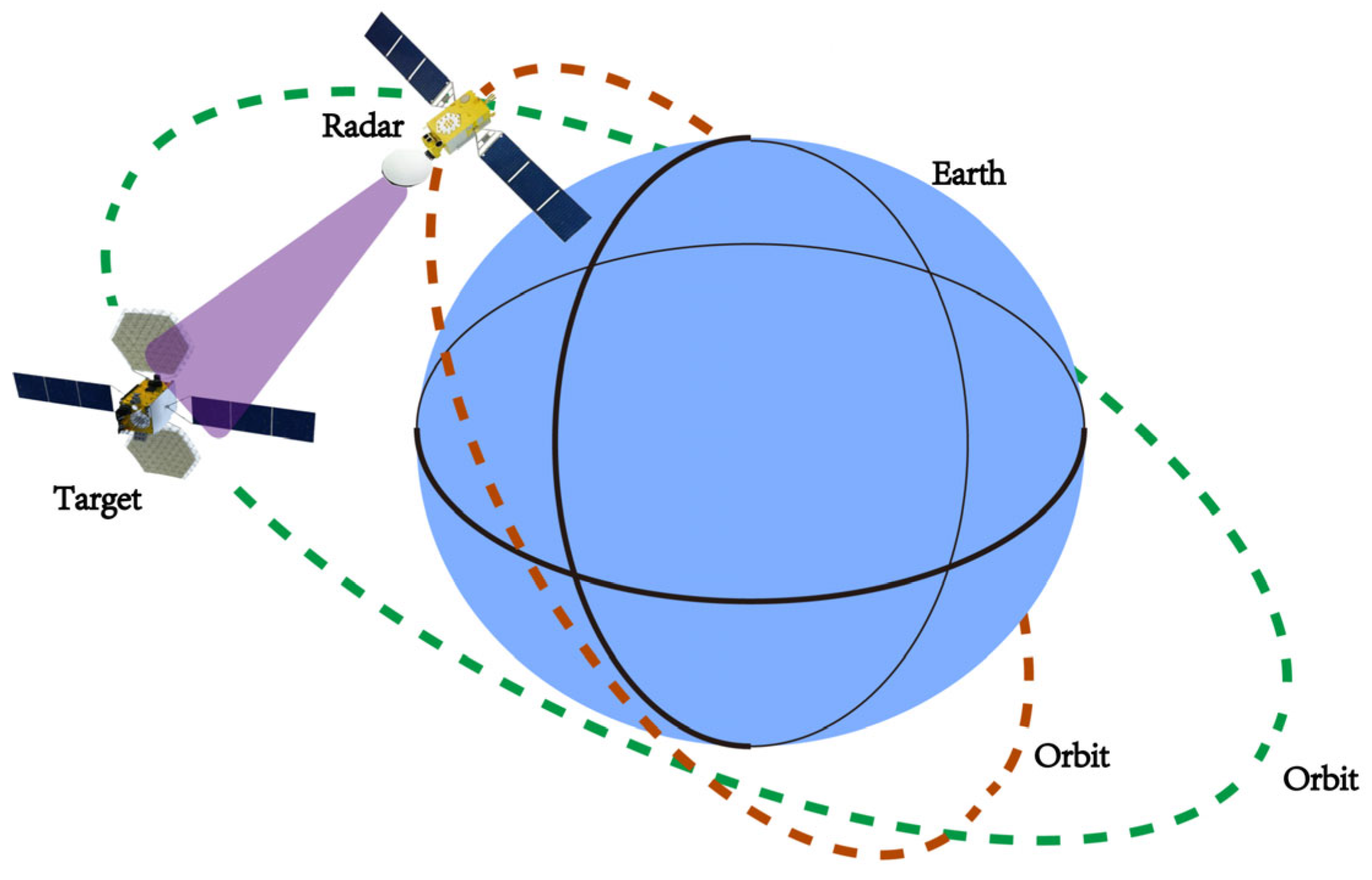
2.1. Spaceborne THz-ISAR Signal Model and Boundary Condition Analysis

A schematic diagram of the spaceborne terahertz radar imaging scenario is shown in Figure 1.

Assume that the radar emits an LFM signal:

$$s\left(\widehat{t},t_m\right)=A\cdot \mathrm{rect}\left[{\displaystyle \frac{t}{T_p}}\right]\cdot \exp \left(j2\pi f_{c}t+j\pi \gamma {\widehat{t}}^2\right)$$

(1)

The corresponding echo signal can be expressed as:

$$s_r\left(\widehat{t},t_m\right)=\sigma A\cdot \mathrm{rect}({\displaystyle \frac{t-2R(\widehat{t},t_m)/c}{T_p}})\exp \left(j2\pi f_c(t-2R(\widehat{t},t_m)/c)+j\pi \gamma {(\widehat{t}-2R(\widehat{t},t_m)/c)}^2\right)$$

(2)

In Equations (1) and (2), $\sigma$ is the attenuation coefficient of the echo, A is the magnitude of the echo signal, $T_p$ is the pulse-width of the signal, $\gamma$ is the chirp rate of the signal, $c$ is the speed of light, $f_c$ denotes the frequency of the signal, $\widehat{t}$ and $t_m$ denotes fast-time and slow-time respectively. $R\left(\widehat{t},t_m\right)$ denotes the radial distance between the target and the radar. Due to the high-speed translation of the target, the traditional stop-and-go model is no longer applicable. Consequently, $R\left(\widehat{t},t_m\right)$ becomes a variable dependent on both slow-time (inter-pulse) and fast-time (intra-pulse). For analytical clarity, the radial distance $R\left(\widehat{t},t_m\right)$ can be decomposed into two components dependent on fast-time and slow-time, respectively:

$$R(\widehat{t},t_m)=R(t_m)+v_m\widehat{t}$$

(3)

where $R\left(t_m\right)$ represents the inter-pulse range walk. $v_m$ denotes the translational velocity at the moment of $t_m$, $v_m\widehat{t}$ refers to the intra-pulse range walk. The signal after Dechirp can be written as:

$$\begin{array}{ll}{s}_d\left(\widehat{t},t_m\right)=& \sigma A\cdot \mathrm{rect}\left({\displaystyle \frac{(1-2v_m/c)\widehat{t}-2R(t_m)/c}{T_p}}\right)\\ & \cdot \exp \left(-j{\displaystyle \frac{4\pi }{\lambda }}\left(R(t_m)-R_{ref}\right)\right)\cdot \exp \left(j4\pi {\displaystyle \frac{\gamma }{c^2}}\left(R^2(t_m)-R_{ref}^2\right)\right)\\ & \cdot \exp \left(-j4\pi \left({\displaystyle \frac{\gamma }{c}}\left(R(t_m)-R_{ref}\right)+{\displaystyle \frac{v_m}{\lambda }}-2\gamma v_m{\displaystyle \frac{R(t_m)}{c^2}}\right)\widehat{t}\right)\\ & \cdot \exp \left(j4\pi {\displaystyle \frac{v_m}{c}}\gamma \left({\displaystyle \frac{v_m}{c}}-1\right){\widehat{t}}^2\right)\end{array}$$

(4)

where $R_{ref}$ stands for the reference distance in the Dechirp process. For simplicity, the envelope term $\mathrm{rect}\left(\cdot \right)$ will temporarily not be considered in the following derivation. Set:

$$\left\{\begin{array}{l}{f}_m=2{\displaystyle \frac{\gamma }{c}}\left(R(t_m)-R_{ref}\right)+2{\displaystyle \frac{v_m}{\lambda }}-4\gamma v_m{\displaystyle \frac{R(t_m)}{c^2}}\\ {\beta }_m=2{\displaystyle \frac{v_m}{c}}\gamma \left({\displaystyle \frac{v_m}{c}}-1\right)\end{array}\right.$$

(5)

Then, Equation (4) can be re-written as:

$$\begin{array}{ll}{s}_d\left(\widehat{t},t_m\right)=& \sigma A\cdot \exp \left(-j{\displaystyle \frac{4\pi }{\lambda }}\left(R(t_m)-R_{ref}\right)\right)\\ & \cdot \exp \left(j4\pi {\displaystyle \frac{\gamma }{c^2}}\left(R^2(t_m)-R_{ref}^2\right)\right)\\ & \cdot \exp \left(-j2\pi f_m\widehat{t}\right)\\ & \cdot \exp \left(j2\pi {\beta }_m{\widehat{t}}^2\right)\end{array}$$

(6)

Since the third exponential term contains only a linear phase component associated with the fast-time $\widehat{t}$, it will only affect the range migration of the envelope, which has no impact on image quality. Therefore, we first isolate the analysis of the fourth exponential term, which contains a quadratic component with respect to the fast time $\widehat{t}$. Performing the Fourier transform on this term yields:

$$\begin{array}{ll}U\left(f,t_m\right)& ={\displaystyle {\int }_{-T_p/2}^{T_p/2}\exp \left(j2\pi {\beta }_m{\widehat{t}}^2\right)}\cdot \exp \left(-j2\pi f \widehat{t}\right)d\widehat{t}\\ & \approx \exp \left(-j\left({\displaystyle \frac{\pi f^2}{2{\beta }_m}}+{\displaystyle \frac{\pi }{4}}\right)\right)\end{array}$$

(7)

To ensure the coherence of the main text, the detailed derivation of the above formulas is provided in Appendix A. According to Equation (7), the second-order phase error induced by the target’s high-speed motion is denoted as:

$$\mathrm{SOE}=\left|{\displaystyle \frac{\pi f^2}{2{\beta }_m}}+{\displaystyle \frac{\pi }{4}}\right|$$

(8)

where $\left|\cdot \right|$ denotes taking the absolute value. Only when $\mathrm{SOE}<{\displaystyle \frac{\pi }{4}}$ the effect of it can be ignored. Since the maximum value of $\mathrm{SOE}$ can be achieved when $f=\pm B/2$, where $B$ refers to the bandwidth of the radar signal, the boundary condition can be written as:

$$\left|{\displaystyle \frac{\pi B^2}{8{\beta }_m}}\right|<{\displaystyle \frac{\pi }{4}}\Rightarrow \left|{\beta }_m\right|>{\displaystyle \frac{B^2}{2}}\Rightarrow {\displaystyle \frac{v_m}{c}}\gamma \left(1-{\displaystyle \frac{v_m}{c}}\right)>{\displaystyle \frac{B^2}{4}}$$

(9)

Since $\gamma ={\displaystyle \frac{B}{T_p}}$, the boundary condition in 9 can be further written as:

$${\displaystyle \frac{v_m}{c}}\left(1-{\displaystyle \frac{v_m}{c}}\right)>{\displaystyle \frac{B{T}_p}{4}}$$

(10)

However, in THz-ISAR imaging, the time–bandwidth product (TBP) of radar signals is typically extremely large, making it challenging to satisfy the boundary conditions in Equation (10). Based upon the signal model and the boundary condition analyzed before, despite the high speed of targets, bandwidth of THz radar and the signal pulse width collectively affects the outcomes of range compression, we mainly focus on the high speed of targets and the large bandwidth brought by THz radar in this study. There are two main reasons for this consideration: firstly, as evidenced by the boundary condition, signal bandwidth and pulse width occupy symmetric positions in the mathematical expression. Consequently, variations in these two parameters should impose analogous effects on the one-dimensional range profiles, which is going to be verified by the simulation experiments in Section 3. Secondly, when constructing the joint compensation term in the following section, the existence of pulse width has already been incorporated.

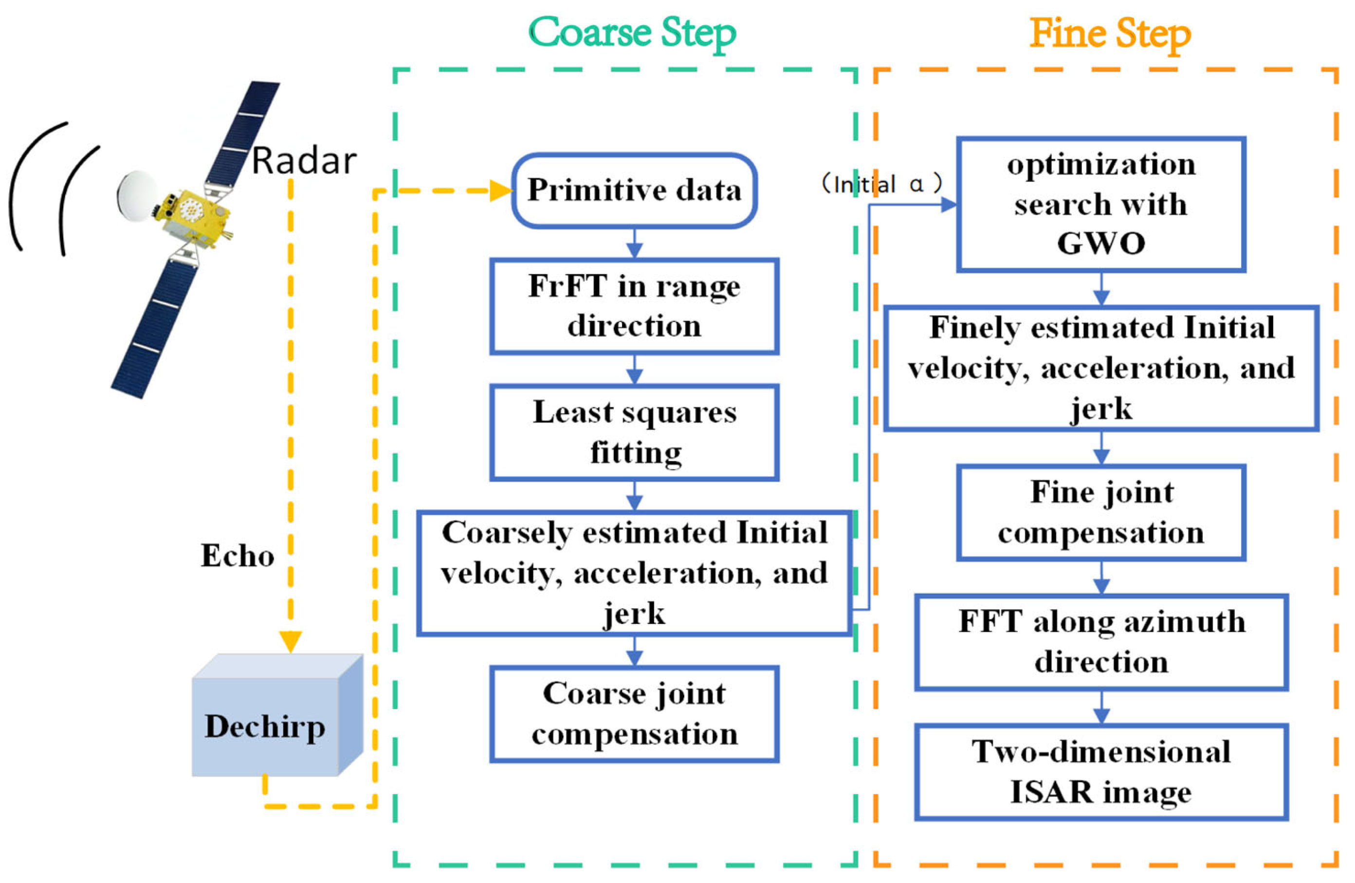
2.2. Spaceborne THz-ISAR Imaging Process and Algorithm

By comparing with the echo signal under a stop-and-go model, it can be concluded that the additional exponential terms in the echoes obtained under high-speed scenarios compared to those derived from the stop-and-go model are:

$$\left\{\begin{array}{l}\exp \left(-j4\pi {\displaystyle \frac{v_m}{\lambda }}\widehat{t}\right)\\ \exp \left(j4\pi {\displaystyle \frac{v_m}{c}}\gamma \left({\displaystyle \frac{v_m}{c}}-1\right){\widehat{t}}^2\right)\end{array}\right.$$

(11)

Based on the foregoing derivations, the intra-pulse compensation term can be defined as:

$$C_{\mathrm{intra}}=\exp \left(j4\pi {\displaystyle \frac{v_m}{\lambda }}\widehat{t}\right)\cdot \exp \left(-j4\pi {\displaystyle \frac{v_m}{c}}\gamma \left({\displaystyle \frac{v_m}{c}}-1\right){\widehat{t}}^2\right)$$

(12)

Assuming that intra-pulse compensation has been completed and setting ${\alpha }_m=1-2{\displaystyle \frac{v_m}{c}}$, performing the Fourier transform along the fast-time $\widehat{t}$. After RVP compensation and neglecting the residual phase, the signal model can be rewritten as:

$$\begin{array}{ll}{S}_{\mathrm{afterintra}}\left(f,t_m\right)=& \sigma A\cdot {\displaystyle \frac{T_p}{{\alpha }_m}}\sin c\left({\displaystyle \frac{T_p}{{\alpha }_m}}\left(f+2{\displaystyle \frac{\gamma }{c}}\left({\alpha }_{m}R(t_m)-R_{ref}\right)\right)\right)\\ & \cdot \exp \left(-j{\displaystyle \frac{4\pi }{\lambda }}\left(R(t_m)-R_{ref}\right)\right)\end{array}$$

(13)

In the ISAR imaging process, the motion of a target relative to the radar can be decomposed into translational and rotational components. Given the radar–target distance of hundreds of kilometers in spaceborne THz-ISAR imaging scenario, the planar wave assumption holds. Let $R_r\left(t_m\right)$ represent the translational motion component and $R_a\left(t_m\right)$ denote the rotational motion component, then we have:

$$R(t_m)=R_r(t_m)+R_a(t_m)$$

(14)

Substituting Equation (14) into Equation (13) yields:

$$\begin{array}{ll}{S}_{\mathrm{afterintra}}\left(f,t_m\right)=& \sigma A\cdot {\displaystyle \frac{T_p}{{\alpha }_m}}\sin c\left({\displaystyle \frac{T_p}{{\alpha }_m}}\left(f+2{\displaystyle \frac{\gamma }{c}}\left({\alpha }_m\left(R_r(t_m)+R_a(t_m)\right)-R_{ref}\right)\right)\right)\\ & \cdot \exp \left(-j{\displaystyle \frac{4\pi }{\lambda }}\left(R_r(t_m)+R_a(t_m)-R_{ref}\right)\right)\end{array}$$

(15)

Based on the properties of the Fourier transform, shifting the $\sin c$ function in the frequency domain requires multiplying the corresponding term in the time domain. Meanwhile, phase errors caused by translational motion can be eliminated by directly multiplying the corresponding compensation term in the time domain. Therefore, the inter-pulse compensation term should be:

$$C_{\mathrm{inter}}=\exp \left(-j4\pi {\displaystyle \frac{T_p\gamma }{{\alpha }_{m}c}}{R}_r\left(t_m\right)\widehat{t}\right)\cdot \exp \left(j4\pi {\displaystyle \frac{R_r\left(t_m\right)}{\lambda }}\right)$$

(16)

The joint motion compensation term can be derived as:

$$\begin{array}{ll}{C}_{\mathrm{joint}}=& \exp \left(-j4\pi {\displaystyle \frac{T_p\gamma }{{\alpha }_{m}c}}{R}_r\left(t_m\right)\widehat{t}\right)\cdot \exp \left(j4\pi {\displaystyle \frac{R_r\left(t_m\right)}{\lambda }}\right)\\ & \cdot \exp \left(j4\pi {\displaystyle \frac{v_m}{\lambda }}\widehat{t}\right)\cdot \exp \left(-j4\pi {\displaystyle \frac{v_m}{c}}\gamma \left({\displaystyle \frac{v_m}{c}}-1\right){\widehat{t}}^2\right)\end{array}$$

(17)

Based on the foregoing derivations, it can be observed that the key to joint compensation lies in the accurate estimation of the target’s translational parameter $v_m$ and its motion trajectory $R_r\left(t_m\right)$. In practical space target motion scenarios, since the radar pulse duration is extremely short, the target’s velocity within a single echo can be approximated as uniform. However, during the entire coherent integration time for imaging, the radial velocity $v_m$ of the space target exhibits variations. Without loss of generality, the radial velocity can be modeled as a second-order polynomial function of slow time:

$$v_m=v_0+a\cdot t_m+a^{\prime }\cdot t_m^2$$

(18)

where $v_0$ represents the initial velocity of the target translation, while $a$ and $a^{\prime }$ denote the target acceleration and jerk, respectively. Based on Equation (18), the translational displacement of the target relative to the initial time at slow time $t_m$ can be expressed as:

$$R_r(t_m)=v_0{t}_m+{\displaystyle \frac{1}{2}}a\cdot t_m^2+{\displaystyle \frac{1}{3}}{a}^{\prime }\cdot t_m^3$$

(19)

Therefore, the joint compensation function can be expressed as ${\mathbf{C}}_{\mathrm{joint}}(\overrightarrow{\mathit{l}})$,where:

$$\overrightarrow{\mathit{l}}=\left\{v_0,a,a^{\prime }\right\}$$

(20)

To achieve precise estimation of target motion parameters and accurate joint compensation, this paper proposes a novel algorithm combining FrFT-based coarse joint compensation and Grey Wolf Optimizer (GWO)-based fine joint compensation. The specific steps are as follows:

• FrFT is used to coarsely estimate the chirp rate of each pulse;
• Convert the chirp rate obtained in step 1 into velocity, fit the motion parameters using the least squares method, and perform coarse joint compensation;
• Calculate the synthetic waveform entropy (SWE) of the one-dimensional range profile after the coarse joint compensation in step 2.
• Use the SWE of the one-dimensional range profile as the cost function, with its initial value derived from the result in step 3, and the coarsely estimated parameters obtained in step 2 as the $\alpha$ wolf in the GWO algorithm, iteratively search for the optimal motion parameter estimates that minimize the SWE.
• Use the estimated parameters in step 4 to perform the precise joint compensation for the echo, and perform Fourier transform along the azimuth direction. A well-focused ISAR image is finally acquired.

The processing flowchart is shown in Figure 2. The following sections provide detailed descriptions of each step.

2.2.1. FrFT-Based Coarse Joint Compensation Method

Previous analyses have demonstrated that the demodulated echo signals of high-speed targets exhibit typical LFM characteristics in the fast-time dimension. This observation provides a theoretical foundation for employing the FrFT to accomplish parameters estimation and motion compensation. FrFT is a global linear time–frequency analysis tool that inherently matches the characteristics of LFM signals. Applying the FrFT to the receiving signal yields:

$${\mathcal{F}}^p\left\{s_d\left(\widehat{t},t_m\right)\right\}\left(u\right)={\displaystyle {\int }_{-\infty }^{\infty }{s}_d\left(\widehat{t},t_m\right)\cdot K_p\left(\widehat{t},u\right)}d\widehat{t}$$

(21)

where ${\mathcal{F}}^p$ is the FrFT Operator, $\varphi$ is a constant independent of $\widehat{t}$, $p$ is the rotation angle, and $K_p\left(\widehat{t},u\right)$ is the FrFT Kernel. When the rotation angle $p$ meets $p=-\mathrm{arccot}2{\beta }_m$, Equation (21) can be derived as:

$$\begin{array}{ll}{\mathcal{F}}^p\left\{s_d\left(\widehat{t},t_m\right)\right\}\left(u\right)=& \sigma A\cdot \sqrt{{\displaystyle \frac{1+j2{\beta }_m}{2\pi }}}\cdot {\displaystyle \frac{1}{\sqrt{4{\beta }_m^2+1}}}\cdot \delta \left(u+{\displaystyle \frac{f_m}{\sqrt{4{\beta }_m^2+1}}}\right)\\ & \cdot \exp \left(-j2\pi {\beta }_m{u}^2\right)\cdot \exp \left(j\varphi \right)\end{array}$$

(22)

Detailed derivation process of Equation (22) is provided in Appendix B. Equation (22) indicates that when an appropriate rotation angle is selected for the FrFT, the influence of the frequency modulation term is eliminated, allowing for a well-focused one-dimensional range profile. It is important to note that in the discretization process, the relationship between the rotation angle and the chirp rate is given by:

$$2{\beta }_m=-{\displaystyle \frac{f_s}{T_p}}\cot p$$

(23)

where ${\displaystyle \frac{f_s}{T_p}}$ serves as the normalization factor. Then, the discrete velocity–time sequence denoted as ${\left\{\left(v_m,t_m\right)\right\}}_{m=1}^M$ is obtained, while $M$ denotes the number of pulses accumulated during the coherent integration time.

Since the computational complexity of searching for the optimal rotation angle in the FrFT necessitates subsampling, we select parts of pulses to generate the velocity–time sequence, followed by least squares fitting to obtain a coarse estimation of target parameters. This approach achieves a critical balance between coarse compensation accuracy and computational efficiency. The exemplary steps are as follows:

• For $m=1:{\displaystyle \frac{M}{2}}$ (Let $M$ be an even integer), use FrFT to obtain $v_m$;
• To eliminate abrupt error, set empirical value $\zeta$, if $|v_m-v_{m-1}|>\zeta$ or $|v_m-v_{m+1}|>\zeta$ ($1<m<{\displaystyle \frac{M}{2}}$), then set $v_m=(v_{m-1}+v_{m+1})/2$;
• For the discrete velocity–time observation sequence ${\left\{\left(v_m,t_m\right)\right\}}_{m=1}^{M/2}$, assuming its adherence to a model: ${\widehat{v}}_m=v_0+a{t}_m+a^{\prime }{t}_m^2$, formulate the parameter estimation problem as a least squares optimization: $\underset{v_0,a,a^{\prime }}{\min }{{\displaystyle \sum _{m=1}^{M/2}\left(v_m-{\widehat{v}}_m\right)}}^2$ to obtain the estimated parameters;

Then, the coarsely estimated parameters obtained in the above process can be used to achieve coarse joint compensation. Based on the preceding analysis, the coarse joint compensation function $C_{\mathrm{joint}}({\overrightarrow{l}}_{\mathrm{coarse}})$ can be derived from the fitted velocity–time relationship. Utilizing this function $C_{\mathrm{joint}}({\overrightarrow{l}}_{\mathrm{coarse}})$, coarse joint compensation for high-speed moving targets is achieved. Simultaneously, the fitted initial velocity, acceleration, and jerk of the target are recorded as the alpha individuals in the subsequent refined compensation using the GWO algorithm.

2.2.2. GWO-Based Fine Joint Compensation Method

In the Grey Wolf Optimizer (GWO), to mathematically simulate the social hierarchy of wolves, the optimal solution is defined as $\alpha$, representing the position of the leading wolf. The suboptimal and third-best solutions are named $\beta$ and $\epsilon$, respectively, mimicking the positions of second- and third-tier wolves. The remaining candidate solutions are designated as $\omega$ wolves, symbolizing the positions of subordinate wolves. In the GWO algorithm, the hunting process (solution search process) is guided by the $\alpha$, $\beta$, and $\epsilon$ wolves, while the $\omega$ wolves update their positions by following these three leaders.

The optimal solution searching steps of GWO are as follows:

• A population of grey wolf individuals is randomly initialized, where each individual’s position represents a candidate solution to the optimization. Define a convergence parameter $a$ to control the searching scope;
• Calculate each grey wolf’s fitness value to determine $\alpha$, $\beta$, and $\epsilon$. In this paper, $\alpha$ is the coarse estimation result of Section 2.2.1;
• $\epsilon$ adjusts its movement direction based on the positions of the three leaders, whose positions indicate the current most promising regions;
• The $\alpha$, $\beta$, and $\epsilon$ wolves assess their distance to the optimal solution and adaptively adjust their positions. $\epsilon$ adjusts its positions based on the positions of the three leaders. Re-evaluate the fitness of each grey wolf and update the leaders;
• The algorithm terminates when either the maximum iteration threshold is reached or the obtained solution is good enough and the position of $\alpha$ serves as the optimal solution. Otherwise, repeat step 3 and 4.

We now examine the fitness function implemented within GWO algorithm. In previous sections, the analyses of the compensation method are only based on a single scatter and a single pulse. However, there should be a bunch of scatters and hundreds of pulses in practical scenario; therefore, the echo data should be expressed as $I\left(n,m\right)$, where $I\left(n,m\right)$ refers to a data matrix, $n$ and $m$ denote the particular sampling point and pulse in the data matrix, respectively. Assuming there are $P$ scatters, the data matrix after joint motion compensation can be expressed as:

$$\begin{array}{ll}I\left(n,m\right)=& {\displaystyle \sum _{i=1}^P{\displaystyle \sum _{n=1}^{N_r}{\displaystyle \sum _{m=1}^{N_a}{\sigma }_i{A}_i}}}\\ & \cdot \sin c\left({\displaystyle \frac{T_p}{{\alpha }_m}}\left({\displaystyle \frac{n}{N_r}}{f}_s+2{\displaystyle \frac{\gamma }{c}}\left({\alpha }_m{\psi }_m+R_a\left(t_m\right)\right)-R_{ref}\right)\right)\\ & \cdot \exp \left(-j4\pi {\displaystyle \frac{{\psi }_m}{\lambda }}\right)\cdot \exp \left(-j4\pi {\displaystyle \frac{R_a\left(t_m\right)-R_{ref}}{\lambda }}\right)\end{array}$$

(24)

where $N_r$ denotes the sampling points and $N_a$ denotes the number of pulses during the imaging period. Let $r_m$ be the translational migration calculated by the estimated motion parameters (initial velocity $v_{0est}$, acceleration $a_{est}$ and jerk $a_{est}^{\prime }$), then:

$$\left\{\begin{array}{l}{\psi }_m=R_r\left(t_m\right)-r_m\\ r_m=v_{0est}{t}_m+{\displaystyle \frac{1}{2}}{a}_{est}{t}_m^2+{\displaystyle \frac{1}{3}}{a}_{est}^{\prime }{t}_m^3\\ t_m={\displaystyle \frac{m}{PRF}}\end{array}\right.$$

(25)

Based on the foregoing derivations, $\mathrm{abs}\left(I\left(n,m\right)\right)$ represents the one-dimensional range profile after joint motion compensation, $\mathrm{abs}\left(\cdot \right)$ indicates taking the absolute value. Since the one-dimensional range profile after joint motion compensation is intricately linked with the joint motion compensation term, it can be further written as $\mathrm{abs}\left(I\left(n,m\right);C\left(\overrightarrow{l}\right)\right)$. Drawing on the concept of waveform entropy, the entropy of the synthesized waveform is calculated by combining the range profiles from multiple pulses. Obviously, if the intra-pulse compensation effectively corrects the main lobe broadening (sharpening the peak) and the inter-pulse compensation achieves precise envelope alignment, the peaks from different pulses will coherently superimpose, resulting in a more sharped synthesized waveform with lower entropy. Conversely, poor intra-pulse and inter-pulse compensation will cause misalignment of peaks, leading to a flattened envelope of the synthesized waveform and higher entropy. Let the synthesized waveform be denoted as ${\mathbf{Env}}_{\mathbf{t}}$, which is an $N_r\times 1$ vector. For any distance sampling point $n$, the following relationship holds:

$${\mathbf{Env}}_{\mathbf{t}}\left(n;C\left(\overrightarrow{l}\right)\right)={\displaystyle \sum _{m=1}^{N_a}\mathrm{abs}\left(I\left(n,m\right);C\left(\overrightarrow{l}\right)\right)}$$

(26)

Assume the synthesized range vector is ${\mathbf{Env}}_{\mathbf{t}}={\left[e_1 e_2 \cdots e_{N_r}\right]}^T$. The values of this range vector are normalized to obtain ${\mathbf{Env}}_{\mathbf{0}}$, where each normalized element satisfies $e_i^0=e_i/{\displaystyle \sum _{i=1}^{N_r}{e}_i}\left(i=1,\cdots ,N_r\right)$, and ${\displaystyle \sum _{i=1}^N{e}_i^0=1}$. Since the normalized values exhibit probability-like properties, the waveform entropy can be formulated as:

$$\mathbf{H}\left(C\left(\overrightarrow{l}\right)\right)=-{\displaystyle \sum _{n=1}^{N_r}{\mathbf{Env}}_0}\left(n;C\left(\overrightarrow{l}\right)\right)\ln {\mathbf{Env}}_{\mathbf{0}}\left(n;C\left(\overrightarrow{l}\right)\right)$$

(27)

Therefore, the GWO algorithm’s task is to find the optimal $\overrightarrow{l}$, which helps to obtain minimum $\mathbf{H}\left(C\left(\overrightarrow{l}\right)\right)$.

3. Results

In this section, we firstly use simulation experiments to showcase the negative effect on imaging brought by high-speed of the target, large bandwidth of THz-radar as well as the pulse width. Then, a simulation experiment verifying the FrFT-based parameter estimation method is conducted. Then, point cloud scattering model simulation data, the complex scattering model electromagnetic calculation data, and the field-measured data are used to verify the effectiveness of the proposed spaceborne THz-ISAR imaging algorithm and processing flow.

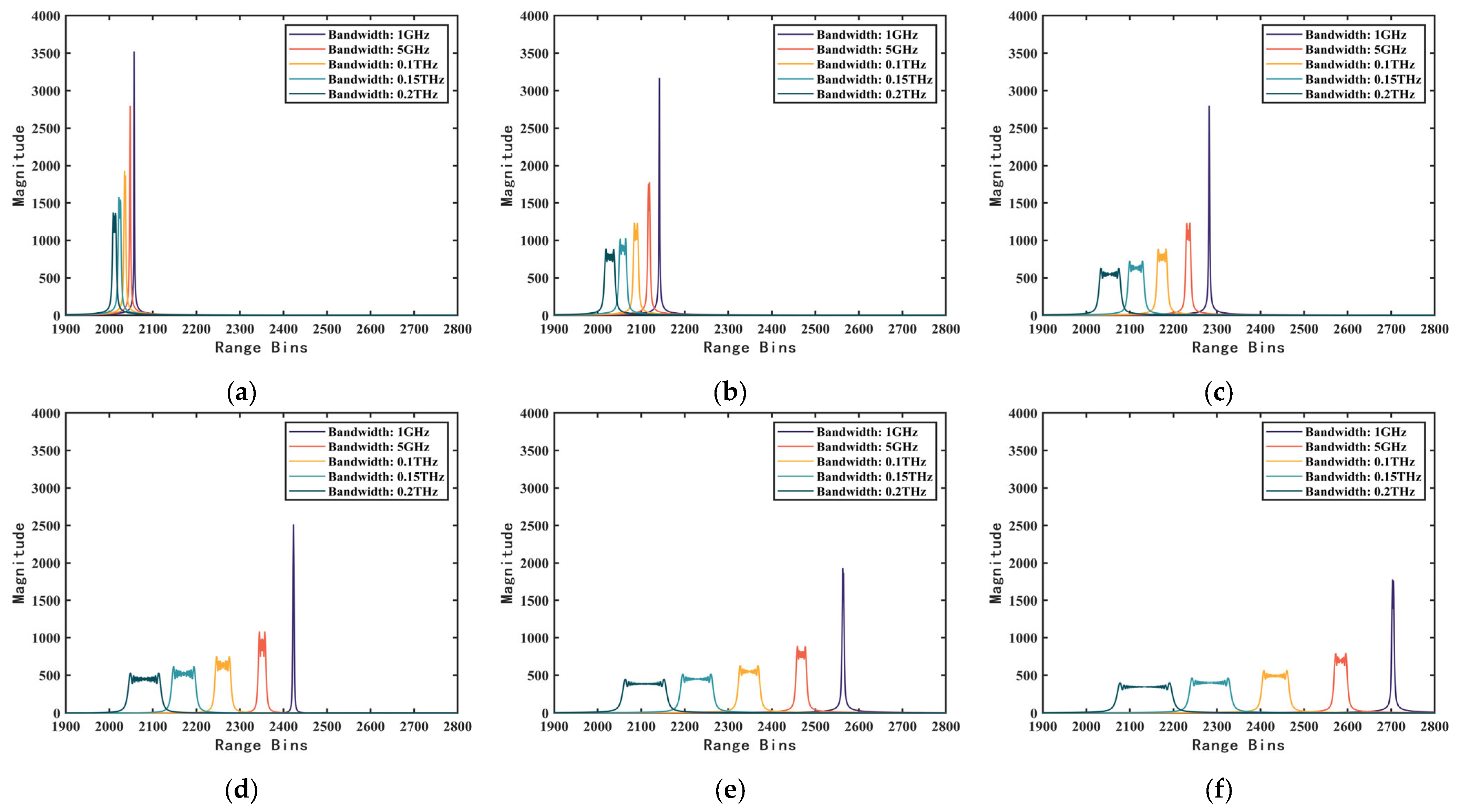
3.1. Simulation Experiments on the Co-Effect of Paramters Based on Single Scattering Point

Based on a single scattering point, we conducted a simulation experiment; the compression results of range profiles are shown below. Figure 3 shows the effect of different target velocities and pulse widths in THz-ISAR imaging since we have fixed the signal bandwidth at 10 GHz, while Figure 4 shows the effect of different target velocities and bandwidths due to the fixation of pulse width of 200 μs. It can be seen from the results that as the target velocity increases and the bandwidth expands, the mainlobe broadening after range compression becomes more severe, accompanied by a frequency–domain shift.

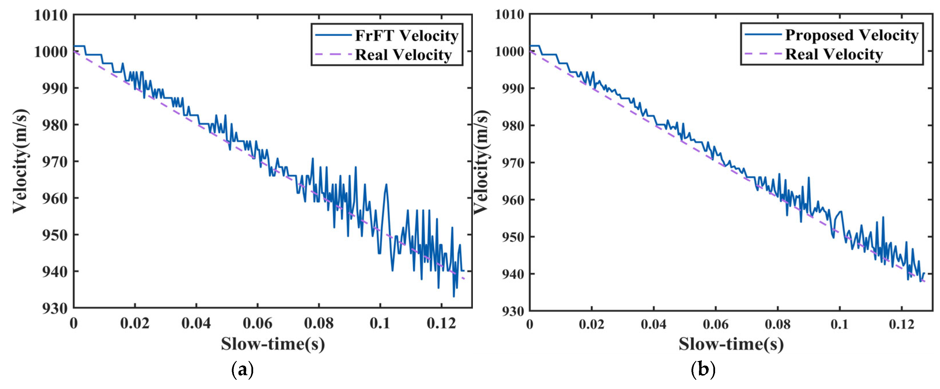
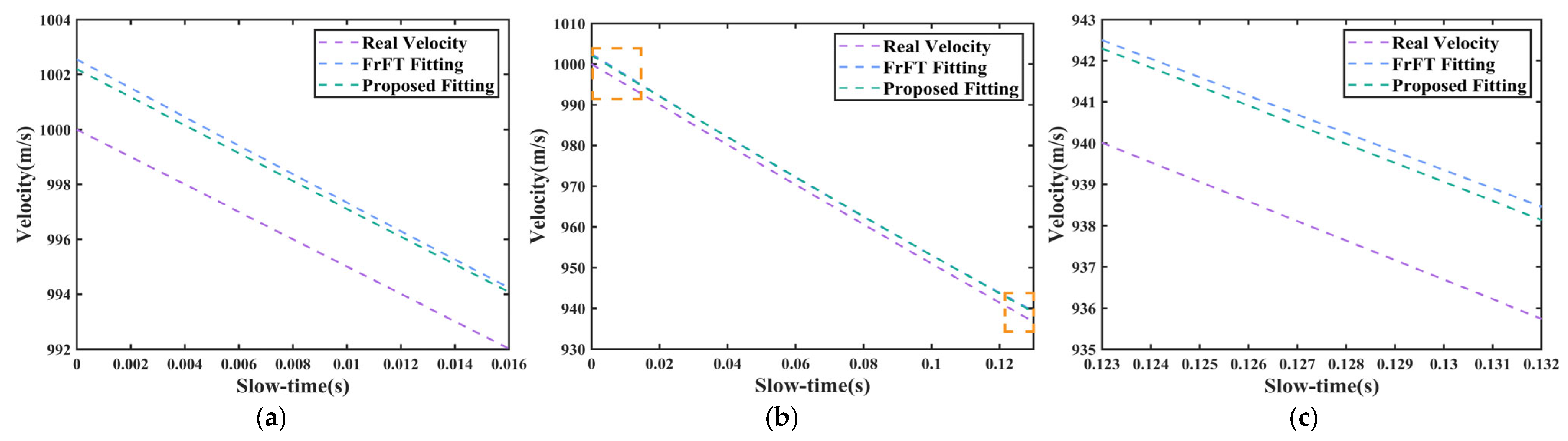
3.2. Simulation Experiment Verifying the FrFT-Based Parameter Estimation Method

Table 1. Simulation configuration for velocity estimation.

Parameters	Value	Target Parameters	Value
Carrier frequency	220 GHz	Initial velocity	1000 m/s
Pulse width	50 μs	Acceleration	−500 m/s2
Bandwidth	10 GHz	Jerk	100 m/s3
PRF	5000 Hz	Slant range	300 km

systematically delineates the simulation parameters configuration, with the left column specifying THz radar operational parameters and the right column detailing target dynamics. The radar system operates at 220 GHz carrier frequency with 10 GHz bandwidth and 50 μs pulse duration—canonical parameters for modern terahertz radar systems. The target exhibits sophisticated motion characteristics: initial velocity of 1000 m/s, acceleration of −500 m/s², jerk of 100 m/s³, and reference range of 300 km. During the simulation with a coherent processing interval containing 512 pulses, we selected the initial 256 pulses for illustration.

Figure 5 and Figure 6 demonstrate the efficacy of our method in motion parameter estimation under simulated scenarios.

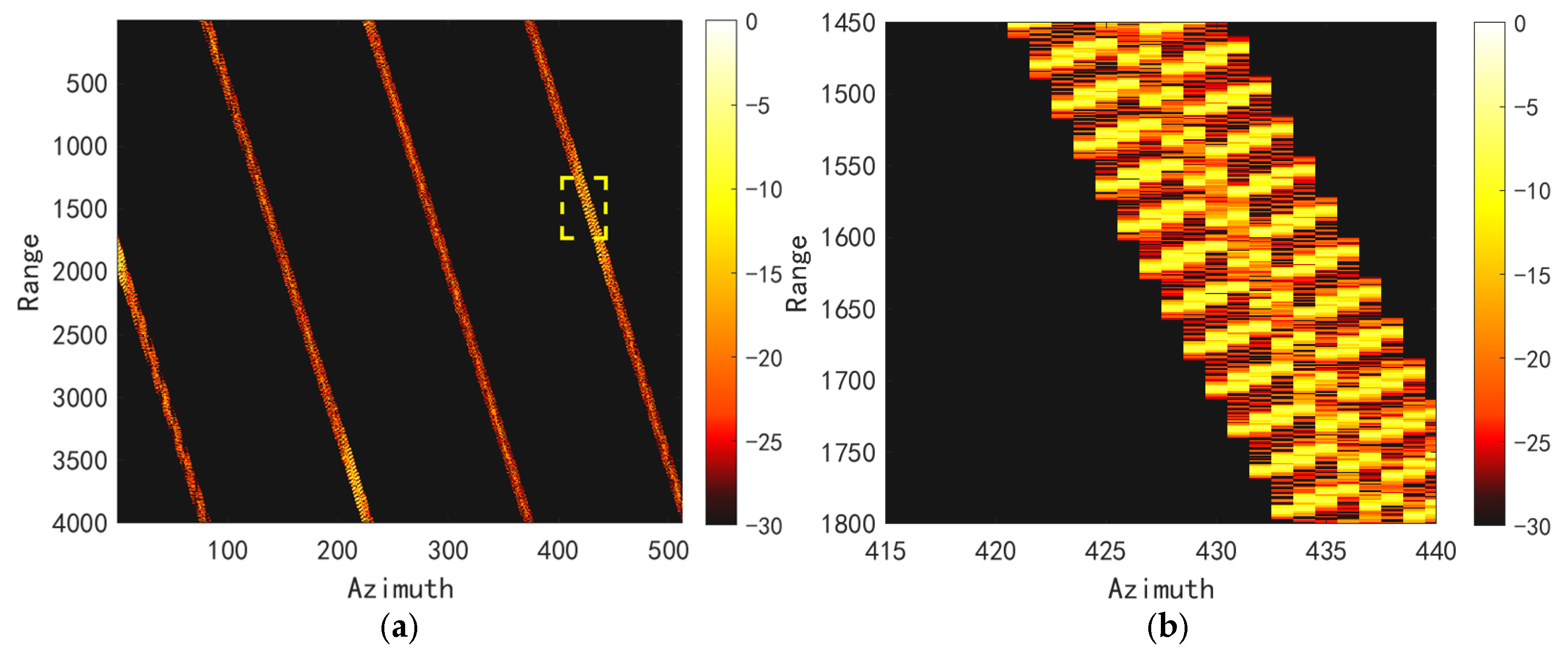
3.3. Satellite Point Cloud Model Simulation Experiments

In this section, 544 points of simulation data as shown in Figure 7 are used for experiments.

The echo is generated by the signal model in Section 2.

Table 2. Simulation configuration for point cloud model experiments.

Parameters	Value	Target Parameters	Value
Carrier frequency	220 GHz	Initial velocity	1000 m/s
Pulse width	50 μs	Acceleration	−500 m/s2
Bandwidth	0.1 THz	Jerk	100 m/s3
PRF	5000 Hz	Slant range	300 km
Light velocity	3 × 108 m/s	Rotation velocity	0.5 rad/s

shows the simulation configuration, which is approximately the same as the configurations in Table 1.

In this experiment, 512 echo data samples are processed. The following figures show the range profile before intra-pulse compensation and the range profile after intra-pulse compensation, the range profile after coarse inter-pulse compensation and the range profile after fine inter-pulse compensation. In the end, two ISAR images, whose differences with another lies in whether intra-pulse compensation has been applied during signal processing, are compared.

A comparative analysis of Figure 8 and Figure 9 reveals significant main lobe broadening and defocusing in the range profile compression results prior to intra-pulse compensation. Following the implementation of intra-pulse compensation, the main lobe broadening is effectively mitigated, achieving superior compression and focusing performance. Additionally, the comparison between Figure 8b and Figure 9b demonstrates a frequency shift induced by the first-order phase term, which, however, does not adversely affect the overall image quality. To explicitly demonstrate the impact of range profile main lobe broadening on ISAR imaging quality, we perform conventional envelope alignment on the one-dimensional range profiles before and after intra-pulse compensation, followed by azimuth Fourier transform to generate the ISAR images as shown in Figure 10.

Results in Figure 10 demonstrate that prior to intra-pulse compensation, the main lobe broadening in the one-dimensional range profile caused by target’s high-speed motion significantly degrades the performance of conventional adjacent correlation-based envelope alignment. This degradation prevents the azimuth Fourier transform of the uncompensated range profile (in Figure 10b) from generating a well-focused 2D ISAR image. In contrast, after implementing intra-pulse compensation, the main lobe broadening is effectively suppressed. The conventional envelope alignment method successfully achieves coherent registration of successive echoes, enabling the azimuth Fourier transform of the compensated range profile (in Figure 10e) to produce a sharply focused 2D ISAR image.

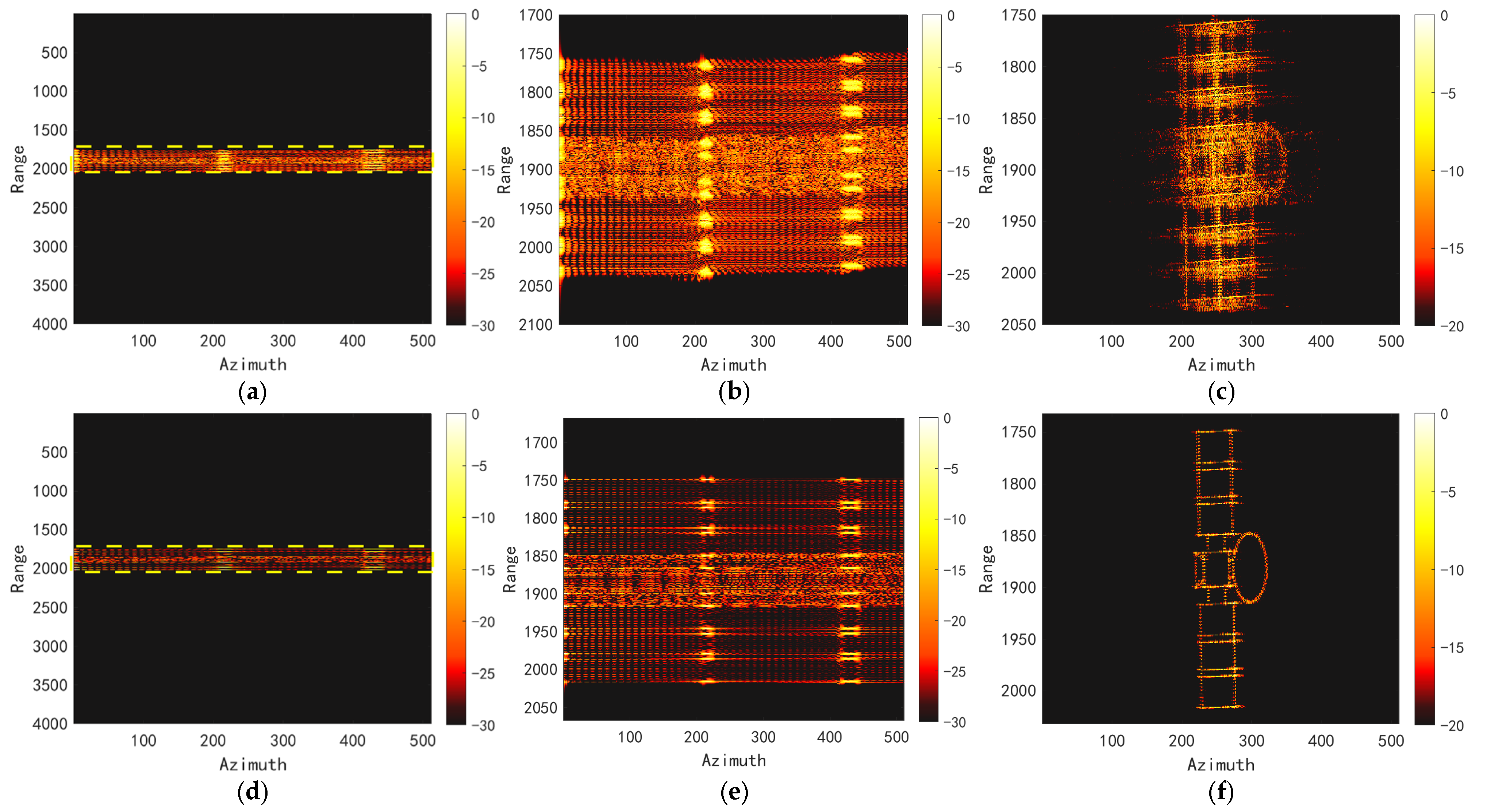
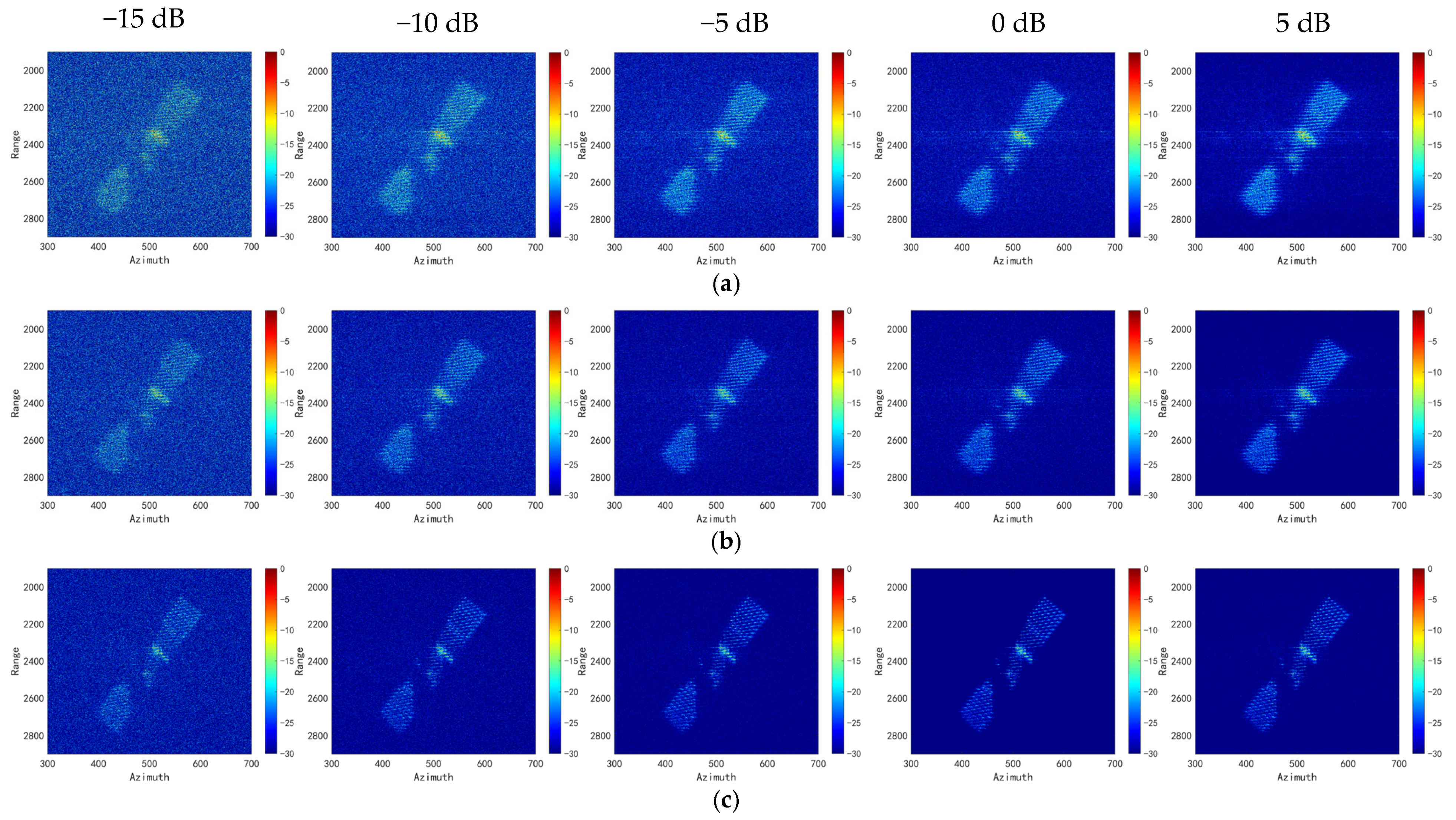
3.4. Satellite Electromagnetic Simulation Experiments

In this section, we use the satellite model (Figure 11) electromagnetic simulation data to further verify the superiority of our method. The primitive electromagnetic simulation data is obtained through a turntable model, which means the high-speed translation has to be added into the data, so that further analysis can be carried out. We use the following translation parameters: the initial velocity 2000 m/s, the acceleration −500 m/s² and the jerk 10 m/s³. The radar parameters are set as follows: the carrier frequency is 216 GHz, the signal bandwidth is 0.2 THz, the PRF is 625 Hz, and the pulse duration is 36 us. A total of 625 pulses during the observation time are analyzed.

Two conventional motion compensation methods for high-speed targets are currently employed: FrFT-based individual compensation, which independently searches for the optimal rotation angle for each pulse and corrects phase errors, and Particle Swarm Optimization (PSO)-based global search. To rigorously validate the superiority of our proposed method, we adhere to the controlled variable methodology by comparing it against a hybrid benchmark combining FrFT-based coarse compensation and PSO-based fine compensation.

Three methods mentioned above are used for intra- and inter-pulse compensation of high-speed target echoes, and their corresponding one-dimensional range profiles are comparatively illustrated in Figure 12. It is critical to highlight that during the fine compensation phase, both the PSO and GWO algorithms were configured with identical parameter settings: a population size of 30 and a maximum iteration count of 20. The iterative convergence characteristics of these two algorithms are comparatively demonstrated in Figure 13.

From Figure 13, we learn that the PSO algorithm exhibits a higher propensity to converge to local optima due to its unified guidance mechanism, where all particles iteratively gravitate toward a single global best position. In contrast, the GWO employs a hierarchical leadership structure with three dominant solutions that collectively guide the search process, thereby significantly mitigating premature convergence risks. Meanwhile, the GWO demonstrates superior operational efficiency and parametric robustness compared to PSO. Specifically, GWO requires fewer tunable parameters while exhibiting stronger tolerance to parameter variations, which significantly reduces implementation complexity in practical applications. The final images created by different methods are shown in Figure 14.

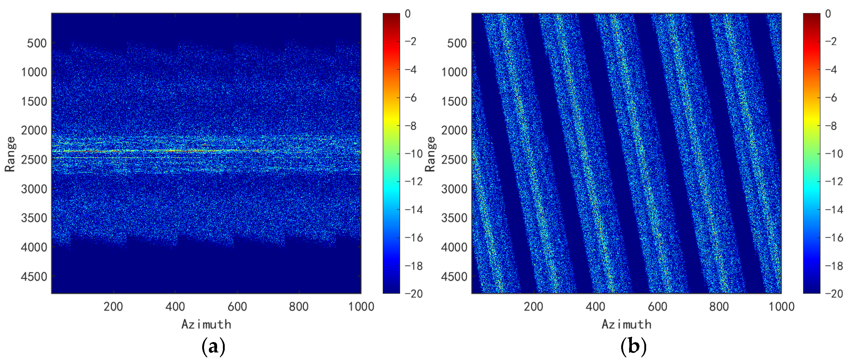
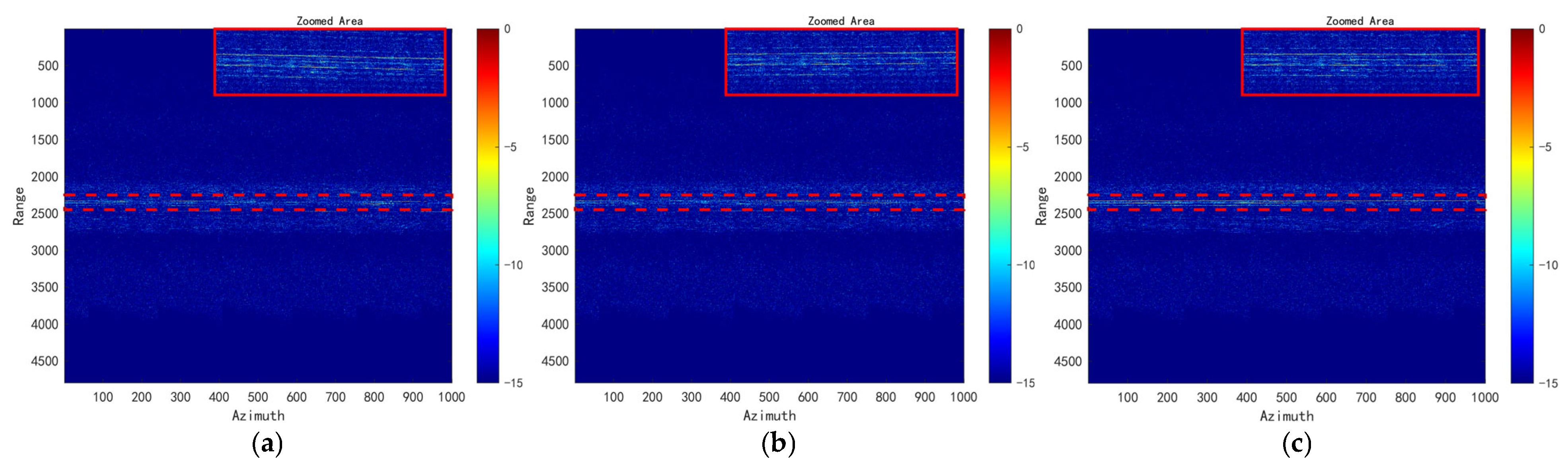
3.5. Field-Measured Data Experiments

In this section, we use the real field-measured data to further validify our proposed method. In the field experiment, a terahertz (THz) radar system was airborne-mounted on an aircraft, while a full-scale satellite model was anchored at a ground-based test site. The aircraft executed a controlled orbital flight pattern around the satellite model, during which the radar illuminated the target and acquired the backscattered echoes. The key parameters of the THz radar used in the experiment are as follows: carrier frequency 220 GHz, PRF 10,000 Hz, sampling rate 480 MHz, and pulse-width 10 us. Artificial injection of high-speed translational motion characteristics into raw radar echoes was necessitated due to the practical limitations in acquiring authentic hypersonic targets during airborne field measurements. The one-dimensional range profiles before and after the injection of high-speed translational motion are shown in Figure 15.

Based on the data with high-speed characteristics, we conduct joint motion compensation with different methods; the one-dimensional range profiles after motion compensation are shown in Figure 15.

Both PSO and GWO were implemented with a population size of 30 and a maximum iteration count of 20. As evidenced by Figure 16 and

Table 3. Synthetic waveform entropy of different one-dimensional range profiles.

	FrFT	FrFT + PSO	The Proposed Method
SWE	8.1633	8.1624	8.1532

, the FrFT-based compensation method exhibited suboptimal phase correction accuracy, while the PSO algorithm failed to converge to a global optimum within the prescribed 20 iterations, resulting in significant degradation in range alignment performance. The iteration curves are shown in Figure 17.

As illustrated in Figure 17, the GWO achieves rapid convergence to the global optimum as early as the fifth iteration, whereas the PSO algorithm exhibits markedly slower convergence dynamics and fails to attain the optimal solution within the predefined maximum iteration threshold.

As illustrated in Figure 18, our proposed method (PM) showcases more resilience to low SNRs compared to the two conventional methods. To quantitatively demonstrate the superiority of our method, quantitative comparisons of image entropy (IE) and image contrast (IC) were conducted for the imaging results in Figure 17 (SNR = 5 dB), while computational efficiency of different methods were recorded in

Table 4. Quantitative comparisons of different imaging methods.

	FrFT	FrFT + PSO	PM
IE	14.521	14.496	14.378
IC	2.9912	3.7731	6.9954
Time Cost	608.7932 s	332.4456 s	341.3764 s

. Furthermore,

Table 5. Quantitative comparisons of different IEs under several SNRs.

SNR (dB)	IE of FrFT	IE of FrFT + PSO	IE of PM
5	14.521	14.496	14.378
0	14.589	14.573	14.542
−5	14.629	14.622	14.61
−10	14.641	14.636	14.628
−15	14.652	14.651	14.65

provides information on different IEs under several low SNRs of different methods.

According to the results shown in Table 5, the PM demonstrates significantly superior imaging quality relative to existing algorithms when the SNR exceeds −15 dB. However, as SNR deteriorates to −15 dB, the imaging performance of PM converges with conventional approaches, exhibiting negligible differences in output fidelity. Consequently, PM should be preferentially deployed in environments where SNR remains above −15 dB. Notwithstanding this operational constraint, PM maintains comparatively enhanced robustness under low-SNR regimes.

4. Discussion

4.1. Discussion of Computational Compexity of PM

As demonstrated in Table 4, the computational time required by the GWO and the PSO algorithms is comparable and significantly lower than that of the global FrFT algorithm. In fact, the major time cost of the FrFT method comes from the search for the optimal angle, the range-dimension FrFT, and the traditional envelope alignment. As for the PM, when the number of pulses chosen for FrFT is small enough, its computational cost primarily comes from the iterative process of the GWO. Let the echo data of size $N\times M$ and $L$ search to find the optimal angle. Meanwhile, assume the number of selected sub-echo pulses is $M/F$, the iteration times is $I$, and the size of the wolf population is $P$. Then, we have the computational complexity of FrFT of $\mathrm{O}((L+2M-1)N\log N)$, while that of PM is $\mathrm{O}(I\cdot P\cdot (M+2N))$. The computational time results shown in Table 4 are obtained on the same computer.

4.2. Discussion of the Technical Difficulties of Large Rotation Angle Scenarios

This paper investigates a THz-ISAR imaging algorithm for high-speed moving space targets, demonstrating promising results. The proposed methodology operates under the constraint of short coherent integration time—implying minimal target rotation angles—thus eliminating the need for compensation of RCM induced by large rotation angles. Notably, terahertz radar emissions feature ultra-wide bandwidth, yielding extremely high range resolution. Consequently, even moderate-sized space targets undergoing minor angular displacements may exhibit significant RCM. Furthermore, the coupling between translation-induced RCM (from high-speed motion) and rotation-induced RCM substantially degrades the efficiency of our joint motion compensation algorithm based on target kinematic parameter estimation.

Therefore, simultaneous mitigation of adverse effects from both high-speed motion and large rotation angles presents two fundamental technical challenges:

• Decoupling translational and rotational motions;
• Precise estimation of translational/rotational parameters.

5. Conclusions

The high rendezvous speed between the radar and targets and the ultra-bandwidth of THz radar induce significant range cell migration and phase errors, resulting in severe defocusing of THz-ISAR images. To address these challenges, this paper establishes a joint motion compensation method. The proposed method shows better imaging quality and less computational complexity with the conventional global FrFT method.

The experimental results indicate that, firstly, the synthetic waveform entropy proposed in this paper shows more robustness with abrupt error when conducing envelope alignment, and it serves well as a fitness function in intelligent optimization algorithms, which provides a new idea for this area. Secondly, when the SNR is higher than −15 dB, the proposed method performs well, and the balance between computational complexity and compensation accuracy can be achieved by choosing an appropriate subset of pulses to achieve coarse estimation and compensation.

Future endeavors will concentrate on enlarging the algorithm’s scope of application, taking the compensation of RCM cause by large rotation angle into consideration. Meanwhile, the research will focus on some targets with more complicated motion characteristics, which cannot simply be described as a third-order velocity–time dependency.

References

1. Xu, G.; Xing, M.D.; Zhang, L.; Duan, J.; Chen, Q.Q.; Bao, Z. Sparse apertures ISAR imaging and scaling for maneuvering targets. IEEE J. Sel. Top. Appl. Earth Obs. Remote Sens. 2014, 7, 2942–2956. [Google Scholar] [CrossRef]
2. Yang, Q.; Fan, L.; Yi, J.; Wang, H. A Novel High-Precision Terahertz Video SAR Imaging Method. IEEE Geosci. Remote Sens. Lett. 2024, 22, 4002405. [Google Scholar] [CrossRef]
3. Yang, L.; Xing, M.; Zhang, L.; Sun, G.C.; Gao, Y.; Zhang, Z.; Bao, Z. Integration of rotation estimation and high-order compensation for ultrahigh-resolution microwave photonic isar imagery. IEEE Trans. Geosci. Remote Sens. 2020, 59, 2095–2115. [Google Scholar] [CrossRef]
4. Ma, J.T.; Gao, M.G.; Guo, B.F.; Dong, J.; Xiong, D.; Feng, Q. High resolution inverse synthetic aperture radar imaging of three-axis-stabilized space target by exploiting orbital and sparse priors. Chin. Phys. B 2017, 26, 108401. [Google Scholar] [CrossRef]
5. Yuan, H.; Zhang, Y.; Li, H.; Chen, J.; Niu, M. Recognition of Space Target Based on GNN under the Condition of Small Samples for ISAR Image. In Proceedings of the 2021 CIE International Conference on Radar (Radar), Haikou, China, 15–19 December 2021; pp. 1366–1370. [Google Scholar]
6. Mostajeran, A.; Naghavi, S.M.; Emadi, M.; Samala, S.; Ginsburg, B.P.; Aseeri, M.; Afshari, E. A High-Resolution 220-GHz Ultra-Wideband Fully Integrated ISAR Imaging System. IEEE Trans. Microw. Theory Tech. 2019, 67, 429–442. [Google Scholar] [CrossRef]
7. Zhang, Y.; Yang, Q.; Deng, B.; Qin, Y.; Wang, H. Experimental Research on Interferometric Inverse Synthetic Aperture Radar Imaging with Multi-Channel Terahertz Radar System. Sensors 2019, 19, 2330. [Google Scholar] [CrossRef] [PubMed]
8. Cooper, K.B.; Dengler, R.J.; Llombart, N.; Thomas, B.; Chattopadhyay, G.; Siegel, P.H. THz Imaging Radar for Standoff Personnel Screening. IEEE Trans. Terahertz Sci. Technol. 2011, 1, 169–182. [Google Scholar] [CrossRef]
9. Ibraheem, I.; Krumbholz, N.; Mittleman, D.; Koch, M. Low-dispersive dielectric reflectors for future wireless terahertz communication systems. In Proceedings of the 32nd International Conference on Infrared and Millimeter Waves and the 15th International Conference on Terahertz Electronics, Cardiff, UK, 2–9 September 2007; pp. 930–931. [Google Scholar]
10. Mcmillan, R.W.; Trussell, C.W.; Bohlander, R.A.; Butterworth, J.C.; Forsythe, R.E. An experimental 225 GHz pulsed coherent radar. IEEE Trans. Microw. Theory Tech. 1991, 39, 555–562. [Google Scholar] [CrossRef]
11. Moll, J.; Schops, P.; Krozer, V. Towards three-dimensional millimeter-wave radar with the bistatic fast-factorized back-projection algorithm-potential and limitations. IEEE Trans. Terahertz Sci. Technol. 2012, 2, 432–440. [Google Scholar] [CrossRef]
12. Caris, M.; Stanko, S.; Palm, S.; Sommer, R.; Wahlen, A.; Pohl, N. 300 GHz radar for high resolution SAR and ISAR applications. In Proceedings of the 16th International Radar Symposium, Dresden, Germany, 24–26 June 2015; pp. 577–580. [Google Scholar]
13. Marchetti, E.; Stove, A.G.; Hoare, E.G.; Cherniakov, M.; Blacknell, D.; Gashinova, M. Space-Based Sub-THz ISAR for Space Situational Awareness—Laboratory Validation. IEEE Trans. Aerosp. Electron. 2022, 58, 4409–4422. [Google Scholar] [CrossRef]
14. Marchetti, E.; Stove, A.G.; Hoare, E.G.; Cherniakov, M.; Blacknell, D.; Gashinova, M. Images of satellite elements with a space-borne Sub-THz ISAR system. In Proceedings of the 18th European Radar Conference, London, UK, 5–7 April 2022; pp. 425–428. [Google Scholar]
15. Yang, Q.; Fan, L.; Li, R.; Gao, C.; Wang, H. Research on the registration and fusion algorithm of terahertz SAR images. Chin. J. Electron. 2025. accepted. [Google Scholar]
16. Ning, Q.; Wang, H.; Yan, Z.; Wang, Z.; Lu, Y. A Fast and Robust Range Alignment Method for ISAR Imaging Based on a Deep Learning Network and Regional Multi-Scale Minimum Entropy Method. Remote Sens. 2024, 16, 3677. [Google Scholar] [CrossRef]
17. Tian, B.; Chen, Z.; Xu, S.; Liu, Y. ISAR imaging compensation of high speed targets based on integrated cubic phase function. In MIPPR2013: Multispectral Image Acquisition, Processing, and Analysis; International Society for Optics and Photonics: Bellingham, WA, USA, 2013; Volume 8917, p. 89170B. [Google Scholar]
18. Zhang, K.-F.; Feng, Z.-H.; Ma, D.-B. Study on a method of compensation for the range profile of high velocity spatial targets. In Proceedings of the 2010 International Conference on Image Analysis and Signal Processing, Hangzhou, China, 9–11 April 2010; pp. 450–453. [Google Scholar]
19. Tian, B.; Lu, Z.; Liu, Y.; Li, X. High velocity motion compensation of IFDS data in ISAR imaging based on adaptive parameter adjustment of matched filter and entropy minimization. IEEE Access 2018, 6, 34272–34278. [Google Scholar] [CrossRef]
20. Sheng, J.; Fu, C.; Wang, H.; Liu, Y. High speed motion compensation for terahertz ISAR imaging. In Proceedings of the 2017 International Applied Computational Electromagnetics Society Symposium (ACES), Suzhou, China, 1–4 August 2017; pp. 1–2. [Google Scholar]
21. Guo, B.; Li, Z.; Xiao, Y.; Shi, L.; Han, N.; Zhu, X. ISAR Speed Compensation Algorithm for High-speed Moving Target Based on Simulate Anneal. In Proceedings of the 2019 IEEE 19th International Conference on Communication Technology (ICCT), Xi’an, China, 16–19 October 2019; pp. 1595–1599. [Google Scholar]
22. Wang, J.; Li, Y.; Song, M.; Huang, P.; Xing, M. Noise Robust High-Speed Motion Compensation for ISAR Imaging Based on Parametric Minimum Entropy Optimization. Remote Sens. 2022, 14, 2178. [Google Scholar] [CrossRef]
23. Chen, R.; Jiang, Y.; Ni, H. Optimal Imaging Time Interval Selection Method for Space Target via Time–Frequency Analysis With Spaceborne ISAR. IEEE Geosci. Remote Sens. Lett. 2023, 20, 4012505. [Google Scholar] [CrossRef]
24. Feng, T.; He, J.; Luo, Y. ISAR Imaging of High Speed Moving Targets Based-on Radon Transform. In Proceedings of the 5th International Conference on Information Assurance and Security, Xi’an, China, 18–20 August 2009; pp. 597–600. [Google Scholar]
25. Chen, C.-C.; Andrews, H.C. Target-Motion-Induced Radar Imaging. IEEE Trans. Aerosp. Electron. Syst. 1980, 16, 2–14. [Google Scholar] [CrossRef]
26. Zhao, J.; Liang, Z. CLEAN and FrFT based Cross-range Scaling Method for ISAR Image. In Proceedings of the International Applied Computational Electromagnetics Society Symposium, Xi’an, China, 16–19 August 2024; pp. 1–3. [Google Scholar]
27. Jiang, Y.; Zhang, Z.; Du, Y. The ISAR range profile compensation of space target based on Chirplet transform. In Proceedings of the 6th Asia-Pacific Conference on Synthetic Aperture Radar, Xiamen, China, 26–29 November 2019; pp. 1–6. [Google Scholar]
28. Zhuang, L.; Lei, W. ISAR echoes coherent processing and imaging using PSO-based adaptive joint time-frequency method. In Proceedings of the 3rd International Asia-Pacific Conference on Synthetic Aperture Radar, Seoul, Republic of Korea, 26–30 September 2011; pp. 1–4. [Google Scholar]
29. Nocedal, J.; Wright, S. Numerical Optimization; Springer: Berlin/Heidelberg, Germany, 2006. [Google Scholar]
30. Shao, S.; Zhang, L.; Liu, H.; Zhou, Y. Spatial-variant contrast maximization autofocus algorithm for ISAR imaging of maneuvering targets. Sci. China Inf. Sci. 2019, 62, 40303. [Google Scholar] [CrossRef]
31. Shao, S.; Zhang, L.; Liu, H.; Zhou, Y. Accelerated translational motion compensation with contrast maximisation optimisation algorithm for inverse synthetic aperture radar imaging. IET Radar Sonar Navig. 2019, 13, 316–325. [Google Scholar] [CrossRef]
Figure 1. Spaceborne THz-ISAR Imaging Scenario.
Remotesensing 17 02152 g001
Figure 2. The processing flowchart of the proposed method.
Remotesensing 17 02152 g002
Figure 3. Simulation results of different target velocity and pulse widths. (a) Vtgt = 500 m/s; (b) Vtgt = 1000 m/s; (c) Vtgt = 1500 m/s.
Remotesensing 17 02152 g003
Figure 4. Pulse compression results of the echo of single scatter with different target velocity. (a) Vtgt = 200 m/s; (b) Vtgt = 500 m/s; (c) Vtgt = 1000 m/s; (d) Vtgt = 1500 m/s; (e) Vtgt = 2000 m/s; (f) Vtgt = 2500 m/s.
Remotesensing 17 02152 g004
Figure 5. FrFT-based target translational velocity estimation result (the first half echo). (a) Before abrupt error elimination; (b) after abrupt error elimination.
Remotesensing 17 02152 g005
Figure 6. Velocity–time relation fitting. (a) Local magnification on the left; (b) comparison of fitting performance between the proposed method and conventional methods, orange color squares represent magnification areas; (c) local magnification on the right.
Remotesensing 17 02152 g006
Figure 7. The point cloud model of satellite.
Remotesensing 17 02152 g007
Figure 8. The range profile before intra-pulse compensation. (a) Range profile, orange color square represent magnification in the area; (b) local magnification.
Remotesensing 17 02152 g008
Figure 9. The range profile after intra-pulse compensation. (a) Range profile, orange color square represent magnification in the area; (b) local magnification.
Remotesensing 17 02152 g009
Figure 10. The aligned range profiles before and after intra-pulse compensation, followed by their ISAR image. (ac) Before intra-pulse compensation, orange color square in (a) represents magnification in the area; (df) after intra-pulse compensation, orange color square in (d) represents magnification in the area.
Remotesensing 17 02152 g010
Figure 11. The electromagnetic satellite model.
Remotesensing 17 02152 g011
Figure 12. The one-dimensional range profile after joint compensation, orange color squares in (a,d,g) represent magnification in the area. (ac) FrFT-based; (df) FrFT + PSO; (gi) proposed method.
Remotesensing 17 02152 g012
Figure 13. The iteration comparison between two algorithms.
Remotesensing 17 02152 g013
Figure 14. The ISAR images created by different methods, orange color squares in (a,c,e) represent magnification in the area. (a,b) FrFT-based; (c,d) FrFT + PSO; (e,f) Proposed.
Remotesensing 17 02152 g014
Figure 15. The one-dimensional range profiles before and after high-speed injection. (a) Before; (b) after.
Remotesensing 17 02152 g015
Figure 16. The one-dimensional profiles created by different methods, red color squares in them represent magnification in the area and the results are shown in Zoomed Area. (a) FrFT-based; (b) FrFT + PSO; (c) proposed.
Remotesensing 17 02152 g016
Figure 17. The iteration comparison between two algorithms.
Remotesensing 17 02152 g017
Figure 18. Imaging results of different methods under several SNRs. (a) FrFT; (b) FrFT + PSO; (c) PM.
Remotesensing 17 02152 g018