Article

Spatial Variation in Coral Diversity and Reef Complexity in the Galápagos: Insights from Underwater Photogrammetry and New Data Extraction Methods

Charles Darwin Research Station, Charles Darwin Foundation, Santa Cruz, Galápagos 200102, Ecuador
*
Author to whom correspondence should be addressed.
Remote Sens. 2025, 17(11), 1831; https://doi.org/10.3390/rs17111831
Submission received: 9 March 2025 / Revised: 3 May 2025 / Accepted: 17 May 2025 / Published: 23 May 2025

Abstract

:
Corals in the Galápagos present diverse reef configurations from biogenic coral reefs to coral communities growing on rocks and sand. These corals have experienced decades of disturbances including recurring El Niño and mass bleaching events. However, traditional methods in ecology have limited capacity in describing coral demographic trends across large spatial scales. Photogrammetry—a form of 3D imaging, has emerged over the past decade as a popular method for benthic surveys. However, the majority of protocols in the field utilize the 2D products of photogrammetry, ignoring overhangs and leaving significant information unexploited. We surveyed seven reef sites across the archipelago using underwater photogrammetry and developed new methods for 3D annotation and fractal dimension calculation. Our findings reveal variation in coral cover, diversity, and structural complexity across the archipelago. Our results align with previous studies in the region and add important information on reef structural complexity which was not measured here before. We release a unique dataset: Galápagos_3D, including seven 3D models and over 17,000 annotated images. This study establishes an important baseline for long-term monitoring, research, and conservation in the Galápagos, potentially informing evidence-based policies and advancing our understanding of coral resilience and recovery.

1. Introduction

The Galápagos archipelago, located in the Eastern Tropical Pacific approximately 1000 km west of Ecuador, is globally renowned for its biodiversity and unique ecological systems [1]. Among its marine ecosystems, coral communities range from those growing on volcanic rocks to fully developed biogenic reefs, such as Wellington Reef in Darwin [2,3]. Despite their relatively small size, these reefs play a crucial role in increasing regional marine connectivity and supporting diverse marine life [4]. However, Galápagos corals face numerous threats including climate change, oscillations in ocean currents, cold-water stress [5], warm-water bleaching events [6,7,8], urban development, tourism impacts [1], intense grazing pressure [9], coral diseases, pollution, habitat destruction [8], and invasive species [10].
Several studies have examined the coral communities in the Galápagos and their responses to environmental disturbances [11]. Over the past four decades, extreme climatic events such as the 1982–1983 and 1997–1998 El Niño events have caused severe coral bleaching and mortality, leading to long-term declines in reef cover and biodiversity [6,7,12]. Additionally, cold-water upwelling events, such as the 2007 La Niña, have further impacted these ecosystems [13,14,15]. More recently, marine heatwaves linked to consecutive El Niño years have raised concerns about the ability of Galápagos corals to withstand recurrent disturbances [13,16].
We started a long-term monitoring project using underwater photogrammetry in seven reef sites around the archipelago in order to document and study the adverse effects of such disturbances on the coral community and reef structural complexity. Photogrammetry is a form of 3D imaging that has been used extensively by marine ecologists in the past decade (e.g., [17,18,19]). Using a series of subsequent images as input, Structure-from-Motion photogrammetry builds a 3D model of the scene and estimates the relative camera locations. The 3D models capture the community structure together with the structural complexity of the site and are thus useful for ecological studies.
Traditionally, measuring coral reef structural complexity and biodiversity was done in situ by divers swimming along transect tapes [20,21,22], and later replaced and supplemented with photo quadrats [23,24], video surveys [22], and photogrammetric methods  [17,25,26,27]. Structural complexity was historically measured in situ using a chain draped over the reef surface and a measuring tape to compare surface contour versus planar distance within a quadrat [20,28], and later along transects [22,29,30,31]. These manual approaches inspired digital methods for calculating structural complexity from high-resolution 3D reconstructions [32]. The first predominant works replicated the rugosity metric in 2D and 3D [33,34,35], followed by more structural complexity metrics such as shelter space, vector dispersion, and fractal dimension [36,37,38,39,40].
Fractal dimension (FD) is a unitless measure of how a structure fills space, based on how spatial details change with measurement scale [41]. While FD has been measured in situ [31,42] and from photogrammetric models of coral colonies and reefs [27,38,39,43,44,45], earlier approaches often relied on top-down projections that neglect overhangs and crevices. Similarly, the majority of biodiversity measurements from photogrammetric models utilize photomosaics [46], which are 2D images generated from a single point of view. Despite offering large spatial coverage (commonly on the order of 100 m2 at sub-centimeter resolution) and enabling advanced analyses via semantic segmentation [47,48], photomosaics overlook the three-dimensional complexity of reefs. Since many cryptic reef organisms inhabit hidden or vertical surfaces [21,49], we found it important to devise a methodology that operates in full 3D.
Our goal was to establish a baseline protocol for long-term monitoring based on photogrammetry in the region. Considering the need to improve cryptic species detection and overhang inclusion into structural complexity quantification, we chose to work with 3D models rather than their 2D counterparts, and introduce two novel analytical approaches:
1.
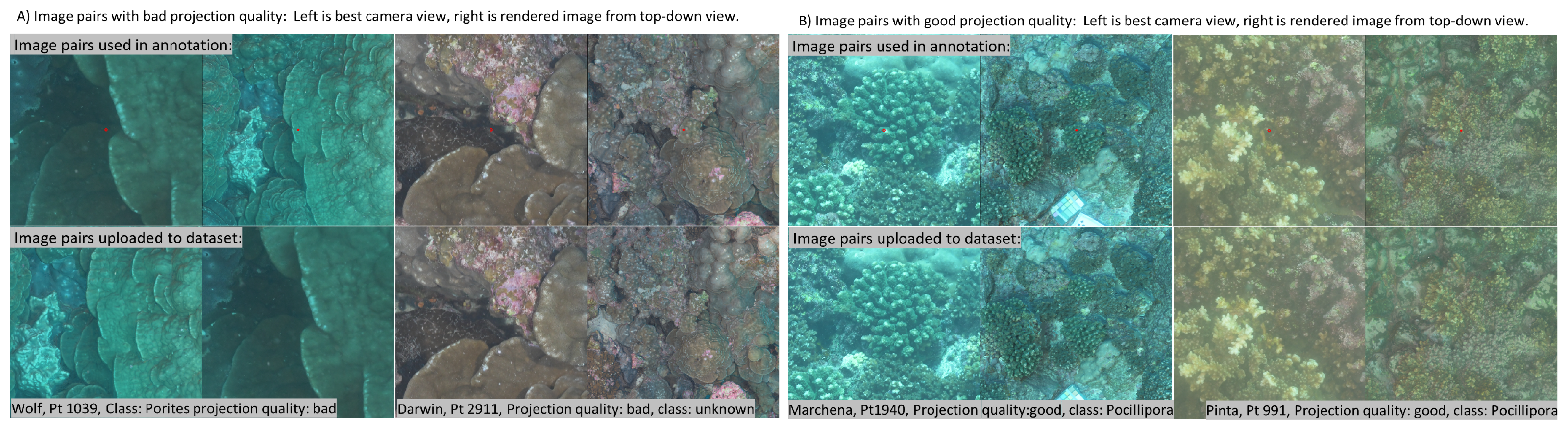
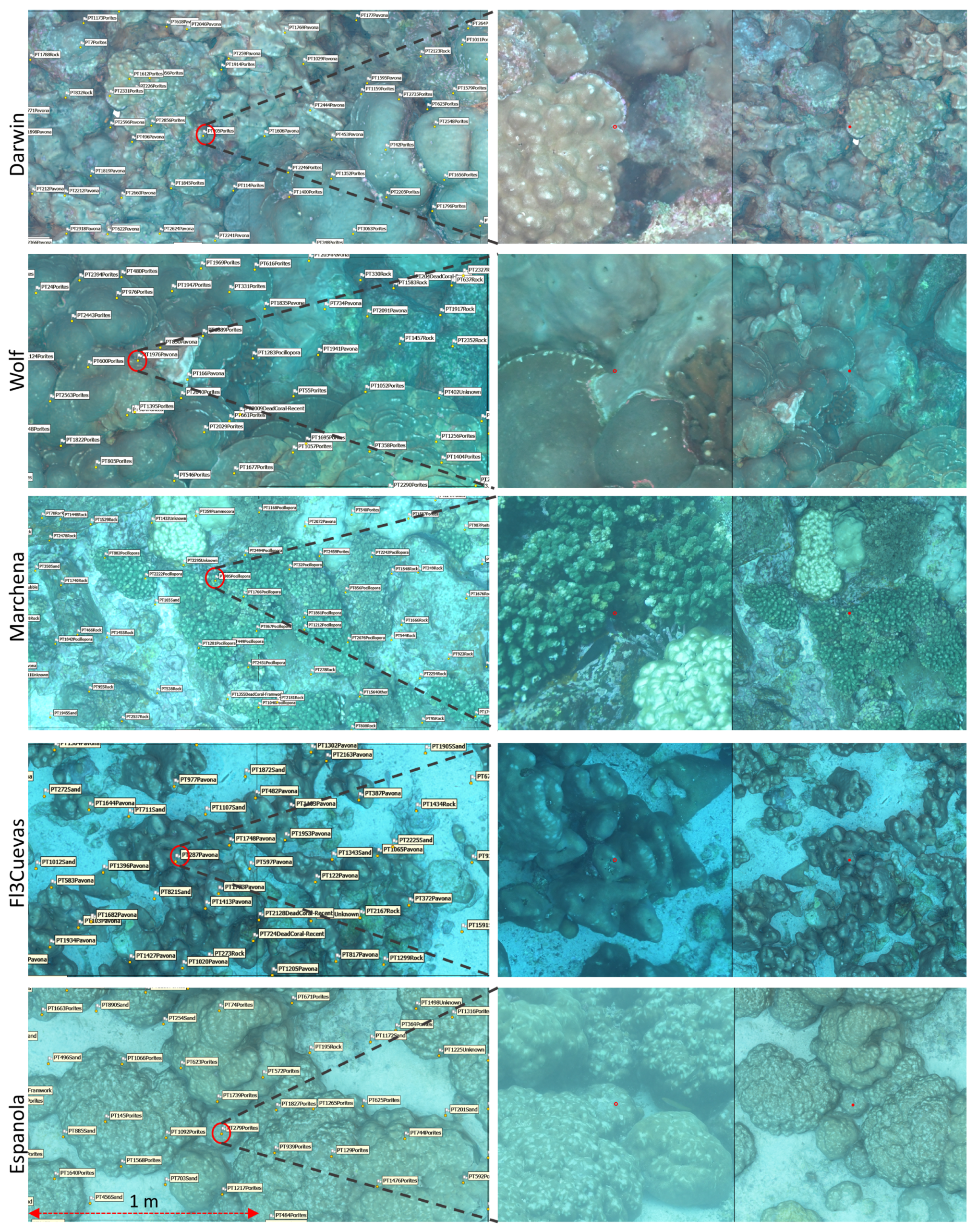
3D point-annotation for benthic classification: We used an image pair for each annotation point including the best camera view and a synthetic view providing the annotator 3D context (See Section 2.5).
2.
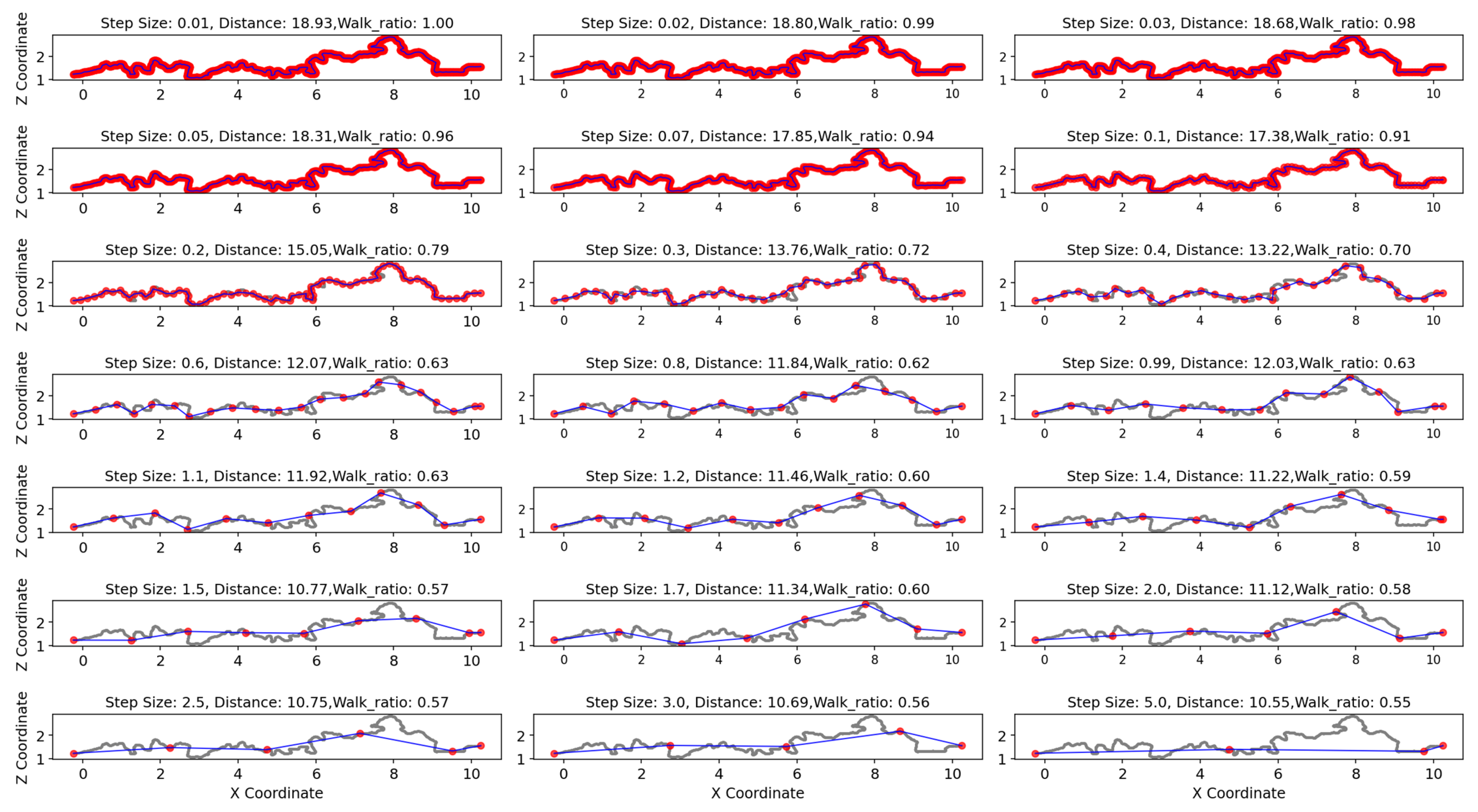
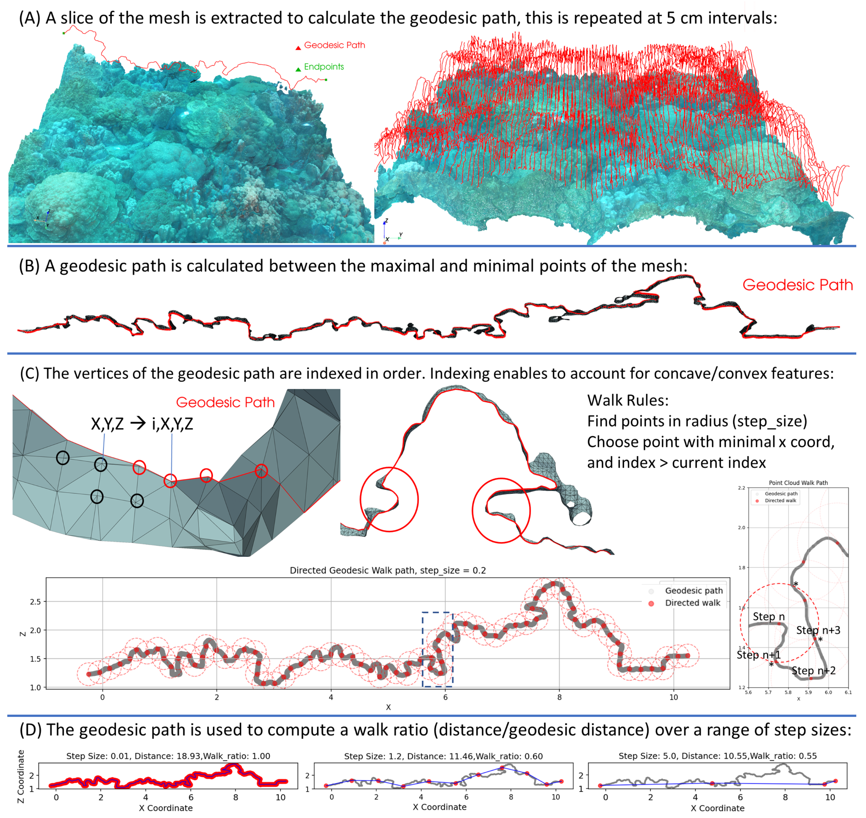
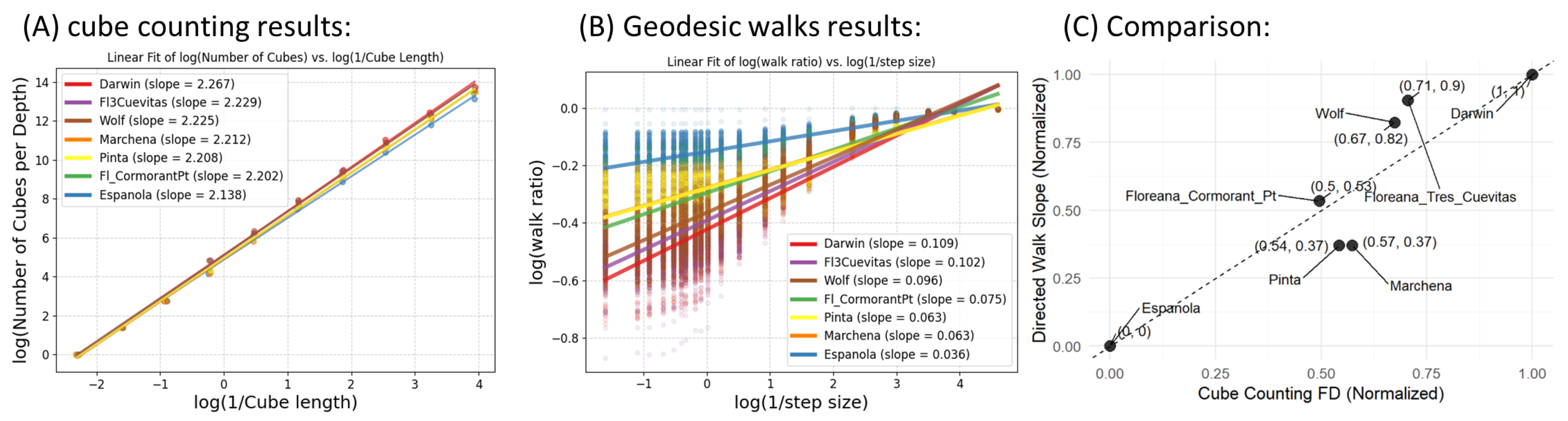
Fractal dimension calculation using directed geodesic walks: These follow a path along a slice of the 3D model without ignoring overhangs thus accounting for full 3D structure (See Section 2.8.2).
We applied these methods to assess coral community structure and reef complexity at seven sites across the Galápagos archipelago and we release our dataset Galápagos_3D (see Appendix A), that includes annotated 3D models useful for research in ecology, computer graphics, Artificial Intelligence (AI), and for informing conservation strategies in the region.

2. Materials and Methods
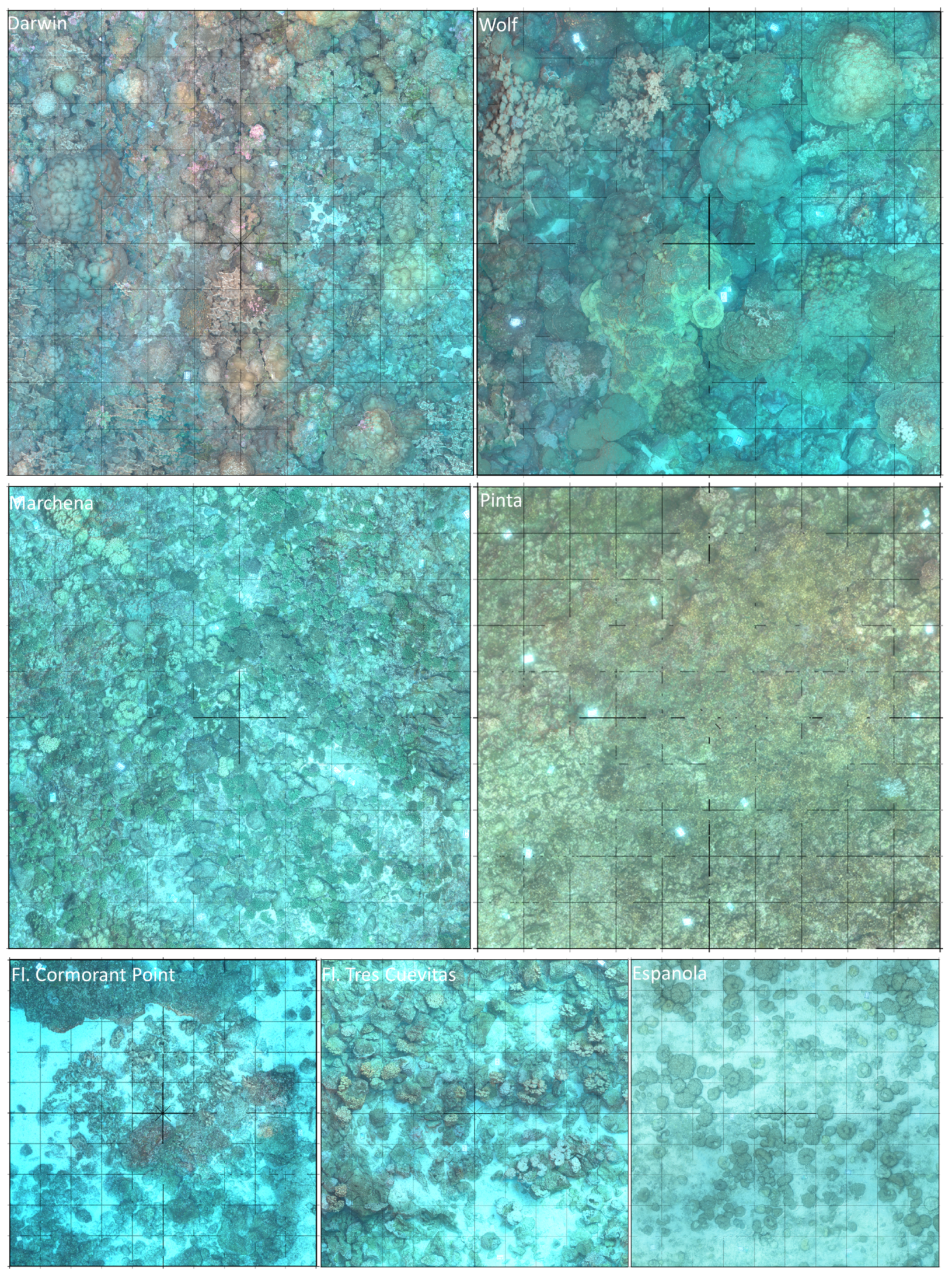
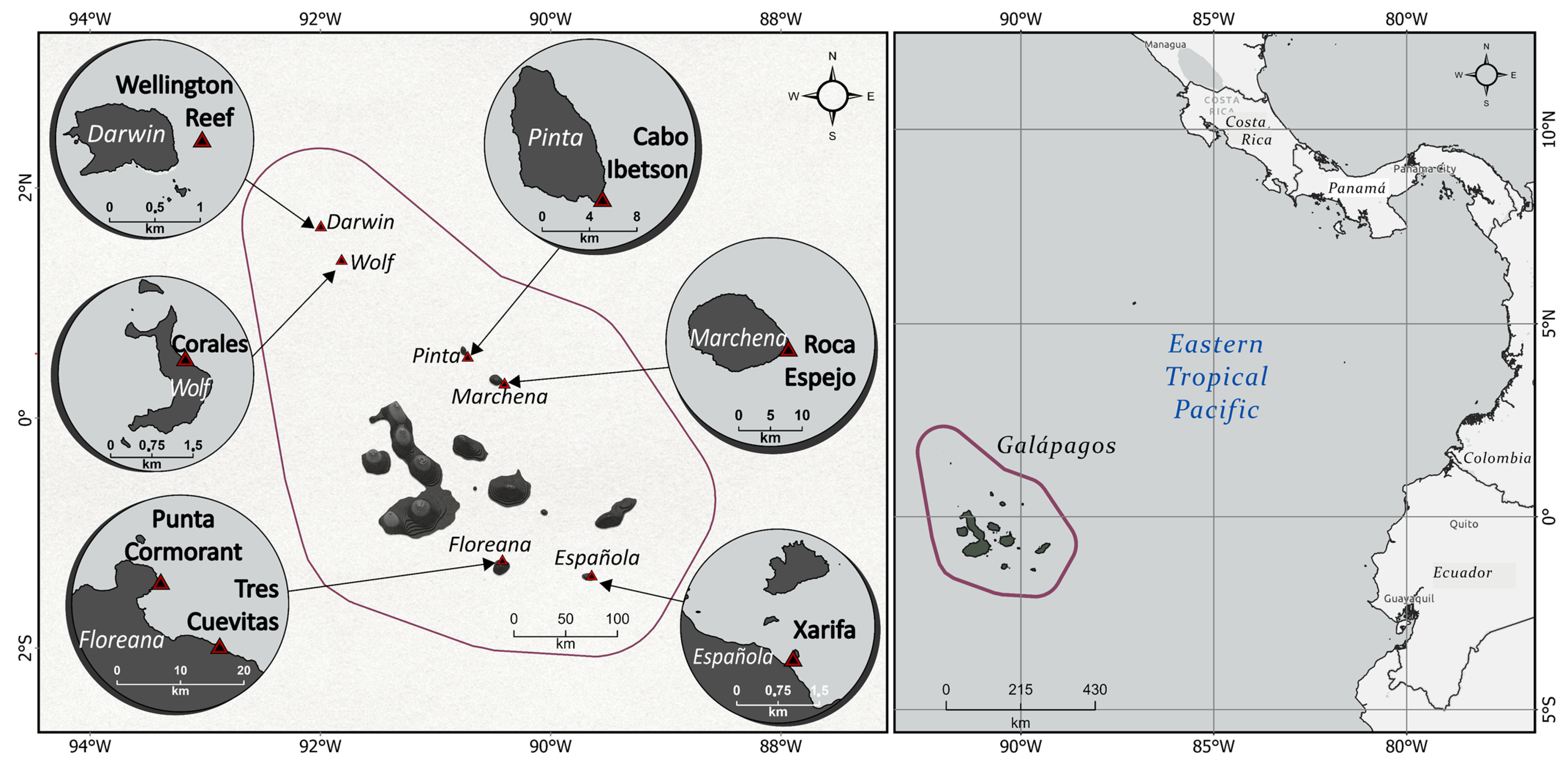
2.1. Study Sites

The locations are distributed throughout the archipelago (Figure 1 and Figure 2) and were selected based on the Charles Darwin Foundation team’s long-term monitoring sites [13] and earlier research in the area [2,4,8,9,12,50]. At each location, we began by examining the area to find a 10 × 10  m2 section featuring the highest coral density and species diversity at a depth of 8–12 m. Balancing these criteria is challenging, as the area with the most coral coverage is often not the most diverse. Additionally, the reef depth varies at each site, as outlined in Table A1. Once the plot was selected and its boundaries marked using a transect tape and a compass, we installed permanent metal stakes at each corner of the plot.

2.2. Image Acquisition and Scene Set-Up

Before image acquisition, we placed a set of photogrammetric markers and color cards in the plot. These are used for scaling the map and assessing the quality of the images in terms of sharpness and illumination during image acquisition and also in post-processing. Moreover, the targets are placed in a way that helps the diver swim in a systematic manner while maintaining overlap between reciprocal legs.
Image acquisition was done using a Nikon D850 DSLR camera with a 35 mm NIKKOR (Nikon, Tokyo, Japan) lens and two Bigblue (Bigblue, Syosset, NY, USA) video lights. Images were acquired from a 2–3 m distance to the substrate at one frame per second. The diver holding the camera swam slowly and steadily while maintaining the camera mostly at a downward-looking angle. Nevertheless, the diver moved the camera around extensive 3D features to capture them from multiple angles of view. The diver swam in a boustrophedonic pattern (lawn mower pattern) across the plot to complete image acquisition from the first distance. Then the diver changed depth to a ∼5 m distance from the substrate and imaged the plot again. Imaging from two distances helps the image alignment process of the 3D reconstruction. For more details on image acquisition and scene set up please see our prior publication [19].
Figure 2. The 3D models from the Galápagos archipelago: Darwin, Wolf, Marchena, Pinta, Floreana, and Española. Each image shows the 3D model of a site. The models are 10 × 10 m 2 . A 1 × 1 m 2 grid is shown in the background of each model.
Remotesensing 17 01831 g002

2.3. 3D Processing

Agisoft Metashape software (version 2.12) was used to reconstruct the 3D models from the series of subsequent images. We used the parameters described in Table S1.
We scaled the models using the photogrammetric targets as scale bars. 10–15 scale bars were defined per model in order to minimize the scaling error. For each scale bar we marked the points of known distance in several input images and entered the known distance value. We marked these points in several images until the scale errors were reduced to sub-centimeter values.

2.4. 3D Model Alignment and Export

After the models were constructed and scaled, we aligned them to the XY axis. This step is important for the structural complexity measurements as we do not want the effect of aspect (slope of the reef— differences in depth between corners of the plot) to affect the measurement. We first fit a plane to each model using the open3D python [51] package. The normal of this plane is used for finding the 3D rotation that aligns the model on the XY plane. We find the rotation matrix of the normal and rotate the model by the inverse. We then use the model’s bounding box to find a translation to the center of the axis (this is detailed in the supplementary code “orient model and set region limits”).
After rotating and translating the model, we build a point cloud from the 3D mesh using a distance-based sampling at 1 cm point density in Metashape. Finally, a 10 m 3 region around the center of the axes was defined and the point clouds were exported for further analysis (cube counting and directed geodesic walks).
The point clouds are released as part of the dataset, please see Appendix A for more details.

2.5. 3D Annotation

We developed a novel approach for annotating 3D models using the best camera view and a synthetic image. First, we use the sparse point cloud generated in image alignment and read it using the open3D library [51]. We build a mesh from these points using the open3D alpha shapes surface reconstruction method. We sample points on this mesh using the open3D sample_points_poisson_disk method where each point has approximately the same distance to the neighbor points. Then we use a KD-tree to find the closest point in the sparse cloud to each of the points. We then read these points back as markers on the 3D model. The number of points per model is determined by measuring the surface area of the model in the region and multiplying it by ten in order to achieve approximately ten points per m2.
For each marker, we extract the image with the smallest reprojection error. Reprojection error is measured by projecting the point from the 3D model (origin point) to the image and back to the 3D model (target point) and calculating the distance between them. After selecting the image with minimal error, it is cropped around the point in 1600 × 1600 pixels. Eventually we resized the images by half to enable their upload resulting in 800 × 800 pixels per image. We also extract a novel view for each point—a synthetic image of the 3D model using a top-down projection. This image is called synthetic because it was never taken by a camera. It is a rendering of the 3D model from a given viewpoint. We used Metashape’s functions to produce these images with each marker as the center of each image and a fixed size of 1600 × 1600 pixels (Figure 3). The advantage of using both images is that the close-up camera image helps to identify the class of the object while the synthetic view helps to put that in context. This is helpful for distinguishing corals such as Porites and Pavona which look similar from a close-up view, but the colonies have different 3D structures.
The pair of images (best camera view and synthetic image) per point was uploaded to Labelbox [52], an online platform for image annotation. The camera view is a close-up on the point while the synthetic image shows the 3D context of the point. Therefore, using the image pairs helps to annotate the points rapidly and accurately.
The annotations are released as part of the dataset, please see Appendix A for more details.

2.6. Classification

A total of 17,807 image pairs were annotated in 12 classes (results are detailed in Table A1): Pavona, Pocillopora, Porites, Psammocora, Rock, Sand, Tubastraea, Caulerpa, Dead Coral—Framework, Dead Coral—Rubble, Other, and Unknown. The class Dead Coral—Framework was used to describe biogenic substrate (coral skeletons that constitute a reef framework) found mostly in Darwin. The class Unknown was used for points where the images (best camera view and synthetic image) did not show the same point. The class Other was used for points that were not in any category such as photogrammetric targets.
The images were annotated by three members of the marine monitoring team of the Charles Darwin Foundation (W.I., F.T., and W.B.-S.) including reviewing all image pairs to validate the classifications. The three annotators were trained in benthic substrate classification and prior to the experiment reviewed different image examples together to achieve uniform classification.
We also used a classification: “Projection quality”, to describe the fit between the synthetic image and the best camera view. When both images showed the same point, we classify it as good, and when the synthetic view does not exactly align with the best camera view, we classify it as bad. This can happen if the 3D point is obscured by an overhang, since the synthetic views are generated only from a top-down view. We used this classification because in the future we aim to use these synthetic images together with the best camera view to train a neural network for coral identification, and using the synthetic views can increases the amount of training data almost twofold. Please see Appendix A for more information on using this data for training a classifier.

2.7. Community Metrics

We calculated the relative abundance of each class per site by dividing the number of observations from each genus by the total number of observations in the model. We calculated the Shannon Diversity index considering only the coral classes: Pavona, Pocillopora, Porites, and Psammocora. We used R Statistical Software (v4.1.2; R Core Team 2021) and the R package vegan [53,54]. Shannon Diversity is calculated as:
H = i = 1 S p i l n ( p i )
where p i is the proportion of species i, and S is the number of species.
We calculated percent coral cover calculating the proportions of four coral classes—Pavona, Pocillopora, Porites, and Psammocora, out of all classes.
We used Principal Component Analysis (PCA) to visualize the difference in community structure on two axes. We omitted the classes Unknown, Other, and Caulerpa from this analysis, thus reducing nine dimensions to two. PCA is a method that identifies the axes (principal components) along which the data has the greatest variance, projecting the data onto these components.

2.8. Structural Complexity Metrics

2.8.1. Fractal Dimension from Cube Counting

We previously worked on cube-counting for assessing fractal dimension of coral reefs and detailed the method extensively [39]. In short, the cube-counting method [55] enables to calculate the fractal dimension of objects as:
F D = lim ϵ 0 log N ( ϵ ) log ( 1 / ( ϵ ) ) ,
where ϵ is the length of the cube and N( ϵ ) is the number of cubes required to cover the object at a given length. N( ϵ ) is calculated for several cube-lengths ( ϵ ) and the fractal dimension is calculated as the slope of the fitted line between log(N( ϵ )) and log(1/ ϵ ).
We take each point cloud and bound it with a minimal bounding cube (∼10 m3). The cube is then divided into 8 equal cubes by dividing each axis. In each iteration, cubes that contain a part of the point cloud are counted (Equation (2)) and used in the next iteration.
For flat shapes, the size of the cube should not affect the measurement while in complex shapes more surface detail is revealed with smaller cube sizes, and the number of cubes increase exponentially when decreasing the cube length. Flat reefs are expected to have lower values close to two, and reefs that are rich in structural features—i.e., structurally complex reefs, are expected to have values closer to three [39].

2.8.2. Fractal Dimension from Directed Geodesic Walks

To calculate structural complexity, we developed an automatic method that takes an input mesh and returns fractal dimension. This is a novel method that elaborates the classic rugosity metric and applies a similar measurement over multiple scales (resolutions) across the full model.
Fractal dimension from geodesic walks = lim ϵ 0 log ( W a l k   r a t i o ) log ( 1 / ( S t e p   s i z e ) )
Walk ratio ( Step size ( r ) ) = Distance traveled Geodesic Distance
The steps below are automatic and do not require intervention. The full code for conducting this analysis is available online. We first construct a mesh from the point cloud using the Open3D Python package (version 0.18). The mesh is then cropped into 5 cm-wide slices with 5 cm intervals along both axes, resulting in approximately 200 slices per site. To measure the structural complexity of these slices we simulate a walk along each slice over a range of step sizes (we used the following step sizes given in meters: = 0.01, 0.02, 0.03, 0.05, 0.07, 0.1, 0.2, 0.3, 0.4, 0.6, 0.8, 0.99, 1.1, 1.2, 1.4, 1.5, 1.7, 2, 2.5, 3, 5). The starting and ending points of the walk are defined as the minimal and maximal coordinates along the slice. Using PyVista [56] python package (version 0.44.1) we calculate the geodesic path: the shortest path along the mesh surface between these points. This path determines the order of points for subsequent walks, therefore we call this method directed geodesic walks. We use the recorded vertices of the geodesic path as a baseline for building a new point cloud by densifying these points. This enab*les us to maintain the order of points rather than just their coordinates for the walk algorithm.
It is crucial to balance the slice width: too wide, and the walk avoids the actual terrain, underestimating complexity; too thin, and the mesh fragments, making the walk ineffective. Moreover, we had several cases (57 out of 29,343) where the walk did not work because the algorithm was unable to find points in the specified step size. We excluded these from the FD assessment.
The algorithm follows two key rules: avoid revisiting previous points (using point indices rather than coordinates), and choose the minimal point on the axis of the walk, for example if the walk is along the x-axis, choose the point with the minimal x coordinate (see Figure 4). For each slice, the walk is conducted twice per step-size: once from start to finish and then in reverse. The average number of steps is recorded, and the walk ratio is calculated as the distance traveled divided by the geodesic path length. A linear model is then fitted to the log relationship between walk ratio and step size for each slice, with the overall score per site being the mean of these measurements.
This method captures structural complexity by observing how the walk ratio decreases with increasing step size (Figure 4). For flat surfaces, step size has little effect, as both small and large steps cover similar distances. For complex surfaces, however, smaller steps traverse more intricate paths, highlighting structural complexity. This difference provides an estimate of the dimension and complexity of the reef structure. The idea is that for complex structures the walk ratio will decrease when increasing the step size. For flat surfaces, the step size r has no influence on the distance of the walk. To portray this, imagine an ant, a horse, and an elephant crossing a surface from start to end. If the surface is flat, they will all travel the same distance. If the surface is wavy, rugged, and complex, the ant will travel a larger distance than the horse and elephant. Measuring how the distance traveled changes by step size gives an estimation of the dimension of the surface and the structural complexity of the reef.

2.9. Estimation of Required Resources

The aforementioned tasks of data collection and analysis include manual labor and computer processing. Image acquisition requires two dives including scene set up and recollection of photogrammetric targets. We dedicated a laptop for this project (ASUS-TEK ROG G18, with intel i9 processor, 64 RAM, and Nvidia RTX 4080 laptop GPU). Building a model on this laptop takes less than 24 h, enabling to view the results rapidly and evaluate if more dives are required for a given site. This is especially important when working in remote areas that require dedicated cruises to reach.
Image annotation was done on the Labelbox online platform [52], that automatically records annotation statistics. Although the full process took us several weeks to complete, the average time per label is between eight and 12 s. A main bottleneck is the internet speed and the time it takes the website to load the image pair for annotation. Given a faster connection, we believe that the average time can be reduced to less than five seconds. Reloading the annotations back to Metashape is done automatically using a python script deployed in Metashape after exporting and parsing the annotations from Labelbox.
The workflow for structural analysis is fully automated, apart from a few manual actions in Metashape software (building point cloud from model and exporting the point cloud). We provide a set of scripts that take the input point cloud and return the FD score from cube counting and geodesic walks.

3. Results

We studied seven reefs using 3D point annotations and structural complexity metrics. All results are summarized in Table A1.

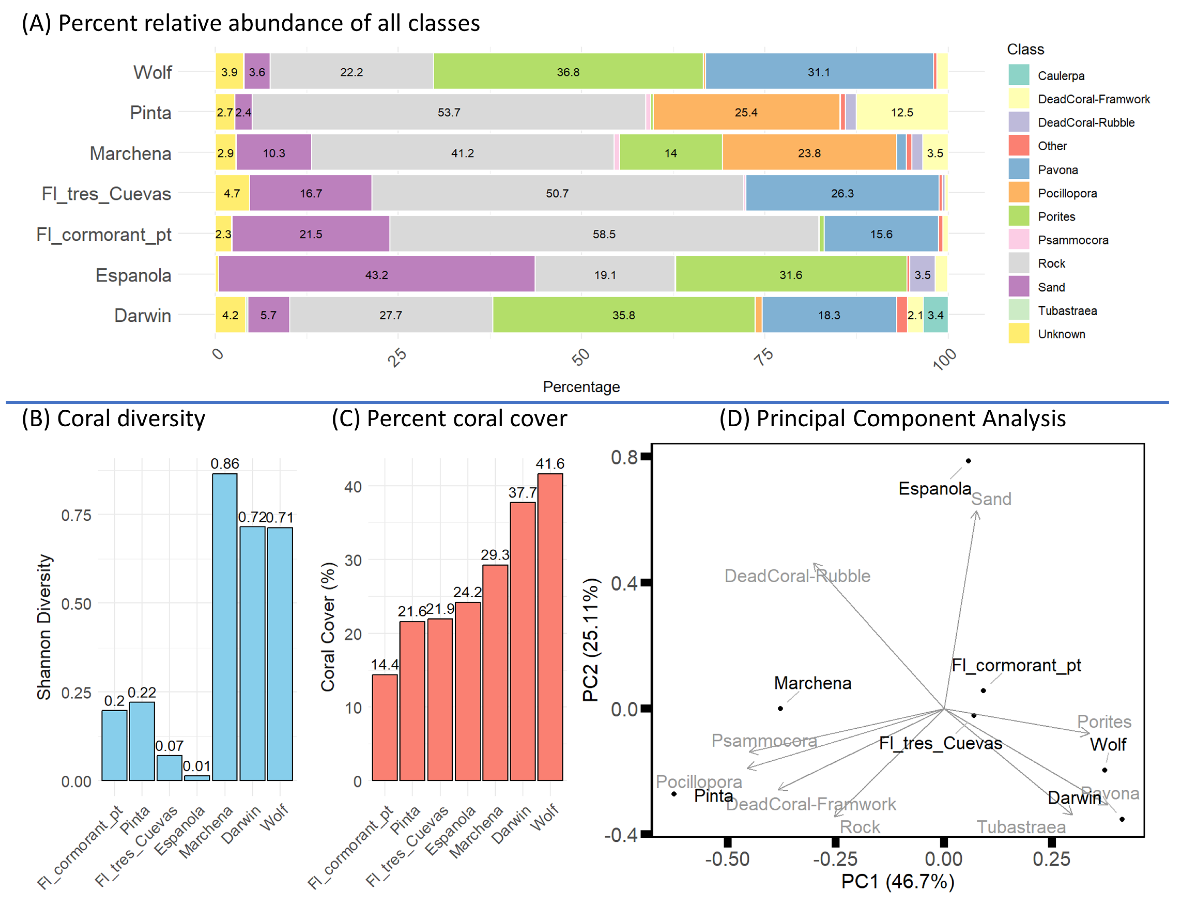
3.1. Community Metrics from 3D Annotations

First, we examined the relative abundance of each class. The results (Figure 5A) show that Darwin (n = 3091) is dominated by Porites (36%) and Pavona (18%). Española (n = 1850) is characterized by Sand (43%) and Porites (32%). Fl_cormorant_pt (n = 2251) is dominated by rock (58%) with contributions from Sand (21%) and Pavona (15%). Fl_tres_Cuevas (n = 2778) shows a high abundance of rock (51%) and Pavona (26%). Marchena (n = 2577) is characterized by rock (41%) and Pocillopora (24%), with higher evenness among coral classes. Pinta (n = 2652) has substantial rock cover (54%) and Pocillopora (25%). Wolf (n = 2608) is dominated by Porites (37%) and Pavona (31%).
Coral diversity (Figure 5B) was calculated based on the coral classes Pavona, Pocillopora, Porites, and Psammocora. The results show that Marchena has the highest diversity (0.87), followed by Darwin and Wolf (0.71/0.72). Española and Fl_tres_cuevas have the lowest diversity. When examining the relative abundance of coral classes, it shows that Española is dominated by Porites, while Fl_cormorant_pt and Fl_tres_cuevas are dominated by Pavona. In contrast, Marchena, Darwin, and Wolf exhibit higher evenness among coral classes.
The results of coral cover per site (Figure 5C) varied from 14% in Fl_cormorant_pt to 42% in Wolf. Darwin had 38% coral cover, while Fl_tres_cuevas, Pinta, and Española had 21–24%. Marchena showed 29% coral cover.

3.2. Multidimensional Scaling

We performed a Principal Component Analysis (PCA) to reduce the dimensionality of the data (Figure 5D) and visualize site similarity and class contributions. The first and second PCs explain 49% and 25% of the variation in the data. Caulerpa class was only apparent in Darwin and Unknown and Other classes are points that were not identified and therefore we dropped them from the PCA.
The PCA biplot (Figure 5D) shows that Darwin and Wolf are close due to their higher proportions of Porites and Pavona. Floreana sites (Fl_tres_cuevas and Fl_cormorant_pt) cluster together and are affected by Pavona, Sand, and Rock. Pinta and Marchena group together due to higher proportions of Pocillopora, and Psammocora, Española is separate from all sites due to the high proportion of Sand.

3.3. Structural Complexity from Cube Counting and Walk Ratios

The results of these two metrics show similar trends. To compare them we normalized them using min-max scaling and plotted them against each other (Figure 6C). Darwin, Fl_tres_cuevas, Wolf, and Espanola maintain their ranks of structural complexity in both methods. However, the sites Marchena and Pinta have the same cube counting results and slightly different walk results. Fl_cormorant_pt has higher Geodesic walk scores than these two sites, but lower FD from cube counting.
These findings emphasize the importance of using complementary metrics to understand reef structural complexity.

4. Discussion

Our results reveal significant variation in coral cover and diversity across sites and differences in structural complexity. Northern sites, such as Darwin and Wolf, exhibited the highest coral cover, primarily dominated by Porites and Pavona species. In contrast, Marchena demonstrated the highest coral diversity, with more evenness among Pavona, Pocillopora, Psammocora, and Porites. Floreana sites had relatively lower coral cover but exhibited high structural complexity, suggesting that these reefs may still provide essential habitat for reef-associated organisms despite their lower coral abundance.
Our findings align with previous research that documented higher coral cover in northern sites and patchier distributions in central and southern locations. Moreover, our study expands upon prior work by incorporating 3D structural complexity assessments that provide a more comprehensive understanding of reef habitat variation. This suggests that our new methods are reliable and valuable for research and monitoring in the region. Moreover, in situ surveys by divers can be biased by the diver. The main advantage of photogrammetry is the ability to analyze the results from the lab in an objective manner.
The results suggest that both geographical location and depth significantly influence coral community composition, although this was not directly tested. The Galápagos archipelago can be divided into five distinct bio-regions based on fish and macro invertebrate community composition [57]. The differences in coral cover and diversity can be linked to their geographic locations as each of these regions is characterized by different physical and biological regimes that can help to explain the observed variation between sites [3]. Importantly, we surveyed only seven plots across the archipelago and more surveys are needed to shed light on the differences within and between islands.
Protocols for annotating photogrammetric models from underwater environments usually use the photomosaic [47,48] which is a 2D representation of the 3D model. We aimed to segment the 3D model in order to obtain samples that are obscured in the photomosaic such as from overhangs and crevices. A similar method for point cloud annotation was previously presented [58,59,60]; however, it requires additional software. Our workflow operates in Metashape and the annotations can be distributed online, e.g., on Labelbox [52]. Moreover, using the synthetic image (the 3D model view) improves the annotation accuracy and speed because it enables to view the point in context while the close-up images facilitate precise identification. Previous research on 3D semantic segmentation of coral reef models was done via deep learning and multi-view images (e.g., [61,62,63,64]). In this work, we have taken the first step toward semantic segmentation of 3D models from the region by compiling a large dataset of annotations (see Appendix A). An important follow up study will focus on training a deep neural net based on the image pairs presented here and testing if including the novel views in training increases the accuracy in predicting benthic classes.
Calculating fractal dimension from geodesic walks is a novel method developed for analyzing wide-scale reef models. Cube counting for fractal dimension was implemented by us previously on smaller models [39]; however, it is less effective for large area models because of their extensive lateral extent and relatively shallow vertical features, which result in larger cube sizes being mostly empty. In Figure 6, A and B appear different primarily due to the range on the y-axis. Darwin, Fl_tres_cuevas, and Wolf exhibit the highest fractal dimension from cube counting and geodesic walks. Española has the lowest slope, suggesting a flatter reef structure. Geodesic walks enable to depict structural complexity in large area models effectively. This is evident in the results (Figure 6C) where geodesic walks maintain similar rank orderings among sites as cube counting. Nevertheless, there are some discrepancies, most notably between Pinta/Marchena and Fl_cormorant_pt. Here, cube counting overestimates structural complexity. The first two are relatively flat models abundant in Pocillopora. On the other hand, Fl_cormorant_pt has an abundance of Pavona colonies scattered across the substrate in different sizes (Figure 2). Cube counting rated these sites high probably because of differences between the small box sizes and the larger ones.
The amount of human input required in this study is relatively low as the majority of methods are automated. Image acquisition is done by divers in situ, taking 1−2 scuba dives. Constructing the models and analyzing them for structural complexity is done automatically with a set of custom python scripts. The image annotation scheme is efficient because it takes only a few seconds for an annotator to classify the image pair in question. Replicating this study in other regions would require basic knowledge of underwater photogrammetry to enable 3D reconstruction and basic proficiency in Python to run the code provided in this work.
Establishing permanent monitoring plots and tracking the fate of single coral colonies over large spatial and temporal extents is one of the crucial next steps in coral reef monitoring and ecology. Expanding our baseline surveys to a continuous monitoring scheme necessitates 3D registration of models from the same site, which is challenging to achieve in the underwater domain [65]. We placed metal stakes in the corners of the plots that can be used as reference points for future surveys and 3D model matching. Once corresponding models of the same site over time are registered (superimposed), the 3D annotation points can be examined in consecutive models, tracking the same point over time. Such direct temporal comparisons can be further automated and facilitated using deep learning. As mentioned above, the dataset generated here (see Appendix A) can be used to train a classifier for classifying the same points over time or new points from more 3D models in the region.
Photogrammetry is becoming one of the most popular tools in the benthic ecology toolbox, with more and more groups adopting 3D imaging protocols to study coral reefs. Nevertheless, the majority of methods use the 2D data: Digital Elevation Models (DEMs) and photomosaics. Considering advances in 3D imaging technologies it is paramount to develop new ways for scientific analysis of 3D data. However, at this point analyzing photomosaics is more pragmatic than analyzing 3D models as there is a plethora of solutions for automatic 2D image segmentation, however there are hardly any tools for 3D segmentation. Moreover, current methods in benthic mosaic analysis enable measuring the sizes of single colonies and how they changes over time [47] (object-based analysis), which our method is lacking (point-based analysis). We believe that in the near future tools will be developed for 3D instance segmentation, which represents the highest level of detail that can be extracted from photogrammetric surveys of the seabed. With regards to structural complexity analysis, in our opinion the method presented here is superior to a DEM based measurement as it accounts for the full 3D structure of the reef as captured by the model rather than reducing a dimension (Z). With this in mind, image acquisition should aim to capture multiple angles of view on the reef rather than having the camera facing only downwards. This helps to ensure that cryptic reef features will show in the 3D reconstruction.

5. Conclusions

Our application of novel photogrammetric techniques represents a significant methodological advancement in Galápagos coral research. Implementing fractal dimension analysis through directed geodesic walks quantifies fine-scale reef complexity across multiple spatial scales, enhancing our ability to compare reefs with different structural compositions and providing a robust metric for monitoring long-term changes in habitat complexity. We release a new dataset: Galápagos_3D, including the 3D models used in this study together with 3D annotations and classified image pairs. This data is useful for studies in ecology and computer graphics such as 3D segmentation from sparse labels via region growing [66].
Additionally, while we documented spatial variation in reef complexity, temporal monitoring is needed to assess long-term resilience. Repeated surveys, particularly following extreme climatic events, will be crucial in understanding whether certain coral communities are developing adaptive responses to recurring stressors. Given the increasing frequency of marine heatwaves and El Niño events, understanding which coral communities are most resilient and why will be critical for conservation planning. Conservation efforts should prioritize sites with high coral cover and structural heterogeneity, as these areas may serve as ecological strongholds in the face of climate change.
Future studies should focus on longitudinal assessments, combining photogrammetry with genetic and physiological analyses to identify potential resilience mechanisms in corals of the Galápagos. Additionally, integrating satellite remote sensing data with underwater photogrammetry could enhance large-scale monitoring efforts, providing a more comprehensive picture of the state of coral ecosystems.
In conclusion, this work demonstrates the application of photogrammetry for coral reef ecology and sets a new standard for reef monitoring in the Galápagos. We report new methods for structural complexity and community composition analysis, and release a new dataset of annotated 3D models. We aim to continue this long-term research effort and contribute to evidence-based conservation policies, ensuring the preservation of these vital ecosystems for future generations.

Supplementary Materials

The following supporting information can be downloaded at: https://www.mdpi.com/article/10.3390/rs17111831/s1; Table S1: 3D Processing Parameters in Metashape software.

Author Contributions

Methodology, software, formal analysis, investigation, data curation, writing—original draft preparation, visualization: M.Y.; Conceptualization, resources, project administration: M.Y., I.K.; Writing—review and editing: M.Y., W.B.-S. and I.K.; Image annotation and validation, fieldwork assistance: F.T., W.B.-S. and W.I.; supervision, funding acquisition: I.K. All authors have read and agreed to the published version of the manuscript.

Funding

Research funding was provided by the Rohr Foundation; Ocean Finance Company; the Paul M. Angell Family Foundation; Lindland; National Geographic; and Ken Collins and Jennifer Mallinson.

Data Availability Statement

The Galápagos_3D dataset including 3D point clouds and point annotations, results of structural complexity calculations, and classified cropped images are available on Zenodo https://doi.org/10.5281/zenodo.14914807(accessed on 15 May 2025). The image-pairs used for annotation are available on request. The code for model alignment on X-Y axis, structural complexity analysis, multi-view image render and export, and loading annotations back to the 3D model is available at https://github.com/MatanYuval/Galapagos-Community-structure (accessed on 15 May 2025).

Acknowledgments

We thank Johny Mazón of the Charles Darwin Foundation for making the map in Figure 1. All authors gratefully acknowledge the Galápagos National Park for authorizing this investigation (research permit: PC-31-24). This publication is contribution number 2711 of the Charles Darwin Foundation for the Galápagos Islands. The authors used chatGPT (version 3.5 and 4) for superficial text editing and for help with writing the scripts to produce the figures. The authors have reviewed and edited the output and take full responsibility for the content of this publication. The authors also used the Metashape online forum to write some of the code for working in Metashape.

Conflicts of Interest

The authors declare no conflicts of interest.

Abbreviations

The following abbreviations are used in this manuscript:
AIArtificial Intelligence
PCAPrincipal Component Analysis
FDFractal Dimension
DEMsDigital Elevation Models

Appendix A. Galápagos_3D Dataset

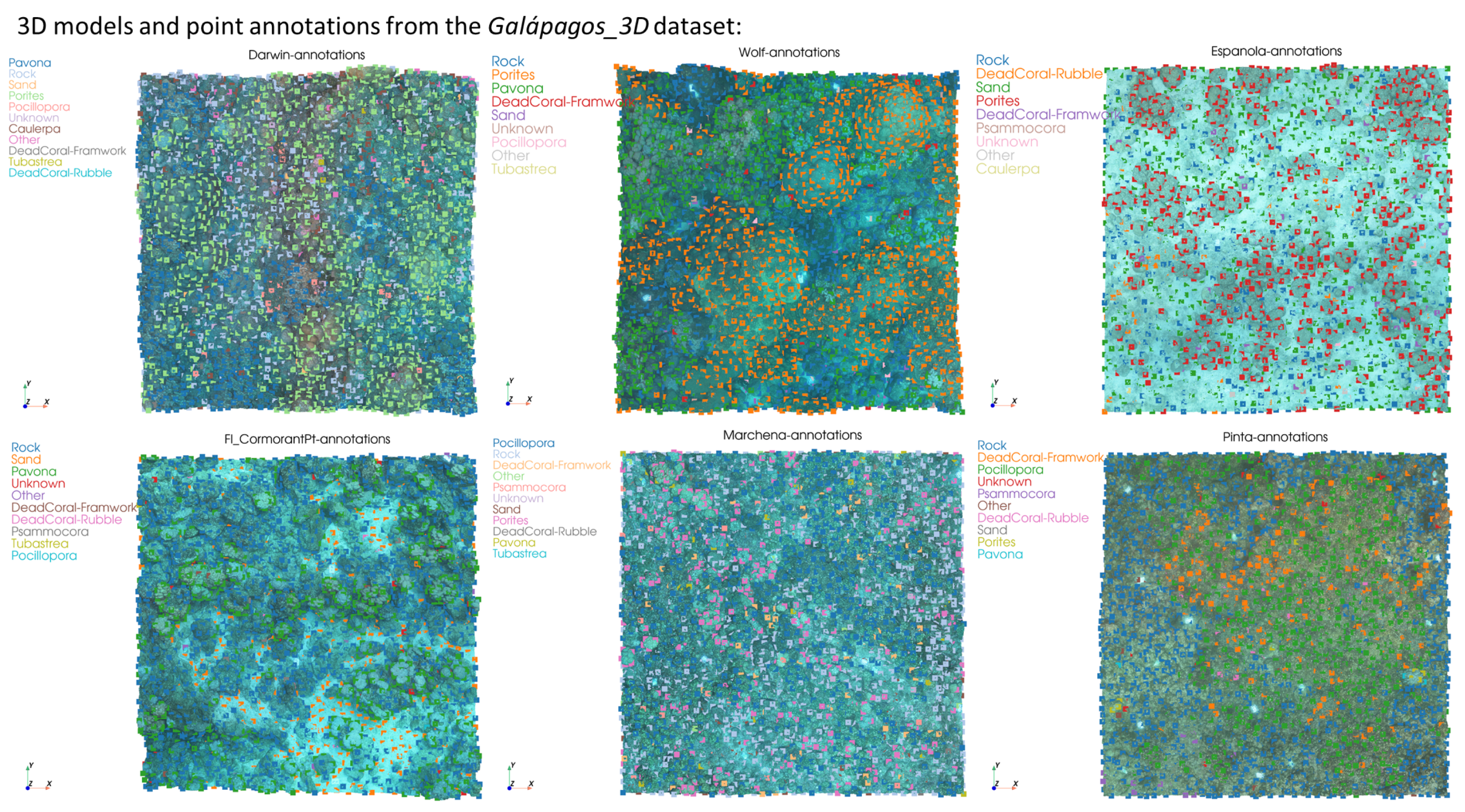
Appendix A.1. Image Annotations

We release the annotated image pairs together with their detailed annotations. The classifications are detailed in the accompanying text file. For each annotation pair we classified the substrate as well as the projection quality. When the images do not show the same exact point, we mark the projection quality as bad. This can happen for two main reasons. Primarily, the synthetic images are rendered from a top-down view, and if the point is on a vertical feature, the synthetic image often does not capture it due to occlusions. In this case we still classify the point but mark the projection as bad. The second reason is where there is a serious offset between the points, and in that case, we classify the point as Unknown and the projection quality as bad. For images where the projection quality is good, both images (the best camera view and the synthetic image) can be used for training algorithms. When the projection quality is bad, use only the best camera view, as the image pair does not depict the same point. Moreover, the original images that were annotated by us had a red circle in their center which was used for classification—we classified the points inside this red circle. In the accompanied dataset we removed these red circles and the classification coordinate is the center pixel, at coordinates 400,400 (the image size was originally 1600 × 1600 but we resized them by half to enable the upload of the large dataset). Figure A1 shows image pairs with good and bad projection accuracy for comparison. The dataset contains 2506 image pairs with bad projection quality out of a total 17,802 image pairs.
Our script for generating the synthetic image uses Metashape’s Graphical User Interface to capture the synthetic views. We generated the synthetic images twice, once for online annotation with red circles in the center, and once without these annotation marks for training data. Due to differences in screen size the footprint of these images has slight variation but their central point is equal, meaning they are valid for use as training data.
Figure A1. Example of annotation dataset and multiple views: (A) Shows examples of bad projection quality from Wolf and Darwin. In the left image pair, the class can still be annotated since it is obvious that the points in both sub images align, but the synthetic image (right in left image pair) is rendered from a top-down view causing an occlusion on the annotation points. In these pairs where the class is not Unknown, the best camera view can be used as training data but not the rendered image. The right image pair shows a bad projection error with the class Unknown, as there is large discrepancy between the best camera view and the rendered image. (B) Shows examples of good projection quality from two sites: Marchena and Pinta. The bottom images are uploaded in the annotation set, without the red markings in the center.
Remotesensing 17 01831 g0a1

Appendix A.2. 3D Models

The point clouds exported from Metashape are uploaded as part of the dataset together with the 3D point annotations. Figure A2 shows several examples of these. To make the figure we used the point cloud and annotation file and the Open3D [51] and PyVista [56] python libraries. The code to reproduce these figures is available in the supplementary code “Create FigS1”. We envision that this data will be used for research on 3D segmentation for example via region growing [66].
Figure A2. 3D point clouds and annotations from the Galápagos_3D dataset: each image shows a 3D point cloud from a different monitoring site with the point annotations overlayed in color. The legend of each model is on the top left side. This helps to visualize differences in abundance patterns between sites, for example, Pinta has a large patch of Pocillopora in the center, and wolf has large colonies of Porites. We envision that this data will be used for research on 3D segmentation for example via region growing [66].
Remotesensing 17 01831 g0a2

Appendix B. Supporting Tables and Figure

Table A1. Summary table of all counts, structural complexity measurements, GPS coordinates, and depth per site.
 Darwin-Wellington ReefEspañola-XarifaFloreana-Tres CuevitasFloreana-Punta CormorantMarchena-Roca EspejoPinta-Cabo IbetsonWolf-Corales
Caulerpa105100000
Dead Coral—Framework663111169033240
Dead Coral—Rubble16512038390
Other4671213181812
Pavona5660731351353812
Pocillopora290106136747
Porites110858401636110961
Rock8553531409131710631423580
Sand1778004634852656493
Tubastraea9011102
Unknown1298130517471101
Psammocora018119180
Cube Counting FD2.2672.1382.2292.2022.2122.2082.225
mean∖_slope0.1089510.0356630.1019560.0748770.0628820.0629780.096196
lacunarity1.4951.6261.9981.6151.4581.5361.684
Surface-Area309185225276258265261
Lat−91.995824−89.644622−90.408089−90.419325−90.401241−90.720945−91.815861
Lon1.67824−1.357863−1.236136−1.2239490.3121620.5442161.386624
Depth15510128812
Figure A3. Fractal dimension from geodesic path: The geodesic path is used to compute a walk ratio (distance/geodesic distance) over a range of step sizes: a walk ratio is determined for each step-size and used to calculate FD for the slice of the mesh. On complex paths, increase in step size causes a decrease in walk ratio.
Remotesensing 17 01831 g0a3

References

  1. Izurieta, A.; Delgado, B.; Moity, N.; Calvopina, M.; Cedeno, Y.; Banda-Cruz, G.; Cruz, E.; Aguas, M.; Arroba, F.; Astudillo, I.; et al. A collaboratively derived environmental research agenda for Galápagos. Pac. Conserv. Biol. 2018, 24, 207. [Google Scholar]
  2. Glynn, P.W.; Wellington, G.M. Corals and Coral Reefs of the Galápagos Islands; University of California Press: Berkeley, CA, USA, 1983. [Google Scholar]
  3. Riegl, B.; Johnston, M.; Glynn, P.W.; Keith, I.; Rivera, F.; Vera-Zambrano, M.; Banks, S.; Feingold, J.; Glynn, P.J. Some environmental and biological determinants of coral richness, resilience and reef building in Galápagos (Ecuador). Sci. Rep. 2019, 9, 10322. [Google Scholar] [CrossRef] [PubMed]
  4. Dawson, T.; Henderson, S.; Banks, S. Galapagos coral conservation: Impact mitigation, mapping and monitoring. Galapagos Res. 2009, 66, 65–74. [Google Scholar]
  5. Foreman, A.D.; Duprey, N.N.; Yuval, M.; Dumestre, M.; Leichliter, J.N.; Rohr, M.C.; Dodwell, R.C.; Dodwell, G.A.; Clua, E.E.; Treibitz, T.; et al. Severe cold-water bleaching of a deep-water reef underscores future challenges for Mesophotic Coral Ecosystems. Sci. Total. Environ. 2024, 951, 175210. [Google Scholar] [CrossRef]
  6. Hickman, C.P., Jr. Evolutionary responses of marine invertebrates to insular isolation in Galapagos. Galapagos Res. 2009, 66, 32–42. [Google Scholar]
  7. Edgar, G.J.; Banks, S.A.; Brandt, M.; Bustamante, R.H.; Chiriboga, A.; Earle, S.A.; Garske, L.E.; Glynn, P.W.; Grove, J.S.; Henderson, S.; et al. El Niño, grazers and fisheries interact to greatly elevate extinction risk for Galapagos marine species. Glob. Change Biol. 2010, 16, 2876–2890. [Google Scholar] [CrossRef]
  8. Glynn, P.W.; Feingold, J.S.; Baker, A.; Banks, S.; Baums, I.B.; Cole, J.; Colgan, M.W.; Fong, P.; Glynn, P.J.; Keith, I.; et al. State of corals and coral reefs of the Galápagos Islands (Ecuador): Past, present and future. Mar. Pollut. Bull. 2018, 133, 717–733. [Google Scholar] [CrossRef]
  9. Glynn, P.W.; Riegl, B.; Purkis, S.; Kerr, J.M.; Smith, T.B. Coral reef recovery in the Galápagos Islands: The northernmost islands (Darwin and Wenman). Coral Reefs 2015, 34, 421–436. [Google Scholar] [CrossRef]
  10. Keith, I.; Dawson, T.P.; Collins, K.J.; Campbell, M.L. Marine invasive species: Establishing pathways, their presence and potential threats in the Galapagos Marine Reserve. Pacific Conserv. Biol. 2016, 22, 377–385. [Google Scholar] [CrossRef]
  11. Feingold, J.S.; Glynn, P.W. Coral research in the Galápagos Islands, Ecuador. In The Galápagos Marine Reserve: A Dynamic Social-Ecological System; Springer: Berlin, Germany, 2013; pp. 3–22. [Google Scholar]
  12. Glynn, P.W. State of coral reefs in the Galápagos Islands: Natural vs anthropogenic impacts. Mar. Pollut. Bull. 1994, 29, 131–140. [Google Scholar] [CrossRef]
  13. Banks, S.; Vera, M.; Chiriboga, A. Establishing reference points to assess long-term change in zooxanthellate coral communities of the northern Galápagos coral reefs. Galapagos Res. 2009, 43–66. [Google Scholar]
  14. Glynn, P.J.; Glynn, P.W.; Riegl, B. El Niño, echinoid bioerosion and recovery potential of an isolated Galápagos coral reef: A modeling perspective. Mar. Biol. 2017, 164, 1–17. [Google Scholar] [CrossRef]
  15. Rhoades, O.K.; Brandt, M.; Witman, J.D. La Niña-related coral death triggers biodiversity loss of associated communities in the Galápagos. Mar. Ecol. 2023, 44, e12767. [Google Scholar] [CrossRef]
  16. Peñaherrera-Palma, C.; Harpp, K.; Banks, S. Rapid seafloor mapping of the northern Galapagos Islands, Darwin and Wolf. Galapagos Res. 2016, 68, 2–9. [Google Scholar]
  17. Burns, J.; Delparte, D.; Gates, R.; Takabayashi, M. Integrating structure-from-motion photogrammetry with geospatial software as a novel technique for quantifying 3D ecological characteristics of coral reefs. PeerJ 2015, 3, e1077. [Google Scholar] [CrossRef]
  18. Ferrari, R.; Figueira, W.F.; Pratchett, M.S.; Boube, T.; Adam, A.; Kobelkowsky-Vidrio, T.; Doo, S.S.; Atwood, T.B.; Byrne, M. 3D photogrammetry quantifies growth and external erosion of individual coral colonies and skeletons. Sci. Rep. 2017, 7, 16737. [Google Scholar] [CrossRef] [PubMed]
  19. Yuval, M.; Alonso, I.; Eyal, G.; Tchernov, D.; Loya, Y.; Murillo, A.C.; Treibitz, T. Repeatable semantic reef-mapping through photogrammetry and label-augmentation. Remote Sens. 2021, 13, 659. [Google Scholar] [CrossRef]
  20. Risk, M.J. Fish diversity on a coral reef in the Virgin Islands. Atoll Res. Bull. 1972, 153, 1–4. [Google Scholar] [CrossRef]
  21. Loya, Y. Plotless and transect methods. In Coral Reefs: Research Methods; UNESCO: Paris, France, 1978; pp. 197–217. [Google Scholar]
  22. Hill, J.; Wilkinson, C. Methods for ecological monitoring of coral reefs. Aust. Inst. Mar. Sci. Townsv. 2004, 117, 27. [Google Scholar]
  23. Laxton, J.; Stablum, W. Sample design for quantitative estimation of sedentary organisms of coral reefs. Biol. J. Linn. Soc. 1974, 6, 1–18. [Google Scholar] [CrossRef]
  24. Ott, B. Community patterns on a submerged barrier reef at Barbados, West Indies. Int. Rev. Gesamten Hydrobiol. Hydrogr. 1975, 60, 719–736. [Google Scholar] [CrossRef]
  25. Ferrari, R.; Lachs, L.; Pygas, D.R.; Humanes, A.; Sommer, B.; Figueira, W.F.; Edwards, A.J.; Bythell, J.C.; Guest, J.R. Photogrammetry as a tool to improve ecosystem restoration. Trends Ecol. Evol. 2021, 36, 1093–1101. [Google Scholar] [CrossRef] [PubMed]
  26. Pavoni, G.; Corsini, M.; Callieri, M.; Palma, M.; Scopigno, R. Semantic segmentation of benthic communities from Ortho-Mosaic maps. Int. Arch. Photogramm. Remote Sens. Spat. Inf. Sci. 2019, XLII-2/W10, 151–158. [Google Scholar] [CrossRef]
  27. Miller, S.; Yadav, S.; Madin, J.S. The contribution of corals to reef structural complexity in Kāne ‘ohe Bay. Coral Reefs 2021, 40, 1679–1685. [Google Scholar] [CrossRef]
  28. Luckhurst, B.; Luckhurst, K. Analysis of the influence of substrate variables on coral reef fish communities. Mar. Biol. 1978, 49, 317–323. [Google Scholar] [CrossRef]
  29. Rogers, C.S.; Garrison, G.; Grober, R.; Hillis, Z.M.; Franke, M.A. Coral Reef Monitoring Manual for the Caribbean and Western Atlantic; Technical Report; Virgin Islands National Park: St. John, United States Virgin Islands, 1994. [Google Scholar]
  30. Rogers, C.S.; Miller, J. Coral bleaching, hurricane damage, and benthic cover on coral reefs in St. John, US Virgin Islands: A comparison of surveys with the chain transect method and videography. Bull. Mar. Sci. 2001, 69, 459–470. [Google Scholar]
  31. Knudby, A.; LeDrew, E. Measuring Structural Complexity on Coral Reefs. In Proceedings of the American Academy of Underwater Sciences 26th Symposium, Dauphin Island, AL, USA, 2007; pp. 181–188. [Google Scholar]
  32. Bryson, M.; Ferrari, R.; Figueira, W.; Pizarro, O.; Madin, J.; Williams, S.; Byrne, M. Characterization of measurement errors using structure-from-motion and photogrammetry to measure marine habitat structural complexity. Ecol. Evol. 2017, 7, 5669–5681. [Google Scholar] [CrossRef]
  33. Friedman, A.; Pizarro, O.; Williams, S.B.; Johnson-Roberson, M. Multi-scale measures of rugosity, slope and aspect from benthic stereo image reconstructions. PLoS ONE 2012, 7, e50440. [Google Scholar] [CrossRef]
  34. Ferrari, R.; McKinnon, D.; He, H.; Smith, R.N.; Corke, P.; González-Rivero, M.; Mumby, P.J.; Upcroft, B. Quantifying multiscale habitat structural complexity: A cost-effective framework for underwater 3D modelling. Remote Sens. 2016, 8, 113. [Google Scholar] [CrossRef]
  35. González-Rivero, M.; Harborne, A.R.; Herrera-Reveles, A.; Bozec, Y.M.; Rogers, A.; Friedman, A.; Ganase, A.; Hoegh-Guldberg, O. Linking fishes to multiple metrics of coral reef structural complexity using three-dimensional technology. Sci. Rep. 2017, 7, 13965. [Google Scholar] [CrossRef]
  36. Hylkema, A.; Debrot, A.O.; Osinga, R.; Bron, P.S.; Heesink, D.B.; Izioka, A.K.; Reid, C.B.; Rippen, J.C.; Treibitz, T.; Yuval, M.; et al. Fish assemblages of three common artificial reef designs during early colonization. Ecol. Eng. 2020, 157, 105994. [Google Scholar] [CrossRef]
  37. Urbina-Barreto, I.; Chiroleu, F.; Pinel, R.; Fréchon, L.; Mahamadaly, V.; Elise, S.; Kulbicki, M.; Quod, J.P.; Dutrieux, E.; Garnier, R.; et al. Quantifying the shelter capacity of coral reefs using photogrammetric 3D modeling: From colonies to reefscapes. Ecol. Indic. 2021, 121, 107151. [Google Scholar] [CrossRef]
  38. McCarthy, O.S.; Smith, J.E.; Petrovic, V.; Sandin, S.A. Identifying the drivers of structural complexity on Hawaiian coral reefs. Mar. Ecol. Prog. Ser. 2022, 702, 71–86. [Google Scholar] [CrossRef]
  39. Yuval, M.; Pearl, N.; Tchernov, D.; Martinez, S.; Loya, Y.; Bar-Massada, A.; Treibitz, T. Assessment of storm impact on coral reef structural complexity. Sci. Total Environ. 2023, 891, 164493. [Google Scholar] [CrossRef]
  40. Aston, E.A.; Duce, S.; Hoey, A.S.; Ferrari, R. A Protocol for Extracting Structural Metrics From 3D Reconstructions of Corals. Front. Mar. Sci. 2022, 9, 854395. [Google Scholar] [CrossRef]
  41. Mandelbrot, B.B.; Passoja, D.E.; Paullay, A.J. Fractal character of fracture surfaces of metals. Nature 1984, 308, 721–722. [Google Scholar] [CrossRef]
  42. Nash, K.L.; Graham, N.A.; Wilson, S.K.; Bellwood, D.R. Cross-scale habitat structure drives fish body size distributions on coral reefs. Ecosystems 2013, 16, 478–490. [Google Scholar] [CrossRef]
  43. Reichert, J.; Backes, A.R.; Schubert, P.; Wilke, T. The power of 3D fractal dimensions for comparative shape and structural complexity analyses of irregularly shaped organisms. Methods Ecol. Evol. 2017, 8, 1650–1658. [Google Scholar] [CrossRef]
  44. Fukunaga, A.; Burns, J.H. Metrics of coral reef structural complexity extracted from 3D mesh models and digital elevation models. Remote Sens. 2020, 12, 2676. [Google Scholar] [CrossRef]
  45. Torres-Pulliza, D.; Dornelas, M.A.; Pizarro, O.; Bewley, M.; Blowes, S.A.; Boutros, N.; Brambilla, V.; Chase, T.J.; Frank, G.; Friedman, A.; et al. A geometric basis for surface habitat complexity and biodiversity. Nat. Ecol. Evol. 2020, 4, 1495–1501. [Google Scholar] [CrossRef]
  46. Remmers, T.; Grech, A.; Roelfsema, C.; Gordon, S.; Lechene, M.; Ferrari, R. Close-range underwater photogrammetry for coral reef ecology: A systematic literature review. Coral Reefs 2024, 43, 35–52. [Google Scholar] [CrossRef]
  47. Pavoni, G.; Corsini, M.; Ponchio, F.; Muntoni, A.; Edwards, C.; Pedersen, N.; Sandin, S.; Cignoni, P. TagLab: AI-assisted annotation for the fast and accurate semantic segmentation of coral reef orthoimages. J. Field Robot. 2022, 39, 246–262. [Google Scholar] [CrossRef]
  48. Remmers, T.; Boutros, N.; Wyatt, M.; Gordon, S.; Toor, M.; Roelfsema, C.; Fabricius, K.; Grech, A.; Lechene, M.; Ferrari, R. RapidBenthos: Automated segmentation and multi-view classification of coral reef communities from photogrammetric reconstruction. Methods Ecol. Evol. 2024, 16, 427–441. [Google Scholar] [CrossRef]
  49. Kornder, N.A.; Cappelletto, J.; Mueller, B.; Zalm, M.J.; Martinez, S.J.; Vermeij, M.J.; Huisman, J.; de Goeij, J.M. Implications of 2D versus 3D surveys to measure the abundance and composition of benthic coral reef communities. Coral Reefs 2021, 40, 1137–1153. [Google Scholar] [CrossRef]
  50. Vera, M.; Banks, S. Health status of the coral communities of the northern Galapagos Islands Darwin, Wolf and Marchena. Galapagos Res. 2009, 66, 3–5. [Google Scholar]
  51. Zhou, Q.Y.; Park, J.; Koltun, V. Open3D: A Modern Library for 3D Data Processing. arXiv 2018, arXiv:1801.09847. [Google Scholar]
  52. Labelbox, Online. 2025. Available online: https://labelbox.com/ (accessed on 16 May 2025).
  53. R Core Team. R: A Language and Environment for Statistical Computing; R Foundation for Statistical Computing: Vienna, Austria, 2021. [Google Scholar]
  54. Oksanen, J.; Simpson, G.L.; Blanchet, F.G.; Kindt, R.; Legendre, P.; Minchin, P.R.; O’Hara, R.; Solymos, P.; Stevens, M.H.H.; Szoecs, E.; et al. Vegan: Community Ecology Package; R Package Version 2.6-8. 2024. Available online: https://CRAN.R-project.org/package=vegan (accessed on 16 May 2025).
  55. Schroeder, M. Fractals, Chaos, Power Laws: Minutes from an Infinite Paradise; W.H. Freeman: New York, NY, USA, 1991. [Google Scholar]
  56. Sullivan, C.B.; Kaszynski, A. PyVista: 3D plotting and mesh analysis through a streamlined interface for the Visualization Toolkit (VTK). J. Open Source Softw. 2019, 4, 1450. [Google Scholar] [CrossRef]
  57. Edgar, G.; Banks, S.; Fariña, J.; Calvopiña, M.; Martínez, C. Regional biogeography of shallow reef fish and macro-invertebrate communities in the Galapagos archipelago. J. Biogeogr. 2004, 31, 1107–1124. [Google Scholar] [CrossRef]
  58. Petrovic, V.; Vanoni, D.J.; Richter, A.M.; Levy, T.E.; Kuester, F. Visualizing high resolution three-dimensional and two-dimensional data of cultural heritage sites. Mediterr. Archaeol. Archaeom. 2014, 14, 93–100. [Google Scholar]
  59. Fox, M.D.; Carter, A.L.; Edwards, C.B.; Takeshita, Y.; Johnson, M.D.; Petrovic, V.; Amir, C.G.; Sala, E.; Sandin, S.A.; Smith, J.E. Limited coral mortality following acute thermal stress and widespread bleaching on Palmyra Atoll, central Pacific. Coral Reefs 2019, 38, 701–712. [Google Scholar] [CrossRef]
  60. Pavoni, G.; Pierce, J.; Edwards, C.B.; Corsini, M.; Petrovic, V.; Cignoni, P. Integrating Widespread Coral Reef Monitoring Tools for Managing both Area and Point Annotations. Int. Arch. Photogramm. Remote Sens. Spat. Inf. Sci. 2024, 48, 327–333. [Google Scholar] [CrossRef]
  61. King, A.; Bhandarkar, S.M.; Hopkinson, B.M. Deep Learning for Semantic Segmentation of Coral Reef Images Using Multi-View Information. In Proceedings of the IEEE Conference on Computer Vision and Pattern Recognition Workshops, Long Beach, CA, USA, 16–17 June 2019; pp. 1–10. [Google Scholar]
  62. Pierce, J.; Butler, M.J., IV; Rzhanov, Y.; Lowell, K.; Dijkstra, J.A. Classifying 3-D models of coral reefs using structure-from-motion and multi-view semantic segmentation. Front. Mar. Sci. 2021, 8, 706674. [Google Scholar] [CrossRef]
  63. Marlow, J.; Halpin, J.E.; Wilding, T.A. 3D photogrammetry and deep-learning deliver accurate estimates of epibenthic biomass. Methods Ecol. Evol. 2024, 15, 965–977. [Google Scholar] [CrossRef]
  64. Sauder, J.; Banc-Prandi, G.; Meibom, A.; Tuia, D. Scalable semantic 3D mapping of coral reefs with deep learning. Methods Ecol. Evol. 2024, 15, 916–934. [Google Scholar] [CrossRef]
  65. Lechene, M.A.; Figueira, W.F.; Murray, N.J.; Aston, E.A.; Gordon, S.E.; Ferrari, R. Evaluating error sources to improve precision in the co-registration of underwater 3D models. Ecol. Inform. 2024, 81, 102632. [Google Scholar] [CrossRef]
  66. Zhan, Q.; Liang, Y.; Xiao, Y. Color-based segmentation of point clouds. Laser Scanning 2009, 38, 155–161. [Google Scholar]
Figure 1. Overview of the Galápagos Archipelago and study sites: Map of the Galápagos Archipelago with the study sites shown in red triangles within the marine reserve (outer line). The Galápagos Archipelago lies on the equator in the Eastern Tropical Pacific approx. 1000 km off the coast of Ecuador.
Remotesensing 17 01831 g001
Figure 3. Method for 3D annotation using the best camera and synthetic views: Each row is from a different site. The left images show a 2 × 1 m close-up of the 3D model with the markers and their identities. The right images show the pair of images that were used to annotate a marker. For each point, two images are extracted: a 1600-pixel crop around the annotation point on the best image that depicts the point, and a novel synthetic image from a top-down view of the point.
Remotesensing 17 01831 g003
Figure 4. Method for calculating fractal dimension from geodesic walks: (A) A slice is extracted from the 3D model (left) and used to calculate the geodesic path between start and end points. This process is repeated at 5 cm intervals to extract approximately 100 slices per side (top, right). The model is then rotated 90° around the z-axis, and the process is repeated to capture slices on both axes. (B) A profile of a geodesic path extracted from the 3D model. (C) Close-up of a mesh slice and its geodesic path. The path connects vertices, assigning a walk order by index (ordinal), not just position. The algorithm selects the next vertex within a radius (step size) based on the minimal coordinate along the walk axis. The bottom image illustrates sequential walk steps with red circles indicating the step-size radius. The right image, a close-up of the dashed-blue region, highlights step n and potential next points within the radius (asterisks). Point n+1 is chosen by minimal x-coordinate. (D) A walk ratio is determined for each step-size and used to calculate FD for the slice of the mesh. On complex paths, increase in step size causes a decrease in walk ratio. The overall score per site is the average FD of 200 slices ((A), right).
Remotesensing 17 01831 g004
Figure 5. Annotation results: (A) Stacked bar chart of the percent relative abundance of benthic classes in Darwin (n = 3091), Española (n = 1850), Fl_cormorant_pt (n = 2251), Fl_tres_cuevas (n = 2778), Marchena (n = 2577), Pinta (n = 2652), and Wolf (n = 2608). (B) Shannon diversity index ( H ) of coral genera based on the classes Pavona, Pocillopora, Porites, and Psammocora. (C) Percentage of coral cover calculated as the proportion of annotations from Pavona, Pocillopora, Porites, and Psammocora out of all annotations (D) PCA biplot of benthic class composition, with PC1 and PC2 explaining 47% and 25% of the variance.
Remotesensing 17 01831 g005
Figure 6. Relationships between structural complexity methods: (A) Linear fit of log (Number of Cubes) vs. log (1/Side Length), showing slopes for each site. The slopes represent fractal dimensions estimated through cube counting, with values ranging from 2.138 in Española to 2.267 in Darwin. (B) Linear fit of log (Walk Ratio) vs. log (1/Step Size) was calculated for each slice of the mesh, we then calculated the average slope for each site (shown in legend). The slopes represent the Fractal dimension from geodesic walk ratios, ranging from 0.036 in Española to 0.109 in Darwin. (C) Cube Counting FD plotted against Geodesic Walk FD. The data was normalized between 0−1, and the order of the sites is mostly conserved, illustrating a strong correlation.
Remotesensing 17 01831 g006
Disclaimer/Publisher’s Note: The statements, opinions and data contained in all publications are solely those of the individual author(s) and contributor(s) and not of MDPI and/or the editor(s). MDPI and/or the editor(s) disclaim responsibility for any injury to people or property resulting from any ideas, methods, instructions or products referred to in the content.

