Article

Comparative Analysis of Trophic Status Assessment Using Different Sensors and Atmospheric Correction Methods in Greece’s WFD Lake Network

by
Vassiliki Markogianni
1,*,
Dionissios P. Kalivas
2,
George P. Petropoulos
3,
Rigas Giovos
2 and
Elias Dimitriou
1
1
Institute of Marine Biological Resources and Inland Waters, Hellenic Centre for Marine Research, 46.7 km of Athens-Sounio Avenue, 19013 Anavissos, Attica, Greece
2
Department of Natural Resources Management and Agricultural Engineering, Agricultural University of Athens, 75 Iera Odos, 11855 Athens, Attica, Greece
3
Department of Geography, Harokopio University of Athens, El. Venizelou 70, Kallithea, 17671 Athens, Attica, Greece
*
Author to whom correspondence should be addressed.
Remote Sens. 2025, 17(11), 1822; https://doi.org/10.3390/rs17111822
Submission received: 2 April 2025 / Revised: 9 May 2025 / Accepted: 20 May 2025 / Published: 23 May 2025

Abstract

Today, open-source Cloud Computing platforms are valuable for geospatial image analysis while the combination of the Google Earth Engine (GEE) platform and new satellite launches greatly facilitate the monitoring of national-scale lake Water Quality (WQ). The main aim of this research is to assess the transferability and performance of published general, natural-only and artificial-only lake WQ models (Chl-a, Secchi Disk Depth-SDD- and Total Phosphorus-TP) across Greece’s WFD (Water Framework Directive) lake sampling network. We utilized Landsat (7 ETM +/8 OLI) and Sentinel 2 surface reflectance (SR) data embedded in GEE, while subjected to different atmospheric correction (AC) methods. Subsequently, Carlson’s Trophic State Index (TSI) was calculated based on both in situ and modelled WQ values. Initially, WQ models employed both DOS1-corrected (Dark Object Subtraction 1; manually applied) and GEE-retrieved respective SR data from the year 2018. Double WQ values per lake station were inserted in a linear regression analysis to harmonize the AC differences, separately for Landsat and Sentinel 2 data. Yielded linear equations were accompanied by strong associations (R2 ranging from 0.68 to 0.98) while modelled and GEE-modelled TSI values were further validated based on reference in situ WQ datasets from the years 2019 and 2020. The values of the basic statistical error metrics indicated firstly the increased assessment’s accuracy of GEE-modelled over modelled TSIs and then the superiority of Landsat over Sentinel 2 data. In this way, the hereby adopted methodology was evolved into an efficient lake management tool by providing managers the means for integrated sustainable water resources management while contributing to saving valuable image pre-processing time.

1. Introduction

Nowadays, the World’s lakes’ greatest threat is commonly known: the so-called eutrophication, which is greatly connected to an increase in nutrients, mainly phosphorus and nitrogen [1]. WQ is the most significant indicator of a water body’s state, while its assessment requires the continuous monitoring of mainly physico-chemical and biological elements [2]. Based on the crucial roles that lakes play in human society (climate regulation, drinking water supply, wildlife habitats, recreation, and tourism) and the negative consequential impacts of water eutrophication on lake environments, it is inherently essential to monitor and assess lakes’ water trophic status [3]. Moreover, the quantification of inland waters’ trophic status offers valuable information concerning water resource management decisions [3]. TSI is the most widely used indicator for assessing the trophic state of inland waters [4,5]; it was initially proposed by [4] and is based on chlorophyll-a (Chl-a), Secchi disk depth (SDD) and total phosphorus (TP) measurements [4]. Even though trophic status assessment of numerous inland waters worldwide is conducted using various approaches [6,7,8], the traditional method includes in situ sampling and laboratory analysis [9]. However, those methods are time- and labor-intensive particularly when large-scale investigations are needed [10]. Today, through the evolution of Remote Sensing (RS) techniques, satellite images provide invaluable information facilitating the assessment of different WQ components, such as the total suspended matter (TSM) and colored dissolved organic matter (CDOM) content, the SDD, and the Chl-a concentration [11,12,13,14,15,16]. Furthermore, due to their wide coverage, RS expedites regional and large-scale WQ monitoring [17,18,19].
However, computing WQ properties (and by extension TSI) from RS images may also become time-demanding and sophisticated because of the processing data chain, particularly a great-scale WQ assessment and high-frequency time series demand [20]. Today, platforms for big Earth Observation (EO) Data Management and Analysis have emerged as computational solutions that provide functionalities for big EO data management, storage and access including processing without downloading big amounts of datasets and provision of images of certain pre-processing levels [21]. Ref. [21] overviewed and compared seven platforms (GEE, Sentinel Hub-SH-, Open Data Cube-ODC-, System for Earth Observation Data Access, Processing and Analysis for Land Monitoring-SEPAL-, open EO, JEODPP and pipsCloud) among certain functionalities including data, processing and physical infrastructure abstraction, open governance, reproducibility of science, infrastructure replicability, processing and storage scalability, data access interoperability and extensibility. Based initially on this survey and then on studies conducted by [22,23,24], it was concluded that GEE outperforms the available cloud computing systems and was proven the most significant cloud-processing platform for the RS community due to its ease of use and maturity.
The GEE platform has changed the traditional RS data processing mode [24] as it consists of a multi-petabyte analysis-ready data catalog while allowing users to compute massive-scale analysis and accomplish multiple RS and geospatial tasks at remarkable speeds and scales [25]. The data repository of GEE includes publicly available geospatial datasets, along with observations from a variety of satellite and aerial imaging systems in both optical and non-optical wavelengths, environmental variables, weather forecasts, land cover and other datasets [25]. In addition to this, the satellite data catalog is updated on a daily basis with around 6000 new image scenes.
Numerous recent studies have recorded applications of WQ monitoring of inland waters based on GEE [26,27,28,29,30,31,32,33,34,35,36]. Of particular importance though is the utilized AC methods. Precise AC is crucial for applications where small differences in SR are significant, such as retrieval of WQ parameters in water [37,38,39]. Furthermore, AC enables direct comparison between different image dates and different sensors. Based on this advantage, the hereby utilized sensors are the Landsat 7 ETM +, Landsat 8 OLI and Sentinel 2. Landsat (30 m spatial resolution) and Sentinel 2 (10–60 m spatial resolution) missions provide fine-scale spatial data and have been reported to be suitable for the quantification of multiple WQ indices in freshwater lakes and reservoirs [14,15,40,41,42,43,44]. Landsat sensors’ temporal resolution is 16 days while Landsat 7 ETM + and 8 OLI together provide one (1) satellite image every 8 days [1]. The Sentinel 2 mission carries two satellites—Sentinel 2A and Sentinel 2B—equipped with identical Multispectral Instruments (MSI)-, the revisit frequency of each satellite is 10 days while the combined revisit is equal to 5 days. However, those sensors differ in their orbital spatial and spectral configuration, resulting in affecting the recorded radiometric values; hence, different sensor data need to be processed independently to be less influenced [45].
All in all, this work constitutes an effort to initially assess certain WQ elements and then calculate the water trophic state (TSI) throughout 50 natural and artificial lakes, constituting the WFD National Lake Monitoring Network in Greece. The hereby adopted methodological scheme includes the exploration of the performance of published empirically developed WQ quantitative models of Chl-a [13], SDD and TP [16] when employing GEE-retrieved reflectance values which are corrected using different AC methods.
More particularly, in situ measurements of Chl-a, SDD and TP from the year 2018 were paired twice with concurrent satellite reflectance values derived from combined Landsat 7 ETM +/8 OLI (first dataset) and Sentinel 2 MSI (second dataset) images. The two-fold match initially concerns the reflectance derived from manually downloaded and pre-processed images with the DOS1 method and then the GEE-derived reflectance (from the exact same satellite images) which are delivered corrected using LaSRC (Land Surface Reflectance Code), LEDAPS (Ecosystem Disturbance Adaptive Processing System) and Sen2Cor (Sentinel 2 Atmospheric Correction) correction algorithms. Linear regression analysis among the resulting WQ values (at the WFD sampling sites) was then conducted to highlight and potentially harmonize inherent differences primarily between the differently atmospherically corrected reflectance values and, afterward, among the different sensors used.
Moreover, the available in situ WQ data for the years 2019 and 2020 were paired with concurrent GEE-derived reflectance values at WFD sites to additionally test the strength of the WQ models for estimating Chl-a, SDD and TP concentrations. Lastly, respective in situ TSIs were utilized as further validation of the remote-sensed ones to definitely conclude the models’ suitability for the trophic status assessment of optically diverse inland waters at a national scale (Greece).
In view of the above, the present study’s main target is to derive the water trophic state of Greece’s lakes efficiently through the GEE cloud-based platform which is conducted by fulfilling the following objectives: (1) calculate WQ elements across Greek studied lakes and further validate the hereby utilized empirically developed WQ models based on available in situ data; (2) test the spatiotemporal performance of WQ models when employing GEE-retrieved SR that is corrected with different AC methods; (3) harmonize the differences by developing sensor-specific GEE-WQ models individually for Landsat and Sentinel 2 sensors; and (4) further validate the modelled and GEE-modelled TSI values based on error metrics.

2. Materials and Methods
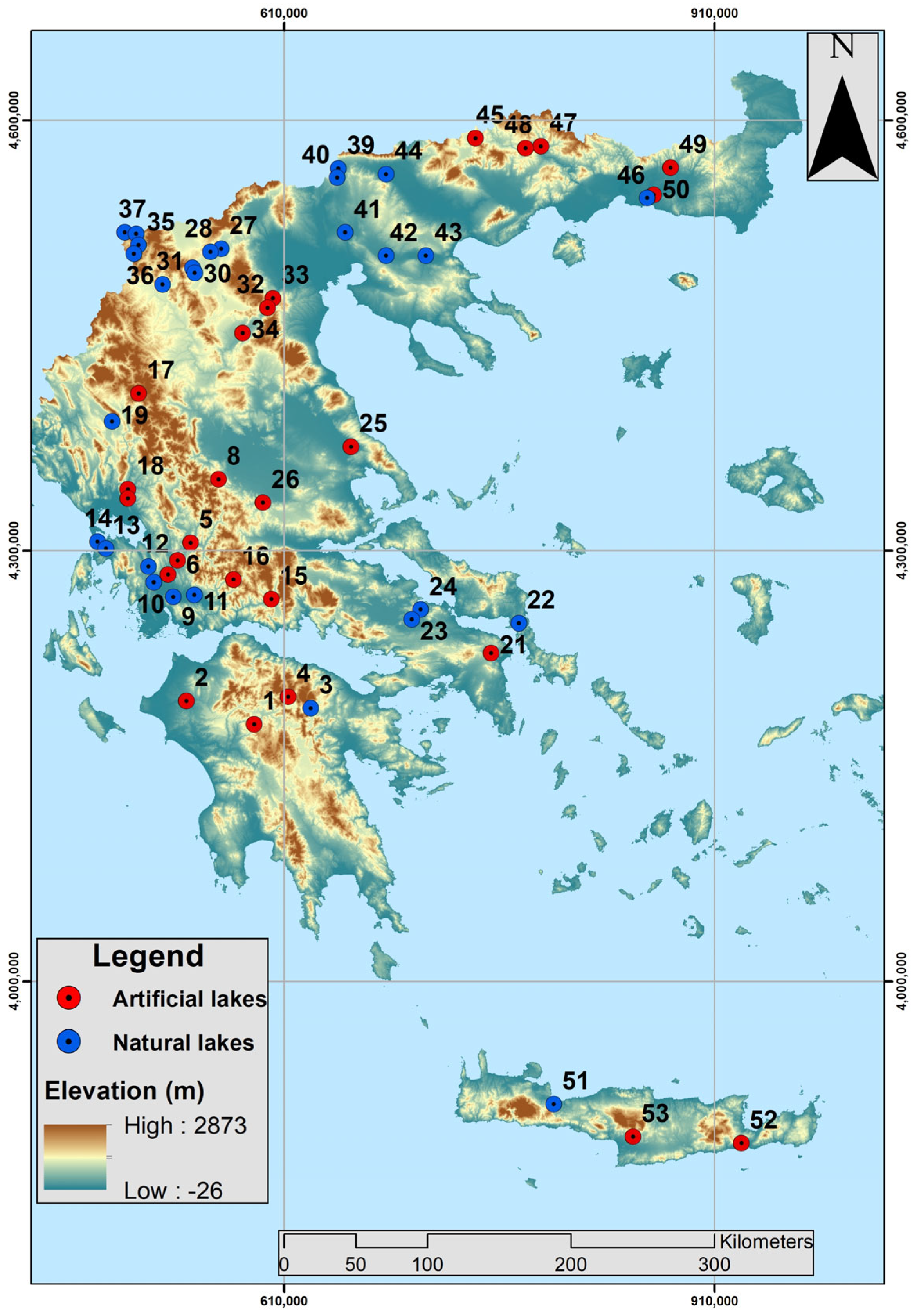
2.1. In Situ Data

Directive 2000/60/EC, establishing a framework for Community action in the field of water policy, also known as the Water Framework Directive, is the primary legislation for water protection in Europe. It applies to inland waters (lakes and rivers), transitional waters (lagoons and estuaries), coastal surface waters, and groundwater. By Joint Ministerial Decision 140384/2011, the Goulandris Natural History Museum/Hellenic Biotope-Wetland Centre (GNHM/EKBY) was designated as the responsible authority for monitoring 53 stations (27 surveillance; 26 operational) in 50 Greek lakes, natural and artificial. At the majority of the lakes, only one sampling station is detected, except for transboundary lakes (Megali Prespa, Mikri Prespa, and Doirani), where two sampling stations are located (Figure 1; Table 1). Regular sampling is conducted at lake monitoring stations to assess biological, physicochemical, and hydromorphological water quality parameters. Additionally, analyses of these parameters are performed, followed by data processing and synthesis, quality index calculations, and classification of the ecological status of the lakes. In situ dataset used in this study concern the freely accessible data (https://wfd.ekby.gr/apotelesmata/biologika-physikochimika-dedomena/ (accessed on 18 January 2022); in Greek) including measured values of Chl-a and TP concentrations and SDD measurements on several dates during the years 2018, 2019 and 2020. Concerning the phytoplankton (Chl-a) analysis, monthly sampling is conducted at lake monitoring stations during the warm period of the year, with a single integrated water sample taken from the euphotic zone of the lake. In deep reservoirs, the Mediterranean assessment method “New Mediterranean Assessment System Reservoirs Phytoplankton (NMASRP)” [46] is applied. In natural lakes, the HeLPhy (Hellenic Lake Phytoplankton) assessment method [47] is used. Water sampling for the analysis of chemical and physicochemical elements is conducted simultaneously with phytoplankton sampling during the warm period and seasonally throughout the rest of the year. At each monitoring station water transparency is measured using the Secchi disk. In the laboratory, after collecting water samples from the euphotic zone, total phosphorus (mg/L or μg/L) is determined using the ascorbic acid method (APHA 4500) [48]). More detailed information about the sampling and analysis methods for each quality parameter is available on the institution’s site (https://wfd.ekby.gr/parakolouthisi-limnon/methodologia/ (accessed on 18 January 2022); in Greek).
Furthermore, a summary of descriptive statistics of in situ measurements is presented in Supplementary Files (Table S1). Based on mean values of all three parameters, a slight water quality deterioration is observed from 2018 to 2019, followed by an improvement in 2020.

2.2. Satellite Imagery and Pre-Processing

Refs [45,50] confirmed that when processing each satellite image separately and conducting independent training—similar to our approach—the impact of differences in recorded radiometric values among various satellite sensors is minimized. Based on this rationale, independent processing of Landsat and Sentinel 2 images throughout hereby research, eliminated the need for resampling.
Acquired SR products from the GEE repository included Sentinel 2 MSI (Level-2A SR data) and Landsat 7 ETM +/8 OLI multispectral images (Collection 1 Level 1-precision and terrain correction-Tier 1; SR data). The time window for satellite acquisition from GEE was set to ±7 days in relation to the sampling date as proposed by [36]. GEE-derived reflectance values are available and atmospherically corrected with different AC algorithms depending on the sensor; Landsat 8 OLI and Landsat 7 ETM + images are corrected using the Land Surface Reflectance Code (LaSRC) and the Ecosystem Disturbance Adaptive Processing System (LEDAPS) methods, respectively. LaSRC AC is performed using a radiative transfer model, auxiliary atmospheric data from MODIS (Moderate Resolution Imaging Spectroradiometer) and utilizes the coastal aerosol band for aerosol inversion tests. LEDAPS algorithm calculates the radiative transfer for atmospheric data from MODIS and NCEP (National Centers for Environmental Prediction) [51]. Sentinel 2 products in GEE are corrected with the Sentinel 2 Atmospheric Correction (Sen2Cor) algorithm. Sen2Cor algorithm is a combination of state-of-the-art techniques for performing AC together with a scene classification algorithm, which allows detection of clouds, snow and cloud shadows and generation of a classification map. This map consists of 3 different classes for clouds (including cirrus), 6 different classifications for shadows, cloud shadows, vegetation, not vegetated, water and snow [52]; accessed on 10 July 2022. Then, SR values of several dates during the years 2018, 2019 and 2020 were extracted through the GEE platform at the points where the sampling stations are located (Figure 1), initially from Landsat (8 OLI; 7 ETM +) and then from Sentinel 2 MSI images. Since the reflectance fraction in GEE is scaled by 10,000, values were divided by 10,000 to obtain 0–1 reflectance values from the respective cells.
Concerning the manual pre-processing of satellite images, Landsat 7 ETM + and 8 OLI images of 2018 were downloaded from the USGS (United States Geological Survey) Data Centre (https://earthexplorer.usgs.gov/ (accessed on 5 February 2020)) in the context of the study conducted by [16]. Moreover, Sentinel 2 images of 2018 were also downloaded from the Copernicus open access hub (Sentinel-2|Copernicus Data Space Ecosystem https://dataspace.copernicus.eu/explore-data/data-collections/sentinel-data/sentinel-2 (accessed on 10 July 2022)). Manually downloaded Sentinel 2 and Landsat images were subjected to the same pre-processing procedure, as described in [16] and more particularly, they were imported in the semi-automatic classification plugin (SCP) of the free and open-source cross-platform desktop Quantum Geographic Information System (Q-GIS), v. 3.6.3-Noosa to perform: (a) conversion of images from digital numbers (DN) to top-of-atmosphere reflectance (TOA), (b) AC by using the DOS1 method [53], applied to all bands except for thermal ones, and (c) the creation of a band stack set for each image. DOS1 method minimizes the additive effect of the atmosphere caused by haze. The main assumption is that dark objects represent 1% of reflectance while they are identified by an area with clear water in deep lakes or by the histogram method, which selects the DN of haze from the DN frequency histogram of an image [54]. The selection of the DOS method was maintained after the completion of the studies conducted by [13,16] (where the WQ models were initially developed) and was further reinforced based on the studies carried out by [37,55]. Refs. [37,55] intercompared five (5) [6S (atmospheric correction method of the second simulation of satellite in the solar spectrum); FLAASH (Fast Line-of-sight Atmospheric Analysis of Spectral Hypercube); ATCOR (Atmospheric Correction for Airborne and Satellite Imaging); DOS and ELM (empirical line method)] and three (3) [DOS; ATCOR3; MODTRAN5 (MODerate resolution atmospheric TRANsmission) different AC methods, respectively. Ref. [37] overviewed those methods over sand, artificial surface, grass and water while they concluded that DOS performed well over water, as it indicated higher differences than the physical methods and is proposed as a good choice for SR estimation of dark surfaces such as water. Ref. [55] evaluated the aforementioned methods across certain Spanish lakes and ponds and concluded that DOS performed better than the others, reporting the lowest errors.

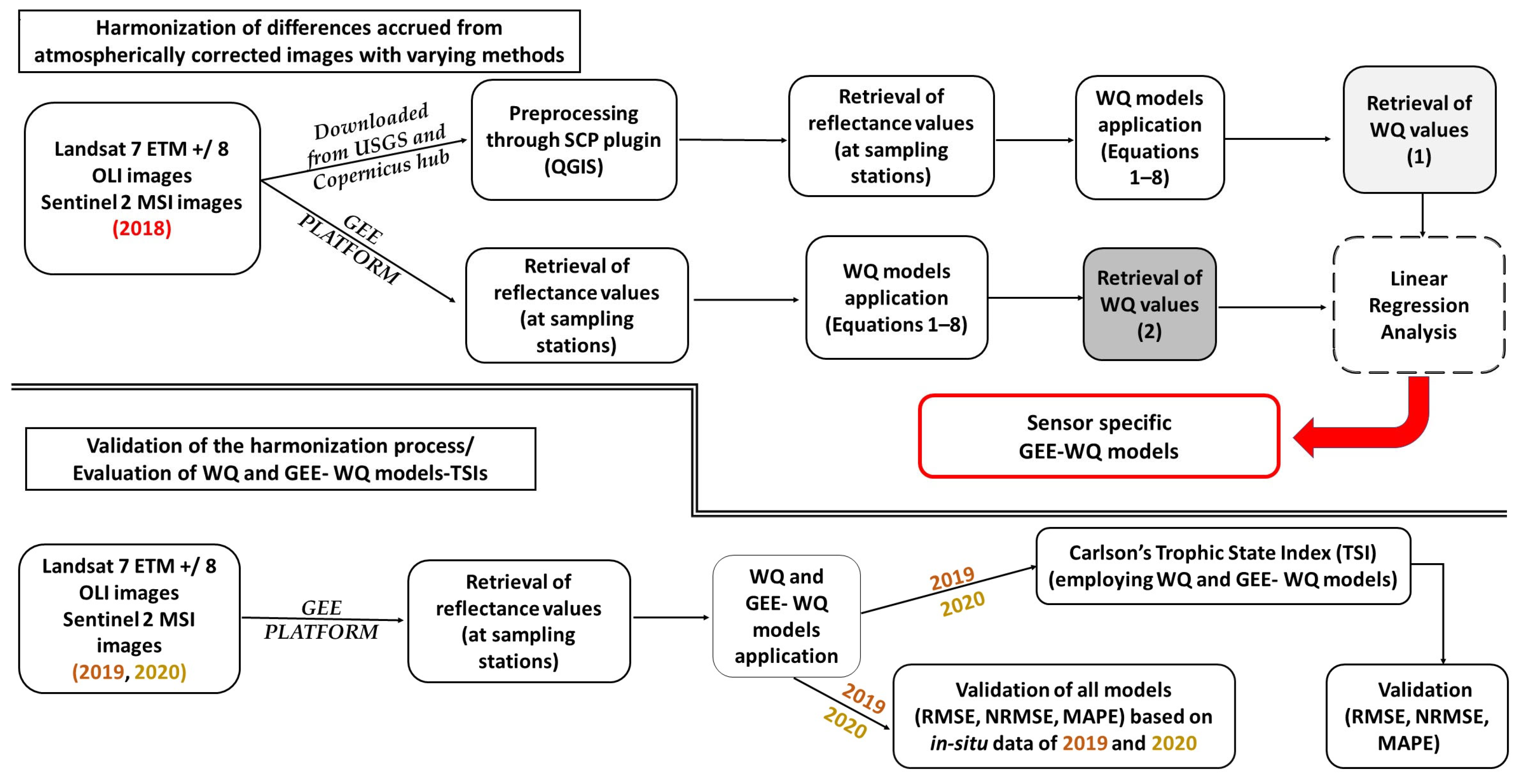
2.3. Harmonization Among SR Products Subjected to Different Atmospheric Correction Methods

In the context of this study, the WQ models developed by [13] for Chl-a and [16] for SDD and TP were initially applied to manually downloaded and DOS1-corrected Landsat 7 ETM +/8 OLI and Sentinel 2 images of 2018 (2 distinctive datasets; Figure 2). Then, the same WQ models employed GEE-derived SR values originating from identical images but undergoing the aforementioned alternative AC methods (Figure 2). Utilized WQ models include the following:
  • Chl-a models (Equation (1): Chl-ageneral—for all lakes-; Equation (2): Chl-anatural—for natural-only lakes-; Equation (3): Chl-aartificial—for artificial-only lakes-);
  • SDD models (Equation (4): Secchigeneral; Equation (5): Secchinatural; Equation (6): Secchiartificial);
  • TP models (Equation (7): TPgeneral; Equation (8): TPnatural).
As far as the spatial and spectral differences among the utilized sensors are concerned, Landsat 7 ETM + and Landsat 8 OLI images have similar spatial resolution (30 m), are statistically comparable and homogeneous over WQ sample sites [29] while both have similar spectral band placements (Supplementary Files, Table S2) for the Blue (ETM + band 1, 0.45–0.52 μm; 8 OLI band 2, 0.45–0.51 μm) and Green bands (ETM + band 2, 0.52–0.60 μm; 8 OLI band 3: 0.53–0.59 μm). Differences are particularly observed in the NIR (ETM + Band 4, 0.76–0.90 μm; 8 OLI Band 5, 0.85–0.88 μm) and to a lesser extent in Red bands (ETM + Band 3, 0.63–0.69 μm; 8 OLI Band 4, 0.64–0.67 μm) [56]. In addition, Sentinel 2 mission carries two satellites, Sentinel 2A and Sentinel 2B. They are both equipped with identical Multispectral Instruments (MSI) capable of acquiring data at 13 bands at different spatial resolutions (between 10 m and 60 m).
Linear regression analyses incorporated WQ values accrued by the employment of (a) manually DOS1 corrected reflectance (dependent variable) and (b) GEE-retrieved reflectance (independent variable) at the same lake sampling stations. This normalization was based on the dataset of 2018 (Figure 2) while the analysis yielded 192 and 210 match-up points of in situ data and integrated Landsat (7 ETM +/8 OLI) and Sentinel 2 images embedded in GEE platform, respectively. Regression analysis included all types of WQ models (Equations (1)–(8)) was conducted separately for Landsat and Sentinel 2 datasets while the spectral bands of each sensor selected and employed in WQ models are presented in Supplementary Files (Table S2).
Chl - a general : log C h l a g e n e r a l = 3.599 0.63 × b l u e r e d 2.183 × ln r e d ln s w i r 2
C h l - a n a t u r a l : log C h l a n a t u r a l = 4.443 1.421 × b l u e g r e e n 3.454 × ln r e d ln s w i r 2 + 1.304 × ( r e d g r e e n )
C h l - a a r t i f i c i a l :   log C h l a a r t i f i c i a l = 2.919 2.011 × ln r e d ln s w i r 1 + 1.449 × r e d g r e e n 1.441 × ln r e d ln b l u e
S e c c h i g e n e r a l : S Q R T S e c c h i g e n e r a l = 1.215 2.479 × b l u e + r e d + r e d b l u e + 3.394 × l n g r e e n l n s w i r 2
S e c c h i n a t u r a l :   S Q R T S e c c h i n a t u r a l = 1.172 1.003 × l o g C h l a ( 1.031 × l o g r e d )
S e c c h i a r t i f i c i a l : S Q R T S e c c h i a r t i f i c i a l = 3.927 1.365 × g r e e n b l u e 0.318 × r e d s w i r 1 0.361 × l o g C h l a
T P g e n e r a l : L o g T P g e n e r a l = 1.425 + 0.452 × l o g C h l a 0.573 × ( l n r e d l n s w i r 1 )
  T P n a t u r a l :   L o g T P n a t u r a l = 0.633 ( 0.704 × l o g S e c c h i ) 0.392 × ( g r e e n r e d )
The regression analysis resulted in the production of the GEE-WQ models while their performance was validated based on the in situ WQ datasets of years 2019 and 2020 (Figure 2). In particular, dataset 2019 yielded 239 pairs of in situ measurements and Landsat 7 ETM +/8 OLI values of reflectance (GEE), accompanied by 242 pairs with Sentinel 2 images while dataset 2020 delivered 220 and 286 paired reflectance of Landsat 7 ETM +/8 OLI and Sentinel 2 (GEE), respectively. The validation of WQ (Equations (1)–(8)) and GEE- WQ models’ performance for years 2019 and 2020 was based on the error metrics Mean Error (ME), Mean Absolute Percentage Error (MAPE), Root Mean Squared Error (RMSE) and Normalized Root Mean Squared Error (NRMSE). MAPE values are expounded according to [57] who created a table (Table 2) containing typical MAPE values and their interpretation concerning the forecasting potential. MAPE’s greatest disadvantage is that the absolute percentage error distribution—characterized by having only positive values with no upper bound—usually has a right or positive skew brought about by the presence of outlier values to this side of the distribution [58]. Hence, if the denominator is extremely small or large, the MAPE value adopts the same behaviour.
In view of the aforementioned limitation of MAPE, NRMSE is used additionally and comparatively; NRMSE (Equation (9)) is an extension of RMSE and is often utilized to compare different datasets or predictive models of different scales (e.g., different units as in our case) and it was calculated by using the range of the true values (difference of minimum and maximum values; Equation (9)). Furthermore, it takes values 0–1. Low values of all error metrics (ME, MAPE, RMSE and NRMSE) indicate the good performance of models.
N R M S E = R M S E Y m a x Y m i n

2.4. Carlson’s Trophic State Index (TSI) and Validation

Based on equations derived from [59], separate TSIs of TP, Chl-a, and SDD were computed while a TSI average was estimated to produce the final trophic state for each lake station. In particular, three types of average TSI were estimated for each station:
  • TSIIN-SITU by employing in situ WQ data;
  • TSIMODELLED by applying WQ models, namely Equations (1)–(8);
  • TSIGEE-MODELLED by applying the hereby-developed GEE-WQ models ().
Then, values of average TSIs were utilized to categorize the lakes according to the trophic status classification system as oligotrophic (TSI value < 30), mesotrophic (TSI value 40–50), eutrophic (TSI value 60–70), and hypereutrophic (TSI value > 70; Table 3). Furthermore, since the scale of the index is arithmetic, it can further describe a larger number of transitional individual trophic state classes (e.g., oligotrophic–mesotrophic, mesotrophic–eutrophic). Classes with No 1, 2, 3, 4, 5 and 6 (Table 3) were assigned to trophic classes Oligotrophic, Oligotrophic–Mesotrophic, Mesotrophic, Mesotrophic–Eutrophic, Eutrophic and Hypereutrophic, respectively, while the frequencies of each dataset (validation years 2019, 2020; TSIMODELLED; TSIGEE-MODELLED) were estimated setting as reference dataset the respective in situ ones (TSIINSITU). Furthermore, the error metrics ME, MAPE, RMSE and NRMSE were likewise utilized for TSIs’ validation.

3. Results

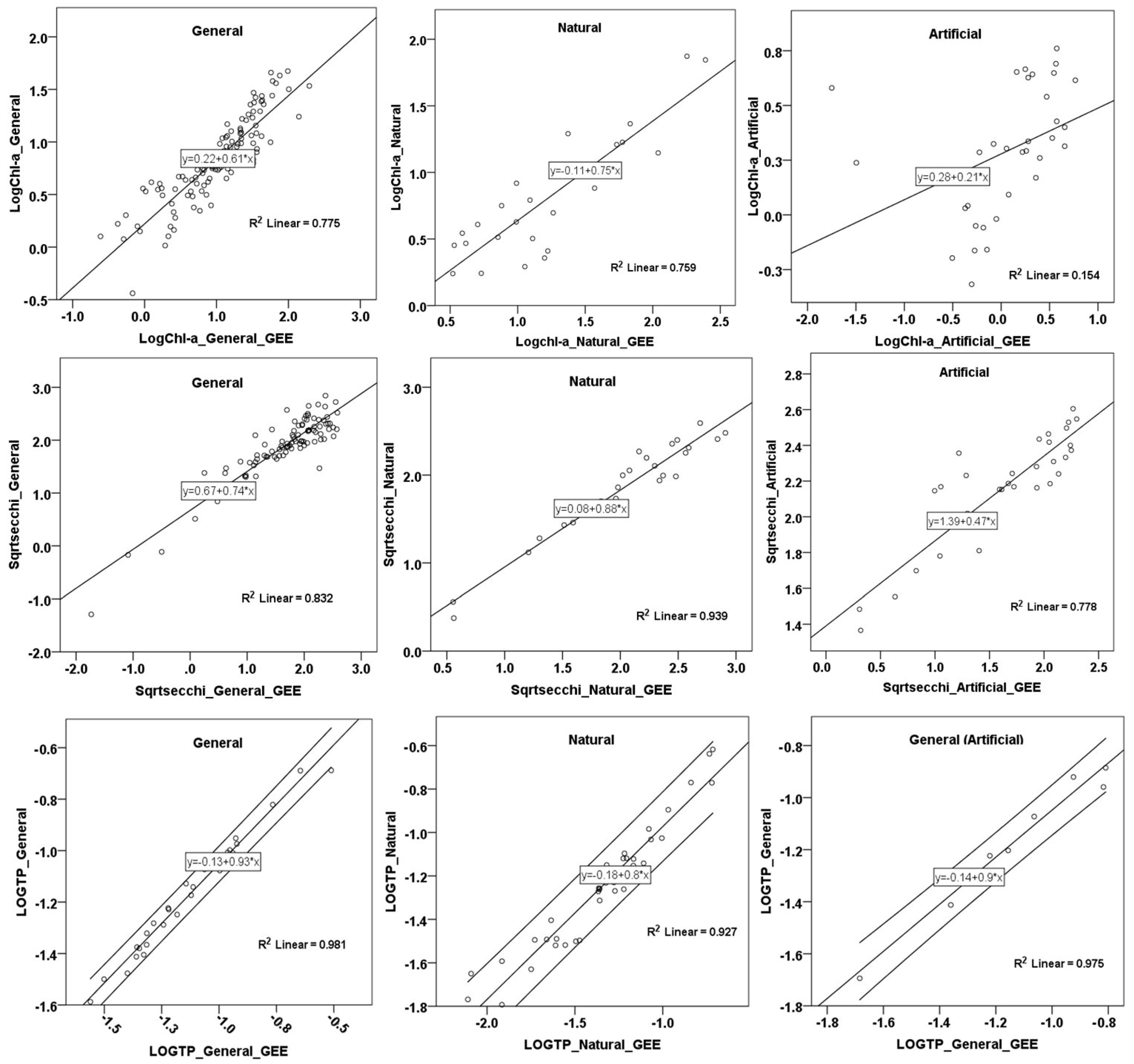
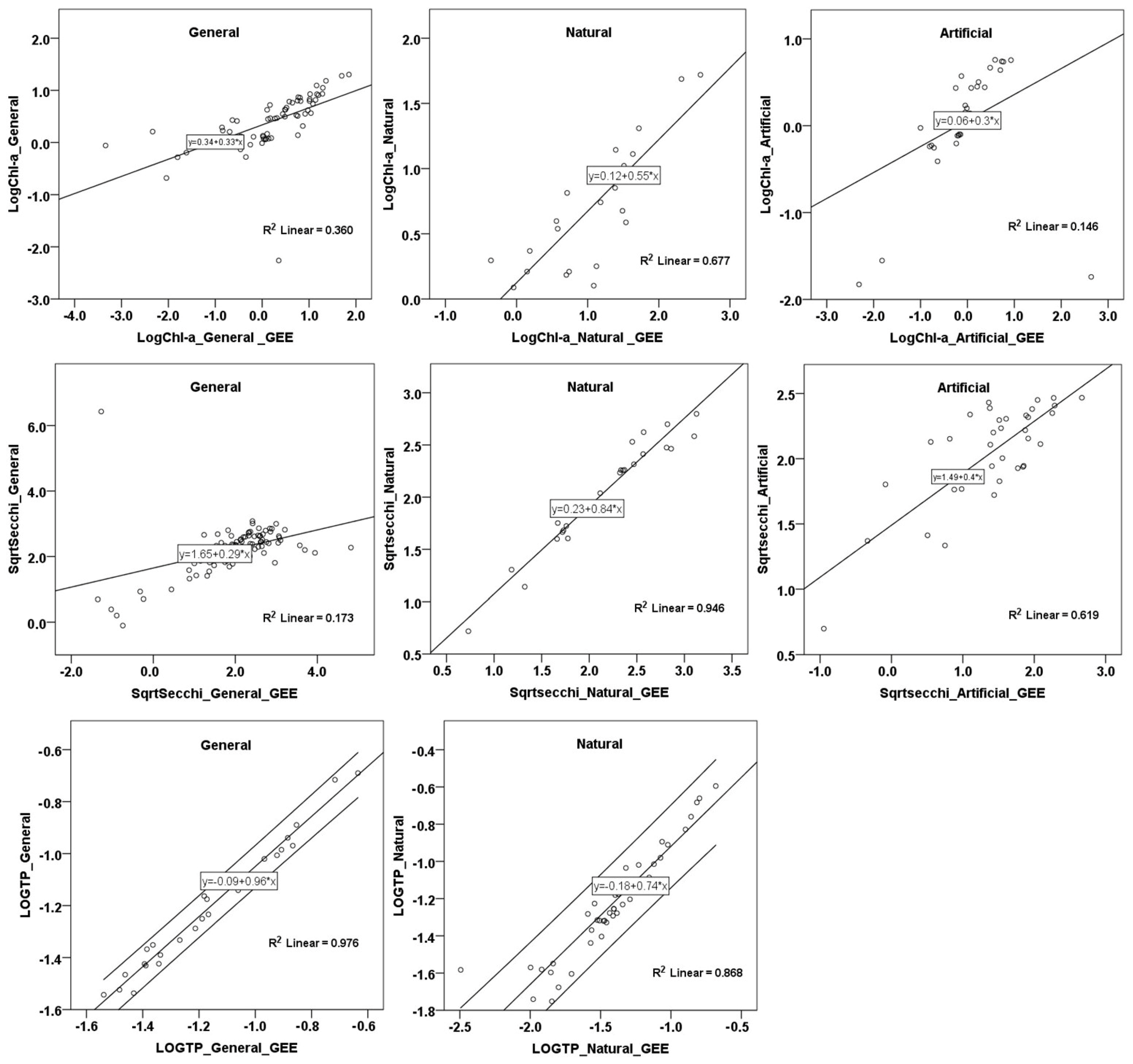
3.1. Harmonization Among SR Values Subjected to Different AC Methods

Linear regression analyses among the double WQ values of 2018 (Chl-a, SDD, TP), concerning both datasets (Landsat 7 ETM +/8 OLI and Sentinel 2), yielded linear equations (GEE-WQ models) accompanied by a high coefficient of determination values (R2; Table 4 and Table 5; Equations (10)–(26); Figure 3 and Figure 4) except for some exceptions.
Based on Table S3 (Supplementary Files), the application of the Chl-ageneral model (Equation (1)) on Landsat images indicated a superiority concerning the ME value when GEE reflectance is used (compared to DOS1 corrected) even though both values of RMSE are similar. On the other hand, the Chl-anatural model (Equation (2)) employing GEE-retrieved data performs worse than the respective DOS1 one, based on values of both ME and RMSE. The Chl-aartificial model (Equation (3)) performs equally well with all AC methods.
Regarding the SDDs, the general model (DOS1; Equation (4)) presents a lower ME value and a similar RMSE to the respective one employing the corrected reflectance retrieved from the GEE platform. The Secchinatural model (Equation (5)), using GEE data, introduces a lower ME value but similar RMSE with the respective one using DOS-1 corrected data. Moreover, the Secchiartificial model (Equation (6)) applied on Landsat images performs better with DOS1-corrected reflectance.
Based on the given statistics, all models predicting total phosphorus by using Landsat images are achieving better results when they employ DOS1-corrected reflectance values. As far as the application of WQ models on Sentinel 2 images is concerned (Table S4 in Supplementary Files), the Chl-a models present a similar pattern to Landsat-based analysis. More particularly, only the Chl-ageneral model (Equation (1)) performs better with GEE-retrieved reflectance whereas natural-only (Equation (2)) and artificial-only (Equation (3)) models are more successful when they employ DOS1 reflectance data. The same behaviour is observed with SDD models, where the general one (Equation (4)) presents better results with the Sen2Cor method (GEE) whereas natural (Equation (5)) and artificial (Equation (6)) ones perform better when employing the DOS1-corrected reflectance. Finally, the performance of the TPgeneral model (Equation (7)) is comparable with both types of corrected reflectance (GEE-Sen2Cor and manually applied DOS1) while the TPnatural model (Equation (8)) delivers better results when exploiting the DOS1 correction method.

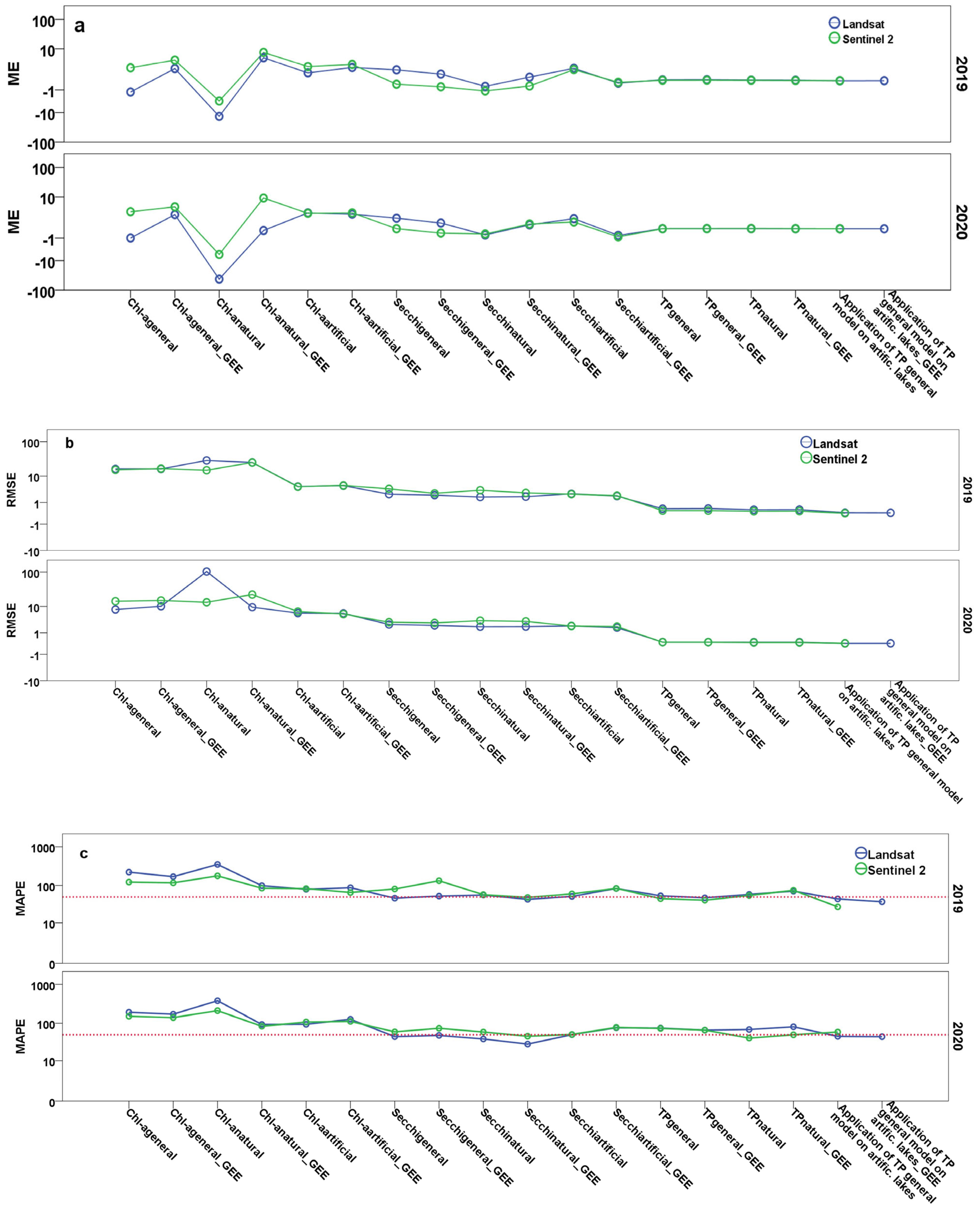
3.2. Validation of Lake WQ Models Employing GEE-Retrieved Reflectance Values

The GEE-WQ models (Table 4 and Table 5; Equations (10)–(26)), derived from the regression analysis of the 2018 dataset, were subsequently validated based on the in situ datasets of 2019 and 2020. Table 6, Table 7 and Table 8 present the evaluation of WQ and GEE-WQ models’ performance, separately for Chl-a, SDD and TP, representing the results of the 2019 dataset for both types of sensors (Landsat and Sentinel 2). The respective data of the 2020 dataset are presented in Supplementary Files (Table S5).

3.2.1. Chl-a Models

Employment of GEE-retrieved reflectance values of Landsat and Sentinel images of 2019 in the Chl-ageneral models (Equation (1)) yielded similar results based on ME and RMSE values while the employment of Sentinel reflectance resulted in lower MAPE values (122.3 vs. 221.7). Considering the corresponding corrected GEE-WQ models (in Table 6 Equations (10) and (19)), the Landsat-employing model resulted in lower ME value (1.5 vs. 3.7 μg/L) and slightly lower RMSE values (16.4 vs. 16.8) compared to the Sentinel-employing model. In general, the application of the GEE WQ models did not contribute to any further enhancement of Chl-a prediction (general model).
Regarding the Chl-anatural models, the initial model employing Sentinel images (Equation (2) in Table 6) performed better compared to Landsat (in Table 6), while the GEE-models (in Table 6 Equations (11) and (20)) improved the Chl-a prediction greatly in natural-only lakes, especially regarding the Landsat-based model and according to ME, RMSE and MAPE values.
The Chl-aartificial model (Table 6; Equation (3)) achieved better results utilizing Landsat reflectance, especially based on ME values, while no improvement was observed concerning the GEE models (in Table 6 Equations (12) and (21)), except for the MAPE values connected to Sentinel reflectance.

3.2.2. SDD Models

The Secchigeneral models (Equation (4); Table 7) performed, in general, better than the Chl-a ones and especially when employing Landsat data compared to Sentinel ones. The SDD GEE model enhanced to a great extent the assessment of SDDs by using Landsat images (in Table 7; Equation (13)) while the respective model employing Sentinel reflectance (in Table 7; Equation (22)) presented only a slight refinement (except for MAPE values in both cases). The Secchinatural models (Equation (5)) performed adequately regarding the prediction of Secchi depths while both the GEE models (Table 7; Equations (14) and (23)) further enhanced their initial performance, especially the Sentinel-employing model. The Secchiartificial models (Equation (6)) performed fairly similarly regarding the sensor used (Table 7) yielding Secchi Depth values with adequate accuracy in relation to in situ ones, while the GEE models (in Table 7; Equations (15) and (24)), further improved the SDD prediction based on ME and RMSE values.

3.2.3. TP Models

The TPgeneral initial model (Equation (7)) performed slightly better with Sentinel images compared to Landsat, while the GEE ones (in Table 8; Equations (16) and (25)) did not manage to improve the TP prediction with the exception of the MAPE values.
The TPnatural model (Equation (8)) employing Sentinel data performed better compared to Landsat (Table 8) while the GEE models (Table 8; Equations (17) and (26)) have not shown any significant differentiation. Application of the TPgeneral model on artificial lakes sampled with 2019 data presented better results when employing Landsat reflectance rather than Sentinel. The GEE-TP model slightly improved the performance of the initial one whereas no GEE-TP model was built for Sentinel data, due to the existence of few records.
The application of all WQ models (including the GEE ones) on the Landsat and Sentinel images of 2020 illustrated similar results to those accrued from the dataset of 2019 (Table S5).

3.2.4. All WQ Models

Based on the values of ME per model and sensor, clustered by year, it can be concluded that the Chl-a models resulted in higher divergences from the in situ values compared to the SDD and the TP models (Figure 5a). Based on negative residual values, it seems that the Chl-ageneral model employing Landsat reflectance overestimates Chl-a concentrations while the same applies for the Chl-anatural models for both sensors but to a greater extent for Landsat. The SDD models have the same behaviour based on the sampling year (except for the GEE Secchinatural model employing Sentinel data) but present differences based on the utilized sensor. Secchigeneral and GEE Secchigeneral models using Landsat data seem to underestimate SDDs whilst respective models employing Sentinel 2 data overestimate those measurements. The TP models in general indicated low residual values (Figure 5a).
The highest RMSE values are also accrued with the application of the Chl-a models, followed by the SDD and the TP models (Figure 5b). The distribution of RMSE values per WQ model is similar between the two years except for the value resulting after applying the Chl-anatural model on Landsat images of 2020. Additionally, Landsat-based Chl-a models suggest higher RMSE values compared to the respective Sentinel ones.
Examining the MAPE values derived from all WQ models and taking into consideration the threshold value of 50 for reasonable forecasting (Table 2 [57]), it can be concluded that most SDD models, followed by the respective TP ones, can be characterized as efficient enough to quantify each corresponding WQ element (Figure 5c). Concerning the application of the Chl-ageneral models (Equation (1)) and the corresponding GEE ones (Equations (10) and (19)), it can be declared that even though there was an enhancement in the models’ performance, the MAPE values are still quite high independently from sensor or year (Figure 5c). The Chl-aartificial models (Equation (3)) do not indicate any improvement concerning the year 2020, but the Sentinel-based model (Equation (21)) applied to the 2019 dataset performs better than the Landsat one (Equation (12); Figure 5c). Even though the Secchigeneral model (Equation (4)) has not been upgraded, the initial uncorrected ones presented highly acceptable MAPE values, indicating a good forecasting performance. In addition to the SDD models, the GEE-Secchinatural models (Equations (14) and (23)) resulted in highly acceptable MAPE values. The GEE-Secchiartificial model (Equation (6)) was not particularly enhanced, but the MAPE values accrued from the initial equations can guarantee a satisfactory SDD quantification.
The GEE-TPgeneral models (Equations (16) and (25)) were improved based on both years and utilized sensors and, particularly, the employment of the 2019 dataset resulted in valuable outcomes (for both sensors). The TPnatural models were also not improved and, concerning the initial models, only those employing the Sentinel 2 reflectance of 2020 are considered reliable to use. As far as the application of the TPgeneral model on artificial lakes is concerned, no safe conclusion can be drawn due to the existence of few available records. Despite this, the Landsat-based models presented an improved performance for both of the studied years. Concerning the NRMSE metric, values range from 0.1 to 1.3, while both of them were observed in 2020 employing Landsat data in the Chl-ageneral and Chl-anatural models, respectively. The average NRMSE values per satellite sensor revealed a light superiority of models employing Landsat compared to Sentinel 2 reflectance (0.21 vs. 0.23) while the utilization of satellite and the in situ dataset of 2019 presented better performance than that of 2020 (0.18 vs. 0.24).

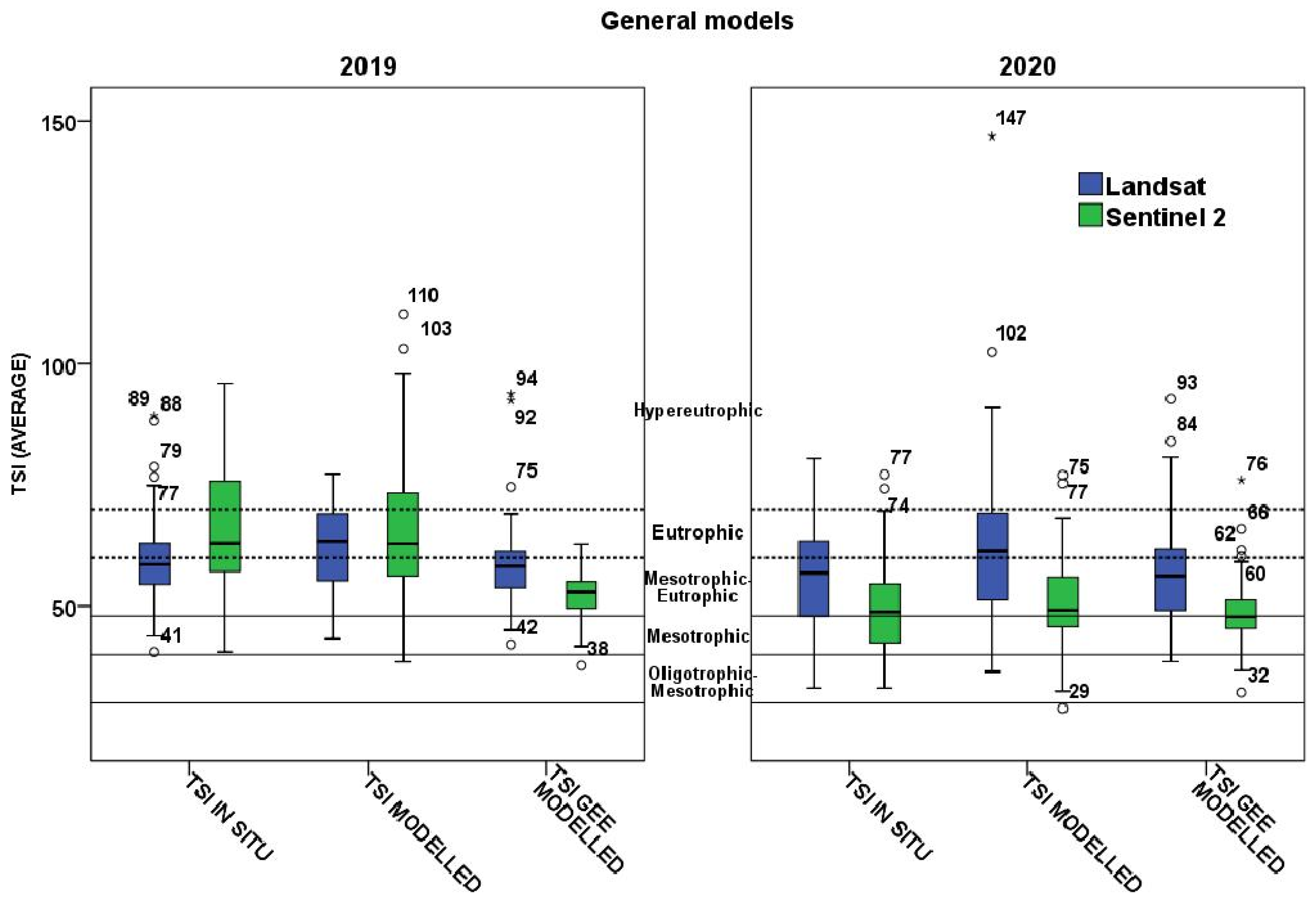
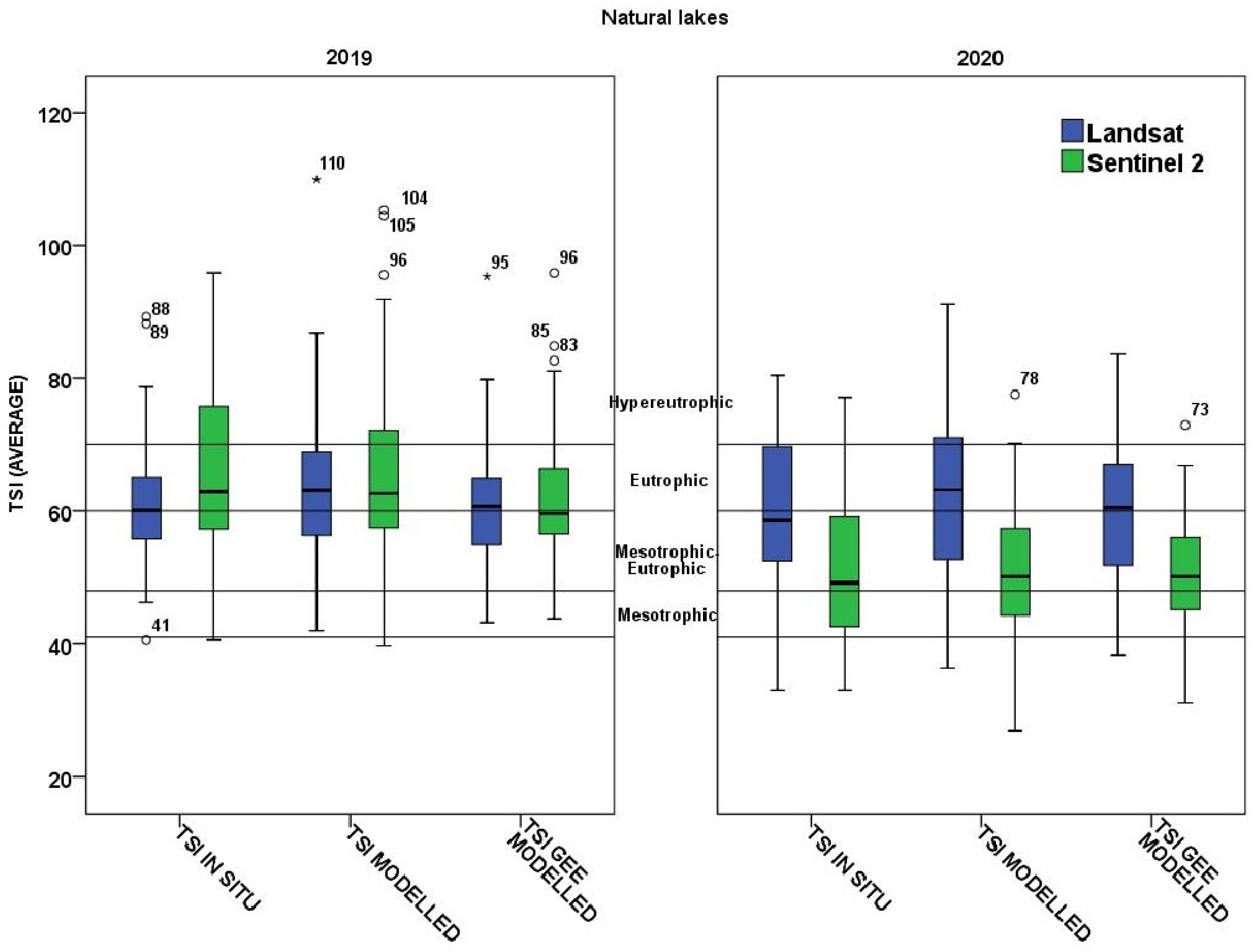
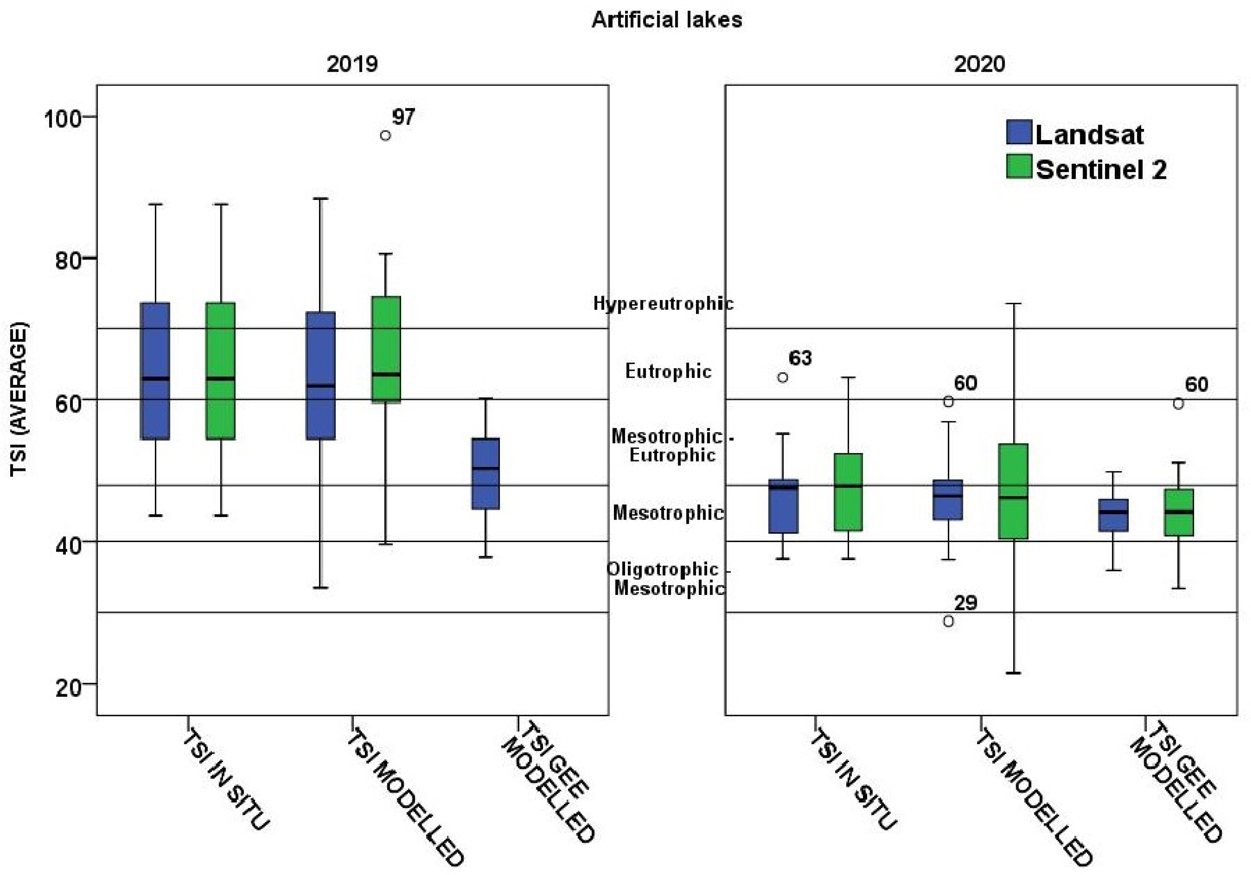
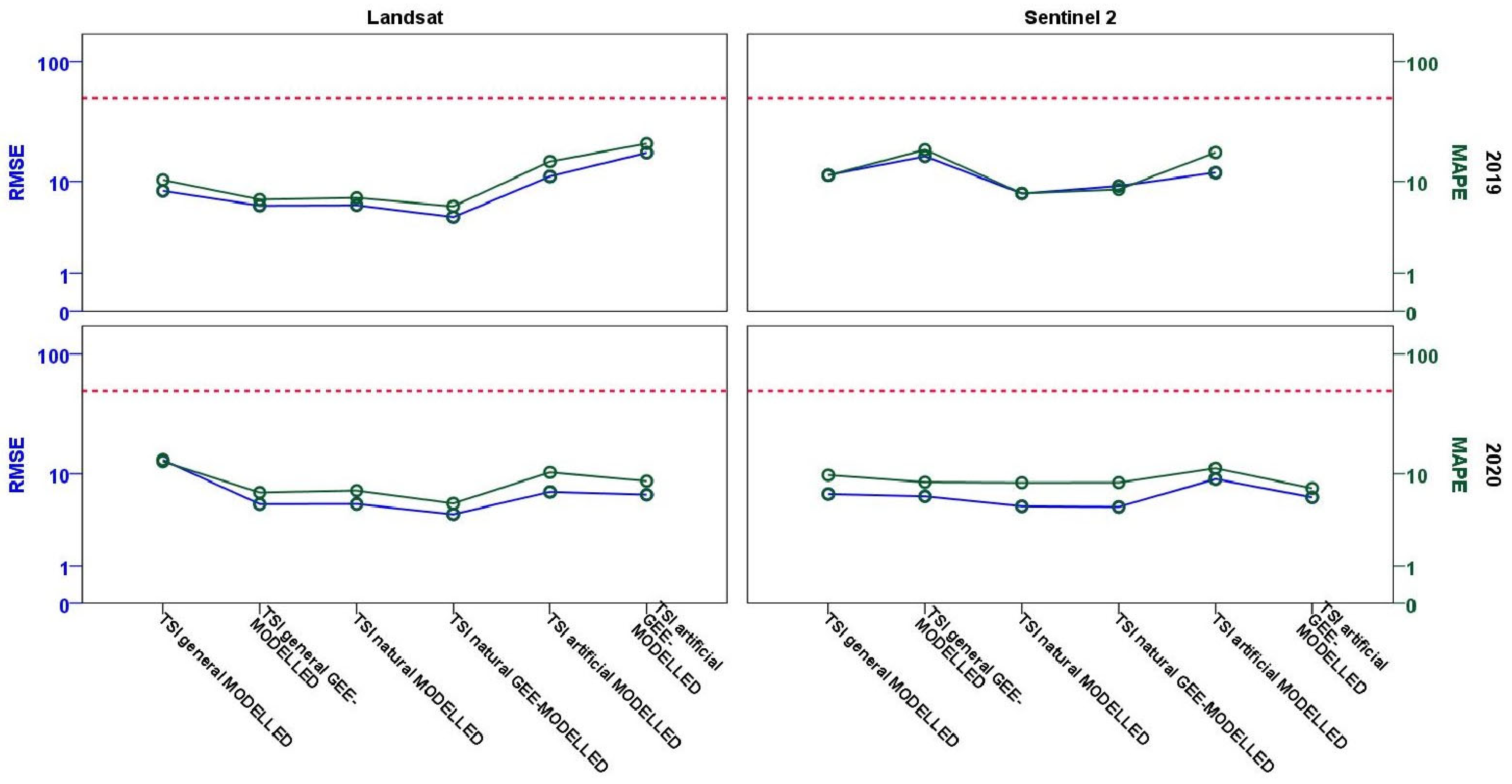
3.3. Satellite-Derived Assessment of Trophic Status of Greek Lakes Based on Carlson’s Trophic State Index (TSI)

In general, the WQ general models (Equations (1), (4) and (7)) employed in trophic status assessment performed satisfactorily concerning all sensors, validation years and the comparison of the TSIMODELLED and the TSIGEE-MODELLED with the respective TSIINSITU (Table 9). As far as the performance of the TSIMODELLED is concerned, the majority of cases are identically classified (class deviation 0) in relation to the TSIINSITU dataset with coincidence percentages equal to 48.8% (Landsat; 2019), 57.8% (Sentinel 2; 2019) and 55.6% (Sentinel 2; 2020). A slightly lower performance was presented by the employment of Landsat images of 2020 in TSIMODELLED, where the majority of cases were misclassified by one class (−1, 46.3%), while the next following class concerns those characterized by total concurrence (41.8%). Furthermore, the rest of the cases misclassified by two classes include only a small number of frequencies, e.g., 3 (out of 41) and 1 (out of 64) cases for Landsat and Sentinel 2 of 2019 and 1 (out of 67) and 4 (out of 45) cases for Landsat and Sentinel 2 of 2020.
Regarding the calculation of TSIGEE-MODELLED, it is observed that even though most of the cases are similarly classified as the respective TSIINSITU (63.4% Landsat of 2019; 62.7% Landsat of 2020 and 51.1% Sentinel 2 of 2020), slightly worse classification was achieved than the TSIMODELLED. In particular, the majority of cases (46.9%) concerning the Sentinel 2 images of 2019 were those misclassified by one class while 16 cases (25%) were misclassified by two classes and one case (1.6%) by three classes of deviation. Furthermore, even though most of the cases (51.1%) of Sentinel 2 data of 2020 presented accurate coincidence with the reference data, three cases (6.6%) were misclassified by two classes.
In terms of the estimation trend per utilized sensor (Figure 6), values of TSIMODELLED tend to be overestimated (e.g., lakes’ WQ is presented as more degraded compared to their actual state) for both validation years when combined with Landsat data whereas when Sentinel 2 data are used, values tend to be equally over- and underestimated in almost similar extents. Concerning the TSIGEE-MODELLED’s values, the estimation trend is clearer with Sentinel 2 data, e.g., TSI values are underestimated to a greater extent (consequently lakes’ WQ is assessed as having better status compared to their real one). On the other hand, Landsat data exhibit a reverse pattern depending on the dataset, e.g., in 2019, most TSIs were underestimated while in 2020 the opposite is the case.
The values of basic statistical error metrics evaluating the general (for all lakes) TSIs’ (TSIMODELLED and TSIGEE-MODELLED) performance are presented in the Supplementary Files (Table S6).
As a whole, trophic status classification of natural lakes (concerning values of both TSIMODELLED and TSIGEE-MODELLED) was particularly successful since most of the cases were identically classified with the respective TSIINSITU ones (Table 10). Concerning the TSIMODELLED, only one case was observed for both the Sentinel 2 data of 2019 (2%) and the Landsat data of 2020 (2%), which was misclassified by two classes of deviation. The immediately following high frequencies concern only one class misclassification (−1, +1). The values of TSIGEE-MODELLED indicate an equally successful trophic status classification compared to TSIMODELLED ones. The majority of cases (TSIGEE-MODELLED) are likewise identically classified as the reference TSIINSITU ones with the misclassified-by-two-classes cases also being observed in the Sentinel 2 data of 2019 (2%) and the Landsat data of 2020 (2%). The estimation trend is clearer regarding the natural lakes (Figure 7). The values of TSIMODELLED are overestimated compared to the in situ ones when Landsat data are utilized whereas the reverse phenomenon is observed with Sentinel data, e.g., the underestimation of TSI values. The exact same pattern is observed concerning the TSIGEE-MODELLED values, which are presented underestimated when combined with Sentinel 2 data for both years whereas Landsat data tend to both over- and underestimate TSIs, but to a greater extent overestimate their values. The values of basic statistical error metrics evaluating the TSIs’ (modelled and GEE-modelled) performance concerning the natural-only lakes are presented in the Supplementary Files (Table S7).
Observing the trophic status classification of artificial lakes, it is concluded that this was less successful than that of natural lakes while the dataset’s size is distinctly smaller (Table 11). Concerning the TSIMODELLED values, it is demonstrated that even though the majority of cases are identically classified to the reference ones, except for the Sentinel 2 data of 2019, there are more cases characterized by a two-class deviation in relation to the natural lakes. In particular, this fact appears in cases concerning the Landsat (23%) and the Sentinel 2 (15.4%) data of 2019, but also both the Landsat (17.7%) and the Sentinel 2 (13.6%) data of 2020. Studying the calculation of TSIGEE-MODELLED values based on the Landsat images of 2019, low performance is indicated, accompanied by 38.5% of cases being misclassified with two, three and four classes of deviation. On the other hand, the TSIGEE-MODELLED values are better when combined with the Landsat images of 2020, where only 5.9% of cases were misclassified by a two-class deviation and the majority of cases (58.8%) were classified similarly to the in situ ones. Equally satisfactory is the performance when combined with the Sentinel 2 images of 2020, where 63.6% of cases were identically classified and only 9.1% of them were characterized by a two-class-from-reference data difference. When studying the TSI values of artificial lakes, no safe conclusion can be made. The TSIMODELLED values tend to be equally over- and underestimated for both years when Landsat data are used (Figure 8). The same pattern is observed with the Sentinel 2 data of 2019 whereas in 2020, the TSI values are clearly underestimated. Regarding the TSIGEE-MODELLED values, all satellite data for both years and sensors tend to underestimate them compared to the respective TSIINSITU ones.The values of basic statistical error metrics evaluating the performance of the TSIs (TSIMODELLED and TSIGEE-MODELLED) of the artificial-only lakes are presented in the Supplementary Files (Table S8).
As far as the distribution of RMSE and MAPE values of TSIgeneral is concerned (Figure 9), it is observed that TSIgeneral MODELLED employing images from 2019 performs better with Landsat data except for the ME value, which is significantly lower (0.69 vs. −2.47) when using Sentinel 2 images. The best performance is also presented with Landsat data for TSIgeneral GEE-MODELLED for both validation years with the only exception of the TSIgeneral MODELLED values of 2020, which are better represented using Sentinel 2 data.
Based on the distribution of RMSE and MAPE values (Figure 9) concerning the natural lakes, the best performance is observed when TSIs are assessed by employing Landsat images either concerning the TSInatural MODELLED or the TSInatural GEE-MODELLED, while this also applies for both validation years (2019 and 2020). However, it should be noted that the assessment of TSInatural utilizing the Sentinel 2 images of 2020 provided a lower ME value (0.67 vs. −3.01).
The values of RMSE and MAPE metrics (Figure 9) regarding the artificial lakes indicated that TSIsartificial MODELLED were more representatively assessed by the Landsat images of both validation years even though the Sentinel 2 data of 2019 provided a significantly lower ME value (−0.95 vs. 2.45). The only exception is the better performance of GEE-modelled TSIsartificial when assessed based on the Sentinel 2 images of 2020 despite the lower ME value (2.79 vs. 3.33) that characterizes the Landsat data.

4. Discussion

This study’s discussion section aims to provide a thorough interpretation of the findings while collating them with those accrued by the relevant international literature. The observed results are also linked to the research objectives providing a better understanding of the methodology’s performance and its significance for lake management.
This study is perhaps the first attempt to facilitate the quantification of spatiotemporal lake WQ across the Greek Lake Monitoring Network of WFD by using multi-sensor reflectance values retrieved from the GEE platform. Landsat (7 ETM +/8 OLI) and Sentinel 2 reflectance values in GEE were matched with concurrent WQ in situ data of 2018 while the same pairs were created with reflectance derived from the respective manually pre-processed images.
The published Landsat-based empirical WQ models of Chl-a [13], SDD and TP [16] were applied twice, employing two (2) different atmospherically corrected reflectance values (DOS1 and other AC methods embedded in GEE) while linear regression analysis among the resulting WQ values, separately for each sensor, yielded WQ-corrected (namely GEE-WQ models) linear equations accompanied by strong associations. Double employment (2018) of differently atmospheric-corrected reflectance values in the WQ models indicated the DOS1 as the most effective method for the quantification of lake WQ elements in almost all cases and for all sensors (Landsat/Sentinel 2); the only exceptions were the Chl-ageneral and Secchinatural models employing Landsat data, where GEE-retrieved reflectance was proved better and the Chl-ageneral and Secchigeneral models employing Sentinel 2 data (Table 12), indicating their better performance (e.g., Sen2Cor compared to DOS1 method).
The results from several studies agree with the superiority of the DOS method regarding the WQ monitoring of inland waters [37,54,55,61]. In particular, ref. [61] studied the extraction of WQ parameters in the King Talal reservoir (Jordan) by testing several AC methods, including DOS, in Landsat 8 and Sentinel 2 images. According to their AC analysis, the DOS algorithm was the most successful in representing the Sentinel 2 satellite image while they recorded that it can be applied to images of both satellite sensors with not much accuracy loss, which was not the case for the rest of the correction techniques examined (dark spectrum fitting -DSF-, atmospheric and topographic correction -ATCOR-, and exponential extrapolation -EXP). Furthermore, ref. [54] compared image-based and physical correction models for retrieving suspended particulate matter (SPM) concentrations in lakes (the United States and Canada) using Landsat imagery. Based on the results, image-based models, particularly the COST (Cosine of the sun zenith angle) and DOS were more appropriate than the physical models for retrieving SPM concentrations in inland waters if the inputs of the physical atmospheric parameters are not well controlled. The basic assumption concerning the physical methods is that they usually use two or more Near-Infrared (NIR) or Short-wave infrared (SWIR) wavebands, whereas the marine signal is assumed to be zero (open ocean waters). However, the signal in the NIR (or SWIR) is not negligible in case 2 waters (inland/coastal), due to the concentrations of particulate matter in inland water bodies, and, consequently, maritime correction over inland water causes low or even negative water reflectance in the visible bands. As a consequence, reflectance over inland water bodies is assessed based on assumptions including zero water-leaving radiance in the NIR (or SWIR) and aerosol origin/type models, resulting in the confusion of this natural optical–physical relationship (in terms of reflectance) of WQ parameters across the electromagnetic spectrum [54].
Additionally, cases of the 2018 dataset that presented low values of coefficient of determination among same-located WQ values concern mainly the Chl-a models (general and artificial) employing Sentinel 2 reflectance. On one hand, it is well known that mapping Chl-a in case 2 waters is a complicated task and characterized by less accuracy since the optical properties are measured based on a compound of dissolved organic matter, dead organic–inorganic particulate matter, and phytoplankton (Chl-a) [13]. On the other hand, the hereby utilized WQ empirical models were developed based on Landsat-7 ETM + and 8 OLI images, which were atmospherically corrected with the DOS1 method; hence, it is expected that not only will it be affected by this factor but also by the corresponding spectral composition and eventually perform better when employing Landsat rather than Sentinel 2 reflectance, as is hereby observed (Table 13). Major exceptions constitute the Chl-anatural, TPgeneral and TPartificial models, which seem to present more reliable results for both validation years using Sentinel 2 images.
Concerning the question of whether the GEE WQ models (corrected) contribute to the improvement of WQ elements’ quantification, the answer is, in general, positive (Table 13). In particular, regarding the Chl-a models, the Chl-anatural model is presented widely enhanced for both satellite sensors and validation years (except for Sentinel 2 in 2020). The SDD models (general, natural, and artificial) illustrated the greatest improvement, compared to the Chl-a and TP models, with the exception of general and artificial-only models employing Sentinel 2 images in 2020. The TP models also provided refined values based on in situ datasets, except for the natural-only ones.
The Chl-ageneral model employing Landsat reflectance yielded an average RMSE of 12.21 μg/L for both validation years, whereas the corresponding value relating to the Sentinel 2 data equals 14.9 μg/L. The GEE-Chl-anatural model is proposed to be utilized in conjunction with Landsat data while the average RMSE value is 17.45 μg/L. The Chl-aartificial MODELLED model presented lower RMSE values, 5.4 and 5.7 μg/L for Landsat and Sentinel 2 reflectance, respectively.
To our knowledge, there are a few recent studies trying to estimate Chl-a concentrations at a large regional scale with GEE. Ref. [62] combined in situ Chl-a data from 1157 lakes (2007) with Landsat data and developed a well-validated lake national model (RMSE = 34.9 μg/L) by using machine learning algorithms built into the GEE. Ref. [29] used GEE to automatically form match-up points from multi-sensor satellite observations with ground WQ samples and then an SVM was developed to map Chl-a concentrations across 12 lakes in the tri-state region of Kentucky, Indiana and Ohio (USA). Furthermore, the RMSE of Chl-a of the SVM model trained by Landsat 8 OLI imagery was 4.42 μg/L. Ref. [35] analyzed four spectral indices—Normalized Difference Vegetation Index (NDVI), Normalized Difference Chlorophyll Index (NDCI), B8AB4, and B3B2—to retrieve Chl-a data for algal bloom identification in two highly dynamic freshwater reservoirs by using Sentinel 2-MSI in GEE. Among the results, NDCI most accurately identified Chl-a across all study sites (highest adjusted R2 = 0.84, lowest RMSE = 0.02 μg/L), followed by NDVI. A few studies have also been conducted on estuarine and marine environments. Ref. [24] extracted Chl-a concentrations of SeaWiFS and Terra/Aqua MODIS embedded in GEE across the Yellow Sea to examine their relationship to green tide while ref. [34] used Sentinel 2 images through the GEE platform to monitor Chl-a concentrations in the Kali Porong Estuary (Indonesia) employing certain estimation formulas. One of the latest studies was conducted by [63] who used Sentinel 2 images and in situ measured data to develop a Chl-a retrieval algorithm based on 13 optical water types (OWTs). The resulting performance was satisfying (R2 = 0.74, RMSE = 0.42 mg/m3, MAE = 0.33 mg/m3, and MAPE = 55.56%) while they then mapped the Chl-a distribution in 3067 of the largest global lakes (≥50 km2) using the GEE.
Except for GEE utilization, other studies of remote estimation of Chl-a concentrations have yielded comparable and, in some cases, slightly higher RMSE values than ours; Ref. [64] presented an RMSE of 18.47 μg/L in the largest artificial reservoir in Córdoba province (Rio Tercero, Argentina) while ref. [55] showed an RMSE of 40 μg/L across certain Spanish lakes and ponds. Additionally, ref. [65] developed an SVM model on Landsat 8 OLI images to estimate the Chl-a concentrations of multiple lakes in China, while they reported an RMSE of 22.64 μg/L.
As far as the SDD models are concerned, all of GEE ones presented enhanced results; Secchigeneral yielded average two-year RMSE values of 2.22 m (Landsat) and 2.7 m (Sentinel 2), Secchinatural model 1.95 m (Landsat) and 2.95 m (Sentinel 2) while the respective RMSE values resulting from the Secchiartificial model were equal to 1.91 m (Landsat) and 2.05 m (Sentinel 2). One of the few studies that combined the derivation of SDD in reservoirs and GEE was conducted by [32] while the resulting RMSE value was particularly low and equals to 32.6 cm. Considering the high difference between this RMSE value and the hereby derived one, it should be noticed that [32] applied a Zsd (Secchi Disk depth) model consisting of a combination of the Normalized Difference Chlorophyll Index (NDCI) and a mechanistic model for the derivation of the absorption coefficient and backscattering. According to [66], those models depict more applicability and reliable results compared to those utilizing the relationship between WQ parameters and in situ measurements. Furthermore, ref. [14] documented the most recent SDD estimation models used in previous studies since 1993, based on RS techniques. Referring to the comparison of their performance, the average RMSE value among those studies is 1.13 m while the highest (1.7 m) was recorded by [67].
Considering the performance of TP models, it is evident that only the TPgeneral model needs the corrected version (GEE) while the model for natural-only lakes stands efficiently without correction. The GEE-TPgeneral model yielded RMSE values of 0.23 mg/L (Landsat) and 0.14 mg/L (Sentinel 2), TPnatural model 0.18 mg/L (Landsat) and 0.11 mg/L (Sentinel 2) while the application of TPgeneral model on artificial lakes—illustrated only in Landsat images—resulted in an RMSE value of 0.02 mg/L. During a thorough literature review, no recent study was detected utilizing GEE for the quantification of TP concentrations in lakes. Nevertheless, a survey was conducted to record RMSE values of remotely sensed phosphorus concentrations to compare with hereby results. Ref. [68] developed a novel semi-analytical algorithm in the eutrophic Lake Taihu, China and the validation showed satisfactory performance (RMSE = 0.01 mg/L). Ref. [69], who also constructed multiple regression equations to retrieve TP concentrations in Nakdong River, Korea, reported a TP regression model accompanied by an RMSE value of 0.01 mg/L. Lastly, ref. [15] established a hybrid model combining genetic algorithms and partial least squares (GA-PLS) to estimate remote TP concentrations in three central Indiana reservoirs and RMSE values ranged from 0.009 to 0.03 mg/L, depending on in situ datasets.
Based on our literature review, only a few studies have examined the trophic status assessment/classification by utilizing the GEE platform, in particular across a large-scale region, due to lakes’ high complexity [3]. Nevertheless, the aforementioned studies mostly utilize Landsat and Sentinel 2 images. One of the latest surveys, conducted by [70], investigated the national freshwater reservoirs of Taiwan. In particular, in situ sampling of 2020 Sentinel 2 satellite data and machine learning classifiers were utilized for effective lake WQ observation across Taiwan. An integrated GEE Python Application Programming Interface (API) pipeline solution was used to overcome labeled data scarcity while the deep neural network (DNN) outperformed the other classifiers, with accuracy comparable to the results obtained by the traditional in situ methods. Nevertheless, despite the lack of GEE-based TSI studies, there are quite a few studies investigating the assessment of lakes’ trophic status based on multiple RS methods. Ref. [3] had a large number of in situ datasets measured from 88 lakes (2804 samples) across China with various optical properties at their disposal. They trained and validated three machine learning methods to model TSI with the optical indicators and derive the determined optical indicator from Landsat images. Based on the results that the total absorption coefficients of optically active constituents at 440 nm perform best in characterizing TSI and that DNN outperforms other models (RMSE = 5.95, MAE = 4.81), they assessed water TSI of 961 lakes (>10 km2) across China. Another study, conducted by [71], focuses on the generation of a 35-year (1986–2020) TSI dataset of 146 lakes in the eastern plain (EP) region in China based on Landsat images while the TSI inversion algorithm was designed for Landsat series after consistency analysis. Furthermore, this RS inversion of the TSI for lakes (>10 km2) was performed for the first time.
Based on the aforementioned and taking into consideration the hereby-developed WQ models’ evaluation, it is proven that the GEE public data are sufficient for mapping Chl-a, SDD, TP concentrations and by extension trophic status in a large geographical region and particularly at a national scale (Greece). Even though the WQ models were developed based on multiple linear regression analyses (MLRs) and Landsat 7 ETM + and 8 OLI images, their efficiency was affirmed when employing GEE reflectance, despite any pre-processing differentiation.

Limitations

During the course of this research, specific factors were identified that may have hindered the achievement of more precise validation results.
Initially, special attention should be given to the integration of different satellite sensors (Landsat 7 ETM +, Landsat 8 OLI and Sentinel 2 MSI). Ref. [50] identified both the potential and the challenges associated with the combined use of Landsat and Sentinel 2 sensors. While they observed a significant correspondence between their spectral bands, discrepancies in recorded radiometric values were also noted. However, the significance of these differences largely depends on the specific application and the approach adopted for multi-sensor time series analysis. On one hand, empirical approaches relying on multispectral indices may be more susceptible to these discrepancies [72]. However, when processing is conducted separately for each image and training is also independent, as in our case, the impact is minimized [45,50]. In addition to this, ref. [50] also documented that the Sentinel 2 MSI Band 8A (vegetation red edge) is the optimal choice from a radiometric perspective when associating Sentinel 2 images with Landsat 8 imagery. Conversely, MSI Band 8 (NIR) is highly recommended for joint use with older Landsat series, such as Landsat 5. However, in this study, the use of Sentinel 2 B08 (NIR) to match with B4 (Landsat 7 ETM +) and B5 (Landsat 8 OLI) may have posed a challenge to achieving more precise and accurate WQ and trophic status validation results when employing Sentinel 2 data.
Another significant limitation factor concerning the integration of Landsat and Sentinel 2 data is the residual impact of water specular reflections. These reflections typically result from variations in the zenith and azimuth angles, as well as differences in the spacecraft altitudes of the respective sensors.
Employment of RS techniques is also restricted by the utilized sensor’s temporal resolution or revisit time. In the context of this research, this feature has surely prevented a more effective validation of lake trophic status monitoring for those cases when the frequency desired was greater than the revisit capacity of Landsat sensors. Another limitation of a similar nature is the dependence on favorable climatic conditions. A significant number of satellite images corresponding to the dates of in situ measurements could not be utilized due to atmospheric interference. This obstacle resulted in the loss of substantial field data, which could have otherwise contributed to a more robust verification of the hereby utilized methodology.
Another factor that may have hindered the extraction of more refined validation results is the uncertainty regarding the precise location of sampling stations. Water sampling in lakes requires careful consideration, as various external factors—including wind, seasonal variations, lake depth, fluctuations in water levels, and accessibility—can lead to positional discrepancies, even when revisiting the same sites. Furthermore, the location of sampling stations plays a crucial role in WQ monitoring, particularly concerning the distinction between land and water and the adjacency effects. In the framework of this study, no prior land/water classification has been conducted, hence there is the possibility that some pixels, while covering land, were defined as water. Nevertheless, since the hereby utilized WQ models were developed by taking this limitation into account, their evaluation is conducted also accompanied by it. Of additional significance is the location of the artificial lakes. One of the primary differences between artificial and natural lakes is that artificial lakes typically exhibit a trophic gradient, transitioning from eutrophic conditions in the upper reaches to oligotrophic conditions near the dam. In particular, reservoirs experience nutrient depletion (particularly phosphorus) due to sedimentation along a downstream gradient, hence in situ data may not accurately reflect the actual conditions of an artificial lake; especially in our case, which concerns the existence of a single station for each studied lake.

5. Conclusions

The estimation of important WQ elements in lakes across Greece by employing reflectance values retrieved from the GEE platform facilitates the monitoring and estimation of their trophic status at a national scale. Therefore, the derived results indicated that WQ models, empirically developed, are applicable to both archived and future Landsat and Sentinel 2 image data despite the different pre-processing methodologies applied. Further, the aforementioned models were trained based on a big dataset collected over different lakes with various optical properties and covering a long enough period of time.
Efficient application of empirical WQ models (and by extension trophic status assessment) employing GEE-retrieved reflectance, exempts users from the complicated AC of raw image products, the key procedure for achieving stable performance. Since one major obstacle to monitoring lake WQ/trophic status is the lack of data for the relevant parameters (Chl-a, SDD, TP) at the relevant temporal and spatial scales, our results confirmed the spatio-temporal stability of the methodology while offering scientists and Greek competent authorities the opportunity to exploit this massive warehouse of data for map long-term WQ trends and identify the underlying possible pollutant threats.

Supplementary Materials

The following supporting information can be downloaded at: https://www.mdpi.com/article/10.3390/rs17111822/s1, Table S1: Summary of descriptive statistics of in situ Chl-a and TP concentrations and Secchi depth values during years 2018–2020; Table S2: Band stack sets and bandwidths (BW) of Landsat 7 ETM +, 8 OLI and Sentinel 2 sensors; Table S3: Error metrics (2018 dataset) of resulted WQ values (Chl-a, SDD and TP) after the employment of both the DOS1 and the GEE retrieved reflectance in WQ models (Equations (1)–(8)) of Landsat images; Table S4: Error metrics (2018 dataset) of resulted WQ values (Chl-a, SDD and TP) after the employment of both the DOS1 and the GEE retrieved reflectance in WQ models (Equations (1)–(8)) of Sentinel 2 images; Table S5: Basic statistical error metrics evaluating the WQ and the GEE-WQ models’ performance in conjunction with in situ WQ dataset of 2020; Table S6: Basic statistical error metrics evaluating the general TSIs’ (modelled and GEE-modelled) performance in conjunction with in situ WQ datasets of 2019 and 2020, applied in both Landsat and Sentinel 2 images. Table S7: Basic statistical error metrics evaluating the natural-only TSIs’ (modelled and GEE-modelled) performance in conjunction with in situ WQ datasets of 2019 and 2020, applied in both Landsat and Sentinel 2 images. Table S8: Basic statistical error metrics evaluating the artificial-only TSIs’ (modelled and GEE-modelled) performance in conjunction with in situ WQ datasets of 2019 and 2020, applied in both Landsat and Sentinel 2 images.

Author Contributions

Conceptualization, V.M.; methodology, V.M., E.D., G.P.P. and D.P.K.; data elaboration, V.M. and R.G.; writing—original draft preparation V.M.; writing—review and editing V.M., G.P.P., E.D. and D.P.K.; supervision, G.P.P., D.P.K. and E.D. All authors have read and agreed to the published version of the manuscript.

Funding

This research received no external funding.

Data Availability Statement

The original contributions presented in this study are included in the article/Supplementary Materials. Further inquiries can be directed to the corresponding author.

Acknowledgments

The authors are thankful for the freely shared in situ data used in this study; data were collected in the framework of the National Water Monitoring Network for lakes, according to the Joint Ministerial Decision 140384/2011, implemented by The Goulandris Natural History Museum, Greek Biotope/Wetland Centre (EKBY). Moreover, this research is part of the PhD dissertation of V. Markogianni at the Department of Natural Resources Development and Agricultural Engineering, Agricultural University of Athens.

Conflicts of Interest

The authors declare no conflicts of interest.

References

  1. Pedreros-Guarda, M.; Abarca-del-Río, R.; Escalona, K.; García, I.; Parra, Ó. A Google Earth Engine Application to Retrieve Long-Term Surface Temperature for Small Lakes. Case: San Pedro Lagoons, Chile. Remote Sens. 2021, 13, 4544. [Google Scholar] [CrossRef]
  2. Fatima, R. Studies on physical, chemical and bacteriological characteristics on quality of spring water in Hajigak iron ore mine, Bamyan province, central Afghanistan. Open J. Geol. 2018, 8, 313–332. [Google Scholar]
  3. Zhang, D.; Shi, K.; Wang, W.; Wang, X.; Zhang, Y.; Qin, B.; Zhu, M.; Dong, B.; Zhang, Y. An optical mechanism-based deep learning approach for deriving water trophic state of China’s lakes from Landsat images. Water Res. 2024, 252, 121181. [Google Scholar] [CrossRef]
  4. Carlson, R.E. A trophic state index for lakes. Limnol. Oceanogr 1977, 22, 361–369. [Google Scholar]
  5. Guan, Q.; Feng, L.; Hou, X.; Schurgers, G.; Zheng, Y.; Tang, J. Eutrophication changes in fifty large lakes on the Yangtze Plain of China derived from MERIS and OLCI observations. Remote Sens. Environ. 2020, 246, 111890. [Google Scholar] [CrossRef]
  6. Walker, W.W. Use of hypolimnetic oxygen depletion rate as a trophic state index for lakes. Water Resour. Res 1979, 15, 1463–1470. [Google Scholar] [CrossRef]
  7. Xu, F.-L.; Tao, S.; Dawson, R.; Li, P.-G.; Cao, J. Lake Ecosystem Health Assessment: Indicators and Methods. Water Res. 2001, 35, 3157–3167. [Google Scholar] [CrossRef]
  8. Zhang, Y.; Zhou, Y.; Shi, K.; Qin, B.; Yao, X.; Zhang, Y. Optical properties and composition changes in chromophoric dissolved organic matter along trophic gradients: Implications for monitoring and assessing lake eutrophication. Water Res. 2018, 131, 255–263. [Google Scholar] [CrossRef]
  9. Li, J.; Wang, S.; Wu, Y.; Zhang, B.; Chen, X.; Zhang, F.; Shen, Q.; Peng, D.; Tian, L. MODIS observations of water color of the largest 10 lakes in China between 2000 and 2012. Int. J. Digit. Earth 2016, 9, 788–805. [Google Scholar] [CrossRef]
  10. Zhang, F.; Zhang, B.; Li, J.; Shen, Q.; Wu, Y.; Wang, G.; Zou, L.; Wang, S. Validation of a synthetic chlorophyll index for remote estimates of chlorophyll-a in a turbid hypereutrophic lake. Int. J. Remote Sens. 2014, 35, 289–305. [Google Scholar] [CrossRef]
  11. Brezonik, P.L.; Olmanson, G.L.; Finlay, J.C.; Bauer, M.E. Factors affecting the measurement of CDOM by remote sensing of optically complex inland waters. Remote Sens. Environ. 2015, 157, 199–215. [Google Scholar] [CrossRef]
  12. Sagan, V.; Peterson, T.K.; Maimaitijiang, M.; Sidike, P.; Sloan, J.; Greeling, A.B.; Samar, M.; Adams, C. Monitoring inland water quality using remote sensing: Potential and limitations of spectral indices, bio-optical simulations, machine learning, and cloud computing. Earth-Sci. Rev. 2020, 205, 103187. [Google Scholar] [CrossRef]
  13. Markogianni, V.; Kalivas, D.; Petropoulos, G.P.; Dimitriou, E. Estimating Chlorophyll-a of Inland Water Bodies in Greece Based on Landsat Data. Remote Sens. 2020, 12, 2087. [Google Scholar] [CrossRef]
  14. Zhang, Y.; Zhang, Y.; Shi, K.; Zhou, Y.; Li, N. Remote sensing estimation of water clarity for various lakes in China. Water Res. 2021, 192, 116844. [Google Scholar] [CrossRef]
  15. Song, K.; Wang, Q.; Liu, G.; Jacinthe, P.-A.; Li, S.; Tao, H.; Du, Y.; Wen, Z.; Wang, X.; Guo, W.; et al. A unified model for high resolution mapping of global lake (>1 ha) clarity using landsat imagery data. Sci. Total Environ. 2022, 810, 15118. [Google Scholar] [CrossRef]
  16. Markogianni, V.; Kalivas, D.; Petropoulos, G.P.; Dimitriou, E. Modelling of Greek Lakes Water Quality Using Earth Observation in the Framework of the Water Framework Directive (WFD). Remote Sens. 2022, 14, 739. [Google Scholar] [CrossRef]
  17. Gholizadeh, M.; Melesse, A.; Reddi, L. A comprehensive review on water quality parameters estimation using remote sensing techniques. Sensors 2016, 16, 1298. [Google Scholar] [CrossRef]
  18. Topp, S.; Pavelsky, T.; Jensen, D.; Simard, M.; Ross, M. Research trends in the use of remote sensing for inland water quality science: Moving towards multidisciplinary applications. Water 2020, 12, 169. [Google Scholar] [CrossRef]
  19. Pizani, F.; Maillard, P. The Determination of Water Quality Parameters by Remote Sensing Technologies: 2000–2020; Universidade Federal de Minas Gerais, [S. l.]: Belo Horizonte, Brazil, 2022; pp. 1–30. [Google Scholar] [CrossRef]
  20. Kumar, L.; Mutanga, O. Google Earth Engine applications since inception: Usage, trends, and potential. Remote Sens. 2018, 10, 1509. [Google Scholar] [CrossRef]
  21. Gomes, V.C.F.; Queiroz, G.R.; Ferreira, K.R. An Overview of Platforms for Big Earth Observation Data Management and Analysis. Remote Sens. 2020, 12, 1253. [Google Scholar] [CrossRef]
  22. Maciel, D.A.; Barbosa, C.C.F.; de Moraes Novo, E.M.L.; Junior, R.F.; Begliomini, F.N. Water clarity in Brazilian water assessed using Sentinel-2 and machine learning methods. ISPRS Int. J. Geoinf. 2021, 182, 134–152. [Google Scholar] [CrossRef]
  23. Zhao, Q.; Yu, L.; Du, Z.; Peng, D.; Hao, P.; Zhang, Y.; Gong, P. An Overview of the Applications of Earth Observation Satellite Data: Impacts and Future Trends. Remote Sens. 2022, 14, 1863. [Google Scholar] [CrossRef]
  24. Li, W.; Yang, Q.; Ma, Y.; Yang, Y.; Song, K.; Zhang, J.; Wen, Z.; Liu, G. Remote Sensing Estimation of Long-Term Total Suspended Matter Concentration from Landsat across Lake Qinghai. Water 2022, 14, 2498. [Google Scholar] [CrossRef]
  25. Gorelick, N.; Hancher, M.; Dixon, M.; Ilyushchenko, S.; Thau, D.; Moore, R. Google Earth Engine: Planetary-scale geospatial analysis for everyone. Remote Sens. Environ. 2017, 202, 18–27. [Google Scholar] [CrossRef]
  26. Jia, T.; Zhang, X.; Dong, R. Long-Term Spatial and Temporal Monitoring of Cyanobacteria Blooms Using MODIS on Google Earth Engine: A Case Study in Taihu Lake. Remote Sens. 2019, 11, 2269. [Google Scholar] [CrossRef]
  27. Zong, J.-M.; Wang, X.-X.; Zhong, Q.-Y.; Xiao, X.-M.; Ma, J.; Zhao, B. Increasing Outbreak of Cyanobacterial Blooms in Large Lakes and Reservoirs under Pressures from Climate Change and Anthropogenic Interferences in the Middle-Lower Yangtze River Basin. Remote Sens. 2019, 11, 1754. [Google Scholar] [CrossRef]
  28. Maeda, E.E.; Lisboa, F.; Kaikkonen, L.; Kallio, K.; Koponen, S.; Brotas, V.; Kuikka, S. Temporal patterns of phytoplankton phenology across high latitude lakes unveiled by long-term time series of satellite data. Remote Sens. Environ. 2019, 221, 609–620. [Google Scholar] [CrossRef]
  29. Wang, L.; Xu, M.; Liu, Y.; Liu, H.; Beck, R.; Reif, M.; Emery, E.; Young, J.; Wu, Q. Mapping Freshwater Chlorophyll-a Concentrations at a Regional Scale Integrating Multi-Sensor Satellite Observations with Google Earth Engine. Remote Sens. 2020, 12, 3278. [Google Scholar] [CrossRef]
  30. Weber, S.J.; Mishra, D.R.; Wilde, S.B.; Kramer, E. Risks for cyanobacterial harmful algal blooms due to land management and climate interactions. Sci. Total Environ. 2020, 703, 134608. [Google Scholar] [CrossRef]
  31. Lobo, F.d.L.; Nagel, G.W.; Maciel, D.A.; de Carvalho, L.A.S.; Martins, V.S.; Barbosa, C.C.F.; Novo, E.M.L.d.M. AlgaeMAp: Algae Bloom Monitoring Application for Inland Waters in Latin America. Remote Sens. 2021, 13, 2874. [Google Scholar] [CrossRef]
  32. Somasundaram, D.; Zhang, F.; Ediriweera, S.; Wang, S.; Yin, Z.; Li, J.; Zhang, B. Patterns, Trends and Drivers of Water Transparency in Sri Lanka Using Landsat 8 Observations and Google Earth Engine. Remote Sens. 2021, 13, 2193. [Google Scholar] [CrossRef]
  33. Bioresita, F.; Hidayatul, U.M.; Wulansari, M.; Putri, N.A. Monitoring seawater quality in the Kali Porong estuary as an area for Lapindo mud disposal leveraging Google Earth Engine. IOP Conference Series: Earth and Environmental Science, Volume 936, Geomatics International Conference 2021 (GEOICON 2021) 27 July 2021, Indonesia (Virtual). IOP Conf. Ser. Earth Environ. Sci. 2021, 936, 012011. [Google Scholar] [CrossRef]
  34. Vaičiūtė, D.; Bučas, M.; Bresciani, M.; Dabulevičienė, T.; Gintauskas, J.; Mėžinė, J.; Tiškus, E.; Umgiesser, G.; Morkūnas, J.; De Santi, F.; et al. Hot moments and hotspots of cyanobacteria hyperblooms in the Curonian Lagoon (SE Baltic Sea) revealed via remote sensing-based retrospective analysis. Sci. Total Environ. 2021, 769, 145053. [Google Scholar] [CrossRef]
  35. Kislik, C.; Dronova, I.; Grantham, T.E.; Kelly, M. Mapping algal bloom dynamics in small reservoirs using Sentinel-2 imagery in Google Earth Engine. Ecol. Indic. 2022, 140, 109041. [Google Scholar] [CrossRef]
  36. Wen, Z.; Wang, Q.; Liu, G.; Jacinthe, P.-A.; Wang, X.; Lyu, L.; Tao, H.; Ma, Y.; Duan, H.; Shang, Y.; et al. Remote sensing of total suspended matter concentration in lakes across China using Landsat images and Google Earth Engine. ISPRS J. Photogramm. Remote Sens. 2022, 187, 61–78. [Google Scholar] [CrossRef]
  37. Nazeer, M.; Nichol, J.E.; Yung, Y.-K. Evaluation of Atmospheric Correction Models and Landsat Surface Reflectance Product in an Urban Coastal Environment. Int. J. Remote Sens. 2014, 35, 6271–6291. [Google Scholar] [CrossRef]
  38. Warren, M.; Simis, S.; Martinez-Vicente, V.; Poser, K.; Bresciani, M.; Alikas, K.; Spyrakos, E.; Giardino, C.; Ansper, A. Assessment of atmospheric correction algorithms for the Sentinel-2A MultiSpectral Imager over coastal and inland waters. Remote Sens. Environ. 2019, 225, 267–289. [Google Scholar] [CrossRef]
  39. Pahlevan, N.; Mangin, A.; Balasubramanian, S.V.; Smith, B.; Alikas, K.; Arai, K.; Barbosa, C.; Bélanger, S.; Binding, C.; Bresciani, M.; et al. ACIX-Aqua: A global assessment of atmospheric correction methods for Landsat-8 and Sentinel-2 over lakes, rivers, and coastal waters. Remote Sens. Environ. 2021, 258, 112366. [Google Scholar] [CrossRef]
  40. Bresciani, M.; Cazzaniga, I.; Austoni, M.; Sforzi, T.; Buzzi, F.; Morabito, G.; Giardino, C. Mapping phytoplankton blooms in deep subalpine lakes from Sentinel-2A and Landsat-8. Hydrobiologia 2018, 824, 197–214. [Google Scholar] [CrossRef]
  41. Markogianni, V.; Kalivas, D.; Petropoulos, G.; Dimitriou, E. An appraisal of the potential of Landsat 8 in estimating chlorophyll-a, ammonium concentrations and other water quality indicators. Remote Sens. 2018, 10, 1018. [Google Scholar] [CrossRef]
  42. Pahlevan, N.; Smith, B.; Schalles, J.; Binding, C.; Cao, Z.; Ma, R.; Alikas, K.; Kangro, K.; Gurlin, D.; Nguyen, H.; et al. Seamless Retrievals of Chlorophyll-A from Sentinel-2 (MSI) and Sentinel-3 (OLCI) in Inland and Coastal Waters: A Machine-learning Approach. Remote Sens. Environ. 2020, 240, 111604. [Google Scholar] [CrossRef]
  43. Bramich, J.; Bolch, C.J.S.; Fischer, A. Improved red-edge chlorophyll-a detection for Sentinel 2. Ecol. Indic. 2021, 120, 106876. [Google Scholar] [CrossRef]
  44. Zhou, Y.; Liu, H.; He, B.; Yang, X.; Feng, Q.; Kutser, T.; Chen, F.; Zhou, X.; Xiao, F.; Kou, J. Secchi Depth estimation for optically-complex waters based on spectral angle mapping—Derived water classification using Sentinel-2 data. Int. J. Remote Sens. 2021, 42, 3123–3145. [Google Scholar] [CrossRef]
  45. Mandanici, E.; Bitelli, G. Multi-image and multi-sensor change detection for long-term monitoring of arid environments with Landsat series. Remote Sens. 2015, 7, 14019–14038. [Google Scholar] [CrossRef]
  46. Tsiaoussi, V.; Kemitzoglou, D.; Mavromati, E. Report on the Application of Phytoplankton Index NMASRP for Reservoirs in Greece; Greek Biotope/Wetland Centre and Special Secretariat for Waters, Ministry of Environment: Thermi, Greece, 2016; 16p. [Google Scholar]
  47. Tsiaoussi, V.; Mavromati, E.; Kemitzoglou, D. Report on the Development of the National Method for the Assessment of the Ecological Status of Natural Lakes in Greece, Using the Biological Quality Element “Phytoplankton”, 1st ed.; Greek Biotope/Wetland Centre and Special Secretariat for Waters, Ministry of Environment: Thermi, Greece, 2017; p. 17. [Google Scholar]
  48. Standard Methods Committee of the American Public Health Association, American Water Works Association, and Water Environment Federation. 4500-p phosphorus. In Standard Methods For the Examination of Water and Wastewater; Lipps, W.C., Baxter, T.E., Braun-Howland, E., Eds.; APHA Press: Washington, DC, USA, 2017. [Google Scholar] [CrossRef]
  49. Mavromati, E.; Kagalou, I.; Kemitzoglou, D.; Apostolakis, A.; Seferlis, M.; Tsiaoussi, V. Relationships among land use patterns, hydromorphological features and physicochemical parameters of surface waters: WFD lake monitoring in Greece. Environ. Process. 2018, 5 (Suppl. S1), 139–151. [Google Scholar] [CrossRef]
  50. Mandanici, E.; Bitelli, G. Preliminary Comparison of Sentinel-2 and Landsat 8 Imagery for a Combined Use. Remote Sens. 2016, 8, 1014. [Google Scholar] [CrossRef]
  51. Ermida, S.L.; Soares, P.; Mantas, V.; Göttsche, F.-M.; Trigo, I.F. Google Earth Engine Open-Source Code for Land Surface Temperature Estimation from the Landsat Series. Remote Sens. 2020, 12, 1471. [Google Scholar] [CrossRef]
  52. Available online: https://documentation.dataspace.copernicus.eu/Data/SentinelMissions/Sentinel2.html (accessed on 10 July 2022).
  53. Chavez, P.S., Jr. An Improved Dark-Object Subtraction Technique for Atmospheric Scattering Correction of Multispectral data. Remote Sens. Environ. 1988, 24, 459–479. [Google Scholar] [CrossRef]
  54. El Alem, A.; Lhissou, R.; Chokmani, K.; Oubennaceur, K. Remote Retrieval of Suspended Particulate Matter in Inland Waters: Image-Based or Physical Atmospheric Correction Models? Water 2021, 13, 2149. [Google Scholar] [CrossRef]
  55. Doña, C.; Sánchez, M.J.; Caselles, V.; Dominguez, J.A.; Camacho, A. Empirical Relationships for Monitoring Water Quality of Lakes and Reservoirs Through Multispectral Images. IEEE J. Sel. Top. Appl. Earth Obs. Remote Sens. 2014, 7, 1632–1641. [Google Scholar] [CrossRef]
  56. Deutsch, E.S.; Alameddine, I.; El-Fadel, M. Monitoring water quality in a hypereutrophic reservoir using Landsat ETM+ and OLI sensors: How transferable are the water quality algorithms? Environ. Monit. Assess. 2018, 190, 141. [Google Scholar] [CrossRef] [PubMed]
  57. Lewis, C.D. Industrial and Business Forecasting Methods; Butterworths: London, UK, 1982. [Google Scholar]
  58. Moreno, J.M.; Pol, A.P.; Abad, A.S.; Blasco, B.C. Using the RMAPE index as a resistant measure of forecast accuracy. Psicothema 2013, 25, 500–506. [Google Scholar] [CrossRef]
  59. Carlson, R.E.; Simpson, J. A coordinator’s guide to volunteer lake monitoring methods. N. Am. Lake Manag. Soc. 1996, 96, 305. [Google Scholar]
  60. Devi Prasad, A.G. Carlson’s Trophic State Index for the assessment of trophic status of two lakes in Mandya district. Adv. Appl. Sci. Res. 2012, 3, 2992–2996. [Google Scholar]
  61. Abdelal, Q.; Assaf, M.N.; Al-Rawabdeh, A.; Arabasi, S.; Rawashdeh, N.A. Assessment of Sentinel-2 and Landsat-8 OLI for Small-Scale Inland Water Quality Modeling and Monitoring Based on Handheld Hyperspectral Ground Truthing. J. Sens. 2022, 2022, 4643924. [Google Scholar] [CrossRef]
  62. Lin, S.; Novitski, L.N.; Qi, J.; Stevenson, R.J. Landsat TM/ETM+ and machine-learning algorithms for limnological studies and algal bloom management of inland lakes. J. Appl. Remote Sens. 2018, 12, 1. [Google Scholar] [CrossRef]
  63. Zhao, D.; Huang, J.; Li, Z.; Yu, G.; Shen, H. Dynamic monitoring and analysis of chlorophyll-a concentrations in global lakes using Sentinel-2 images in Google Earth Engine. Sci. Total Environ. 2024, 912, 169152. [Google Scholar] [CrossRef]
  64. Bonansea, M.; Bazán, R.; Ferrero, S.; Rodríguez, C.; Ledesma, C.; Pinotti, L. Multivariate statistical analysis for estimating surface water quality in reservoirs. Int. J. Hydr. Sci. Technol. 2018, 8, 52–68. [Google Scholar] [CrossRef]
  65. Zhang, T.; Huang, M.; Wang, Z. Estimation of chlorophyll-a Concentration of lakes based on SVM algorithm and Landsat 8 OLI images. Environ. Sci. Pollut. Res. 2020, 27, 14977–14990. [Google Scholar] [CrossRef]
  66. IOCCG. Remote Sensing of Inherent Optical Properties: Fundamentals, Tests of Algorithms, and Applications; Lee, Z., Ed.; Reports of the International Ocean-Colour Coordinating Group, No. 5; IOCCG: Dartmouth, NS, Canada, 2006; ISBN 9781896246567. [Google Scholar]
  67. Allan, M.G.; Hamilton, D.P.; Hicks, B.J.; Brabyn, L. Landsat remote sensing of chlorophyll a concentration in central north island lakes of New Zealand. Int. J. Remote Sens. 2011, 32, 2037–2055. [Google Scholar] [CrossRef]
  68. Zeng, S.; Lei, S.; Li, Y.; Lyu, H.; Dong, X.; Li, J.; Cai, X. Remote monitoring of total dissolved phosphorus in eutrophic Lake Taihu based on a novel algorithm: Implications for contributing factors and lake management. Environ. Pollut. 2022, 296, 118740. [Google Scholar] [CrossRef] [PubMed]
  69. Lim, J.; Choi, M. Assessment of water quality based on Landsat 8 operational land imager associated with human activities in Korea. Environ. Monit. Assess. 2015, 187, 384. [Google Scholar] [CrossRef] [PubMed]
  70. Mukonza, S.S.; Chiang, J.-L. Machine and deep learning-based trophic state classification of national freshwater reservoirs in Taiwan using Sentinel-2 data. Phys. Chem. Earth 2024, 134, 103541. [Google Scholar] [CrossRef]
  71. Hu, M.; Ma, R.; Xiong, J.; Wang, M.; Cao, Z.; Xue, K. Eutrophication state in the Eastern China based on Landsat 35-year observations. Remote Sens. Environ. 2022, 277, 113057. [Google Scholar] [CrossRef]
  72. Van der Werff, H.; Van der Meer, F. Sentinel-2A MSI and Landsat 8 OLI provide data continuity for geological remote sensing. Remote Sens. 2016, 8, 883. [Google Scholar] [CrossRef]
Figure 1. National Lake Monitoring Network in Greece (numbers of sampling stations coincide with the numbers presented in Table 1 in [13]).
Remotesensing 17 01822 g001
Figure 2. Flowchart of research methodology steps (harmonization and validation processes). Different shades of grey color [also distinguished with numbers (1) and (2)] represent the distinctive images whose reflectance are differently atmospherically pre-processed (DOS1-manually and GEE-retrieved) and employed in WQ models. Different years of in situ datasets are highlighted with distinct colors.
Remotesensing 17 01822 g002
Figure 3. Scatter plots between in situ and GEE-estimated WQ parameters of 2018 dataset (for TP lines set at confidence intervals of 95%). On the horizontal axis, the WQ parameters are displayed: Chl-a (first row), Secchi depth (second row), and total phosphorus (third row), while on the vertical axis, the results are shown for the General models (first column), and the models for natural (second column), and for artificial (third column) lakes, while employing reflectance data from Landsat sensors.
Remotesensing 17 01822 g003
Figure 4. Scatter plots between in situ and GEE-estimated WQ parameters of 2018 dataset (for TP lines set at confidence intervals of 95%). On the horizontal axis, the WQ parameters are displayed: Chl-a (first row), Secchi depth (second row), and total phosphorus (third row), while on the vertical axis, the results are shown for the General model (first column), and the models for natural (second column), and for artificial (third column) lakes, while employing reflectance data from Sentinel 2 sensor.
Remotesensing 17 01822 g004
Figure 5. Distribution of (a) ME and (b) RMSE and (c) MAPE values per WQ model clustered by satellite sensor and validation year. (Red reference line to right Y-axis is set to 50, upper threshold value for reasonable forecasting according to [57]).
Remotesensing 17 01822 g005
Figure 6. Box-plots of triple average TSI values (in situ, modelled, GEE-modelled) by employing general WQ models applied in Landsat and Sentinel 2 images of 2019 and 2020, accompanied by their respective trophic status classification. Mild and extreme outliers are marked with a circle and an asterisk, respectively.
Remotesensing 17 01822 g006
Figure 7. Box-plots of triple average TSI values (in situ, modelled, GEE-modelled) by employing natural-only WQ models applied in Landsat and Sentinel 2 images of 2019 and 2020, accompanied by their respective trophic status classification. Mild and extreme outliers are marked with a circle and an asterisk, respectively.
Remotesensing 17 01822 g007
Figure 8. Box-plots of triple average TSI values (in situ, modelled, GEE-modelled) by employing artificial-only WQ models applied in Landsat and Sentinel 2 images of 2019 and 2020, accompanied by their respective trophic status classification. Mild outliers are marked with a circle.
Remotesensing 17 01822 g008
Figure 9. Distribution of RMSE (blue line) and MAPE (green line; right Yaxis) values per type of TSI clustered by satellite sensor and validation year. (Red reference line to right Y-axis is set to 50, upper threshold value for reasonable forecasting; [57]).
Remotesensing 17 01822 g009
Table 1. Main characteristics of the lakes comprising the National Lake Monitoring Network in Greece (WFD) [13,49].
NoNational Name StationSurface (km2)(N)atural/
(A)rtificial
Mean Depth (m)NoNational Name StationSurface (km2)(N)atural/
(A)rtificial
Mean Depth (m)
1Lake Ladona-A-28Lake Petron11.91N3.1
2Lake Pineiou19.64A15.129Lake Zazari2.98N3.95
3Lake Stymfalia-N1.3130Lake Cheimaditida9.82N1.01
4Lake Feneou0.47A10.531Lake Kastorias30.87N3.7
5Lake Kremaston68.43A47.232Lake Sfikias3.96A23.2
6Lake Kastrakiou25.58A33.233Lake Asomaton2.46A20.8
7Lake Stratou7.02A9.634Lake Polyfytou63.49A22.4
8Lake Tavropou21.46A15.035Lake Mikri Prespa A-N3.95
9Lake Lysimacheia10.87N3.536Lake Mikri Prespa B N-
10Lake Ozeros10.57N3.837Lake Megali Prespa A-N17
11Lake Trichonida93.53N29.638Lake Megali Prespa B N-
12Lake Amvrakia13.14N23.439Lake Doirani 133.25N4.6
13Lake Voulkaria7.38N0.9640Lake Doirani 2 N-
14Lake Saltini-N-41Lake Pikrolimni6.30N1.2
15Lake Mornou17.50A38.542Lake Koroneia-N3.8
16Lake Evinou2.68A31.543Lake Volvi70.36N12.3
17Lake Pigon Aoou11.44A20.844Lake Kerkini-A2.19
18Lake Pournariou19.28A29.845Lake Leukogeion0.83A4.05
19Lake Pamvotida21.82N5.346Lake Ismarida-N0.9
20Lake Pournariou II0.56A11.747Lake Platanovrysis2.99A26.4
21Lake Marathona2.17A15.848Lake Thisavrou13.43A38.4
22Lake Dystos-N-49Lake Gratinis0.80A14.2
23Lake Yliki19.96N20.150Lake N. Adrianis-A-
24Lake Paralimni9.96N2.9951Lake Kourna-N15
25Lake Karlas-A0.952Lake Bramianou-A10.1
26Lake Smokovou-A-53Lake Faneromenis0.33A9.98
27Lake Vegoritida47.67N26.52
Table 2. Typical MAPE values and interpretation [57].
MAPEInterpretation
<10Highly accurate forecasting
10–20Good forecasting
20–50Reasonable forecasting
>50Inaccurate forecasting
Table 3. Carlson’s trophic state index values and classification of lakes [4,60].
TSI
Values
Trophic
Status
AttributesNo of Class
<40<30OligotrophicTransparent water1
30–40Oligotrophic–Mesotrophic 2
41–5041–48MesotrophicHigher turbidity, higher algae abundance and macrophytes3
49–50Mesotrophic–Eutrophic 4
51–7051–60Mesotrophic–Eutrophic
61–70EutrophicUsually blue-green algae blooms5
>70HypereutrophicExtreme blue-green algae blooms6
Table 4. Regression analysis basic statistics (2018 dataset) for Landsat images.
EquationsGEE-WQ ModelsNRR2Sensor
(10)LogChl-a_general = 0.221 + 0.61 × (logChl-a_general_GEE)1150.880.78Landsat
(11)LogChl-a_natural = −0.109 + (0.747 × logchl-a_natural_GEE)260.870.76
(12)LogChl-a_artificial = 0.279 + (0.209 × logchl-a_artificial_GEE)330.390.15
(13)SQRTSecchi_general = 0.671 + (0.737 × SQRTSecchi_general_GEE)950.910.83
(14)SQRTSecchi_natural = 0.079 + (0.875 × SQRTSecchi_natural_GEE)260.970.94
(15)SQRTSecchi_artificial = 1.391 + (0.475 × SQRTSecchi_artificial_GEE)330.880.78
(16)LogTP_general = −0.127 + (0.925 × LOGTP_general_GEE)280.990.98
(17)LogTP_natural = −0.177 + (0.796 × LOGTP_natural_GEE)400.960.93
(18)LogTP_artificial = −0.143 + (0.905 × LOGTP_artificial_GEE)110.990.98
Table 5. Regression analysis basic statistics (2018 dataset) for Sentinel 2 images.
EquationsGEE-WQ ModelsNRR2Sensor
(19)LogChl-a_general = 0.338 + (0.329 × logchl-a_general_GEE)640.60.36Sentinel 2
(20)LogChl-a_natural = 0.125 + (0.549 × logchl-a_natural_GEE)230.820.68
(21)LogChl-a_artificial = 0.06 + (0.299 × logchl-a_artificial_GEE)330.380.15
(22)SQRTSecchi_general = 1.646 + (0.291 × SQRTSecchi_general_GEE)1030.420.17
(23)SQRTSecchi_natural = 0.233 + (0.841 × SQRTSecchi_natural_GEE)240.970.95
(24)SQRTSecchi_artificial = 1.490 + (0.399 × SQRTSecchi_artificial_GEE)360.790.62
(25)LogTP_general = −0.086 + (0.963 × LOGTP_general_GEE)270.990.98
(26)LogTP_natural = −0.178s + (0.742 × LOGTP_natural_GEE)420.930.87
No linear regression analysis between TP values (accrued from the application of general model to artificial lakes) derived both from GEE and manual analysis (2018 dataset) due to few records.
Table 6. Basic statistical error metrics evaluating the Chl-a models’ performance in conjunction with in situ WQ datasets of 2019. (The units of ME and RMSE are μg/L, NRMSE has no units while MAPE has percentage units).
EquationModelMERMSENRMSEMAPESensor
(1)Chl-a_general−1.316.40.1221.7Landsat
(10)Chl-a_general_GEE1.516.40.1169.5
(2)Chl-a_natural−13.629.10.2350.5
(11)Chl-a_natural_GEE4.625.40.298.9
(3)Chl-a_artificial0.84.60.279.3
(12)Chl-a_artificial_GEE1.74.90.287.5
(1)Chl-a_general1.715.40.1122.3Sentinel 2
(19)Chl-a_general_GEE3.716.80.1116.8
(2)Chl-a_natural−3.614.90.1177.7
(20)Chl-a_natural_GEE7.425.40.284.9
(3)Chl-a_artificial1.94.50.282.7
(21)Chl-a_artificial_GEE2.44.90.265.5
Table 7. Basic statistical error metrics evaluating the SDD models’ performance in conjunction with in situ WQ datasets of 2019. (The units of ME and RMSE are meters, NRMSE has no units while MAPE has percentage units).
EquationModelMERMSENRMSEMAPESensor
(4)Secchi_general1.272.40.1946.5Landsat
(13)Secchi_general_GEE0.652.20.1752.7
(5)Secchi_natural−0.531.830.1556.2
(14)Secchi_natural_ GEE0.311.90.1643.3
(6)Secchi_artificial1.552.50.351.7
(15)Secchi_artificial_GEE−0.22.010.2483.2
(4)Secchi_general−0.33.80.380.8Sentinel 2
(22)Secchi_general_GEE−0.582.60.2132.7
(5)Secchi_natural−1.163.40.2757.4
(23)Secchi_natural_GEE−0.492.70.2248.7
(6)Secchi_artificial1.312.40.2960.2
(24)Secchi_artificial_GEE−0.132.10.2583.9
Table 8. Basic statistical error metrics evaluating the TP models’ performance in conjunction with in situ WQ datasets of 2019. (The units of ME and RMSE are mg/L, NRMSE has no units while MAPE has percentage units).
EquationModelMERMSENRMSEMAPESensor
(7)TP_general0.070.340.1553.8Landsat
(16)TP_general_GEE0.080.360.1647.5
(8)TP_natural0.050.260.1158.3
(17)TP_natural_GEE0.040.270.1271.1
(7)Application of TP general model on artificial lakes−0.010.040.2144.4
(16)Application of TP general model on artificial lakes_GEE−0.0020.0350.1937.5
(7)TP_general0.030.190.1545.2Sentinel 2
(25)TP_general_GEE0.0390.190.1541.2
(8)TP_natural0.030.140.1254.7
(26)TP_natural_ GEE0.010.150.1274.7
(7)Application of TP general model on artificial lakes0.0020.010.3727.5
Table 9. Frequencies (Freq.) and percentages (%) of class deviations among TSIINSITU and satellite-derived TSIs (TSIMODELLED and TSIGEE-MODELLED) by applying the WQgeneral models (initial and GEE) in satellite images (Landsat, Sentinel 2) of years 2019 and 2020.
Class Deviation Between
General Models
LandsatSentinel 2LandsatSentinel 2LandsatSentinel 2LandsatSentinel 2
TSIINSITU TSIMODELLED
2019
TSIINSITU TSIMODELLED
2020
TSIINSITU TSIGEE-MODELLED 2019TSIINSITU TSIGEE-MODELLED
2020
Freq.%Freq.%Freq.%Freq.%Freq.%Freq.%Freq.%Freq.%
−237.311.611.524.4 24.4
−11434.11218.83146.3817.8614.6 1420.9613.3
02048.83757.82841.82555.62663.41726.64262.72351.1
149.81117.2710.4817.8819.53046.91116.41328.9
2 34.7 24.412.41625.0 12.2
3 11.6
Total4110064100671004510041100641006710045100
Table 10. Frequencies (Freq.) and percentages (%) of class deviations among in situ and satellite-derived TSIs (modelled and GEE- modelled) by applying natural-only models (initial and corrected) in satellite images (Landsat, Sentinel 2) for years 2019 and 2020.
Class Deviation Between
Natural Lakes
LandsatSentinel 2LandsatSentinel 2LandsatSentinel 2LandsatSentinel 2
TSIINSITU TSIMODELLED
2019
TSIINSITU TSIMODELLED
2020
TSIINSITU TSIGEE-MODELLED
2019
TSIINSITU TSIGEE-MODELLED
2020
Freq.%Freq.%Freq.%Freq.%Freq.%Freq.%Freq.%Freq.%
−1926.559.81632.7417.4720.635.9918.4417.4
02264.73466.73163.31252.22161.83160.83571.41252.2
138.81121.612730.4617.61631.448.2730.4
2 1212 1212.0
Total3410051100491002310034100511004910023100
Table 11. Frequencies (Freq.) and percentages (%) of class deviations among in situ and satellite-derived TSIs (modelled and GEE-modelled) by applying artificial-only models (initial and corrected) in satellite images (Landsat, Sentinel 2) from years 2019 and 2020.
Class Deviation
Between
Artificial Lakes
LandsatSentinel 2LandsatSentinel 2Landsat
TSIGEE-MODELLED
2019
LandsatSentinel 2
TSIINSITU TSIMODELLED
2019
TSIINSITU TSIMODELLED
2020
TSIINSITU TSIGEE-MODELLED
2020
Freq.%Freq.%Freq.%Freq.%Freq.%Freq.%Freq.%
−217.7215.415.914.5
−1323.1323.1423.5 317.614.5
0538.5323.1847.11568.2323.11058.81463.6
1215.4538.5211.8418.2538.5317.6522.7
2215.4 211.829.1323.115.929.1
3 17.7
4 17.7
Total13100131001710022100131001710022100
Table 12. Summarized results indicating the best performance of empirical WQ models while employing different AC processors (2018 dataset).
ModelsLandsatSentinel 2
Chl-aGeneralGEEGEE
NaturalDOS1DOS1
ArtificialALLDOS1
Secchi Disk DepthGeneralDOS1GEE
NaturalGEEDOS1
ArtificialDOS1DOS1
TPGeneralDOS1ALL
NaturalDOS1DOS1
ArtificialDOS1DOS1
Table 13. Summarized results indicating the best performance of WQ models among the sensors used (x symbol) when employing GEE-derived reflectance values (2019, 2020) and exploration of the correction necessity via the application of the sensor-specific models (NO* denotes that only reduced MAPE values were observed while YES* denotes increased MAPE values).
2019 Chl-aSecchiTP
ModelsGeneralNaturalArtificialGeneralNaturalArtificialGeneralNaturalArtificial
LandsatX XXXX X
Sentinel 2XX XX
ENHANCEMENT
LandsatNO*YESNOYESYESYES*YESNOYES
Sentinel 2NOYESNO*YESYESYES*YESNONO MODEL
2020 Chl-aSecchiTP
ModelsGeneralNaturalArtificialGeneralNaturalArtificialGeneralNaturalArtificial
LandsatX XXXXX X
Sentinel 2 X XX
ENHANCEMENT
LandsatNOYESNOYES*YESYES*YESNOYES
Sentinel 2NO*NO*NO*NOYESNOYESNONO MODEL
Disclaimer/Publisher’s Note: The statements, opinions and data contained in all publications are solely those of the individual author(s) and contributor(s) and not of MDPI and/or the editor(s). MDPI and/or the editor(s) disclaim responsibility for any injury to people or property resulting from any ideas, methods, instructions or products referred to in the content.

