Integration and Comparative Analysis of Remote Sensing and In Situ Observations of Aerosol Optical Characteristics Beneath Clouds

Abstract

Lidar is the primary tool used to determine the vertical distribution of aerosol optical characteristics. Based on the observation characteristics of the mountain’s gradient, a validation analysis of the remote sensing and in situ observations of the aerosol optical characteristics and research on seasonal, monthly, and daily variations in aerosol optical depth (AOD) were performed using the dual-wavelength Lidar deployed at the foot of Mt. Lu and the aerosol particle-size spectrometer at the top of Mt. Lu. The validation results show that at the comparison heights, under cloudy-sky conditions with strong winds (>3.4 m/s) and high relative humidity (RH) (>70%), the aerosol extinction coefficients between the two sites are in good agreement; thus, the observations at the top of the mountain are more suitable for in situ validation under cloudy-sky conditions; however, the local circulations under clear-sky conditions lead to large differences in the aerosol properties at the same altitude between the two sites and are unsuitable for validation. An analysis of the AOD data from Mt. Lu reveals the following: (1) The AOD seasonal distribution frequencies under both clear-sky and cloudy-sky conditions are unimodal, with a values of 0.2∼0.6, and the inhomogeneity of the aerosol distribution in winter is evident; the seasonal difference in the AOD under clear-sky conditions is more significant, following the order of spring > summer > winter > autumn, and the AOD seasonal difference under cloudy-sky conditions is not obvious. (2) In the analysis of the AOD monthly variations, due to the influence of the meteorological conditions (high humidity, low wind speed) and pollutant transport, the AOD reached its peak in February (clear-sky: 0.63, cloudy-sky: 0.82). (3) Under clear-sky conditions, the negative correlation between the daily variations in AOD, and visibility is more significant during the daytime, and after 12:00, the AOD is positively correlated with $P{M}_{2.5}$; these results indicate that the AOD is affected mainly by pollutants and the boundary layer height. Under cloudy-sky conditions, the peaks in the daytime AOD are related to the morning and evening rush hours, the correlations with the visibility and $P{M}_{2.5}$ are low, and the accumulation of pollutants during the nighttime. And (4) overall, the AOD is greater under cloudy-sky conditions than under clear-sky conditions; this result is likely related to the more favorable subcloud humidity conditions for aerosol hygroscopic growth.

1. Introduction

Atmospheric aerosols are liquid or solid particles suspended in the atmosphere, and are typically between 0.001 and 100 µm in size. These particles are characterized by irregular spatial distributions and small scales of variation, are largely concentrated in the lower atmosphere, and have significant impacts on global climate change, local air quality, and human health [1]. As cloud condensation nuclei, aerosols influence the formation and growth of cloud droplets, altering cloud cover and precipitation [2]. Reducing aerosol emissions may also significantly decrease cloud albedo, which affects the ability of clouds to reflect solar radiation [3]. In addition, aerosols are capable of absorbing and scattering sunlight, modifying atmospheric radiation properties, and further influencing meteorological elements and vertical distribution of pollutants [4]. On foggy, hazy days, aerosols of different particle sizes can carry microorganisms and other harmful substances, potentially threatening to human health [5]. Therefore, aerosol monitoring and analysis are needed to facilitate the assessment of environmental quality and provide a scientific basis for environmental protection [6].

Currently, methods for detecting atmospheric aerosols can be divided into two categories: in situ observation and remote sensing detection. In situ observations, such as aerosol particle size spectrometers and automatic weather stations, enable in situ measurements of the physical or chemical properties of aerosols sampled at a specific location and time [7]. Because in situ observations do not rely on complex atmospheric radiative transfer models to invert aerosol properties, the data collected are generally considered accurate and reliable, and can be used directly for aerosol property analysis. Remote sensing detection methods, such as sun photometers and Lidar, employ noncontact methods to obtain information that is scattered or reflected back from the atmosphere from remote distances [8]. The advantage of remote sensing is the ability to capture aerosol properties with high spatial and temporal resolutions for long-term, continuous observation and retrieval research [9]. Compared with in situ observations, remote sensing detection has a marked advantage in monitoring the spatial and temporal distributions of aerosols for a long time and can capture the characteristics of aerosol distribution on a large scale or in a regional area [10]; however, the data collected via in situ observations are reliable, but limited by the location and the number of observation points and can only provide only point measurements in a local area, causing difficulty in reflecting the overall distribution of the aerosols in a comprehensive way. Therefore, a more detailed comparative study of the remote sensing and in situ observations is important for verifying the reliability of remote sensing data, expanding the spatial range of in situ observations, and supplementing the observational dataset.

In situ observations at the Lower Saxony State Agency for Ecology in Hanover, Germany, with ceilometer (CT25K) near-range backscatter data and particulate sensors at 43 m above, revealed a high correlation between the $P{M}_{10}/P{M}_{2.5}$ concentrations in the relatively clean regions of the atmosphere [11]. On clear days without the influence of long-range dust transport, a close correlation between the in situ $P{M}_1$ concentrations measured by an aerosol chemical speciation monitor located at 260 m above the ground in the Beijing Meteorological Tower and the carrier-to-noise ratio of the Lidar was also observed [12]. However, constrained by the spatial limitations of the meteorological towers, middle and large monitoring equipment cannot be deployed, and conducting comparative observations at higher altitudes becomes difficult. Although airplane observations can provide data in the vertical direction at high altitudes, they cannot achieve continuous and stable observations [13]. Owing to the large spatial scale and high requirements on the location of equipment deployed, approximate in situ observations of remote sensing detection above 1 km have not yet been reported in the relevant literature.

Lidar is an active remote sensing method that receives and analyzes signals reflected or scattered back from an emitted laser beam to obtain information about the observed target [8]. With the development of laser technology, Lidar has been able to conduct vertical detection with high temporal and spatial resolutions from ground or satellite platforms, has also developed from single-wavelength single-function to multiwavelength multifunctionality, and has attained unattended and automated operation [14]. After decades of development, Lidar has become an important tool for atmospheric aerosol detection and research, providing abundant data resources for the development of related research [15]. When Lidar detects aerosols under cloudy-sky conditions, the laser has difficulty penetrating the clouds because of attenuation. Here, the effective detection height of Lidar is lower than the tropopause [16]. For example, scholars have reported that when clouds are above 6 km, the ratio of the distance-corrected signal to the backward scattering of the atmospheric molecules is at its minimum in the vertical range of 3∼5 km of Lidar detection, and the altitude in this range can be selected as the calibration height [17]. When detecting low clouds, to avoid the influence of the clouds on the Lidar signals, researchers have used the near-end calibration method. Liu et al. demonstrated that if the near-end calibration value could be accurately calculated, the Fernald forward integral is reliable for retrieving the aerosol backscatter coefficients, and they further proposed setting the laser transmitter port as the starting place and using an iterative method to determine the ranges of extinction coefficients at the calibrated heights and calculated the aerosol extinction coefficient profile under the clouds [18,19]. Zhong et al. directly set the calibration height at 5 m, and calculated the boundary value based on the visibility meter at the same height [20].

On the basis of the ground-based Mie-scattering Lidar (acronym: Lidar) deployed at the foot of Mt. Lu, in this study, adaptive wavelet threshold denoising is used on the Lidar signals, and the visibility data are combined with this denoising to retrieve aerosol extinction coefficients beneath the clouds over the Meteorological Bureau of Lushan city. The fusion analysis of the remote sensing data for aerosol optical characteristics and the in situ observations via an aerosol particle size spectrometer are carried out to explore the background meteorological features above 1 km, and are suitable for in situ comparative observations. Furthermore, in this study, the characteristics and differences in the seasonal, monthly, and daily variations in the AOD at Mt. Lu under clear-sky and cloudy-sky conditions are discussed.

2. Measurement Sites, Instrumentation and Data

2.1. Overview of the Observation Regions and Data

Mt. Lu is located in the northern of Jiangxi Province, China, and the mountain is oriented northeast–southwest with most peaks over 1 km in elevation, and is surrounded by plains and small hills [21]. The Lushan Meteorological Bureau is located in Guling town of Mt. Lu, and the altitude difference from the Lushan city Meteorological Bureau at the foot of Mt. Lu is approximately 1128 m. During the period of January 2023 to February 2024, a continuous observation experiment of aerosol optical characteristics was carried out at Mt. Lu, and the locations of the observation sites are shown in Figure 1; the instrumentation and data used in this study are listed in

Table 1. Overview of observation equipment information.

Observation Site	Location	Equipment/Data Source	Data	Resolution
Lushan City Meteorological Bureau	29.44°N, 116.04°E; 37 m (elevation)	Lidar	532 nm echo data; Visibility data Cloud base	5 min (2 min for 10–18 January 2024 only); 7.5 m 5 min
		Laser Ceilometer Dual Polarization Ka-band Continuous Wave Cloud Radar Automatic Weather Station	Reflectivity data	5 s; 10 m
			Relative humidity; 10 m wind	10 min
Lushan Meteorological Bureau	29.56°N, 115.98°E; 1168 m (elevation)	Welas	Aerosol number concentration 2m temperature; Relative humidity; 10 m wind speed and direction	10 s
		Automatic Weather Station		hourly
Jiujiang Comprehensive Industrial Park Monitoring Station of China National Environmental Monitoring Centre	29.60°N, 115.91°E, 79 m (elevation)	https://www.cnemc.cn/sssj (accessed on 9 June 2024)	$P{M}_{2.5}$ mass concentration	hourly
Others	26°N∼34°N, 110°E ∼ 120°E	https://cds.climate.copernicus.eu/ (accessed on 9 June 2024)	ERA-5 reanalysis data	0.25° × 0.25°
	29.3°N∼29.9°N, 115.7°E∼116.2°E	https://gmao.gsfc.nasa.gov/reanalysis/MERRA-2/ (accessed on 9 June 2024)	MERRA-2 reanalysis data (AOD, 550 nm)	0.5° × 0.625°; monthly

.

ERA-5 is a high-resolution reanalysis dataset released by the European Centre for Medium-Range Weather Forecasts, which is generated via data assimilation and numerical prediction models, and has the characteristics of high spatial and temporal resolution, high accuracy, and high reliability [22]. The Modern-Era Retrospective analysis for Research and Applications, Version 2 (MERRA-2) dataset, which is released by NASA’s Office of Global Modeling and Assimilation, contains a variety of product data, including the AOD data. In its assimilation system, MERRA-2 accounts for a variety of satellite and ground-based AOD data, such as MODIS, MIRS and AERONET, to provide more reliable and stable AOD data [23].

During the observation period of 2023, a total of 323 days of valid Lidar data were attained, and their monthly distributions are shown in Figure 2. All data are given in local standard time (LST = UTC + 8).

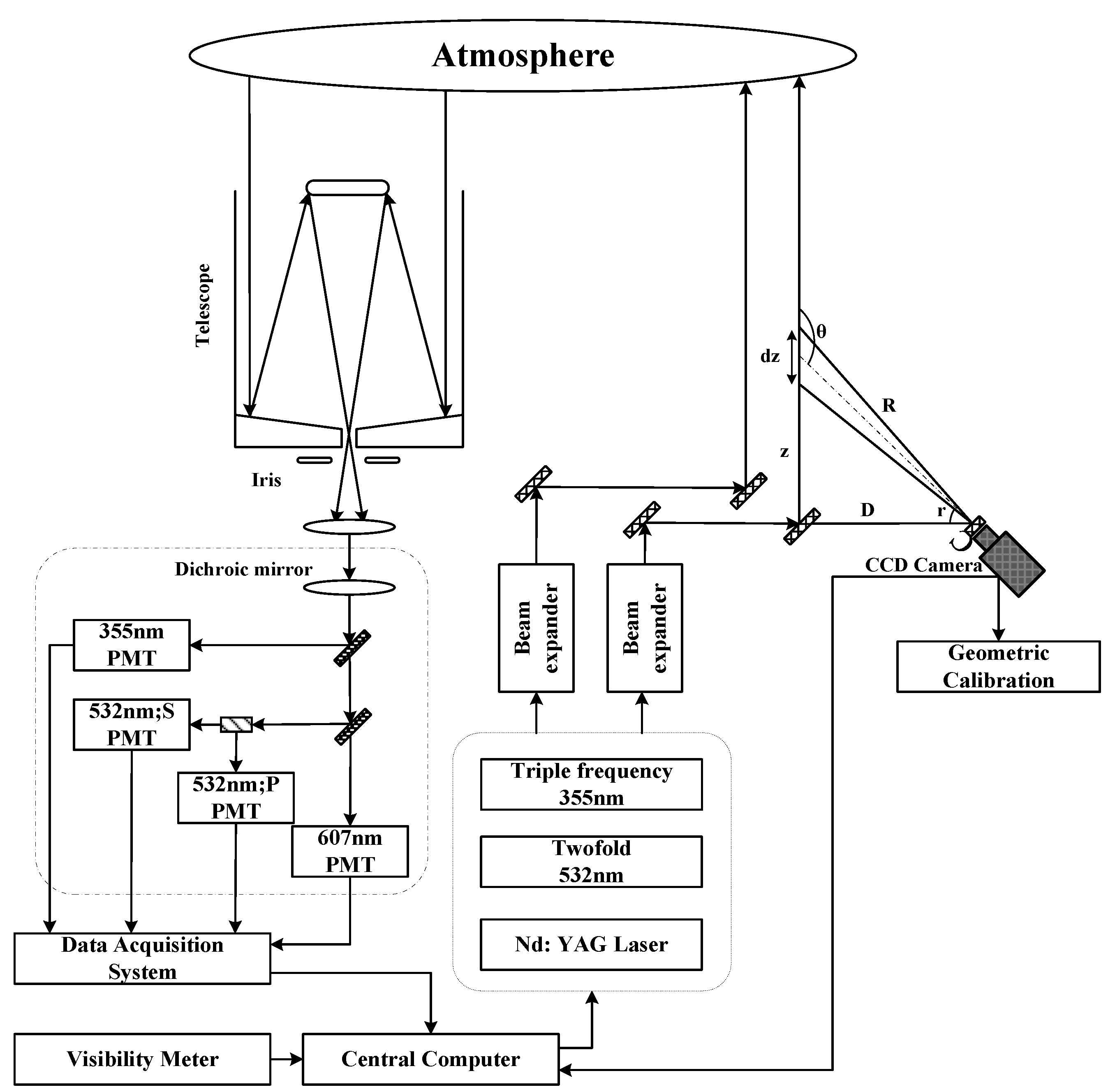
2.2. Main Instrumentation

The Lidar system (Hefei Zhongke Guangbo Quantum Technology Co., Ltd, Hefei, China) is composed of a emission unit, a receiving unit, and a control unit; its emission wavelengths are 355 nm and 532 nm and the detection schematic is shown in Figure 3. The system uses the second and third frequency outputs of the Nd:YAG laser as the emission sources. The pulsed laser is directed vertically into the atmosphere after the beam expander and light guide, and a telescope with an effective receiving aperture of 400 mm is used to receive the backscattered signals. The signals received by the telescope are beam split by the grating and then directed into photomultiplier tubes (PMTs) in the corresponding channels, and the optical signals are converted into electrical signals [24]. Furthermore, the Lidar system is equipped with a visibility meter and two charge-coupled device (CCD) cameras. The visibility meter is placed on the top of the Lidar square pod, about 3.8 m above the ground (Figure S1), and the CCD cameras are used to correct the geometric factors of the near-surface transition region of Mie-scattering Lidar to overcome the blind zone of traditional backscattering Lidar and provide strong support for complementary near-surface atmospheric aerosol data [25].

Table 2. Main parameters of the Lidar detection.

Modules	Parameters	Values
Lidar	Wavelength	355 nm, 532 nm
	Frequency	20 Hz
	Time interval	2 min, adjustable
	Spatial resolution	7.5 m
Visibility Meter	Measurement range	6 m–80 km
	Accuracy	±10%
	Light source	Infrared LED
CCD Camera	Measurement range	20 m–1.5 km
	Wavelength	532 nm
	Pixel count	4652 × 3522

lists the primary detection parameters of the Lidar system.

Welas is an aerosol particle size spectrometer produced by PALAS, Germany, and is used for direct measurements of near-surface aerosols. The main parameters are listed in

Table 3. Main parameters of Welas.

Parameters	Values
Analyzed flow	5 L/min
Measurement range	0.1–10 µm
Concentration limit	10,000 pcs/cm3
Time interval	10 s

. The Welas spectrometer consists of two main parts: a controller and a particle sensor. The controller is designed to control the entire operation of the system, including starting the vacuum pump to collect the air samples with the aerosol particles into the sampling chamber. In the sampling chamber, the air samples flow at a stable speed, and the particle measurement sensor is based on the principle of light scattering and measures the intensity and angular distribution of the scattered light from the air samples; thus, the aerosol particle size distribution and number concentration can be accurately measured [26].

2.3. Data Processing

For the signals received by Lidar, signal decoding, background denoising, geometric factor correction, and distance correction are needed before the aerosol coefficients are retrieved. Moreover, during detection, the Lidar signals inevitably suffer multiple types of noise interference from both the internal system and the external environment [27]; thus, the distance-corrected signals need to be further smoothed and denoised. In this study, considering the nonstationary characteristics of the Lidar signals [28], and that their frequency components may change during different time periods [29], the wavelet threshold denoising method with the determined number of decomposition layers is used (Method S1).

Ground-based Lidar achieves precise detection of aerosol vertical profiles by measuring the scattering signal of the laser beam during propagation [30]. When the Lidar system is in vertical observation mode for the emission of the laser beams into the atmosphere, the elastic backscattered power received at different heights by the telescope can be expressed based on the fundamental Lidar equations [31]:

$$\begin{array}{cc}\hfill P(z)& =EC\beta (z)T(z)/z^2\hfill \end{array}$$

(1)

where E is the output monitoring pulse, C is the system calibration constant, and $\beta (z)$ and $T(z)$ are the backscattering cross sections and atmospheric transmittance at height z, respectively. In this study, based on the Fernald method, atmospheric molecules and aerosols are considered separately in order to retrieve the aerosol extinction coefficients. The Lidar ratio of atmospheric molecules satisfies $S_m=8\pi /3$, and the backscattering and extinction coefficients (${\beta }_m(z)$, ${\alpha }_m(z)$) of atmospheric molecules in the vertical direction can be calculated based on the U.S. Standard Atmospheric Model of 1976 [32]. The aerosol Lidar ratio is assumed to be 50 sr. Under clear-sky conditions, Lidar has a wide detection range, and aerosol extinction coefficients can be retrieved via remote calibration and the Fernald backward integration method. Under cloudy-sky conditions, the laser might be unable to penetrate thicker clouds, and the detection height is limited; thus, the traditional remote calibrated method might involve certain errors [33]. According to the Bouguer–Lambert law, the total extinction contribution of aerosols and atmospheric molecules can be calculated using visibility data. Therefore, it the aerosol extinction coefficient profiles in the effective detection range are able to be retrieved by applying the near-end calibration method coupled with visibility. Equation (2) is the Fernald forward integration equation,

$$\begin{array}{cc}\hfill X& =exp[-2(S_a/S_m-1){\int }_{z_c}^z{\alpha }_m(z)dz]\hfill \end{array}$$

(2)

$$\begin{array}{cc}\hfill {\alpha }_a(z)& ={\displaystyle \frac{X{P}_L(z,{\lambda }_L)z^2}{\frac{P_L(z_c,{\lambda }_L)z_c^2)}{(S_a/S_m){\alpha }_m(z_c)+{\alpha }_a(z_c)}-2{\int }_{z_c}^{z}X{P}_L(z,{\lambda }_L)z^{2}dz}}-S_a/S_m{\alpha }_m(z)\hfill \end{array}$$

(3)

After analysis, the visibility at 45 m of Lidar retrieved can better fit the visibility meter better (Method S2); thus, 45 m near the ground is set as the calibrated height, and the calibrated parameters are calculated according to Equations (3) and (4) [34].

$$\begin{array}{cc}\hfill \alpha & =(3.912/V){(\lambda /0.55)}^{-q}\hfill \end{array}$$

(4)

$$\begin{array}{cc}\hfill q& =\left\{\begin{array}{cc}0.585V^{1⁄3},\hfill & V\le 6\mathrm{km}\hfill \\ 1.3,\hfill & 6<V<50\mathrm{km}\hfill \\ 1.6,\hfill & V\ge 50\mathrm{km}\hfill \end{array}\right.\hfill \end{array}$$

(5)

In this research, the signals from the superimposed parallel and vertical channels of Lidar at 532 nm are used for aerosol extinction coefficient retrieval, which can be expressed as Equation (5), with P and S denoting the parallel and perpendicular channel signals, respectively, and k is the gain coefficient of polarization channel,

$$\begin{array}{cc}\hfill Signal& =P+S\times k\hfill \end{array}$$

(6)

Based on the aerosol particle information (particle radius and number concentration) detected by the Welas, retrieval of the aerosol extinction coefficients was via the meter scattering theory [35]. Considering the altitude difference between the Lidar and Welas results, the Lidar signal at 1125 m was selected for the in situ comparison observations. In general, setting the temporal resolution to 30 min is not suitable for the dynamic comparative assessment of in situ particles [11]; under weak atmospheric turbulence and a relative humidity below 80%, 5 min means of the Doppler beam swinging wind Lidar and the tower-based particulate matter carrier-to-noise ratios were highly correlated (R² = 0.93) [12]. Therefore, to offset the difference in the horizontal distance, a 10 min mean of Lidar and Welas data were used. To ensure that the data bands were consistent, the AOD at 532 nm for Lidar was interpolated to obtain an AOD of 550 nm [36].

3. Results

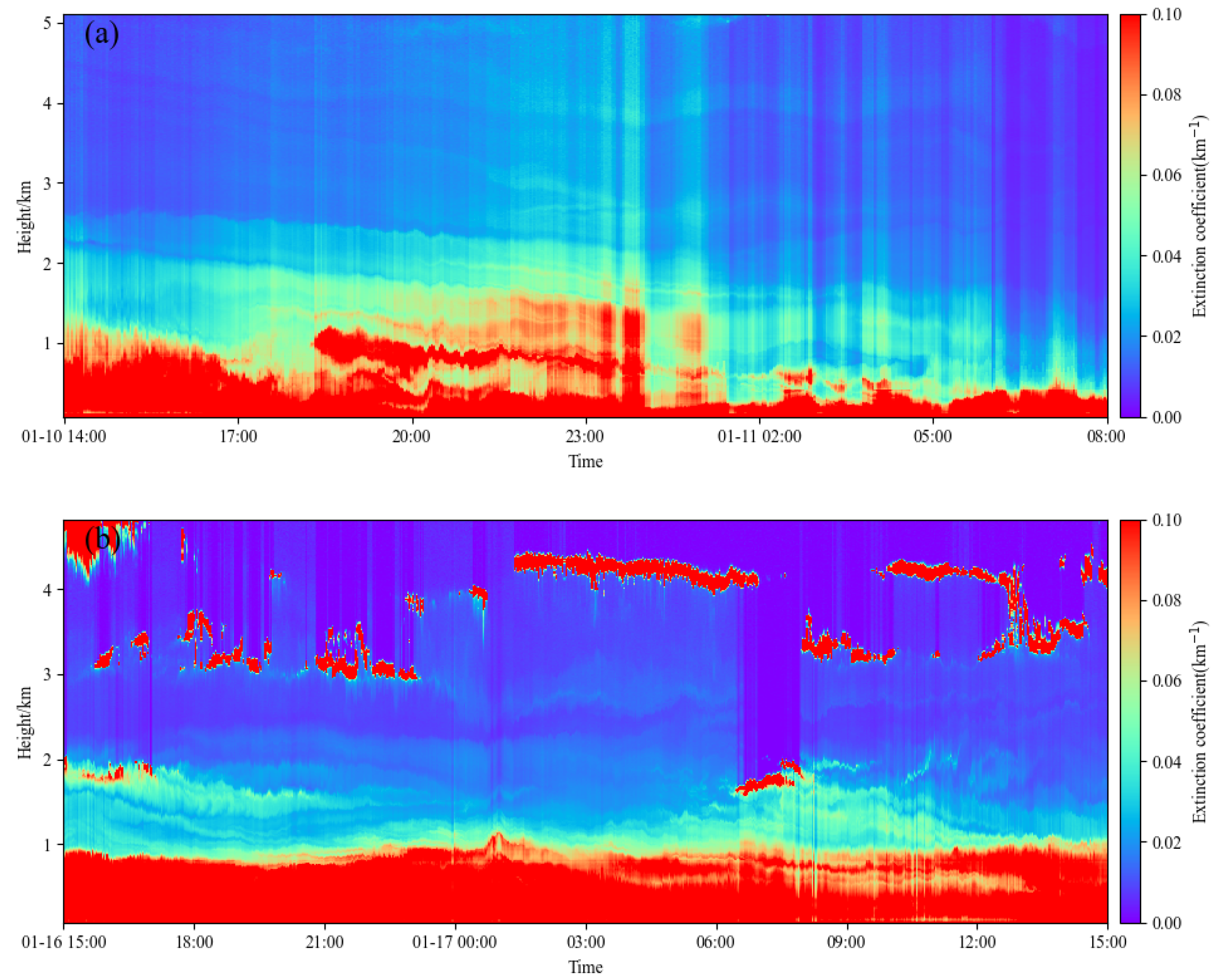
3.1. Comparison of the Lidar and 1125 M Welas Aerosol Extinction Coefficients Measurements

In January 2024, we used the Lidar and Welas to conduct a 10-day (9–19 January 2024) short-term observational experiment. To ensure data quality, we excluded data affected by precipitation (due to attenuation of the Lidar signals by rainfall), low clouds (the cloud bases below the altitude of the Welas location), and power outages. On this basis, we selected relatively continuous periods of 4 days for comparative analyses. Figure 4 shows the temporal and spatial aerosol extinction coefficients detected by Lidar during the observation period. In Figure 4a, the aerosols were mainly distributed within 2 km near the ground, and at 18:30 on 10 January, an aerosol layer of about 200 m thick appeared at about 1 km near the ground, and gradually became thinner, with large fluctuations appearing in the early morning of 11 January, which then gradually dissipated. Compared with the previous day, the aerosol extinction system on the 11 January was relatively low, and the extinction coefficients at the 1 km height were mainly between 0.02 and 0.05 (km⁻¹). In Figure 4b, the high aerosol extinction coefficient area is mainly concentrated below 1 km, the cloud layer was located within 3∼5 km, and some aerosol particles were distributed beneath clouds. Particularly, on the 17th, there was a cloud layer at a low altitude of about 2 km from 6:00 to 8:00, the aerosol extinction coefficient beneath clouds showed a more obvious increase, and remained high for a period of time after the cloud layer was dissipated. The Ka-band cloud radar and ceilometer also observed the clear-sky and cloudy-sky on 10 January and 17 January, respectively (Figure 5). During the observation period, only those from 15:00 on 16 January to 15:00 on 17 January experienced cloudy-sky conditions. Under cloudy-sky conditions, the lowest height of the clouds was approximately 1.57 km; this value was greater than where Welas was located. Thus, the comparative analysis between the Lidar and Welas data were based on the extinction coefficients of the aerosols beneath the clouds. Overall, the correlations of the two instruments (Phase I and Phase II) obviously differed (Figure 6); here, the extinction coefficients of the Lidar and Welas in Phase I greatly differed with time, whereas those in Phase II are more similar.

During Phase I (under clear-sky conditions), the first great difference between the Lidar and Welas data occurred from 18:00 on 10 January to 02:00 on 11 January. During this period, the 10 m wind direction of the Lushan Meteorological Bureau was north, with the wind speed and relative humidity decreasing. The wind speed reached a minimum of 0.3 m/s, and the humidity varied approximately 10%. When the temperature remained below 5 °C, the extinction coefficient of Welas decreased, whereas the extinction coefficient of Lidar increased. After 04:00 on 11 January, the wind shifted to the southwest, and the temperature and wind speed tended to be stable, but the relative humidity increased. At this time, the extinction coefficients of Welas increased, whereas the extinction coefficients of Lidar began to decrease and fluctuated. According to the corresponding moment of the ERA-5 data collection, at 20:00 on 10 January, Mt. Lu was situated in the southern extension of the bottom of a high-pressure region, with 850 hPa influenced by northward airflow (Figure 7a); on 11 January, Mt. Lu was situated north of the high pressure region, with 850 hPa influenced by northwesterly airflow (Figure 7b). Under the continuous control of high surface pressure, the downward airflow at 850 hPa was beneficial for developing a dry and clear atmosphere. During Phase I, the wind direction at the top of Mt. Lu was different from the 850 hPa horizontal wind field, and the characteristics of the mountain valley breeze circulation of Mt. Lu was the major reason for the large difference in aerosol extinction coefficients in the comparison of these in situ observations [37].

In Phase II (under cloudy-sky conditions), the Lidar and Welas extinction coefficient trends were relatively consistent. According to meteorological observations, southerly winds were the dominant wind during this period, with the wind speed and relative humidity greatly increased compared with those in Phase I. At 22:00 on 16 January and 00:00 on 17 January, the wind speed reached a maximum of 5.7 m/s, the humidity remained above 75%, and the temperature slightly varied at 8 °C. At 20:00 on 16 January and 08:00 on 17 January, Mt. Lu was situated in or on the edge of the high-humidity area (RH > 60%), with winds at 850 hPa > 10.8 m/s, and was mainly influenced by the southwesterly flow. The warm and humid air was transported from low to high latitudes, and water vapor was abundant at 1500 m (Figure 7c,d).

Based on the hourly meteorological observations at the Lushan Meteorological Bureau during the observation period, the effects of relative humidity and wind speed variations on the horizontal aerosol distribution were analyzed. According to Figure 8a, under dry environmental conditions (RH < 40%), the aerosol extinction coefficients retrieved via Lidar tended to be greater than those retrieved via Welas, and the two datasets displayed a weak correlation (R = 0.24). As the relative humidity increased, the degree of aggregation of the data increased. However, at most times, the aerosol extinction coefficients calculated via Welas were slightly higher than those calculated via Lidar. In high-humidity environments (RH > 70%), the data clustered strongly around the median line and had a high correlation (R = 0.91).

The data were classified according to the Beaufort scale (level 1: 0.3–1.6 m/s, level 2: 1.6–3.4 m/s, level 3 and above: >3.4 m/s). As shown in Figure 8b, under weak wind conditions (level 1∼2), the extinction coefficient distributions of the two instruments were relatively dispersed with a weak correlation, but when the wind speed (WS) increased to level 3 and above, both datasets had a high correlation (R = 0.85); these results indicated that in the non-static atmosphere, the local circulation characteristics were not evident in the mountainous areas [38], aerosols mixed horizontally were relatively homogeneous at the same height at both locations, and at this time, the mountain-top was suitable for in situ observations of the extinction coefficients beneath the clouds.

In order to explain the comparative validation of the remote sensing in situ observation of aerosol optical characteristics carried out, we present a schematic diagram of this observation (Figure 9).The aerosol particle size spectrometer located at the top of Mt. Lu carries out direct in situ observation, while Lidar deployed at the foot of the mountain is used in remote sensing observation, and the two pieces of equipment have a vertical distance of about 1.1 km and a horizontal distance of about 14.5 km. Under cloudy-sky conditions (the clouds are above Mt. Lu), when the wind speed exceeds 3.4 m/s and the relative humidity over 70%, the aerosol extinction coefficients measured by Lidar at 1.1 km are closer to the values detected by Welas, and at this time, the aerosols at the two locations at 1.1 km achieve a more adequate mixing in the horizontal direction.

3.2. Characteristics of the AOD Variation on Mt. Lu

3.2.1. Seasonal Variation in AOD

The validation of the AOD retrieved by Lidar based on the monthly mean AOD data of MERRA-2 in 2023 (Figure 10) reveals a good match of AOD at 550 nm between Lidar and MERRA-2 (Pearson = 0.93, RMSE = 0.05); the Lidar data can be used to analyze the AOD variation characteristics at Mt. Lu under both clear-sky and cloudy-sky conditions.

According to Mt. Lu’s climatic features, the seasons can be grouped into winter (December, January, February), spring (March, April, May), summer (June, July, August), and autumn (September, October, November) [39]. The AOD of detected Lidar is the vertical integral of the extinction coefficient of aerosols within the entire effective detection height; for the cloudy-sky conditions, only the aerosols are detected beneath clouds. Although aerosols are mainly concentrated beneath clouds, aerosol particles are also present above clouds and are brought by vertical transport or long-range transport. Therefore, undetected aerosols above clouds can lead to an underestimation of the AOD. In 2023, Mt. Lu’s frequency distributions of AODs under clear-sky and cloudy-sky conditions for the different seasons are shown in Figure 11. Generally, the AOD distributions for the different seasons under clear-sky and cloudy-sky conditions are unimodal and are mainly concentrated between 0.2 and 0.6 (clear-sky conditions: 76.49% in spring, 86.7% in summer, 89.11% in autumn, and 88.96% in winter; cloudy weather: 71.95% in spring, 76.66% in summer, 79.30% in autumn, 75.66% in winter); here, the standard deviation (SD) of the AOD is greater in winter (

Table 4. Mean and standard deviation of seasonal variation in AOD.

Season	Clear-Sky		Cloudy-Sky
	Mean	SD	Mean	SD
Spring	0.54	0.06	0.58	0.11
Summer	0.45	0.07	0.52	0.05
Autumn	0.39	0.04	0.50	0.03
Winter	0.44	0.16	0.55	0.24

), and the inhomogeneity of the aerosol distribution is more significant.

Under clear-sky conditions (Figure 11a), AOD is small, shows evident differences between the seasons, and is more likely to be affected by the seasonal wind direction and humidity. The distribution of the mean AOD values is as follows: spring > summer > winter > autumn (Table 4), and the summer and winter AODs are similar. This trend is consistent with the seasonal trend of AOD at the Jinsha background station, and this station is located in the humid subtropical monsoon climatic zone [40]. The AOD is large in spring and winter (with a relatively large distribution in large-value zones), and these results are similar to those from other scholars who applied the RIEMS-Chem model to simulate the seasonal mean values of AOD under clear-sky conditions in the middle and lower reaches of the Yangtze River; the daytime AOD is located in large-value zones in spring and winter [41]. Polluted air masses from the North China Plain and the Yangtze River Delta region are transported to Jiujiang in the direction of Chizhou and Anqing during spring and winter [42]; moreover, dusty weather is high in spring, and dust aerosols transported by dust storms in the north can lead to an increase in AOD throughout eastern China [43]. Summer (MEANAOD = 0.45, Table 4) is more affected by humidity, and the plentiful precipitation resources of Mt. Lu are conducive to the diffusion and wet deposition of the aerosol particles [44]. Moreover, the water surface area of Poyang Lake reaches a maximum in summer, which can provide more water vapor resources. The Mt. Lu area is successively affected by the quasi-stationary fronts and Meiyu fronts in South China during spring and summer, and the amount of water vapor in the air significantly increases. Aerosol particles are also more likely to experience hygroscopic growth under the influence of the East Asian monsoon [45]. In autumn, cold air from the north moves southward, and Mt. Lu is dominated by dry and cold northerly winds [46], and lower relative humidity and good horizontal transport conditions are beneficial to aerosol diffusion and transport, leading to a lower AOD in autumn.

The AOD under cloudy-sky conditions is greater than that under clear-sky conditions (with a greater distribution in the large-value zones), but the monthly mean differences in AOD are not significant during the four seasons. Although the seasonal variation in AOD is also affected by similar seasonal differences under cloudy-sky as clear-sky conditions (weather element variations, pollutant dispersion, etc.), the effect of humidity is more notable: aerosol particles beneath the clouds obtain higher extinction coefficients through hygroscopic growth, leading to an increase in AOD (Figure S7).

3.2.2. Monthly Variation in AOD

The monthly mean AOD variation trend at Mt. Lu is shown in Figure 12. The $P{M}_{2.5}$ concentrations were derived from single-point monitoring on the ground, and was more easily influenced by the local environmental factors; this resulted in more evident variations. AOD represents the degree of attenuation of light by the atmosphere and is more reflective of the average condition of the atmosphere in general; thus, its monthly mean value varies with a more balanced trend. A positive correlation was observed between the AOD and $P{M}_{2.5}$ concentration in spring and autumn and a weak correlation was observed in autumn and winter. In February, the AOD reached a maximum under both clear-sky and cloudy-sky conditions.

According to

Table 5. Proportion of relative humidity and wind speed in February.

	Level	Proportion
RH (%)	RH < 60%	29%
	60 ≤ RH < 80%	30%
	RH ≥ 80%	41%
WS (m/s)	WS < 8 m/s	97%
	8 m/s ≤ WS < 10.8 m/s	2.86%
	WS ≥ 10.8 m/s	0.14%

, during February, the period in which the relative humidity was less than 60% accounted for only 29% of the total time, and the highest percentage was 98%. With high relative humidity, aerosol particles were easier to conduct hygroscopic growth. The period of wind speeds below 8 m/s accounts for almost 97% of the total time. Under high humidity and low wind speed conditions, aerosol particles tend to accumulate and grow hygroscopically in local areas. During the COVID-19 lockdown (2020), pollutant emissions decreased, but AOD increased instead in central India with the combination of high humidity and low wind speeds [47], and this phenomenon was in line with the above mechanism. February on Mt. Lu is the winter season, and the increase in AOD may also be influenced by pollutant transport. In July, the $P{M}_{2.5}$ concentrations and MERRA-2 AODs reached valleys, and the Lidar AODs under both clear-sky and cloudy-sky conditions also clearly tended to decrease. In most cases, the AODs under cloudy-sky conditions were greater than those under clear-sky conditions. This result is similar to the results of other scholars who analyzed observations with Raman Lidar at the South Great Plains site from August 2008 to August 2016 [48], suggesting that the main contribution to the increased AOD in cloudy-sky areas is hygroscopic growth of aerosols [49,50]. Moreover, statistical analysis of aerosols under clear-sky and cloudy-sky conditions on a global scale with the CALIPSO satellite revealed that the mean Lidar backscatter profiles of aerosols beneath clouds are stronger than those beneath clear-sky conditions at all altitudes, but above the boundary layer, the mean Lidar backscatter coefficients are nearly the same. This result is considered caused mainly by the vertical connection between aerosols and clouds, which causes hygroscopic aerosols to grow in more humid environments near clouds [51].

3.2.3. Daily Variation in AOD

The data for both clear-sky and cloudy-sky conditions over a 24 day period were selected and analyzed on an hour-by-hour basis (Figure 13). Under clear-sky conditions (Figure 13a), the morning and evening rush hours were important factors influencing the daily AOD variation. The AOD began to slowly increase after 05:00, became more stable from 08:00∼14:00, and then gradually decreased. After 16:00, the AOD increased again, then decreased and gradually became stable after the evening maximum at 18:00 was reached. The overall correlation between AOD and visibility was negative (Pearson = −0.45); this correlation was more significant in the daytime from 08:00∼17:00; additionally, as the visibility increased, the AOD showed the opposite decreasing trend. The $P{M}_{2.5}$ concentration trend was more similar to that of the AOD after 12:00, and the pollutants and the thickness of the boundary layer under clear-sky conditions were the main reasons for the variation in the AOD. An uplift of the boundary layer in the afternoon caused a decrease in the ground-level $P{M}_{2.5}$ concentration and an increase in visibility.

Under cloudy-sky conditions (Figure 13b), the daytime AOD reached a maximum at 10:00 and 17:00 and gradually decreased after reaching the nighttime maximum at 20:00. At night, the cloudy-sky was likely to form an inversion layer, which restrained the upward transport of aerosol in the lower air; this led to high $P{M}_{2.5}$ concentrations and low visibility (approximately 15 km). After 6:00, with increasing sunrise and increasing solar radiation, the visibility began to gradually increase, then significantly decreased after 19:00 and tended to stabilize. The visibility and $P{M}_{2.5}$ concentration under cloudy-sky conditions exhibited opposite correlation trends; however, no evident correlation was observed between the trend in the AOD and visibility. The AOD represented a vertically accumulated observation, and the $P{M}_{2.5}$ concentration was from point source observations; moreover, the vertical detection range was lower in the AOD beneath clouds than in the clear-sky clouds. Over the whole day, the visibility under cloudy conditions was lower than that under clear-sky conditions, whereas the AOD was greater than that under clear-sky conditions; these results were potentially related to the higher relative humidity beneath the clouds, which more easily caused hygroscopic growth of aerosols. Thus, the AOD increased even when the $P{M}_{2.5}$ concentration was low [52].

4. Conclusions

Based on the ground-based Lidar data, the aerosol extinction coefficients were calculated via a coupled visibility meter, and the meteorological conditions that were suitable for comparative verification were determined via remote sensing and in situ observation comparisons of the aerosol optical characteristics above 1 km. The meteorological and environmental stations and satellite fusion data around Mt. Lu were combined, and the seasonal, monthly and daily variation characteristics of the AOD at Mt. Lu were further analyzed. The main research results are as follows:

(1)

Under clear-sky conditions, the local mountain circulation on Mt. Lu under weak wind conditions resulted in large differences in the aerosols detected by Lidar at the foot of the mountain and at the same height at the mountain top; these data were not suitable for validation. Under a meteorological background with a wind speed greater than 3.4 m/s and a relative humidity greater than 70%, the aerosol mixing at the same height at the two sites was relatively homogeneous, and observations at the mountain top were suitable for conducting in situ validations of the extinction coefficients beneath the clouds.

(2)

In the analysis of AOD seasonal variations, the AOD detected by the ground-based Lidar was in good agreement with the MERRA-2 reanalysis data. The seasonal frequency distributions of the AODs under both clear-sky and cloudy-sky conditions exhibited unimodal trends, and the seasonal variations in the AOD under clear-sky conditions were more differentiated than those under cloudy-sky conditions. The variation in the mean AOD under clear-sky conditions followed the order of spring > summer > winter > autumn, and the AOD was more easily influenced by the seasonal wind direction and humidity. Compared with that in other seasons, the inhomogeneity of the aerosol distribution was more evident on Mt. Lu in winter.

(3)

In the analysis of the AOD monthly variations, the AOD was positively correlated with the $P{M}_{2.5}$ concentrations in spring and autumn, whereas the correlations were weak in autumn and winter. High humidity and low wind speed potentially caused the AODs under both clear-sky and cloudy-sky conditions to reach a maximum in February; this was also influenced by pollutant transport in winter. In most cases, the AOD was relatively high under cloudy conditions, probably due to the hygroscopic growth of aerosol particles, which was influenced by the humidity beneath the clouds.

(4)

Based on the analysis of the daily AOD variations, clear-sky, morning and evening rush hours and pollutant release were major factors influencing the daily AOD variations, and the negative correlation between the AOD and visibility was more significant during the daytime. Under cloudy-sky conditions, the visibility and $P{M}_{2.5}$ concentrations exhibited opposite correlation trends, but the AOD correlation with visibility and $P{M}_{2.5}$ were low.

References

1. Mckee, H. A study of the suspended particulates in the atmosphere. Atmos. Environ. 1982, 16, 871–872. [Google Scholar] [CrossRef]
2. Zhang, Y.; Sun, J.; Shen, X.; Wu, L.; Liang, L. Overview of Atmosphere Aerosol Measurement and Analysis Method. Ecol. Enviromental Monit. Three Gorges 2020, 5, 1–10. (In Chinese) [Google Scholar]
3. Krüger, O.; Graßl, H. The indirect aerosol effect over Europe. Geophys. Res. Lett. 2002, 29, 1925. [Google Scholar] [CrossRef]
4. Yang, J.; Cai, Z.; Yang, X.; Xin, R.; Meng, L.; Li, Y. Observation and modeling study of the influence of aerosol radiation effect on meteorology and environment. China Environ. Sci. 2022, 43, 38–51. (In Chinese) [Google Scholar]
5. Shalini, V.; Gadag, G.; Kalburgi, P. Atmospheric Aerosols and their Effect on Human Health: A Review. Middle East J. Appl. Sci. Technol. 2023, 6, 1–10. [Google Scholar] [CrossRef]
6. Kallenborn, R.; Reiersen, L.; Olseng, C. Long-term atmospheric monitoring of persistent organic pollutants (POPs) in the Arctic: A versatile tool for regulators and environmental science studies. Atmos. Pollut. Res. 2012, 3, 485–493. [Google Scholar] [CrossRef]
7. Driscoll, J. Recent advances in gas chromatography instrumentation: An historical perspective. CRC Crit. Rev. Anal. Chem. 1987, 17, 193–212. [Google Scholar] [CrossRef]
8. Hua, D.; Song, X. Advances in lidar remote sensing techniques. Infrared Laser Eng. 2008, 37, 21–27. [Google Scholar]
9. Matthey, R.; Mitev, V. Pseudo-random noise-continuous-wave laser radar for surface and cloud measurements. Opt. Lasers Eng. 2005, 43, 557–571. [Google Scholar] [CrossRef]
10. Zhao, J.; Huang, C.; Fu, Y.; Qu, Y.; Xie, Z.; Deng, H. Time Distribution and Analysis of Black Carbon Aerosol in the Main Urban Area of Wuhan City. Adv. Environ. Prot. 2017, 7, 274–281. (In Chinese) [Google Scholar] [CrossRef]
11. Münkel, C.; Eresmaa, N.; Rasanen, J.; Karppinen, A. Retrieval of mixing height and dust concentration with lidar ceilometer. Bound.-Layer Meteorol. 2007, 124, 117–128. [Google Scholar] [CrossRef]
12. Chen, Y.; An, J.; Wang, X.; Sun, Y.; Wang, Z.; Duan, J. Observation of wind shear during evening transition and an estimation of submicron aerosol concentrations in Beijing using a Doppler wind lidar. J. Meteorol. Res. 2017, 31, 350–362. [Google Scholar] [CrossRef]
13. Kunstmann, F.; Klarer, D.; Puchinger, A.; Beer, S. Weather Detection with an AESA-Based Airborne Sense and Avoid Radar. In Proceedings of the 2020 IEEE Radar Conference (RadarConf20), Florence, Italy, 21–25 September 2020. [Google Scholar]
14. Svanberg, S. Lasers as probes for air and sea. Contemp. Phys. 1980, 21, 541–576. [Google Scholar] [CrossRef]
15. Di, H.; Hua, D. Research status and progress of Lidar for atmosphere in China. Microw. Opt. Technol. Lett. 2021, 50, 20210032. (In Chinese) [Google Scholar] [CrossRef]
16. Ansmann, A.; Wandinger, U.; Riebesell, M.; Weitkamp, C.; Michaelis, W. Independent measurement of extinction and backscatter profiles in cirrus clouds by using a combined Raman elastic-backscatter lidar. Appl. Opt. 1992, 31, 7113–7131. [Google Scholar] [CrossRef]
17. Huang, X.; Yang, X.; Geng, F. Aerosol Measurement and Property Analysis Based on Data Collected by a Micro-pulse LIDAR over Shanghai, China. J. Opt. Soc. Korea 2010, 14, 185–189. [Google Scholar] [CrossRef]
18. Liu, H.; Chen, F.; Su, L. A feasibility study of aerosol backscatter coefficient inversion of airborne atmosphere detecting lidar by the Fernald forward integration method. Chin. J. Geophys. 2012, 55, 1876–1883. (In Chinese) [Google Scholar]
19. Liu, H.; Mao, M. An accurate inversion method of aerosol extinction coefficient about ground-based lidar without needing calibration. Acta Phys. Sin. 2019, 68, 74205. (In Chinese) [Google Scholar] [CrossRef]
20. Zhong, W.; Liu, J.; Hua, D.; Hou, H.; Yan, K. Multi-wavelength light-emitting diode light source radar system and near-ground atmospheric aerosol detection. Acta Phys. Sin. 2018, 67, 184208. (In Chinese) [Google Scholar] [CrossRef]
21. Chen, Y.; Duan, J.; Wang, X.; Guo, Q.; Zhang, X. Identifying the seas of clouds around Mt. Lu based on FY-4A satellite observations: Formation and sustenance. Acta Meteorol. Sin. 2023, 81, 973–984. (In Chinese) [Google Scholar]
22. Berrisford, P.; Soci, C.; Bell, B.; Dahlgren, P.; Horányi, A.; Nicolas, J.; Radu, R.; Villaume, S.; Bidlot, J.; Haimberger, L. The ERA5 global reanalysis: Preliminary extension to 1950. Q. J. R. Meteorol. Soc. 2021, 147, 4186–4227. [Google Scholar]
23. Molod, A.; Takacs, L.; Suarez, M.; Bacmeister, J. Development of the GEOS-5 atmospheric general circulation model: Evolution from MERRA to MERRA2. Geosci. Model Dev. 2015, 7, 1339–1356. [Google Scholar] [CrossRef]
24. Li, L.; Xin, K.; Zhao, M.; Deng, Q.; Wang, B.; Zuang, P.; Shi, Y. Raman-Mie scattering lidar system for detection of aerosol and water vapor in the atmosphere. Infrared Laser Eng. 2023, 52, 153–163. (In Chinese) [Google Scholar]
25. Sun, P.; Yuan, K.; Yang, J.; Hu, S. Measurement of Extinction Coefficient of Near-surface Aerosol by CCD Lidar in the Daytime. Acta Photonica Sin. 2018, 47, 113–119. [Google Scholar]
26. Coquelin, L.; Fischer, N.; Motzkus, C.; Mace, T.; Gensdarmes, F.; Brusquet, L.; Fleury, G. Aerosol size distribution estimation and associated uncertainty for measurement with a Scanning Mobility Particle Sizer (SMPS). J. Phys. Conf. 2013, 429, 012018. [Google Scholar] [CrossRef]
27. Wang, Y.; Cao, X.; Zhang, J.; Tang, L.; Song, Y.; Di, H.; Hua, D. Detection and Analysis of All-Day Atmospheric Water Vapor Raman Lidar Based on Wavelet Denoising Algorithm. Acta Opt. Sin. 2018, 38, 0201001. (In Chinese) [Google Scholar] [CrossRef]
28. Wang, H.; Liu, J.; Zhang, T. Estimation of random errors for lidar based on noise scale factor. Chin. Phys. B 2015, 24, 386–390. [Google Scholar] [CrossRef]
29. Liu, Y.; Wang, C.; Xia, H. Application Progress of Time-Frequency Analysis for Lidar. Laser Optoelectron. Prog. 2018, 55, 62–77. [Google Scholar]
30. Wong, M.; Qin, K.; Lian, H.; Campbell, J.; Lee, K.; Sheng, S. Continuous ground-based aerosol Lidar observation during seasonal pollution events at Wuxi, China. Atmos. Environ. 2017, 154, 189–199. [Google Scholar] [CrossRef]
31. Fernald, F.G. Analysis of atmospheric lidar observations: Some comments. Appl. Opt. 1984, 23, 652–653. [Google Scholar] [CrossRef]
32. Krueger, A.; Minzner, R. A mid-latitude ozone model for the 1976 U.S. standard atmosphere. J. Geophys. Res. 1976, 81, 4477–4481. [Google Scholar] [CrossRef]
33. Harris, F. Water and Ice Cloud Discrimination by Laser Beam Scattering. Appl. Opt. 1971, 10, 732–737. [Google Scholar] [CrossRef] [PubMed]
34. Liu, Q.; Gao, X.; He, L.; Lu, W. Haze removal for a single visible remote sensing image. Signal Process. 2017, 137, 33–43. [Google Scholar] [CrossRef]
35. Rao, Z.; He, T.; Hua, D.; Chen, R. Remote Sensing of Particle Mass Concentration Using Multi-Wavelength Lidar. Spectrosc. Spectr. Anal. 2018, 38, 1025–1030. (In Chinese) [Google Scholar]
36. Mukkavilli, S.K.; Prasad, A.A.; Taylor, R.A.; Huang, J.; Mitchell, R.M.; Troccoli, A.; Kay, M.J. Assessment of atmospheric aerosols from two reanalysis products over Australia. Atmos. Res. 2019, 215, 149–164. [Google Scholar] [CrossRef]
37. Duan, J.; Chen, Y.; Wang, W.L.; Li, J.; Fu, P. Cable-car measurements of vertical aerosol profiles impacted by mountain-valley breezes in Lushan Mountain, East China. Sci. Total Environ. 2021, 768, 144198. [Google Scholar] [CrossRef]
38. Bai, A.; Zhang, Y.; Wu, J. Analysis on the Variations of Gales and Two Southerly Gale Events in Huashan Mountain Scenic Spot. Plateau Meteorol. 2021, 40, 1154–1163. (In Chinese) [Google Scholar]
39. Luo, S.; Kong, F.; Xu, S.; Yu, C.; Zhou, Q.; Hu, S. Bird Diversity and Seasonality in Lushan. Sichuan J. Zool. 2012, 31, 152–157. (In Chinese) [Google Scholar]
40. Wang, H.; Yan, X.; Shen, L.; Liu, J. Temporal and Spatial Variations in Black Carbon Aerosol in Different Atmospheric Background Stations in China from 2006 to 2020. Environ. Sci. 2022, 43, 3977–3989. (In Chinese) [Google Scholar]
41. Lin, J.; Han, Z. Numerical simulation of the seasonal variation of aerosol optical depth over eastern China. J. Remote Sens. 2016, 20, 205–215. (In Chinese) [Google Scholar]
42. Hu, X.-M.; Hu, J.; Gao, L.; Cai, C.; Jiang, Y.; Xue, M.; Zhao, T.; Crowell, S.M.R. Multisensor and Multimodel Monitoring and Investigation of a Wintertime Air Pollution Event Ahead of a Cold Front Over Eastern China. J. Geophys. Res. Atmos. 2021, 126, D033538. [Google Scholar] [CrossRef]
43. Wang, Y.; Xin, J.; Li, Z. Seasonal variations in aerosol optical properties over China. J. Geophys. Res. 2011, 116, D18209. [Google Scholar] [CrossRef]
44. Chen, J.; Huang, C.; Yao, J. Weather, Climate Characteristics and Impacts in Jiangxi Province (January–March 2023). Meteorol. Disaster Reduct. Res. 2023, 4, 324. (In Chinese) [Google Scholar] [CrossRef]
45. Li, Z.; Lau, W.K.-M.; Ramanathan, V.; Wu, G.; Ding, Y.; Manoj, M.G.; Liu, J.; Qian, Y.; Li, J.; Zhou, T.; et al. Aerosol and monsoon climate interactions over Asia. Rev. Geophys. 2016, 54, 866–929. [Google Scholar] [CrossRef]
46. Guo, L.; Guo, X.; Lou, X.; Lu, G.; Lv, K.; Sun, H.; Li, J.; Zhang, X. An observational study of diurnal and seasonal variations, and macroscopic and microphysical properties of clouds and precipitation over Mount Lu, Jiangxi, China. Acta Meteorol. Sin. 2019, 77, 923–937. (In Chinese) [Google Scholar]
47. Pandey, S.; Vinoj, V. Surprising changes in aerosol loading over india amid covid-19 lockdown. Aerosol Air Qual. Res. 2021, 21, 466. [Google Scholar] [CrossRef]
48. Balmes, K.; Fu, Q.; Thorsen, T. The diurnal variation of the aerosol optical depth at the ARM SGP site. Earth Space Sci. 2021, 8, EA001852. [Google Scholar] [CrossRef]
49. Chand, D.; Wood, R.; Ghan, S.; Wang, M.; Ovchinnikov, M.; Rasch, P.J.; Miller, S.; Schichtel, B.; Moore, T. Aerosol optical depth increase in partly cloudy conditions. J. Geophys. Res. Atmos. 2012, 117, JD017894. [Google Scholar] [CrossRef]
50. Quaas, J.; Stevens, B.; Stier, P.; Lohmann, U. Interpreting the cloud cover–aerosol optical depth relationship found in satellite data using a general circulation model. Atmos. Chem. Phys. 2010, 10, 6129–6135. [Google Scholar] [CrossRef]
51. Hong, Y.; Di Girolamo, L. An overview of aerosol properties in clear and cloudy sky based on CALIPSO observations. Earth Space Sci. 2022, 9, EA002287. [Google Scholar] [CrossRef]
52. Fu, W.; Xu, Y.; Li, Z.; Tian, C.; Zhou, H. Decoupling between PM2.5 concentrations and aerosol optical depth at ground stations in China. Front. Environ. Sci. 2022, 10, 979918. [Google Scholar] [CrossRef]
Figure 1. Locations of the observational data; 1: Lushan city Meteorological Bureau; 2: Lushan Meteorological Bureau; and 3: Jiujiang Comprehensive Industrial Park. Dashed box: MERRA-2 grid area used in this study.
Remotesensing 17 00017 g001
Figure 2. Monthly distribution of the valid Lidar data for 2023.
Remotesensing 17 00017 g002
Figure 3. Schematic of the Lidar detection system.
Remotesensing 17 00017 g003
Figure 4. Temporal and height evolution of the extinction coefficients of the Lidar (a) from 14:00 on 10 January 2024 to 08:00 on 11 January 2024, and (b) from 15:00 on 16 January 2024 to 15:00 on 17 January 2024.
Remotesensing 17 00017 g004
Figure 5. Temporal and height evolution of the reflectivity of the Ka-band mm cloud radar and cloud base of the ceilometer (a) from 14:00 on 10 January 2024 to 08:00 on 11 January 2024, and (b) from 15:00 on 16 January 2024 to 15:00 on 17 January 2024.
Remotesensing 17 00017 g005
Figure 6. (a) Aerosol extinction coefficient trends from Lidar employed at the Lushan city Meteorological Bureau and Welas employed at the Lushan Meteorological Bureau. (b) Meteorological observations (temperature, relative humidity, wind speed and direction) from the Lushan Meteorological Bureau.
Remotesensing 17 00017 g006
Figure 7. Wind (barb) at sea level pressure (blue contour, hPa) and 850 hPa and relative humidity (shaded) from ERA-5 at Mt. Lu at (a) 20:00 on 10 January 2024, (b) 08:00 on 11 January 2024, (c) 20:00 on 16 January 2024, and (d) 08:00 on 17 January 2024. The red circle marks the Lushan Meteorological Bureau.
Remotesensing 17 00017 g007
Figure 8. Scatter plots of the aerosol extinction coefficients for Lidar data at 1125 m, during the observation period, with Welas at (a) different relative humidities, and (b) different wind speeds.
Remotesensing 17 00017 g008
Figure 9. Schematic illustration of suitable conditions for the mountain-top in-suit aerosol validation of Lidar observation.
Remotesensing 17 00017 g009
Figure 10. Matching of A O D 550 n m data from Lidar and MERRA-2.
Remotesensing 17 00017 g010
Figure 11. Seasonal probability distribution of AOD: (a) AOD under clear-sky conditions and (b) AOD under cloud-sky conditions.
Remotesensing 17 00017 g011
Figure 12. Monthly average variations in the AOD and P M 2.5 concentration.
Remotesensing 17 00017 g012
Figure 13. Daily variation analysis under (a) clear-sky and (b) cloudy-sky conditions.
Remotesensing 17 00017 g013