3.1. Background and Related Models
Transferable targeted adversarial attack. We first introduce the targeted adversarial attack for the classification task and define
as the target model. Let
D represent the labeled image dataset with an image label pair
, where
x represents the image and
y is the corresponding ground truth label. The image
x has the dimensions
, with
H being the height,
W the width, and
C the number of channels. Let
denote the perturbation; the optimization goal is to generate the adversarial example
, which can fool the model
to predict a specific label
. Given the target model is a black box, the purpose of a targeted transfer attack is to generate the adversarial example with a white box source model
. Instead of generating an adversarial example by directly optimizing
to minimize the output of the target model and the target label, transferable targeted attack focuses on minimizing the output of the source model and target label to create adversarial examples, which can be formulated as follows:
is used to constrain the maximum perturbation magnitude, ensuring that the perturbation is imperceptible.
is the cross-entropy loss function. After generating adversarial examples
by using the source model, it can directly attack the target model with the goal of
. To enhance the transferability of targeted adversarial attacks by generating adversarial examples, we propose to improve it, as detailed in
Section 3.2.
Advances in transferable attack. Transferable attack involves iterative optimization on a single image based on the source model without requiring model training or additional data. As mentioned in
Section 2.1, attacks can be classified into non-targeted and targeted depending on whether the target label is specific. We first introduce the classical methods for transferable targeted attacks. The Iterative Fast Gradient Sign Method (I-FGSM) [
48], widely used for transferable targeted attacks, is an extension of the Fast Gradient Sign Method (FGSM) [
23] for generating adversarial examples by employing multiple steps times with small step sizes instead of using a single step. After each step, the pixel values are clipped to ensure they remain within an
-neighborhood of the original image. The attack optimization of I-FGSM can be expressed as follows:
where
is the perturbed image of the
i-th iteration, and
is the loss function. To ensure that the perturbation is imperceptible, the maximum allowed magnitude is limited, i.e., it satisfies
.
Momentum Iterative–FGSM (MI-FGSM) [
13], built upon the I-FGSM, is proposed to utilize a momentum iterative gradient-based method to improve the transferability of generated adversarial examples. The momentum method [
49] is a technique that accumulates a velocity vector in the gradient direction of the loss function across iterations to accelerate the gradient descent. The previously accumulated gradients are facilitated to barrel through narrow valleys to stabilize update directions and reduce the chances of becoming stuck in poor local minima [
50,
51]. The attack optimization of MI-FGSM can be expressed as follows:
where
and
refer to accumulated gradients at the
i-th and decay factor, respectively. Another similar technique that uses Nesterov instead of momentum to enhance the performance of transferable attacks is explored in [
52].
Translation Invariant–FGSM (TI-FGSM) [
14] is proposed to boost the transferability of adversarial examples for the target model. It addresses the issue of adversarial examples overfitting to a specific model by optimizing them using randomly translated input images, where it draws inspiration from data augmentation techniques that are typically used to prevent overfitting during model training. Since calculating gradients for multiple translated images is computationally intensive, the author proposes an efficient approach: instead of repeatedly translating the images, it applies a convolutional kernel to the original image to compute locally smoothed gradients. The attack optimization of TI-FGSM can be expressed as follows:
where
represents the convolutional kernel used in the TI-FGSM. It has been demonstrated in [
53] that the transferability of TI-FGSM benefits from using a smaller kernel size to optimize adversarial examples.
Diverse-Input FGSM (DI-FGSM) [
41], similar to TI-FGSM, is also inspired by data augmentation [
9,
10,
54], where DI-FGSM improves the transferability of adversarial examples by creating a diverse input pattern through resizing, cropping, and rotating. Unlike the TI-FGSM, which adopts the fixed augmentation parameter over iterations, DI-FGSM performs different augmentations on the input data to increase the diversity of input images. The attack optimization of TI-FGSM can be expressed as follows:
where
is the stochastic transformation function.
can be formulated as follows:
is implemented by resizing the input images to a random size and applying random padding, where zeros are added around the images in a randomized way [
55].
Models of deep neural network. AlexNet [
9] is a milestone in improving classification accuracy for neural networks. Unlike traditional machine learning algorithms [
56], which rely on multiple stages to extract the feature, AlexNet proposes a neural network that performs automatic, end-to-end feature extraction composed of five convolutional layers and three fully connected layers. The success of AlexNet is largely attributed to its innovative structure, which includes using the dropout layer, shifting from the Sigmoid function to ReLU for the activation layer, and replacing average pooling with max pooling. Since AlexNet is excellent at extracting the features of examples, it has also been applied to the SAR automatic target recognition task [
57].
VGGNet [
10], proposed by the Visual Geometry Group (VGG) of Oxford University, is a convolutional neural network algorithm based on AlexNet. It demonstrated that deeper neural networks can improve performance to some extent. One key difference from AlexNet is that VGGNet removes the LRN layer, as it was found to have a minimal impact on network performance. Additionally, instead of using larger
convolutional kernels, VGGNet opts for smaller
kernels. This choice maintains the same receptive field but allows for more linear variations, and it also reduces the number of parameters in the convolutional layer by about 45%. VGGNet has also been applied to the SAR target recognition and achieves competitive results [
58].
ResNet [
11], a seminal model for deep neural networks (DNNs), is proposed to address the issue of hard training when increasing the depth of neural networks. Unlike the AlexNet and VGGNet with a more shallow layer, the ResNet model can reach 152 layers. While deeper neural networks theoretically excel at capturing complex and detailed image features, they become increasingly difficult to train for gradient vanishing and explosion. ResNet mitigates the issue by using residual blocks with shortcut connections, where the low-level feature map
z (a certain mapping in the network)) is directly used for the input of the high level.
EfficientNet [
59] proposes to improve image classification performance by applying scale strategy to all dimensions of CNN, including depth, width, and resolution. The scaling strategy relies on a compound coefficient that adjusts depth, width, and resolution uniformly, ensuring a balanced expansion of the network while optimizing performance. Additionally, EfficientNet scales proportionally in all dimensions based on predefined constants, with the computational resources increasing, maintaining its efficiency and effectiveness. This combination of a scalable design and systematic scaling methodology has set new benchmarks in CNN performance, demonstrating its adaptability and high performance across diverse tasks.
MobileNet [
60] is a lightweight CNN model using depth-wise separable convolutions. The implementation of split a standard convolution into two operations: depth-wise convolution for spatial filtering and point-wise (1 × 1) convolution for combining features. This design dramatically lowers computational complexity and reduces model size without compromising accuracy. MobileNet enables two adjustable hyperparameters for enhanced flexibility. The width multiplier uniformly reduces the number of channels in each layer, while the resolution multiplier decreases the input image resolution, thus lowering computational demands. These parameters allow the model to be tailored to specific application requirements, making it well-suited for resource-constrained environments.
The AMS-CNN (attention-based multi-stream CNN), as introduced in [
5], represents the pioneering work being carried out to leverage CNNs for SAR image recognition. The model is structured into three key components: the convolutional module, the stream module, and the classification module. The convolutional module, consisting of convolutional layers, pooling layers, a spatial attention layer, and a channel attention layer, aims to extract low-level features. By using these simple yet effective structures, the AMS-CNN considerably improves the performance of SAR image recognition while reducing the number of parameters compared with those in ResNet.
ConvNeXt [
61] is a CNN developed in recent years designed to bridge the performance gap between traditional CNN and Vision transformers. It integrates innovative design principles inspired by vision transformers, such as large kernel sizes, layer normalization, and inverted bottleneck blocks, while maintaining the simplicity and efficiency of traditional ConvNets. It utilizes GELU activation functions and employs larger convolutional kernels to expand the receptive field, which mimickes the global self-attention capabilities of transformers. Layer normalization is used in place of batch normalization, and the architecture adopts a simplified design with fewer activation and normalization layers for streamlined efficiency.
3.2. Our Proposed Method
Performing an adversarial attack on a white box model is easier because the attackers can access the model’s structure and weights. Without access to this information, a transferable adversarial attack relies on a source model, where the adversarial example generated on the source model directly applies to the black box models. In this work, we attribute the challenge of this task to the poor generalization of the generated adversarial examples. CL [
15] is a widely used pre-training technique for improving the model’s generalization capability before training the model for the target task. Inspired by its success in improving the model’s generalization capability, we aim to apply it to the generation process of adversarial examples so that they can transfer better to unseen models.
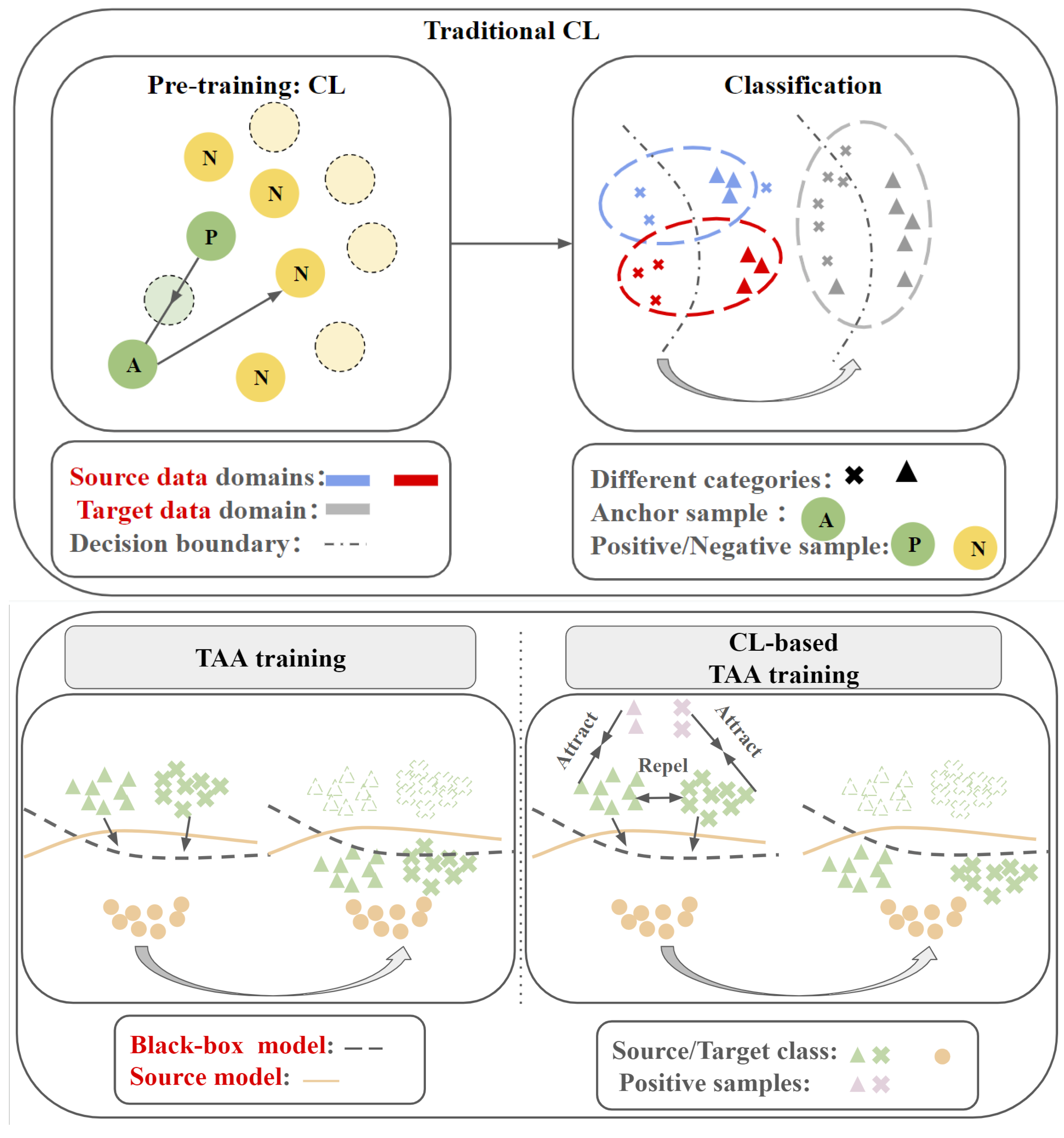
The illustration of the difference between traditional CL and our proposed CL-TAA is shown in
Figure 1. Contrastive learning is widely used in unsupervised learning to increase the model’s generalization to the unseen hard sample. In essence, contrastive learning is sophisticated in improving the model’s generalization by comparing the similarity between key and positive features and the differences between key and negative features. We conjecture that contrastive learning can also enhance the generalization of adversarial examples by comparing the similarity between key and positive features and the differences between key and negative features. Unlike previous works [
46], which utilize CL for visual representation to enhance the model’s generalization of the hard examples, our work specifically focuses on improving the generalization of adversarial examples. In other words, we aim to utilize CL to generate adversarial examples trained on a source model to attack a range of different black box models effectively. Another key distinction in our approach compared to previous studies is that we incorporate CL during the training process to optimize adversarial examples. Earlier works usually employed CL in the pre-training phase. Typically, CL is used in self-supervised settings, where models are trained on unlabeled data and then fine-tuned for downstream tasks. In our case, CL serves as a technique to improve the generalization of adversarial examples rather than for pre-training.
CL-based TAA Method. In the classical CL, three types of samples are typically involved: the anchor sample, positive sample, and negative samples, where these samples typically utilize the feature from the encoder. The anchor sample is sample of interest, and the positive samples are variations or augmentations derived from the anchor sample, while the negative samples are other randomly selected samples. We adopt the same practice in our work to generate the targeted adversarial examples, and what makes it different from the classical CL is the choice of these samples.
The common consensus is that DNNs are for feature extraction where logit values indicate the presence of the feature in the image, and the highest value in the logit is used for identifying the ground truth classes. The logit refers to the output feature of the model before the final softmax layer [
29]. In [
29], the authors demonstrate that the logit can be viewed as the features of the images. Since classical DNN models are typically designed without an encoder, we adopt logit for our CL. Specifically, we utilize the logit of the image as the anchor sample because it is the input of interest in this context. It has been demonstrated that the effect of adversarial examples is attributed to the governing of perturbation [
29]. To improve the perturbation dominance, we create the positive sample by blending a random clean image with the adversarial example. The InfoNCE [
16] loss has been used in multiple works and has become a de facto standard loss for CL; thus, we utilize InfoNCE in our work. Following the notation in [
45], we represent the logit of the anchor sample, positive sample, and negative sample as q, k+, and k−, respectively. To eliminate scale discrepancies, these logits are typically L2-normalized. Utilizing these normalized logits, InfoNCE loss applied in the contrastive learning-based TAA generation can be formulated as follows:
where
is the temperature controlling the sharpness or smoothness of the similarity distribution between feature vectors and thus affects how the model weighs positive and negative pairs when computing the loss. Unlike the classical CL method that generates the negative samples once and then saves them, we adopt the different negative samples for each iteration to increase the generalization of adversarial samples. In other words,
in Equation (
7) for each iteration is different for each iteration.
Practical Implementation. Contrastive learning requires a large number of SAR images for positive and negative samples, while SAR images are limited and expensive to obtain. To address this issue, we use the patches randomly cropped from the to-be-attacked clean image to generate the positive sample. For the negative samples, we randomly select the negative samples once and also use patches randomly cropped from these samples for each iteration. For these patches, we perform RandomResizedCrop in touchvision without considering the parameter of the random aspect ratio. We term our proposed method as CL-based targeted adversarial attack (CL-TAA); this method drastically reduces the usage of clean images. CL-TAA is summarized in Algorithm 1 and builds on the basic TAA method by incorporating a regularization term, which helps improve the generalization of adversarial examples. Following [
62], we set the maximum allowable perturbation magnitude to 16/255, with a step size of 2/255.
| Algorithm 1 CL-TAA |
Input: Source model ; input image x; images for negative samples ; target label ; allowed maximum perturbation magnitude ; total number of iterations T; step size ; hyperparameter of loss function ; cross-entropy loss function .
Output: Adversarial example with .
- 1:
; - 2:
for t = 0, 1, 2, ..., do - 3:
; ; - 4:
; - 5:
; - 6:
; - 7:
; - 8:
- 9:
- 10:
- 11:
end for - 12:
return .
|

 ,
, 


