Underwater Sonar Image Classification with Image Disentanglement Reconstruction and Zero-Shot Learning

Abstract

Sonar is a valuable tool for ocean exploration since it can obtain a wealth of data. With the development of intelligent technology, deep learning has brought new vitality to underwater sonar image classification. However, due to the difficulty and high cost of acquiring underwater sonar images, we have to consider the extreme case when there are no available sonar data of a specific category, and how to improve the prediction ability of intelligent classification models for unseen sonar data. In this work, we design an underwater sonar image classification method based on Image Disentanglement Reconstruction and Zero-Shot Learning (IDR-ZSL). Initially, an image disentanglement reconstruction (IDR) network is proposed for generating pseudo-sonar samples. The IDR consists of two encoders, a decoder, and three discriminators. The first encoder is responsible for extracting the structure vectors of the optical images and the texture vectors of the sonar images; the decoder is in charge of combining the above vectors to generate the pseudo-sonar images; and the second encoder is in charge of disentangling the pseudo-sonar images. Furthermore, three discriminators are incorporated to determine the realness and texture quality of the reconstructed image and feedback to the decoder. Subsequently, the underwater sonar image classification model performs zero-shot learning based on the generated pseudo-sonar images. Experimental results show that IDR-ZSL can generate high-quality pseudo-sonar images, and improve the prediction accuracy of the zero-shot classifier on unseen classes of sonar images.

1. Introduction

With the advancement of sonar technology, sonar facilitates the rapid acquisition of seafloor images and encompasses a plethora of valuable seafloor data. Underwater sonar image classification techniques have important research signification and broad application prospects, including marine rescue [1], marine resource conservation [2], archaeological excavations [3], and other related domains. In recent years, deep learning has gained widespread adoption across various domains due to its exceptional performance. Deep learning models efficiently and robustly acquire the feature information of samples, enabling accurate and effective classification of targets. Deep learning-based underwater sonar image classification has injected new vitality into this field, surpassing traditional algorithms in terms of efficiency and accuracy [4,5,6]. However, deep learning classification models require a substantial number of high-quality samples during the training process to effectively learn the target feature distribution and enhance its classification performance.

Because of the difficulty of the acquisition process, the number of available sonar images is seriously insufficient. In the case of limited samples, the issue of overfitting tends to arise during deep learning model training [7]. Specifically, the trained model may struggle to generalize well beyond the training data, leading to inaccurate predictions and compromised effectiveness [8]. In order to alleviate the above problems, many sonar image augmentation methods (such as HUO et al. [9], Seg2Sonar [10], MFA-CycleGAN [11], etc.) with excellent performance have been proposed. The diversity of sonar samples can be effectively increased by using the data augmentation approach to create new sonar samples through the application of different transforms. This approach can help to some extent with problems like overfitting and insufficient model classification accuracy.

However, when there are no available sonar data of a specific category, data augmentation methods are difficult to use for helping intelligent models train and classify such sonar targets in this extreme case. Therefore, the study of underwater sonar image classification without available training data is urgent and vital. This research can effectively improve the prediction ability of the model to the unknown sonar data, and has broad application prospects and value.

The existing research demonstrates that zero-shot learning (ZSL) can identify and classify unseen data from the training process [12]. Specifically, the knowledge acquired by ZSL through training data is effectively transferred to unseen categories, enabling accurate identification of unseen target images [13,14]. In comparison to supervised learning, which struggles with detecting rare or unknown samples, ZSL exhibits superior detection performance [15,16]. Although ZSL technology has developed rapidly in optical images, zero-shot learning for underwater sonar images still has a lot of room for improvement. Since sonar and optical images differ greatly from one another, applying the ZSL algorithm from the optical images field directly to the sonar images field is not effective.

To alleviate the above problems, we propose an underwater sonar image classification method based on image disentanglement reconstruction and zero-shot learning, namely IDR-ZSL. For the image disentanglement reconstruction stage, to reduce the domain gap between optical images and sonar images, we choose remote sensing images with a bird’s-eye view and known sonar images for generating pseudo-sonar images. Specifically, we disentangle the input sample based on the encoder to obtain its structure vector and texture vector. Subsequently, we combine the structural vector from optical images with the texture vector derived from sonar images to generate pseudo-sonar images based on the decoder. Regarding the zero-shot classification stage, we select certain categories from real sonar images as texture references in the pseudo-sonar image generated stage. These selected categories are excluded from the testing process. Subsequently, training is conducted using pseudo-sonar images. During testing, the classification model is evaluated and analyzed using real sonar images that do not appear in the training process to verify the performance of the zero-shot classification model. Overall, IDR-ZSL trains the zero-shot classification model by utilizing the pseudo-sonar images and enhancing the model’s predictive capability for unseen class samples. This research holds significant academic value and promising practical applications.

Our main contributions are as follows:

• We disentangle the images to integrate the structure vectors of optical images and the texture vectors of sonar images to generate a realistic pseudo-sonar image.
• We use the pseudo-sonar images to train the zero-shot classifier, aiming to enhance the detection performance of the classification model on unseen sonar images.
• We conducted comprehensive testing and analysis on the image generation and zero-shot classification, and the experimental results demonstrate the method we propose has good performance in underwater sonar image classification.

The remaining sections of the paper are organized as follows: Section 2 presents a review of the existing literature on underwater sonar image classification methods, while Section 3 elaborates on the detailed design of IDR-ZSL, and Section 4 conducts comprehensive experiments and analysis, followed by a discussion and conclusion in Section 5 and Section 6.

2. Related Work

2.1. Sonar Image Object Classification

Underwater sonar image object classification based on deep learning has been extensively studied because of its exceptional performance. Compared with the traditional algorithm, the intelligent classification model can efficiently and accurately predict the underwater target and offers improvements in many indicators. Therefore, deep learning has brought new vitality to underwater object classification. Preciado-Grijalva et al. [17] proposed a sonar image classification method based on self-supervised learning, which does not require a large number of labeled datasets for training and reduces the dependence on sonar samples, and three self-supervised methods (RotNet, Denoising Autoencoders, and Jigsaw) are fully studied and analyzed. Experimental results indicate that the classification performance is comparable to that of supervised learning, thereby offering a viable feature learning approach for underwater intelligent perception. Gerg et al. [18] proposed a deep learning architecture based on prior knowledge for synthetic aperture sonar image classification. Structured Prior Driven Regularized Deep Learning (SPDRDL) integrates prior knowledge into convolutional neural networks to further improve sonar image classification performance without additional training data. Specifically, Gerg et al. introduces two structural prior knowledge frameworks: Structural Similarity Prior (SSP) and Structural Scene Context Prior (SSCP). Compared to other intelligent underwater classification algorithms, SPDRDL effectively reduces the false positive rate and improves overall accuracy. This research demonstrates that integrating prior knowledge can substantially enhance classification performance, offering a novel approach for underwater target classification. HUO et al. [9] used transfer learning based on pre-trained deep convolutional networks to classify real sonar data. This work established the real sonar image dataset SeabedObjects-KLSG. Furthermore, to address the imbalance in the dataset, HUO et al. introduce a semi-synthetic sonar image generation method based on optical image segmentation. The experimental results show that transfer learning and image synthesis can effectively enhance the performance of target classification. Wang et al. [19] proposed an underwater sonar image classification model based on adaptive weight convolutional neural networks, using the weights of deep belief networks to adaptively replace the weights of convolutional neural network filters. Experimental results show that this method has good classification performance.

2.2. Sonar Image Augmentation

The existing research shows that convolutional neural networks (CNNs) have excellent performance in the field of underwater object classification. Unfortunately, the CNN model requires a large number of training samples to successfully learn the depth features of various types of samples and perform reliable detection and recognition. When the training sample is insufficient, the network is at risk of overfitting, preventing effective generalization and making it difficult to accurately predict the test sample. However, the underwater sonar image does not have enough available data due to the difficulty of acquiring such data, and the high cost of doing so, making it challenging to provide efficient data support for the subsequent underwater target detection, recognition, and segmentation tasks. Many high-performing sonar image augmentation methods have been proposed, inspired by optical sample augmentation techniques. The sample augmentation approach increases the number of sonar training samples, reduces the cost and difficulty of sonar sample acquisition, provides data support for intelligent model training, and in part mitigates the issue of overfitting by generating realistic pseudo-sonar images. Huang et al. [10] proposed a Seg2Sonar network based on spatially adaptive denormalization, including a skip-layer channel-wise excitation module, focal frequency loss module, elasticity loss strategy, and weight adjustment strategy. Specifically, the skip-layer channel-wise excitation module is employed to augment the feature extraction capability. The focal frequency loss module and elastic loss strategy are introduced to enhance the quality of the synthesis image. Furthermore, a weight adjustment strategy is proposed to address the imbalance in the feature distribution. This method can effectively transform the segmentation images into sonar images, and provide effective sample enhancement for subsequent detection, recognition, and segmentation based on deep learning. Yang et al. [20] proposed a side-scan sonar image sample enhancement method adapted to multi-task scenarios. Specifically, the method migrates a diffusion model pre-trained in an optical image to a side-scan sonar image. The guide information of the diffusion model includes image content and target shape. Experimental results show that the image synthesized by this method can effectively improve the accuracy of underwater target detection and segmentation tasks. Huang et al. [21] proposed a comprehensive sample enhancement method for side-scan sonar images, which integrates the imaging mechanisms of acoustic emission and reception, waterbody, target reflection, and seafloor background into the sample enhancement process. The experimental results show that the detection accuracy of the object detection module YOLOv5s can be effectively improved based on the side-scan sonar images generated in the work. Zhou et al. [11] proposed a sample synthesis method for converting remote sensing images into sonar images based on the multigranular feature alignment cycle-consistent generative adversarial network. Specifically, the method preserves the unique features of the image through the spatial attention-based feature aggregation module and introduces a pair of cross-domain discriminators to guide the model to generate a sonar-style image. In addition, the cycle consistency loss based on the discrete cosine transform is added to make better use of the characteristics in the frequency domain. The experimental results demonstrate the effectiveness of the proposed method, which provides an effective data enhancement strategy for underwater target detection and helps to improve the perception ability of AUVs in complex underwater environments.

2.3. Zero-Shot Learning

The sample augmentation technique can alleviate the overfitting problem to some extent. However, when there are no underwater sonar images available for model training, it is difficult to assess the effectiveness of the sample augmentation method. Due to the particularity of underwater sonar images, underwater object classification has to consider the solutions for the above extreme cases. Existing studies demonstrate that zero-shot learning can effectively transfer knowledge learned from known data to unknown data, and improve the prediction power of rare and unknown samples. Zero-shot learning has low dependence on the datasets and has shown great application potential in many fields. Chen et al. [22] propose a novel zero-shot learning method that aims to improve the performance of ZSL by explicitly discovering semantically relevant visual representations and discarding semantically irrelevant visual information. This method achieves accurate visual–semantic interaction and significant performance improvement in zero-shot learning tasks. In order to alleviate the poor effect of existing zero-shot learning on dissimilar unseen classes, Li et al. [23] introduce diversified semantic information from external classes and introduce external semantics into visual space through pre-training networks. This method can be robust when it comes to similar and dissimilar invisible classes, and improve the generalization ability of different unknown classes effectively. Hou et al. [24] propose a visual-augmented dynamic semantic prototype approach to facilitate the generator to learn the mappings of semantics and visuals effectively. The method is composed of a visual-aware domain knowledge learning module and vision-oriented semantic updation module. Experimental results show that the average performance of the method is improved effectively in multiple datasets.

ZSL technology is developing quickly in optical imaging, and its efficacy has been thoroughly examined. However, sonar and optical images have great differences, and it is challenging to apply efficient ZSL technology in the optical field to sonar images directly; instead, it must be further adjusted and improved. Li et al. [25] designed a zero-shot classification method of side-scan sonar images based on style transfer. Specifically, the method converts the optical image to a pseudo-sonar image in the style of a sonar image. The zero-shot classifier is then trained based on the generated pseudo-sonar images. Experimental results on real sonar data demonstrate that this method has good classification performance.

The above method uses the style transfer technique to convert optical images to pseudo-sonar images for zero-shot training, but does not consider the inherent properties of optical images and sonar images. In this work, we fully consider the inherent properties of images, such as image structure and texture. Specifically, the structure of the optical image is combined with the texture of the known sonar image to generate the pseudo-sonar image, which helps the intelligent classification model to conduct zero-shot training.

3. Proposed Method

3.1. Framework Overview

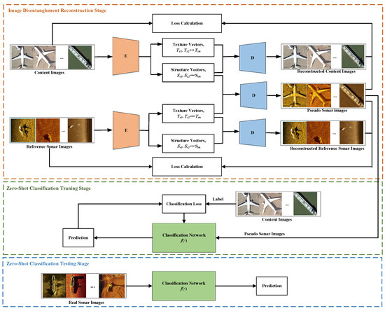
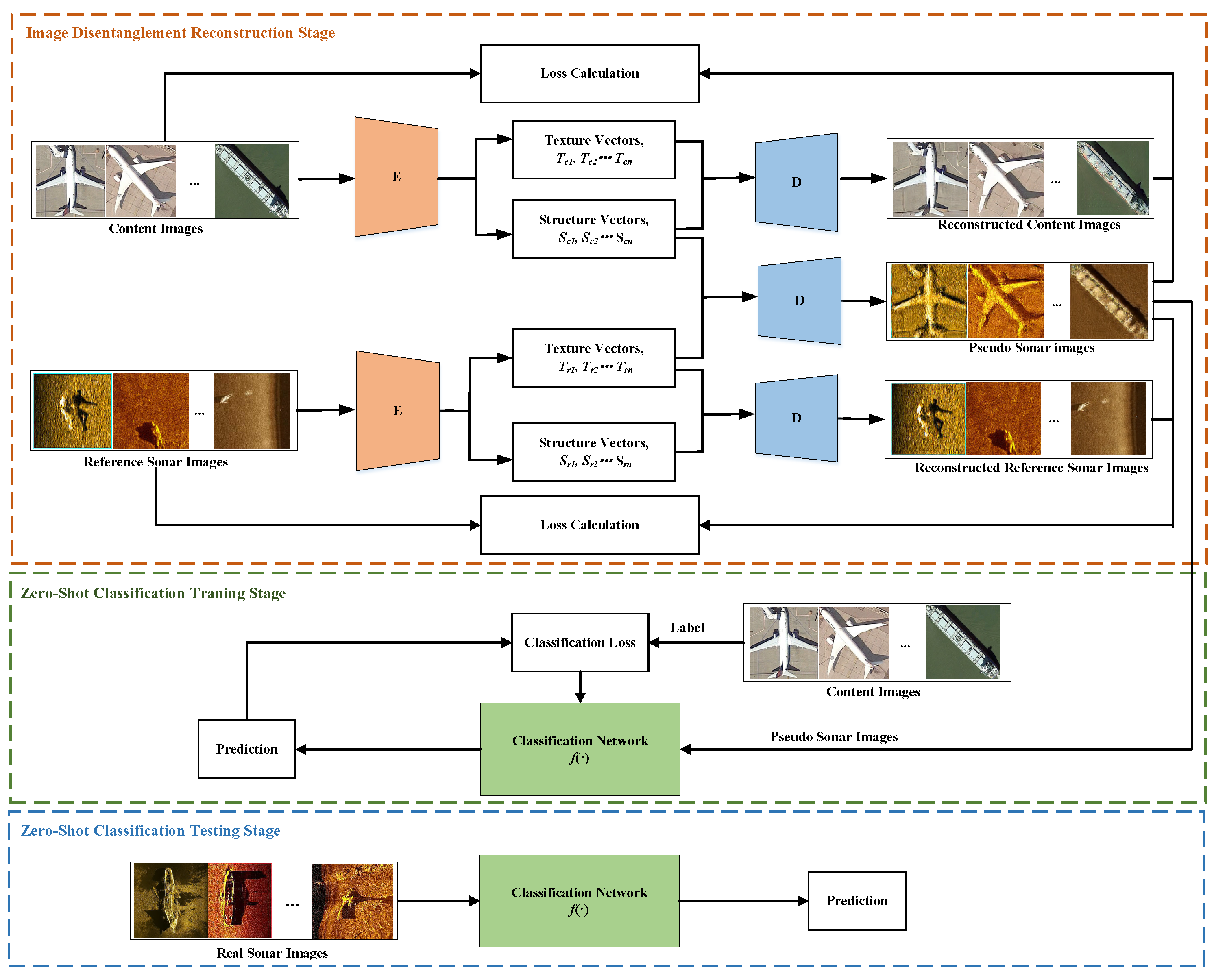
In this work, we propose an underwater sonar image classification method based on image disentanglement reconstruction and zero-shot learning, namely IDR-ZSL. The notation used in this work is shown in Table 1, and the framework of IDR-ZSL is shown in Figure 1. Regarding image disentanglement reconstruction, we use an encoder to disentangle the content images and reference sonar images to obtain texture and structure vectors. Subsequently, pseudo-sonar images are generated from the structure vectors of the content images and the texture vectors of the reference sonar image. In zero-shot learning, it is worth noting that certain categories (e.g., human and background) are chosen as the reference sonar images in the reconstruction stage, and the real sonar images of these categories will no longer be present in the zero-shot classification training and testing stage. Specifically, pseudo-sonar images are input to the classification network for training, enabling the classifier to acquire knowledge of the sample features to improve the prediction performance. In the test stage, real sonar images of previously unseen categories are input to verify the zero-shot learning effect of the classification network.

Table 1. The notation used in this work.

Notation	Description
E	The encoder of content image and reference sonar image
$E_2$	The encoder of pseudo-sonar image
D	The decoder
$D_{co1}$	The co-occurrence discriminator of sonar image
$D_{co2}$	The co-occurrence discriminator of optical content image
$D_{real}$	The discriminator that identifies the authenticity of the input image
S	The image structure vector extracted by the encoder
T	The image texture vector extracted by the encoder
$X_c$	The optical content image
${\tilde{X}}_c$	The reconstructed optical content image
$X_r$	The reference sonar image
${\tilde{X}}_r$	The reconstructed reference sonar image
${\tilde{X}}_{cr}$	The generated pseudo-sonar images
$X_s$	The real sonar images

Figure 1. The framework of IDR-ZSL.

3.2. Image Disentanglement Reconstruction

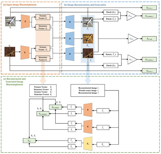
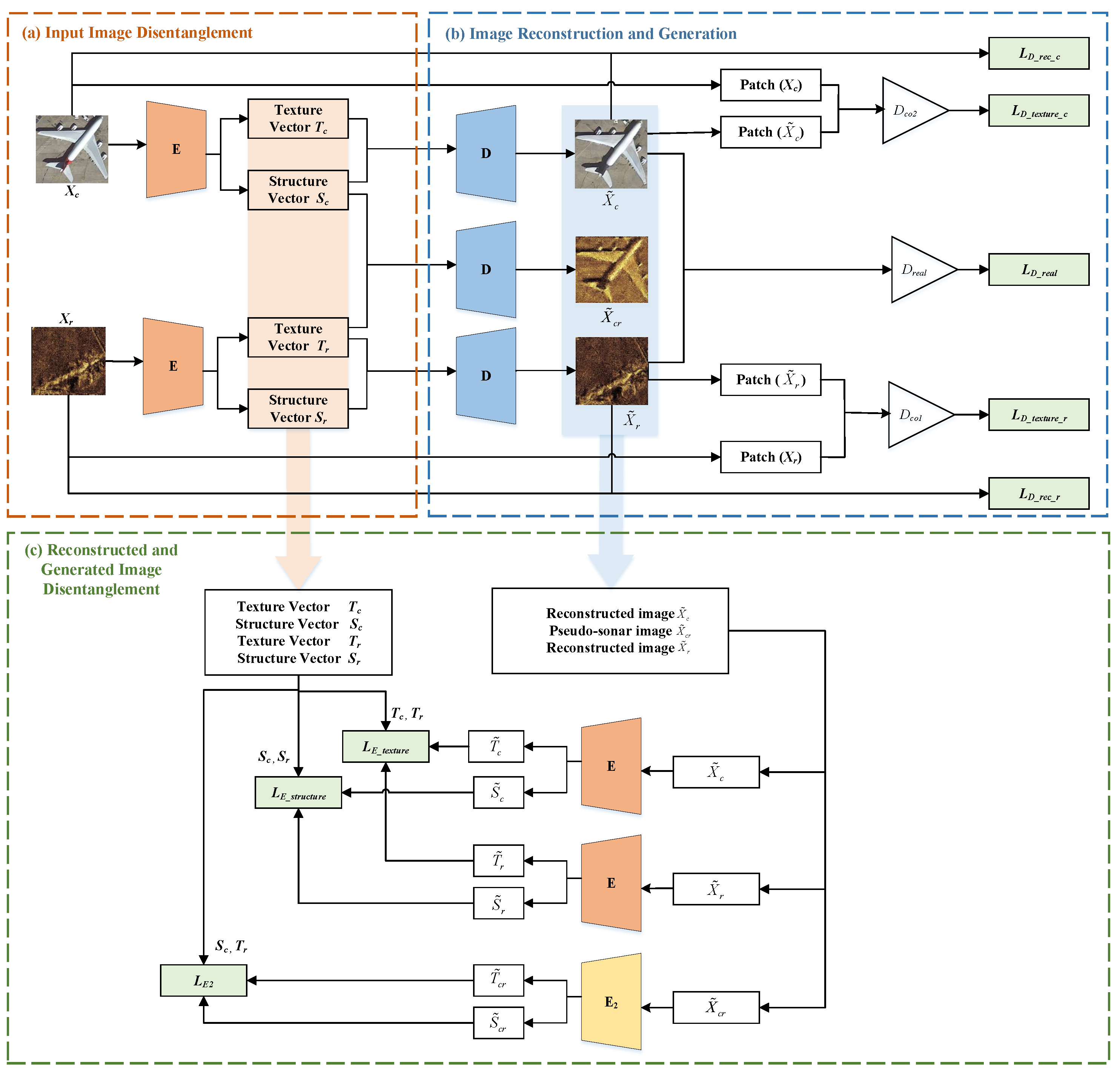
We employ IDEAS [26] as our backbone network to enhance the performance of pseudo-sonar image generation. It is worth noting that the core network of IDEAS is styleGAN2 [27], which can synthesize high-resolution and high-fidelity images, but many samples are needed for learning in the training process. However, the limited sonar image makes it difficult to meet the training requirements of StyleGAN2, which can easily cause the discriminator to overfit, so the discriminator cannot provide effective information for the generator to synthesize fake images. To avoid the above problems, we modify IDEAS to obtain the Image Disentanglement Reconstruction (IDR) network, which does not synthesize fake images from random latent spaces but uses the reconstruction of existing sonar images and remote sensing images to obtain fusion reconstructed images. Specifically, the IDR network comprises two encoders, a decoder, and three discriminators, as illustrated in Figure 2. The IDR training process is divided into three stages: input image disentanglement, image reconstruction and generation, and reconstructed and generated image disentanglement. (a) In the input image disentanglement stage, the encoder disentangles the input image to obtain texture and structure vector. (b) In the image reconstruction and generation stage, decoder D will reconstruct and generate the images based on the input structure and texture vectors to obtain ${\tilde{X}}_c$, ${\tilde{X}}_s$, and ${\tilde{X}}_{cr}$. (c) In the reconstructed and generated image disentanglement stage, the encoders E and $E_2$ disentangle the reconstructed image and generated pseudo-sonar image, respectively, extract the structure and texture vectors, and compare them with the vectors obtained in stage (a).

Figure 2. Flow chart of image disentanglement reconstruction.

3.2.1. Input Image Disentanglement

The encoder E disentangles the input samples $X_c$ and $X_r$ first:

$$(S_c,T_c)=E\left(X_c\right)$$

(1)

$$(S_r,T_r)=E\left(X_r\right)$$

(2)

where $S_c$ and $T_c$ are the decoupling vectors of $X_c$, and $S_r$ and $T_r$ are the decoupling vectors of $X_r$.

3.2.2. Image Reconstruction and Generation

The decoder D reconstructs images and generates pseudo-sonar images based on the above image structure and texture vectors:

$${\tilde{X}}_c=D(S_c,T_c)$$

(3)

$${\tilde{X}}_r=D(S_r,T_r)$$

(4)

$${\tilde{X}}_{cr}=D(S_c,T_r)$$

(5)

where ${\tilde{X}}_c$ and ${\tilde{X}}_r$ are the reconstructed samples, and ${\tilde{X}}_{cr}$ is the generated pseudo sonar image. The reconstruction loss between input samples and reconstructed samples is as follows:

$$L_{D\_rec}=\parallel {\tilde{X}}_c-X_c{\parallel }_1+{\parallel {\tilde{X}}_r-X_r\parallel }_1$$

(6)

where ${\parallel ·\parallel }_1$ means the $L1$ loss between images.

Additionally, IDR uses the discriminator $D_{co1}$ and $D_{co2}$ to provide feedback on the texture quality of reconstructed samples. Specifically, $D_{co1}$ and $D_{co2}$ are the co-occurrence discriminators [28] used to compare texture similarities. $D_{co1}$ randomly selects the patches of $X_r$ and ${\tilde{X}}_r$ to identify the similarity of the textures. $D_{co2}$ randomly selects the patches of $X_c$ and ${\tilde{X}}_c$ to identify the similarity of the textures. The texture similarity between the input image and the reconstructed image is calculated based on the discriminator $D_{co1}$ and $D_{co2}$, as follows:

$$L_{D\_texture\_r}=D_{co1}(patch\left({\tilde{X}}_r\right),patch\left(X_r\right))$$

(7)

$$L_{D\_texture\_c}=D_{co2}(patch\left({\tilde{X}}_c\right),patch\left(X_c\right))$$

(8)

$$L_{D\_texture}=L_{D\_texture\_r}+L_{D\_texture\_c}$$

(9)

where $patch(·)$ is the random cropping function.

Furthermore, IDR uses $D_{real}$ to identify the reality of the input sample, and the reality loss is as follows:

$$L_{D\_real}=D_{real}\left({\tilde{X}}_c\right)+D_{real}\left({\tilde{X}}_r\right)$$

(10)

Consequently, the loss of the decoder is as follows:

$$L_D=L_{D\_rec}+L_{D\_texture}+L_{D\_real}$$

(11)

3.2.3. Reconstructed and Generated Image Disentanglement

The reconstructed sample should exhibit a high degree of similarity to the original input sample, and the structure and texture vectors of ${\tilde{X}}_c$ and ${\tilde{X}}_s$ should also be close to those vectors of the input sample. To facilitate comparison, we disentangle the reconstructed sample ${\tilde{X}}_c$ and ${\tilde{X}}_r$ based on the encoder E:

$$({\tilde{S}}_c,{\tilde{T}}_c)=E\left({\tilde{X}}_c\right)$$

(12)

$$({\tilde{S}}_r,{\tilde{T}}_r)=E\left({\tilde{X}}_r\right)$$

(13)

The structure vector loss between the original sample and the reconstructed sample is as follows:

$$L_{E{\_}_{structure}}=\parallel {\tilde{S}}_c-S_c{\parallel }_1+{\parallel {\tilde{S}}_r-S_r\parallel }_1$$

(14)

The texture vector loss between the original sample and the reconstructed sample is as follows:

$$L_{E{\_}_{texture}}=\parallel {\tilde{T}}_c-T_c{\parallel }_1+{\parallel {\tilde{T}}_r-T_r\parallel }_1$$

(15)

Consequently, the loss of the encoder is as follows:

$$L_E=L_{E{\_}_{structure}}+L_{E{\_}_{texture}}$$

(16)

Regarding pseudo-sonar sample ${\tilde{X}}_{cr}$, its structure and texture vector should ideally be infinitely close to the structure of the optical content image and the texture of the reference sonar image, respectively. To facilitate comparison, we disentangle the generated pseudo-sonar sample ${\tilde{X}}_{cr}$ based on the encoder $E_2$:

$$({\tilde{S}}_{cr},{\tilde{T}}_{cr})=E_2\left({\tilde{X}}_{cr}\right)$$

(17)

The structure of the $S_{cr}$ sample is expected to be consistent with that of the optical content image, so the structure vector loss of $E_2$ is the following:

$$L_{E_2{\_}_{structure}}={\parallel {\tilde{S}}_{cr}-S_c\parallel }_1$$

(18)

The texture of the $S_{cr}$ sample is expected to be consistent with that of the reference sonar image, so the texture vector loss of $E_2$ is the following:

$$L_{E_2{\_}_{texture}}={\parallel {\tilde{T}}_{cr}-T_r\parallel }_1$$

(19)

Consequently, the loss of the encoder $E_2$ is as follows:

$$L_{E_2}=L_{E_2{\_}_{structure}}+L_{E_2{\_}_{texture}}$$

(20)

Based on the analysis of the above three stages, the IDR loss is as follows:

$$L_{IDR}=L_D+L_E+\alpha L_{E_2}$$

(21)

where $\alpha$ means the weight parameter.

3.3. Zero-Shot Classification

3.3.1. Data Preparation

During the process of zero-shot learning, the knowledge acquired from the pseudo-sonar sample is transferred to unseen classes of real sonar images, thereby enhancing classification performance for unseen samples. The dataset used for this process is shown in Table 2.

Table 2. Datasets utilized for zero-shot classification.

Stage	Dataset	Describe	Category	Number	Total
Pseudo-sonar image generation stage	$K_c$ [29]	The optical content images provide structured vectors for the subsequent ${\tilde{X}}_{cr}$ generation.	Aircraft	1000	3800
			Ship	1000
			Others	1800
	$K_r$ (SCTD) [30]	The reference sonar images provide texture vectors for the subsequent ${\tilde{X}}_{cr}$ generation.	Human	44	110
			Background	66
Real sonar image testing stage	KLSG [9]	Real sonar images for testing the zero-shot classifier.	Aircraft	62	447
			Shipwreck	385
	SCTD [30]	Real sonar images for testing the zero-shot classifier.	Aircraft	90	453
			Shipwreck	363

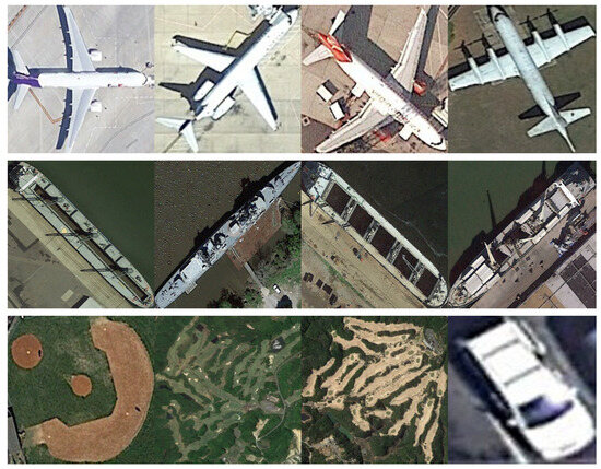
There are huge differences between sonar images and optical images, and reducing the gap between them is one of the keys to zero-shot learning. Therefore, remote sensing images with a bird’s-eye view are used to alleviate the above problems. Specifically, remote sensing images are obtained from the DIOR [29] dataset, whose samples usually contain multiple targets. In order to better complete the image fusion reconstruction task, we need to preprocess the dataset and extract the targets contained in the samples. The annotation file provided by the dataset can be used to obtain coordinate information for various targets in the sample, allowing the target to be extracted and saved as an image. The DIOR dataset contains multiple categories of images. In order to better fit the zero-sample classification task of subsequent sonar images, we selected 1000 images of the aircraft, 1000 images of the ship, and 1800 images of other categories (including the baseball field, golf field, and vehicle), and a total of 3800 remote sensing images formed the $K_c$ dataset to provide structural vectors for the subsequent generation of pseudo-sonar images. Examples of the optical content images are shown in Figure 3.

Figure 3. Examples of the optical content images. The first row is four examples of the aircraft category, the second row is four examples of the ship category, and the third row is four examples of the other categories, including baseball field, golf course, and vehicle.

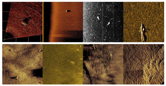
In addition, we use the human image and the intercepted background image, (which do not contain sonar targets), in the SCTD [30] dataset as known sonar data to form the reference sonar image dataset $K_r$. This dataset provides texture vectors for the subsequent generation of pseudo-sonar images. However, there is a large gap between the number of $K_r$ and $K_c$, which can easily affect the training effect of the IDR model. Therefore, the further data augmentation of the $K_r$ dataset is necessary. In the process of augmentation, we need to consider the problem of data leakage to avoid affecting the effect of the pseudo-sonar image. We choose four data augmentation methods—rotation 90 degrees, rotation 180 degrees, horizontal flip, and blur—to expand the category of human. In addition, the background image is augmented by rotating 90 degrees and 180 degrees. The expanded $K_r$ dataset included 220 human images and 198 background images. Examples of the reference sonar images are shown in Figure 4.

Figure 4. Examples of the reference sonar images. The first row is four examples of the human category, and the second row is four examples of the background category.

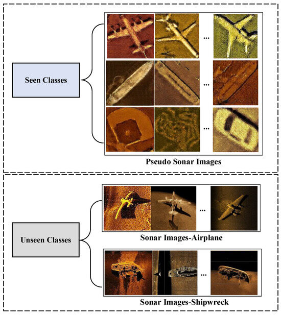
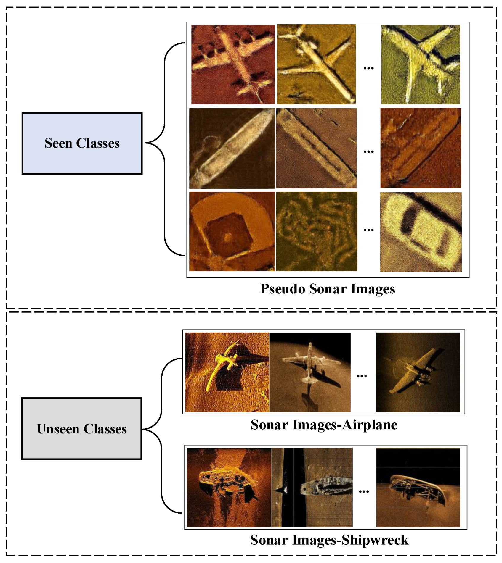
The seen and unseen classes of the ZSL training and testing process are shown in Figure 5. The seen classes are pseudo-sonar images, which are generated by the IDR model. During the testing phase, the real sonar data of airplane and shipwreck categories in KLSG [9] and SCTD datasets are selected to verify the zero-shot classification performance of the classifier on the unseen categories.

Figure 5. The seen and unseen classes of the ZSL training and testing process.

3.3.2. Algorithm of Zero-Shot Learning

The IDR-ZSL algorithm is primarily composed of the training stage and testing stage, as shown in Algorithm 1. Specifically, the content images and corresponding labels are loaded from the dataset $K_c$, and the reference sonar image $X_r$ is loaded from the $K_r$ datasets. Moreover, the IDR module is employed to disentangle the input images, and the pseudo-sonar image ${\tilde{X}}_{cr}$ is generated based on the structure vector of the content image and the texture vector of the reference sonar image. In addition, the labels of ${\tilde{X}}_{cr}$ are consistent with that of the content images. Afterward, the pseudo-sonar image dataset $K_{cr}$ is obtained. The sonar image classifier loads the $K_{cr}$ dataset for training, calculates the loss function, and updates the model weight. In the test phase, IDR-ZSL loads the real sonar datasets KLSG and SCTD to evaluate the detection performance and effectiveness of the model on the unseen sonar images.

Algorithm 1 The algorithm of zero-shot learning.

Input: epoch, trained IDR model, $K_c$, $K_r$, KLSG and SCTD Output: Accuracy   1: Training Stage   2: Load samples and labels $\{X_c,Y_c\}$ from $K_c$   3: Load samples $\left\{X_r\right\}$ from $K_r$   4: Load E and D from the trained IDR model   5: N ⇐ the number of $\left\{X_c\right\}$   6: for $i=0$ to N do   7:    $(S_c,T_c)\Leftarrow E\left(X_c\right)$   8:    $(S_r,T_r)\Leftarrow E\left(X_r\right)$   9:     ${\tilde{X}}_{cr}\Leftarrow D(S_c,T_r)$ 10:     ${\tilde{Y}}_{cr}\Leftarrow Y_c$ 11: end for 12: Pseudo-sonar image dataset $K_{cr}$⇐$\{{\tilde{X}}_{cr},{\tilde{Y}}_{cr}\}$ 13: Load samples and labels $\{{\tilde{X}}_{cr},{\tilde{Y}}_{cr}\}$ from $K_{cr}$ 14: Threshold $\Leftarrow 0$ 15: for $i=0$ to epoch do 16:    Predictions ⇐ $f\left({\tilde{X}}_{cr}\right)$ 17:    Accuracy ⇐ compare Predictions and ${\tilde{Y}}_{cr}$ 18:    if Accuracy > Threshold then 19:       Threshold ⇐ Accuracy 20:       Update the network weights of $f(·)$ 21:     end if 22: end for 23: Testing stage 24: Load samples and labels $\{X_s,Y_s\}$ from KLSG or SCTD 25: N ⇐ the number of $\left\{X_s\right\}$ 26: for $i=0$ to N do 27:    Predictions ⇐$f\left(X_s\right)$ 28:    Accuracy ⇐ compare Predictions and $Y_s$ 29: end for 30: return Accuracy

4. Experiment

4.1. Experiment Setup

We evaluate the performance of IDR-ZSL on a server with the Intel (R) Xeon (R) Gold 6226R CPU and NVIDIA GeForce RTX 3090 GPU. The datasets employed in the experimental training and test stage included optical content samples of $K_c$, reference sonar samples of $K_r$, and real sonar samples of KLSG and SCTD. The specific categories and sample numbers of these datasets are presented in Table 2.

As for the specific experiment process, we initially reconstructed optical remote sensing images and reference sonar images to evaluate the IDR’s disentanglement reconstruction capability. Additionally, we generated pseudo-sonar images to visually evaluate them intuitively. Furthermore, the reconstructed images and generated pseudo-sonar images were assessed utilizing Inception Score (IS) [31], Fréchet Inception Distance (FID) [32], and Kernel Inception Distance (KID) [33] metrics to compare and analyze the image quality objectively. Regarding the zero-shot classification, the ResNet-34 [34], ResNet-152 [34], VGG-19 [35], DenseNet-121 [36], AlexNet [37], GoogleNet [38], SqueezeNet [39], and MobileNetV2 [40] models were employed as the classifier. The performance of the zero-shot classifiers was evaluated using global accuracy and average accuracy metrics, enabling a comparative analysis of the classification capabilities among different models.

4.2. Image Disentanglement Reconstruction

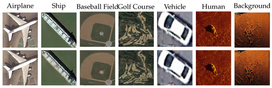
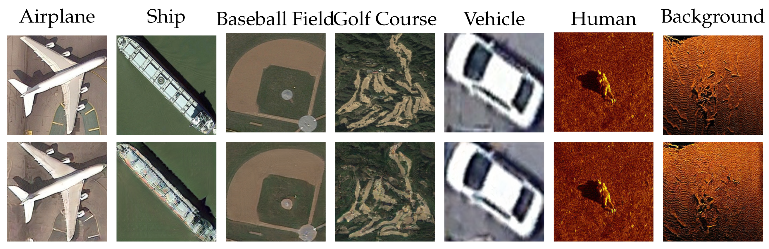
The disentanglement reconstruction effects of IDR can be effectively verified by comparing the reconstructed image with the original image. Only when IDR can accurately disentangle the image can the image be effectively reconstructed based on the disentanglement structure and texture vector. As shown in Figure 6, the reconstructed images of IDR are almost consistent with the original images for the classes of the baseball field, vehicle, and human. However, for images of the airplane, ship, golf field, and background categories, there are slight differences in texture and structure between the reconstructed images and the original images, which may be because the images are more complex than those of other categories.

Figure 6. Disentanglement reconstruction effect of optical content image $X_c$ and reference sonar image $X_r$. The optical content images for columns 1 to 5 are from the DIOR dataset [29], and the reference sonar images for columns 6 to 7 are from the SCTD dataset [30].

In the process of the quantitative evaluation of the quality of disentanglement reconstruction, we selected 1000 samples for each category of $X_c$ for testing. Regarding $X_r$, since there were too few sonar reference images, data augmentation was required before evaluation. Human images were augmented by rotation of 90 degrees, rotation of 180 degrees, horizontal flipping, and blur. The background images were augmented by rotation of 90 and 180 degrees. The number of human and background samples after data augmentation were 220 and 198, respectively. The test results are shown in Table 3. Obviously, the disentanglement reconstruction quality of $X_c$ performs better in the IS metric, indicating that the reconstructed image ${\tilde{X}}_c$ has a high diversity. However, the reconstructed images of $X_r$ perform better in the FID and KID metrics. The FID and KID metrics measure the difference in the distribution of images in the feature space, where the KID metric is more sensitive to second-order differences in distribution than the FID metric. Lower FID and KID values indicate that the statistical characteristics of ${\tilde{X}}_r$ in the feature space are closer to those of $X_r$ and have a better authenticity.

Table 3. Quantitative evaluation of reconstruction quality of optical content image and reference sonar image.

Image	Image Category	IS ↑	FID ↓	KID ↓
$X_c and {\tilde{X}}_c$	Ship	3.0442	109.8039	0.0983
	Airplane	5.2340	118.0901	0.0615
	Others	4.2403	114.5206	0.0504
	AVG	4.1728	114.1382	0.0701
$X_r and {\tilde{X}}_r$	Human	3.9668	109.8945	0.0133
	Background	3.4383	89.5107	0.0050
	AVG	3.7026	99.7026	0.0092

4.3. Pseudo-Sonar Image Generation

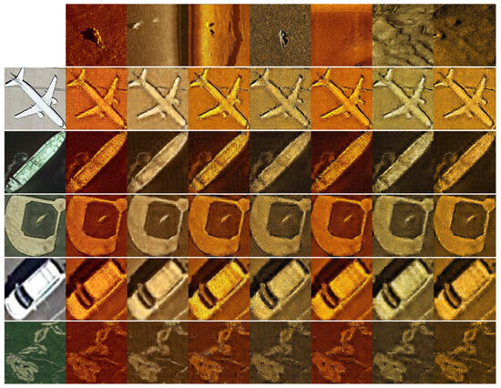
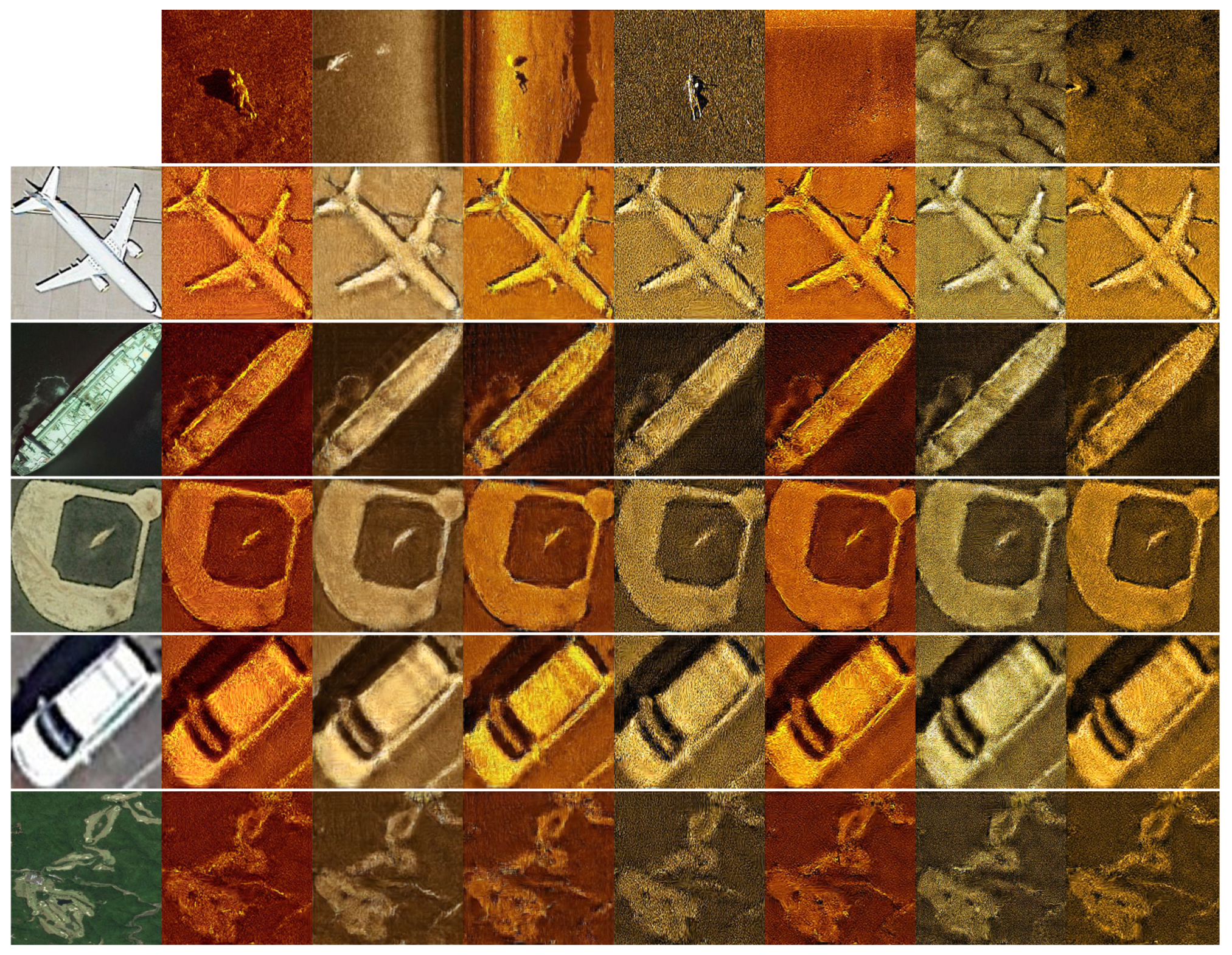
The quality evaluation of the generated pseudo-sonar images will be conducted in this section. Specifically, we generate pseudo-sonar images to conduct an intuitive evaluation of image quality. In the comparison of generated images, we select seven real images from the reference sonar dataset $K_r$ to extract the texture vectors. Moreover, we randomly select five images from the optical content image dataset $K_c$ to extract the structure vectors. Furthermore, the pseudo-sonar images ${\tilde{X}}_{cr}$ are generated based on the pairwise combination of the above texture and structure vectors, as shown in Figure 7. The pseudo-sonar images maintain the structure of the optical image while also having the textural details of the referenced sonar image. For example, the structure of the pseudo-sonar images in rows 2, 4, and 5 of Figure 7 is almost consistent with that of the first column of aircraft, baseball field, and vehicle images. Meanwhile, these pseudo-sonar images can effectively integrate the texture information of the first row of human and background reference sonar images. However, the structure of the pseudo-sonar images in rows 3 and 6 of Figure 7 are roughly the same as the ship and golf course in the first column, but there are subtle structural differences. This may be due to the complex structure of the ship and golf course images. In conclusion, ${\tilde{X}}_{cr}$ performs well visually, and can effectively establish the foundation for the training of zero-shot classifying.

Figure 7. Pseudo-sonar images generated by IDR. The first row is seven real sonar images selected from the reference sonar dataset, the first column is five images randomly selected from the optical content image dataset, and the remaining images are the generated pseudo-sonar images.

We conducted an ablation study to understand each network’s function and value in the model. Table 4 shows specific experimental settings. Networks E, $E_2$, and D are the basic networks for completing the generation of pseudo-sonar images, while $D_{co1}$, $D_{co2}$, and $D_{real}$ networks are used for adversarial training to increase the quality of images. Consequently, we set up three models—$E+E_2+D+D_{co1}$, $E+E_2+D+D_{co2}$, and $E+E_2+D+D_{real}$—to compare the IDR model with for evaluating the function of the three discriminators.

Table 4. Ablation study experiment setup.

Model	E	${\mathit{E}}_2$	D	${\mathit{D}}_{\mathit{co}1}$	${\mathit{D}}_{\mathit{co}2}$	${\mathit{D}}_{\mathit{real}}$
RM1 ($E+E_2+D+D_{co1}$)	√	√	√	√
RM2 ($E+E_2+D+D_{co2}$)	√	√	√		√
RM3 ($E+E_2+D+D_{real}$)	√	√	√			√
IDR	√	√	√	√	√	√

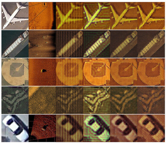
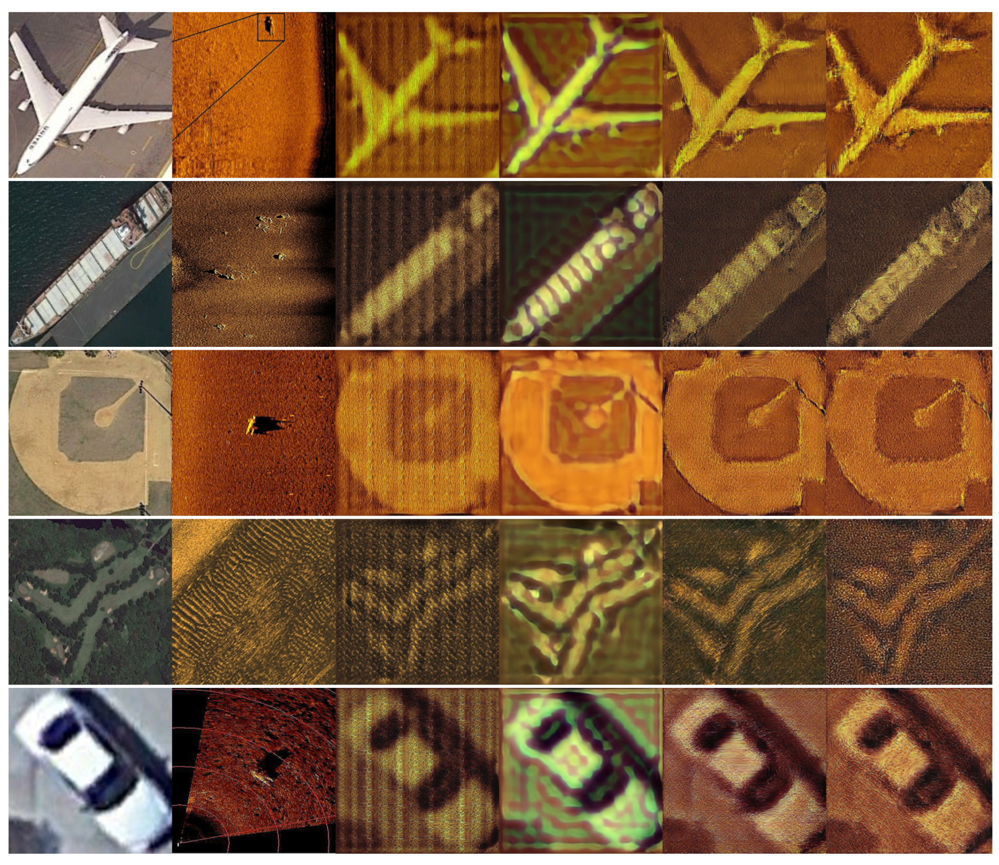
In addition, the pseudo-sonar images generated by the four groups of models in the ablation study are shown in Figure 8. RM1 only adds the $D_{co1}$ network to the basic network $E+E_2+D$; we can see that the texture of $X_{cr}$ is similar to that of $X_r$, but the structure is fuzzy. This is because $D_{co1}$ compares the texture similarity of $X_r$ and ${\tilde{X}}_r$ in the training process, as shown in Formula (7). Therefore, $D_{co1}$ can help the model effectively learn the texture features of the reference sonar image, while the learning of the optical content image is insufficient. When RM2 adds the $D_{co2}$ network to the basic network, the structure of the $X_c$ can be better represented, but it could not effectively learn the texture information of the sonar image. This is because $D_{co2}$ compares the texture similarity of $X_c$ and ${\tilde{X}}_c$ in the training process, as shown in Formula (8). Therefore, $D_{co2}$ can assist the model learn the feature information of the $X_c$ image, but it cannot efficiently learn the texture of the $X_r$ image. RM3 adds the $D_{real}$ network to the basic network, and the reality of the reconstructed ${\tilde{X}}_c$ and ${\tilde{X}}_r$ may be efficiently determined. Encoder E can extract the structure of $X_c$ and the texture of $X_r$ more accurately, resulting in a higher-quality reconstructed ${\tilde{X}}_{cr}$. Compared to the first three groups of reference models, the IDR model incorporates the $D_{co1}$, $D_{co2}$, and $D_{real}$ discriminator networks, and the structure and texture features of reconstructed ${\tilde{X}}_{cr}$ are more similar to the original sonar image.

Figure 8. Comparison of pseudo-sonar images generated by different models. Column 1 is the optical content images, column 2 is the sonar images, and columns 3 to 6 are the pseudo-sonar images generated by the RM1 ($E+E_2+D+D_{co1}$), RM2 ($E+E_2+D+D_{co2}$), RM3 ($E+E_2+D+D_{real}$), and IDR models, respectively.

4.4. Quantitative Evaluation of Pseudo-Sonar Image Quality

The IS, FID, and KID metrics are employed in this section to quantitatively compare and analyze the performance of IDR methods in terms of image reconstruction quality, as presented in Table 5. Specifically, we compare the pseudo-sonar images ${\tilde{X}}_{cr}$ generated by the four models (e.g., RM1, RM2, RM3, IDR) with the real sonar images. ${\tilde{X}}_{cr}$ was generated based on sonar reference images of $K_r$ datasets and optical images of the $K_c$ dataset in Table 2. The optical images consist of the ship, aircraft, and other categories of images. For quantitative evaluation, 1000 samples are selected for each type. In addition, the real sonar images used for comparison with ${\tilde{X}}_{cr}$ are the human, aircraft, and shipwreck categories of the SCTD dataset, with a total of 497 samples. Since samples are sparse, we augmented the real data before quality evaluation. Specifically, data augmentation methods include rotation 90 degrees, rotation 180 degrees, and horizontal flip, which correspond to the augmentation method during training. Finally, a total of 1988 samples including the original sample were obtained.

Table 5. Quantitative evaluation of pseudo-sonar images generated by different models.

Method	Image Category	IS ↑	FID ↓	KID ↓
RM1 ($E+E_2+D+D_{co1}$)	Ship	3.6922	220.2140	0.1538
	Airplane	3.1686	266.6832	0.2143
	Others	3.7733	251.2810	0.1840
	AVG	3.5447	246.0594	0.1840
RM2 ($E+E_2+D+D_{co2}$)	Ship	4.3136	270.0884	0.1949
	Airplane	3.0738	314.0999	0.2704
	Others	4.1380	288.2377	0.2017
	AVG	3.8418	290.8087	0.2223
RM3 ($E+E_2+D+D_{real}$)	Ship	4.8751	172.9161	0.0936
	Airplane	4.3153	201.1329	0.1572
	Others	4.0854	183.2955	0.0947
	AVG	4.4253	185.7815	0.1152
IDR	Ship	4.9114	170.4028	0.0984
	Airplane	4.5830	186.0565	0.1246
	Others	4.3683	187.7052	0.0856
	AVG	4.6209	181.3882	0.1029

The results presented in Table 5 demonstrate that the IDR model outperforms RM1, RM2, and RM3. Specifically, regarding the average value of the IS metric, the IDR achieves an improvement of 1.0762, 0.7791, and 0.1956 higher than that of RM1, RM2, and RM3, respectively. A higher IS value signifies that the generated pseudo-sonar image exhibits greater diversity and higher authenticity. This means that the generated image is not only visually similar to real sonar images but also aligns closely with the real dataset regarding category distribution. The FID metric evaluates the discrepancy in distribution between generated images and real images within the feature space. A lower FID score signifies that the statistical properties of the generated pseudo sonar image’s feature distribution more closely resemble those of the real sonar image, indicating superior fidelity in the generated image. Compared with the RM1, RM2, and RM3, the FID average value calculated by IDR is reduced by 64.5712, 109.4205, and 4.3933, respectively, which indicates that the data distribution of the pseudo-sonar image reconstructed by IDR is closer to that of real sonar image. Notably, the FID value is only 170.4028 for the ship’s pseudo-sonar images generated by IDR-ZSL, which is much smaller than that obtained by the RM1, and RM2. The KID index is used to measure the difference in the distribution of the generated image and the real image in the feature space. This metric is a distance measure based on the kernel method, which uses the kernel function to measure the similarity between two probability distributions. A lower KID value indicates that the feature distribution of the generated image is more similar to that of the real image, especially on more complex statistical properties. The experimental results show that the average value of the three types of KID images calculated by the IDR model is only 0.1029, which is lower than the other three reference models, and has better image quality.

4.5. Evaluation of Zero-Shot Classification Performance

The zero-shot classification method is trained and tested in this section. The training stage uses the generated pseudo-sonar images, and the test stage uses the real sonar images of airplane and ship categories of SCTD and KLSG datasets. Regarding the generation of the pseudo sonar image, the required structure vector and texture vector are from the samples of $K_c$ and $K_r$ datasets, respectively. Specifically, according to the categories of aircraft and ships of $K_c$, we randomly select five reference sonar images from $K_r$ for each sample to generate pseudo-sonar images, and the number of generated samples is 5000 and 5000, respectively. Since the other category is not the main content of the subsequent classification accuracy evaluation, for the other category, we randomly select only one reference sonar image for each sample to generate the pseudo-sonar image, and the number of generated samples is 1800. It is worth noting that reference group of no reconstruction directly utilizes the optical content image dataset $K_c$ to train the classifier model.

Regarding the classification model, ResNet-34, ResNet-152, VGG-19, DenseNet-121, AlexNet, GoogleNet, SqueezeNet, and MobileNetV2 are selected for comparison, and the pre-trained models are loaded from the Pytorch torchvision library for transfer training. Since the model has been trained on a larger dataset, it is important to set the transfer training to a low Learning Rate (LR), so the LR is only set to 0.00001. In addition, the batch size is 16, and the optimizer selects SGD.

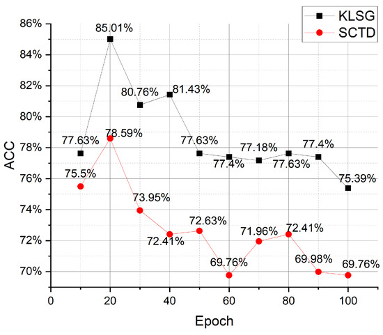
Since the classification models have been pre-trained, a large transfer training epoch may cause the model to overfit on the new data—the pseudo sonar image—resulting in poor detection accuracy on the real sonar dataset. Therefore, it is important to set properly the transfer training epoch. In order to obtain appropriate epoch parameters, we set different epochs to train the ResNet-34 model on the pseudo-sonar image dataset, and then tested the zero-shot classification effect of the ResNet-34 model on the real sonar datasets SCTD and KLSG, as shown in Figure 9. When the training epoch is set to 20, the global accuracy of the zero-shot classification model is higher. Therefore, in the subsequent comparison experiment, the epoch number of transfer training on the pseudo-sonar image is set to 20.

Figure 9. Testing the detection global accuracy of the ResNet-34 model trained with pseudo-sonar images and different epochs on the SCTD and KLSG real sonar datasets.

After the zero-shot classification models are trained on the pseudo-sonar images, we evaluate the classification effect of models on the real sonar dataset. The evaluated metrics include global accuracy (the classification accuracy of all real sonar samples) and average accuracy (the average classification accuracy of real sonar images in each class). The zero-shot classification results are shown in Table 6. On the KLSG dataset, the global accuracies of zero-shot classification models (e.g., ResNet-34, ResNet-152, VGG-19, DenseNet-121, AlexNet, GoogleNet, SqueezeNet, MobileNetV2) trained based on the IDR-ZSL generated images are 82.10%, 44.96%, 28.41%, 55.26%, 44.52%, 80.98%, 49.22%, and 33.33% higher than those of reconstructed image trained models, respectively. The global accuracy of the GoogleNet model trained based on the IDR-ZSL reconstructed ${\tilde{X}}_{cr}$ image can reach 87.92%, and the average accuracy can reach 72.01%. This demonstrates that the proposed IDR-ZSL method can generate the pseudo-sonar images with improved quality, assisting the underwater sonar target classifier in maintaining higher classification accuracy on unseen classes. On the SCTD dataset, the global accuracies of zero-shot classification models (e.g., ResNet-34, ResNet-152, VGG-19, DenseNet-121, AlexNet, GoogleNet, SqueezeNet, MobileNetV2) trained based on the IDR-ZSL generated images are 76.38%, 44.82%, 41.28%, 48.78%, 47.47%, 79.25%, 29.36%, and 24.06% higher than those of reconstructed image trained models, respectively. The global accuracy of the GoogleNet model trained based on the IDR-ZSL reconstructed ${\tilde{X}}_{cr}$ image can reach 83.22%, and the average accuracy can reach 66.55%. The aforementioned results demonstrate that the ${\tilde{X}}_{cr}$ reconstructed by IDR can enhance the performance of the underwater zero-shot classification model in unseen classes.

Table 6. Comparison of zero-shot classification accuracy of different models.

Dataset	Model	Global Accuracy		Average Accuracy
		No Reconstruction	IDR-ZSL	No Reconstruction	IDR-ZSL
KLSG	ResNet-34	2.91%	85.01%	7.78%	63.56%
	ResNet-152	29.98%	74.94%	26.20%	63.13%
	VGG-19	41.39%	69.80%	30.12%	60.14%
	DenseNet-121	20.58%	75.84%	16.68%	62.97%
	AlexNet	33.78%	78.30%	20.29%	57.63%
	GoogleNet	6.94%	87.92%	11.47%	72.01%
	SqueezeNet	30.87%	80.09%	18.60%	60.03%
	MobileNetV2	48.55%	81.88%	35.62%	63.09%
SCTD	ResNet-34	2.21%	78.59%	3.88%	59.06%
	ResNet-152	30.24%	75.06%	20.54%	60.20%
	VGG-19	31.13%	72.41%	24.02%	58.13%
	DenseNet-121	19.87%	68.65%	14.07%	52.45%
	AlexNet	21.85%	69.32%	13.64%	51.61%
	GoogleNet	3.97%	83.22%	5.82%	66.55%
	SqueezeNet	38.63%	67.99%	24.10%	49.53%
	MobileNetV2	47.24%	71.30%	29.89%	51.18%

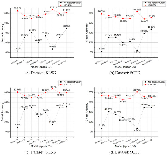
The global accuracy curve of the zero-shot classifiers in KLSG and SCTD datasets are shown in Figure 10. According to Figure 10a,b, the global accuracy of the zero-shot classification models with the IDR method on KLSG dataset except ResNet-152 and VGG-19 is higher than that on SCTD dataset. In addition, the global accuracy of the zero-shot classification models with no reconstruction method is higher on the KLSG dataset than on the SCTD dataset, except for the ResNet-152 and SqueezeNet models. In addition, IDR can effectively improve the detection accuracy of the zero-shot classifier in unseen categories compared with the non-reconstruction method, no matter on KLSG or SCTD datasets. Figure 10c,d give the results of accuracy evaluation for the classifiers trained with 30 epochs. Specifically, the comparison of Figure 10a,c indicates that with the increase of training epoch, the global accuracy of all models with the IDR on the KLSG dataset decreases except for the VGG-19 and AlexNet models. This may be because the models have been pre-trained on a larger dataset, so the transfer training epoch increase is prone to overfitting on the new data. However, we found an interesting phenomenon that the accuracy of the classification model based on no reconstruction method improved significantly with the increase of epoch; notably, the accuracy of ResNet-152 and SqueezeNet models increased by 16.11% and 17.9%, respectively. Furthermore, the comparison of Figure 10b,d indicates that with the increase of training epoch, the global accuracy of all models with the IDR on the SCTD dataset decreases except for the SqueezeNet model.

Figure 10. Comparison of global accuracy fluctuations of different classification models on KLSG and SCTD datasets.

5. Discussion

This work applies to situations where there are no available data of category-specific underwater sonar images, data augmentation methods are difficult to apply to train intelligent models and classify such sonar targets. The proposed IDR-ZSL can synthesize pseudo-sonar images similar to the unseen classes, and help the intelligent zero-shot classification model carry out targeted and effective training, which can transfer the learned knowledge to unseen classes and improve its prediction ability for unseen sonar images. We have conducted a comprehensive test and analyzed the performance of IDR-ZSL: (a) In the image disentanglement reconstruction section, the reconstructed images are almost consistent with the original images; only some categories have slight differences in texture and structure. (b) Regarding the effect of pseudo-sonar image generation, such generation can maintain the structure of the optical content image well and capture the texture of the reference sonar image. Furthermore, we evaluated the function and significance of the $D_{co1}$, $D_{co2}$, and $D_{real}$ networks by ablation study. (c) As for the quantitative evaluation of the pseudo-sonar image quality, we used the IS, FID, and KID metrics, and the results showed that the pseudo-sonar image quality generated by our method had good performance compared with the reference model. For example, the IS and FID value of the pseudo-sonar image of the ship category can reach 4.9114 and 170.4028, respectively, and the KID value of the aircraft category can reach 0.1246. (d) For zero-shot classification performance evaluation, we selected the pre-trained models ResNet-34, ResNet-152, VGG-19, DenseNet-121, AlexNet, GoogleNet, SqueezeNet, and MobileNetV2 for transfer training on the generated pseudo-sonar image samples. After the training, the zero-shot classification performance was tested on real sonar datasets. For example, the accuracy of the GoogNet model reached 87.92% on the KLSG dataset; the accuracy of the GoogNet model reached 83.22% on the SCTD dataset.

Regarding the limitations of this work, the IDR-ZSL zero-shot training requires pseudo-sonar images that are similar to the unseen classes. If the relevant open remote sensing dataset has no samples with similar content to the unseen classes, it is necessary to make a dataset, which takes a long time and incurs costs. In future work, we will introduce 3D printing and other methods to obtain the content images required for the reconstruction of the pseudo-sonar images, and we will be committed to improving the usability of IDR-ZSL.

6. Conclusions

In this work, we design an underwater sonar image classification method based on image disentanglement reconstruction and zero-shot learning, namely, IDR-ZSL. This method can effectively disentangle the image structure and texture vectors of samples based on the encoder network, and then generate pseudo-sonar images by combining the structure vectors of the optical images and the texture vectors of real sonar images. Furthermore, the generated pseudo-sonar images are utilized to train a zero-shot classifier for sonar targets. After training, the zero-shot classifier can predict the sonar samples of unseen classes. Experimental results demonstrate that the proposed method can generate high-quality pseudo-sonar images, improving the zero-shot classifier’s prediction performance.

References

- Xi, Z.; Zhao, J.; Zhu, W. Side-Scan Sonar Image Simulation Considering Imaging Mechanism and Marine Environment for Zero-Shot Shipwreck Detection. IEEE Trans. Geosci. Remote Sens. 2023, 61, 4209713. [Google Scholar] [CrossRef] [Scilit]
- Jones, R.E.; Griffin, R.A.; Unsworth, R.K. Adaptive Resolution Imaging Sonar (ARIS) as a tool for marine fish identification. Fish. Res. 2021, 243, 106092. [Google Scholar] [CrossRef] [Scilit]
- Ødegård, Ø.; Hansen, R.E.; Singh, H.; Maarleveld, T.J. Archaeological use of Synthetic Aperture Sonar on deepwater wreck sites in Skagerrak. J. Archaeol. Sci. 2018, 89, 1–13. [Google Scholar] [CrossRef] [Scilit]
- Steiniger, Y.; Kraus, D.; Meisen, T. Survey on Deep Learning Based Computer Vision for Sonar Imagery. Eng. Appl. Artif. Intell. 2022, 114, 105157. [Google Scholar] [CrossRef] [Scilit]
- Doan, V.S.; Huynh-The, T.; Kim, D.S. Underwater Acoustic Target Classification Based on Dense Convolutional Neural Network. IEEE Geosci. Remote Sens. Lett. 2022, 19, 1500905. [Google Scholar] [CrossRef] [Scilit]
- Kong, W.; Hong, J.; Jia, M.; Yao, J.; Cong, W.; Hu, H.; Zhang, H. YOLOv3-DPFIN: A Dual-Path Feature Fusion Neural Network for Robust Real-Time Sonar Target Detection. IEEE Sens. J. 2020, 20, 3745–3756. [Google Scholar] [CrossRef] [Scilit]
- Srivastava, N.; Hinton, G.; Krizhevsky, A.; Sutskever, I.; Salakhutdinov, R. Dropout: A Simple Way to Prevent Neural Networks from Overfitting. J. Mach. Learn. Res. 2014, 15, 1929–1958. [Google Scholar]
- Shorten, C.; Khoshgoftaar, T.M. A Survey on Image Data Augmentation for Deep Learning. J. Big Data 2019, 6, 60. [Google Scholar] [CrossRef] [Scilit]
- Huo, G.; Wu, Z.; Li, J. Underwater Object Classification in Sidescan Sonar Images Using Deep Transfer Learning and Semisynthetic Training Data. IEEE Access 2020, 8, 47407–47418. [Google Scholar] [CrossRef] [Scilit]
- Huang, C.; Zhao, J.; Zhang, H.; Yu, Y. Seg2Sonar: A Full-Class Sample Synthesis Method Applied to Underwater Sonar Image Target Detection, Recognition, and Segmentation Tasks. IEEE Trans. Geosci. Remote Sens. 2024, 62, 5909319. [Google Scholar] [CrossRef] [Scilit]
- Zhou, J.; Li, Y.; Qin, H.; Dai, P.; Zhao, Z.; Hu, M. Sonar Image Generation by MFA-CycleGAN for Boosting Underwater Object Detection of AUVs. IEEE J. Ocean Eng. 2024, 49, 905–919. [Google Scholar] [CrossRef] [Scilit]
- Lampert, C.H.; Nickisch, H.; Harmeling, S. Attribute-Based Classification for Zero-Shot Visual Object Categorization. IEEE Trans. Pattern Anal. Mach. Intell. 2014, 36, 453–465. [Google Scholar] [CrossRef] [Scilit] [PubMed]
- Xian, Y.; Lampert, C.H.; Schiele, B.; Akata, Z. Zero-Shot Learning—A Comprehensive Evaluation of the Good, the Bad and the Ugly. IEEE Trans. Pattern Anal. Mach. Intell. 2019, 41, 2251–2265. [Google Scholar] [CrossRef] [Scilit] [PubMed]
- Romera-Paredes, B.; Torr, P.H.S. An Embarrassingly Simple Approach to Zero-Shot Learning. In Proceedings of the 32nd International Conference on Machine Learning, ICML Lille, France, 6–11 July 2015; Feris, R.S., Lampert, C., Parikh, D., Eds.; Volume 3, pp. 11–30. [Google Scholar] [CrossRef] [Scilit]
- Socher, R.; Ganjoo, M.; Manning, C.D.; Ng, A.Y. Zero-Shot Learning through Cross-Modal Transfer. In Proceedings of the Advances in Neural Information Processing Systems, Lake Tahoe, NV, USA, 5–8 December 2013. [Google Scholar]
- Han, Z.; Fu, Z.; Chen, S.; Yang, J. Contrastive Embedding for Generalized Zero-Shot Learning. In Proceedings of the 2021 IEEE/CVF Conference on Computer Vision and Pattern Recognition (CVPR), Nashville, TN, USA, 20–25 June 2021; pp. 2371–2381. [Google Scholar] [CrossRef] [Scilit]
- Preciado-Grijalva, A.; Wehbe, B.; Firvida, M.B.; Valdenegro-Toro, M. Self-Supervised Learning for Sonar Image Classification. In Proceedings of the 2022 IEEE/CVF Conference on Computer Vision and Pattern Recognition Workshops (CVPRW), New Orleans, LA, USA, 19–20 June 2022; pp. 1498–1507. [Google Scholar] [CrossRef] [Scilit]
- Gerg, I.D.; Monga, V. Structural Prior Driven Regularized Deep Learning for Sonar Image Classification. IEEE Trans. Geosci. Remote Sens. 2022, 60, 4200416. [Google Scholar] [CrossRef] [Scilit]
- Wang, X.; Jiao, J.; Yin, J.; Zhao, W.; Han, X.; Sun, B. Underwater Sonar Image Classification Using Adaptive Weights Convolutional Neural Network. Appl. Acoust. 2019, 146, 145–154. [Google Scholar] [CrossRef] [Scilit]
- Yang, Z.; Zhao, J.; Yu, Y.; Huang, C. A Sample Augmentation Method for Side-Scan Sonar Full-Class Images That Can Be Used for Detection and Segmentation. IEEE Trans. Geosci. Remote Sens. 2024, 62, 5908111. [Google Scholar] [CrossRef] [Scilit]
- Huang, C.; Zhao, J.; Yu, Y.; Zhang, H. Comprehensive Sample Augmentation by Fully Considering SSS Imaging Mechanism and Environment for Shipwreck Detection Under Zero Real Samples. IEEE Trans. Geosci. Remote Sens. 2022, 60, 5906814. [Google Scholar] [CrossRef] [Scilit]
- Chen, S.; Hou, W.; Khan, S.; Khan, F.S. Progressive Semantic-Guided Vision Transformer for Zero-Shot Learning. In Proceedings of the 2024 IEEE/CVF Conference on Computer Vision and Pattern Recognition (CVPR), Seattle, WA, USA, 16–22 June 2024; pp. 23964–23974. [Google Scholar] [CrossRef] [Scilit]
- Li, Y.; Luo, Y.; Wang, Z.; Du, B. Improving Generalized Zero-Shot Learning by Exploring the Diverse Semantics from External Class Names. In Proceedings of the 2024 IEEE/CVF Conference on Computer Vision and Pattern Recognition (CVPR), Seattle, WA, USA, 16–22 June 2024; pp. 23344–23353. [Google Scholar] [CrossRef] [Scilit]
- Hou, W.; Chen, S.; Chen, S.; Hong, Z.; Wang, Y.; Feng, X.; Khan, S.; Khan, F.S.; You, X. Visual-Augmented Dynamic Semantic Prototype for Generative Zero-Shot Learning. In Proceedings of the 2024 IEEE/CVF Conference on Computer Vision and Pattern Recognition (CVPR), Seattle, WA, USA, 16–22 June 2024; pp. 23627–23637. [Google Scholar] [CrossRef] [Scilit]
- Li, C.; Ye, X.; Cao, D.; Hou, J.; Yang, H. Zero Shot Objects Classification Method of Side Scan Sonar Image Based on Synthesis of Pseudo Samples. Appl. Acoust. 2021, 173, 107691. [Google Scholar] [CrossRef] [Scilit]
- Liu, X.; Ma, Z.; Ma, J.; Zhang, J.; Schaefer, G.; Fang, H. Image Disentanglement Autoencoder for Steganography without Embedding. In Proceedings of the 2022 IEEE/CVF Conference on Computer Vision and Pattern Recognition (CVPR), New Orleans, LA, USA, 18–24 June 2022; pp. 2293–2302. [Google Scholar] [CrossRef] [Scilit]
- Karras, T.; Laine, S.; Aittala, M.; Hellsten, J.; Lehtinen, J.; Aila, T. Analyzing and Improving the Image Quality of StyleGAN. arXiv 2020, arXiv:1912.04958. [Google Scholar]
- Park, T.; Zhu, J.Y.; Wang, O.; Lu, J.; Shechtman, E.; Efros, A.A.; Zhang, R. Swapping Autoencoder for Deep Image Manipulation. Adv. Neural Inf. Process. Syst. 2020, 33, 7198–7211. [Google Scholar]
- Li, K.; Wan, G.; Cheng, G.; Meng, L.; Han, J. Object Detection in Optical Remote Sensing Images: A Survey and a New Benchmark. ISPRS J. Photogramm. Remote Sens. 2020, 159, 296–307. [Google Scholar] [CrossRef] [Scilit]
- Zhang, P.; Tang, J.; Zhong, H.; Ning, M.; Liu, D.; Wu, K. Self-Trained Target Detection of Radar and Sonar Images Using Automatic Deep Learning. IEEE Trans. Geosci. Remote Sens. 2022, 60, 4701914. [Google Scholar] [CrossRef] [Scilit]
- Salimans, T.; Goodfellow, I.; Zaremba, W.; Cheung, V.; Radford, A.; Chen, X. Improved Techniques for Training GANs. arXiv 2016, arXiv:1606.03498. [Google Scholar]
- Heusel, M.; Ramsauer, H.; Unterthiner, T.; Nessler, B.; Hochreiter, S. GANs Trained by a Two Time-Scale Update Rule Converge to a Local Nash Equilibrium. arXiv 2018, arXiv:1706.08500. [Google Scholar]
- Bińkowski, M.; Sutherland, D.J.; Arbel, M.; Gretton, A. Demystifying MMD GANs, arXiv 2021. arXiv:1801.01401. [CrossRef] [Scilit]
- He, K.; Zhang, X.; Ren, S.; Sun, J. Deep Residual Learning for Image Recognition. In Proceedings of the 2016 IEEE Conference on Computer Vision and Pattern Recognition (CVPR), Las Vegas, NV, USA, 27–30 June 2016; pp. 770–778. [Google Scholar] [CrossRef] [Scilit]
- Simonyan, K.; Zisserman, A. Very Deep Convolutional Networks for Large-Scale Image Recognition. In Proceedings of the 3rd International Conference on Learning Representations, ICLR 2015—Conference Track Proceedings, San Diego, CA, USA, 7–9 May 2015; pp. 1–14. [Google Scholar]
- Huang, G.; Liu, Z.; Van Der Maaten, L.; Weinberger, K.Q. Densely Connected Convolutional Networks. In Proceedings of the 2017 IEEE Conference on Computer Vision and Pattern Recognition (CVPR), Honolulu, HI, USA, 21–26 July 2017; pp. 2261–2269. [Google Scholar] [CrossRef] [Scilit]
- Krizhevsky, A.; Sutskever, I.; Hinton, G. ImageNet Classification with Deep Convolutional Neural Networks. In Proceedings of the Advances in Neural Information Processing Systems 25 (NIPS 2012), Lake Tahoe, NV, USA, 3–6 December 2012. [Google Scholar] [CrossRef] [Scilit]
- Szegedy, C.; Liu, W.; Jia, Y.; Sermanet, P.; Reed, S.; Anguelov, D.; Erhan, D.; Vanhoucke, V.; Rabinovich, A. Going Deeper with Convolutions. In Proceedings of the 2015 IEEE Conference on Computer Vision and Pattern Recognition (CVPR), Boston, MA, USA, 7–12 June 2015; pp. 1–9. [Google Scholar] [CrossRef] [Scilit]
- Iandola, F.N.; Han, S.; Moskewicz, M.W.; Ashraf, K.; Dally, W.J.; Keutzer, K. SqueezeNet: AlexNet-level Accuracy with 50x Fewer Parameters and <0.5 MB Model Size. arXiv 2016, arXiv:1602.07360. [Google Scholar]
- Sandler, M.; Howard, A.; Zhu, M.; Zhmoginov, A.; Chen, L.C. MobileNetV2: Inverted Residuals and Linear Bottlenecks. In Proceedings of the 2018 IEEE/CVF Conference on Computer Vision and Pattern Recognition, Salt Lake City, UT, USA, 18–23 June 2018; pp. 4510–4520. [Google Scholar] [CrossRef] [Scilit]
Disclaimer/Publisher’s Note: The statements, opinions and data contained in all publications are solely those of the individual author(s) and contributor(s) and not of MDPI and/or the editor(s). MDPI and/or the editor(s) disclaim responsibility for any injury to people or property resulting from any ideas, methods, instructions or products referred to in the content. |
© 2025 by the authors. Licensee MDPI, Basel, Switzerland. This article is an open access article distributed under the terms and conditions of the Creative Commons Attribution (CC BY) license (https://creativecommons.org/licenses/by/4.0/).