Article

Climate Impact on Evapotranspiration in the Yellow River Basin: Interpretable Forecasting with Advanced Time Series Models and Explainable AI

by
Sheheryar Khan
1,
Huiliang Wang
1,*,
Umer Nauman
2,
Rabia Dars
1,3,
Muhammad Waseem Boota
4 and
Zening Wu
1
1
School of Water Conservancy and Transportation, Zhengzhou University, Zhengzhou 450001, China
2
College of Information Science and Engineering, Henan University of Technology, Zhengzhou 450001, China
3
Geothermal and Ecological Geology Research Centre, Zhengzhou University, Zhengzhou 450001, China
4
College of Geography and Environmental Science, Henan University, Kaifeng 475004, China
*
Author to whom correspondence should be addressed.
Remote Sens. 2025, 17(1), 115; https://doi.org/10.3390/rs17010115
Submission received: 10 December 2024 / Accepted: 27 December 2024 / Published: 1 January 2025
(This article belongs to the Special Issue Advanced Techniques for Water-Related Remote Sensing (Second Edition))

Abstract

:
Evapotranspiration (ET) plays a crucial role in the hydrological cycle, significantly impacting agricultural productivity and water resource management, particularly in water-scarce areas. This study explores the effects of key climate variables temperature, precipitation, solar radiation, wind speed, and humidity on ET from 2000 to 2020, with forecasts extended to 2030. Advanced data preprocessing techniques, including Yeo-Johnson and Box-Cox transformations, Savitzky–Golay smoothing, and outlier elimination, were applied to improve data quality. Datasets from MODIS, TRMM, GLDAS, and ERA5 were utilized to enhance model accuracy. The predictive performance of various time series forecasting models, including Prophet, SARIMA, STL + ARIMA, TBATS, ARIMAX, and ETS, was systematically evaluated. This study also introduces novel algorithms for Explainable AI (XAI) and SHAP (SHapley Additive exPlanations), enhancing the interpretability of model predictions and improving understanding of how climate variables affect ET. This comprehensive methodology not only accurately forecasts ET but also offers a transparent approach to understanding climatic effects on ET. The results indicate that Prophet and ETS models demonstrate superior prediction accuracy compared to other models. The ETS model achieved the lowest Mean Absolute Error (MAE) values of 0.60 for precipitation, 0.51 for wind speed, and 0.48 for solar radiation. Prophet excelled with the lowest Root Mean Squared Error (RMSE) values of 0.62 for solar radiation, 0.67 for wind speed, and 0.74 for precipitation. SHAP analysis indicates that temperature has the strongest impact on ET predictions, with SHAP values ranging from −1.5 to 1.0, followed by wind speed (−0.75 to 0.75) and solar radiation (−0.5 to 0.5).

1. Introduction

Evapotranspiration (ET) is a critical component of the hydrological cycle, as it combines the processes of water evaporation from soil and other surfaces and transpiration from plants. ET has a direct impact on agricultural productivity, water resource management, and climate modeling, notably in regions that are susceptible to water scarcity, such as the Yellow River Basin China (YRBC), as a critical component in the water balance equation [1]. Often referred to as the “cradle of Chinese civilization”, the YRBC holds immense agricultural significance. However, climate variability and fluctuating water availability pose substantial challenges [2]. Therefore, it is of the utmost significance to accurately predict ET in this region to guarantee sustainable agricultural planning and water resource management.
In the past, empirical models or basic regression techniques were the primary methods of ET forecasting. However, these methods, while useful, frequently lack the sophistication necessary to capture the intricate interactions between climate variables and ET [3]. In recent years, the emergence of advanced time series models has equipped researchers with more comprehensive tools to accurately predict ET [4]. Models such as Prophet, the Exponential Smoothing State Space Model (ETS), and the Seasonal Autoregressive Integrated Moving Average (SARIMA) have successfully modeled time series data that exhibit seasonal patterns and trends [5,6]. In previous research, descriptive methods and time series models, including SARIMA and ETS, have been employed to conduct a comprehensive analysis of ET trends and their variability in the YRBC. However, these methods frequently failed to provide a clear understanding of the impact of critical climate variables (Table 1). A valid solution to bridge this gap is provided by recent advancements in Explainable AI (XAI) techniques, such as SHapley Additive Explanations (SHAPs), which enable interpretable ET forecasting. Nevertheless, these models frequently function as “black boxes”, which means that they provide precise predictions but lack transparency in disclosing how input variables affect the output. For example, although models such as SARIMA or ETS can accurately predict ET, they fail to elucidate the specific contributions or interactions of climatic variables such as temperature or precipitation, which complicates the comprehension or validation of the causal relationships that underlie the predictions. This lack of interpretability is a substantial limitation, particularly in the context of environmental science, where the comprehension of the causal relationships between variables is essential for informed decision-making [7]. To address this challenge, the discipline of XAI has emerged, providing techniques that improve machine learning models’ transparency by elucidating the contributions of individual input variables to the model’s predictions [8]. SHAP has become increasingly popular among these techniques as a result of its consistent and interpretable explanations and its strong theoretical foundation in cooperative game theory [8]. Recent studies indicate that XAI approaches are offering significant insights into the decision-making procedures of models employed in climate and meteorology, hence enhancing trust in their forecasts [9,10]. Mamalakis et al. [9] examined the effective application of XAI in meteorology and climate science, providing substantial insights into model decision-making for climate forecasting. Chakraborty et al. [10] highlight the application of XAI to assess the effects of climate change on energy consumption, illustrating the efficacy of XAI in delivering clear and actionable insights for decision-makers across various climate scenarios. This study investigates the potential of integrating XAI techniques with advanced time series models to improve the interpretability of ET forecasting in the YRBC. The study aims to evaluate the predictive capabilities of these models such as SARIMA, Prophet, STL + ARIMA, TBATS, ARIMAX, and ETS. Additionally, the study utilizes SHAP values to provide a transparent explanation of the impact of key climate variables temperature, precipitation, solar radiation, wind speed, and humidity on ET predictions. The integration of SHAP values not only enables a more profound understanding of the models’ behavior but also offers valuable insights into the relative significance of each climate variable in influencing ET variability in the region. Our research is based on prior studies that have emphasized the critical role of ET in the YRBC and the necessity of precise forecasting to effectively manage water resources [1,2]. This research introduces innovative XAI algorithms, specifically SHAP, to improve the interpretability of ET forecasting models. This approach offers transparent and extensive insights into the influence of certain climate variables on ET projections, beyond traditional “black-box” methodologies. The integration of advanced time series models with XAI approaches enhances forecast precision and enriches comprehension of the fundamental connections between climatic variables and ET. This combined emphasis on interpretability and accuracy signifies a notable progression in climate modeling, providing meaningful insights for water resource management and sustainable planning in the YRBC and beyond.

2. Study Area and Data

2.1. Study Area

The YRBC, situated in northern China, is a critical hydrological system that is frequently referred to as the “center of Chinese civilization” due to its historical importance Figure 1 [13]. The basin, which encompasses nine provinces, including Qinghai, Sichuan, Gansu, Ningxia, Inner Mongolia, Shaanxi, Shanxi, Henan, and Shandong, and covers an area of approximately 795,000 square kilometers, is home to a population of over 150 million individuals [14]. The basin’s hydrological dynamics are intricately defined by its distinct upper, middle, and lower reaches, each of which possesses distinctive geological and climatic characteristics. The Tibetan Plateau is the source of the cold arid conditions that characterize the upper reaches, primarily sustained by glacial meltwater and precipitation [15]. The river’s high sediment burden, which is the highest of any river globally and has historically caused significant flooding issues, is primarily due to the presence of steep valleys and loess plateaus in the middle reaches [16]. The lower reaches of the river traverse the North China Plain, a critical agricultural region subject to significant water demand due to intensive farming practices [17]. The YRBC is indispensable to China’s agricultural sector, as it supplies water to irrigate nearly 13% of the country’s arable land [18]. However, the region is confronted with significant environmental challenges, such as water scarcity, pollution, and ecological degradation, which are the result of the rapid expansion of agricultural activities, urbanization, and industrialization [19]. These issues are further exacerbated by climate change, which alters precipitation patterns, increases the frequency and intensity of droughts, and affects the availability of water resources [20,21,22].

2.2. Data Collection

The YRBC, a critical hydrological system in northern China, has been the subject of extensive research for a long time. This is due to its critical role in supporting agriculture, water resource management, and the maintenance of large populations. This study utilizes a comprehensive collection of datasets that extend from 2001 to 2020 due to limited availability to gain a more comprehensive understanding of the dynamics of ET and its interaction with critical climatic variables. The dataset was used for both calibration and model evaluation purposes to ensure model robustness. Together, the datasets include MODIS Global Terrestrial ET (MOD16A2), TRMM estimates of precipitation (3B42), GLDAS-2.1 data on solar radiation and humidity, MODIS Land Surface Temperature/Emissivity (MOD11A2), and ERA5 daily wind speed data showed in Table 2 [23,24]. Integrated datasets enable a robust investigation of ET, which is affected by complicated interactions between temperature, precipitation, solar radiation, wind speed, and humidity [25]. The MODIS ET product (MOD16A2) is essential for monitoring terrestrial water vapor flow, while the TRMM and ERA5 datasets provide precipitation and wind dynamics insights. These climatic determinants are crucial to understanding regional water balance and how climate variability affects agricultural productivity and water resource sustainability in the basin [26,27]. The study employs an innovative approach that applies advanced time series models enhanced by XAI techniques to improve the models’ interpretability. This framework for research not only makes ET predictions more accurate but it also gives us a better picture of how each climate variable works [12,28,29].

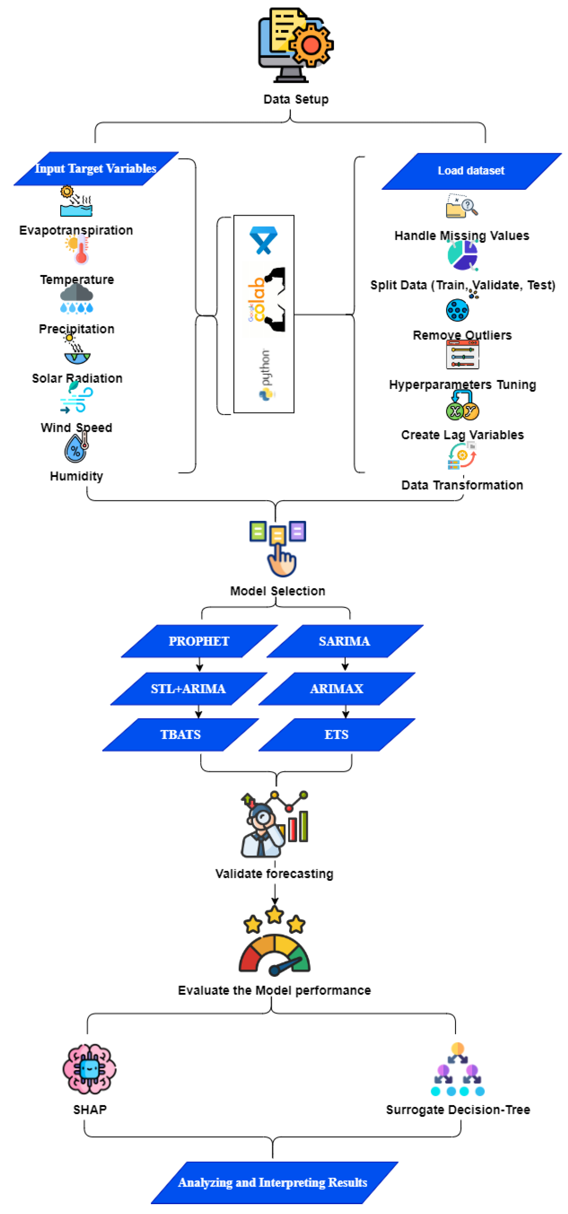
2.3. Data Preprocessing

The climate data in YRBC poses distinct problems for ET modeling, characterized by skewed distributions, significant fluctuation, and extreme outliers resulting from the region’s climatic trends. To tackle these problems and improve model reliability, we implemented a range of customized preprocessing techniques. Each technique was selected to correspond with the distributional and variability attributes of the climate variables, as outlined in Table 3. The Yeo-Johnson transformation was selected to rectify these difficulties by modifying skewness while accommodating zeros in the dataset [30]. Savitzky–Golay smoothing succeeds in this, enhancing data quality without distorting the original structure through noise reduction and trend preservation [31]. The Box-Cox transformation normalizes skewed precipitation data in the YRBC. Figure 2 shows that the transformation reduces skewness (0.221) and improves symmetry, creating a more normal-like distribution with kurtosis (−0.2491) [32]. Following the application of the Box-Cox transformation to precipitation and UV data, we assessed normality by computing skewness and kurtosis. A skewness number near 0 and a kurtosis close to 3 would signify the normality [33]. Temperature data contain sporadic extremely low values and zeros, which impact normalcy and data stability. The Yeo-Johnson transformation was utilized to stabilize variance and address skewness, accommodating zero values, while severe outliers were eliminated to mitigate bias. Solar radiation in the YRBC can vary considerably, particularly during seasonal transitions. The Box-Cox transformation in Figure 2 reduces the skewness (−0.1650) and slightly flattens the tails (kurtosis: −0.2188), achieving a closer-to-normal distribution of solar radiation. The wind speed data in the YRBC demonstrate significant variability. Z-score standardization was utilized to normalize the data for comparability, while exponential smoothing was implemented to identify patterns and mitigate short-term variations, hence improving modeling consistency. Humidity data frequently exhibit considerable skewness and variability, potentially impacting model stability. A logarithmic and quantile transformation was utilized to rectify skewness and constrain extreme values, hence ensuring compliance with model assumptions. To generate a dataset that is more uniform and stable, advanced refining methods are implemented. These preprocessing procedures guarantee that the dataset adheres to the assumptions of the chosen time series models, including normality and variance stability, hence augmenting model robustness and prediction reliability [34,35]. The resulting error indicators (MAE, MSE, and RMSE) are dimensionless, as they reflect the performance of variables on a standardized scale, as ET and climate data are normalized.
The study uses the Yeo-Johnson Transformation Equation (1) to address skewness and manage zero/negative values in ET and temperature data. Where y is original data values, y t r a n s f o r m e d is the transformed data value, and γ represents the transformation parameter, which adjusts the skewness [30].
y t r a n s f o r m e d = y + 1 γ 1 γ ln y + 1 , γ 0 , γ = 0
The Box-Cox Transformation Equation (2) normalizes precipitation and ultraviolet (UV) observations. Where y is original data values, y t r a n s f o r m e d is transformed data values, and γ represents the transformation parameter, which controls the transformation strength for normalizing data [32].
y t r a n s f o r m e d = y γ 1 γ ln y , γ 0 , γ = 0
The study utilized Equation (3) of the Savitzky–Golay smoothing method to minimize noise and preserve the integrity of the data trends [31]. In Equation (3), y i + k shows the original data point at position i where k indexed with the smoothing window and c k coefficient of the polynomial. y s m o o t h e d i is the smoothed data point at position i and m represents the size of the window.
y s m o o t h e d i = k = m m c k . y i + k
The coefficients of a polynomial applied to the data inside an aperture of size 2m + 1 are represented by c and k in Equation (3). The Z-score standardization is used in Equation (4) to normalize wind speed data used in the study where x represents original data, μ is the mean, and σ is the standard deviation of the data [36]. Z-score standardization was employed to modify the dataset’s mean to zero and variance to one, enhancing comparability among variables with disparate scales. This contrasts with normalization, which suggests a modification to conform to statistical distributions.
z = x μ σ
where μ represents the mean and σ represents the standard deviation of the data. The logarithmic and quantile transformations in Equation (5) applied to reduce the skewness. Where y l o g represents the log-transformed, y q u a n t i l e denotes the quantile transformed, and function F(y) represents the empirical cumulative distribution function of the data [37]. To prevent anomalies from distorting the data, the study used quantile-based approaches to exclude extreme deviations in wind speed and moisture.
y l o g = l o g y , y q u a n t i l e = F 1 F y

3. Methodology

This work focuses on integrating advanced time series forecasting models with XAI methodologies to enhance the accuracy and interpretability of ET forecasting in the YRBC.
The research methodology, depicted in Figure 3, methodically predicts ET, utilizing multiple climatic factors, such as temperature, precipitation, solar radiation, wind speed, and humidity. The methodology begins with data preprocessing, which includes missing value imputation, outlier elimination, and the construction of lag variables, then followed by data partitioning into training and testing sets, with 70% of the data (2000–2015) used for training and 30% (2016–2020) reserved for testing. A distinct calibration period was not employed because of the extensive preparation methods and the restricted historical data accessible. This method sought to enhance model training while utilizing available data to ensure reliable predictions. Various time series models, Prophet, SARIMA, STL + ARIMA, ARIMAX, TBATS, and ETS, are subsequently chosen and assessed utilizing performance criteria including MAE, MSE, and RMSE. This methodology uniquely integrates SHAP and XAI algorithms to quantitatively assess the influence of each climate variable on model predictions while employing a Surrogate Decision-Tree model to visually elucidate complex model behaviors, thereby improving transparency and interpretability. This thorough methodology guarantees precise ET forecasting while offering an enhanced understanding of the model’s decision-making process and the impact of climatic variables. The climate variables utilized to model ET are derived from historical data spanning the years 2001 to 2020. These datasets, derived from satellite observations and reanalysis models as declared in Table 1, offer recorded and estimated historical circumstances, rather than future predictions. The model was calibrated using historical climate variables, and the subsequent ET forecasts for the 2021–2030 period are derived from the patterns and correlations established in this historical data.

3.1. Advanced Time Series Models

This research used a collection of advanced time series forecasting algorithms. Some models like ARIMAX include external climate variables as exogenous variables, while others like SARIMA, Prophet, and ETS do not incorporate the exogenous variables.
SARIMA: The SARIMA model was selected to identify seasonal patterns in ET and climate data due to its capacity to represent seasonality following differencing. This methodology is most effective with stationary data that displays periodic trends and is ideally suited for time series data with consistent seasonal patterns. The mathematical representation of the model SARIMA is provided in Equation (6). y t is the value of time series at time t , i represents the non-seasonal autoregressive coefficient, θ j denotes the non-seasonal moving average coefficient, l S is the seasonal period length, and t   is the white noise error term [6]. The non-seasonal autoregressive and moving average phases are denoted by p and q, respectively, whereas the seasonal equivalents are denoted by P and Q.
y t = i = 1 p i y t i j = 1 q θ j t j + k = 1 P φ k y t k S + i = 1 Q Θ l t l S + t
ETS: The ETS model was used because of its breakdown into error, trend, and seasonal components, which improves interpretability. ETS is proficient for data exhibiting distinct seasonal and trend patterns, rendering it appropriate for the markedly seasonal ET and climate data in the YRBC. The ETS Model is expressed in Equation (7), where y t is the value of time series at time t , l t 1 represents the level component at time t 1 , b t 1 denotes the trend component at t 1 , s t S is the seasonal component, lagged by S period, and t is the error term at time t [4].
y t = l t 1 + b t 1 . s t S + t
Prophet Model: Prophet is resilient to absent data, anomalies, and seasonal fluctuations, rendering it suitable for environmental datasets characterized by inconsistencies. It facilitates adaptable modeling of seasonality and holidays, advantageous for ET data affected by seasonal climatic fluctuations. The Prophet Model Equation (8) is a method that breaks down time series data into three components: trend, seasonality, and holiday impacts [5,38]. The function y t is the value of time series at time t ,   g t reflects the trend, s t represents the seasonal element, and h t indicates holidays or other external occurrences and t is the error term at time t .
y t = g t + s t + h t + t
TBATS model: The TBATS approach can manage intricate seasonality and is especially appropriate for data exhibiting numerous seasonal cycles. Due to the seasonal variations in ET and climatic conditions in the YRBC, TBATS was incorporated to address these intricacies. The statistical representation of the TBATS model, incorporating seasonality using Fourier terms, is given Equation (9). With the use of Fourier terms, this model can represent complicated seasonality, where y t is the value of time series at time t , λ t 1 is the parameter to handle data with Box-Cox transformation, α t represents an additional parameter used to adjust for irregularities within the seasonal components of the model, j denotes the autoregressive coefficient, and Θ k is the moving average coefficient [4].
y t = λ t 1 y t λ α t + j = 1 p j y t j + k = 1 q Θ k t
STL + ARIMA: This hybrid methodology uses STL decomposition to isolate trend, seasonal, and residual components prior to the application of ARIMA on the residuals, hence offering adaptability for seasonal data. STL+ARIMA is proficient for data exhibiting non-stationary seasonal patterns, facilitating a more customized fit to ET data. The STL combined with ARIMA is shown in Equation (10). The trend, seasonal, and residual components are represented by T, S, and R, respectively [39]. We apply the ARIMA model to the residual component R t .
y t = T t + S t + R t
ARIMAX: The ARIMAX model was chosen to include external climate elements as exogenous variables, rendering it appropriate for simulating the impact of specific climate variables, such as temperature and precipitation, on ET. This paradigm is especially advantageous for linear correlations with external factors. The ARIMAX model, which incorporates exogenous variables such as climate related factors, is described in Equation (11) [40], where Φ i represent the autoregressive, θ j denotes the moving average coefficient, term X t k indicates the exogenous inputs, and γ k represents the coefficient for the exogenous variables.
y t = I = 1 p Φ i y t i + j = 1 q θ j t j + k = 1 r γ k X t k + t

Evaluation Metrics for Models

The research employs three rigorous statistical guidelines to assess the models [41]:
The Mean Absolute Error (MAE) is calculated using Equation (12). Where y i denoted the actual value, y ^ i represents the predicted value, and n is the number of observations.
M A E = 1 n i = 1 n y i y ^ i
Equation (13) illustrates the Mean Squared Error (MSE), where y i denotes the actual value, y ^ i represents the predicted value, and n is the number of observations.
M S E = 1 n i = 1 n y i y ^ i 2
Root Mean Squared Error (RMSE) refers to the following Equation (14), where y i denotes the actual value, y ^ i represents the predicted value, and n is the number of observations.
R M S E = 1 n i = 1 n y i y ^ i 2
Nash–Sutcliffe Efficiency (NSE) is a commonly employed statistic for assessing the congruence between a model’s predictions and actual data [42]. The comparison of the model’s predictions to the mean of the observed data reveals that values approaching one signify superior predictive accuracy. An NSE value of zero indicates that the model’s performance is equivalent to utilizing the mean of the observed data, whereas values below zero denote that the model’s performance is inferior to the mean. This study utilizes the NSE to evaluate the efficacy of several forecasting models in predicting ET.
N S E = 1 i = 1 n y i y ¯ i 2 i = 1 n y i y ^ i 2
where y i in Equation (15) represents the actual observed data at time i while y ^ i is the predicted values from the model at the same time point. The mean of the observed values is denoted as y ¯ i where n represents the total number of data points in the dataset.
Pearson’s correlation coefficient (R) analyzes the relationship between independent and dependent variables, emphasizing its function in identifying multicollinearity [43]. The research examines correlations among independent variables to uncover potential mediating or moderating effects in regression models.
R = i = 1 n y i y ¯ y ^ i y ^ ¯ i = 1 n y i y ¯ i 2 i = 1 n y ^ i y ^ ¯ 2
y i represents the actual observed values, y ^ i represents the predicted values, and y ¯ and y ^ ¯ are the mean of the observed and predicted values, respectively, in Equation (16).

3.2. Elucidate the Techniques of XAI

To improve the comprehensibility of the models, the SHAP method was used. SHAP values convey a glimpse at the individual impact of each climatic parameter on the forecasts generated by the models. Formula for Calculating the SHAP Value Equation (17) [44], where i is the Shapley value for feature i , representing its contribution to the prediction, N is the set of all features, S is the subset of feature not including i , and f ( S ) denotes the model output using subset S .
i = S N \ i S N S 1 N f S i f S
In this context, f(S) refers to the model’s output using a subset of S features, whereas N refers to all features. Equations (1)–(15) are essential for developing a complete and successful framework for ET forecasting with XAI integration. These mathematical equations enhance each phase of the process, from data preparation to model evaluation and outcome interpretation. Data transformation techniques such as Yeo-Johnson, Box-Cox, and Z-Score normalization effectively prepare input data by eliminating noise, rectifying skewness, and mitigating outliers, hence enhancing the stability and dependability of the model’s predictions. The smoothing methods enhance the data, facilitating precise time series analysis by removing superfluous variations. Assessment measures like MAE, MSE, and RMSE examine prediction errors to find the most accurate and resilient forecasting approach. SHAP values clarify the model’s internal mechanics. SHAP gives feature relevance to help stakeholders understand which factors significantly affect model predictions, boosting confidence and responsibility. Using advanced data processing, error reduction, and explainability frameworks creates a durable, consistent, and interpretable forecasting system that accurately predicts fundamental climate changes, where Equations (1)–(15) give a reliable forecasting strategy that balances performance and interpretability, revealing ET trends and their causes.

3.3. Algorithms for Time Series Forecasting with XAI Integration

3.3.1. Algorithm 1: XAI-Based Feature Attribution

Using several time series models, the study aims to estimate ET values for 2021–2030. Additionally, it seeks to improve the interpretability of forecasts by using SHAP values. A description of the algorithm’s process may be found in the following steps:
Preprocessing: These processes differ by data type and they transform and normalize climate variables during preparation. The Yeo-Johnson approach is employed to normalize data distribution and manage negative values, with the transformations applied to ET and temperature. The Box-Cox approach facilitates the transformation of precipitation and solar radiation to stabilize variance and make the data more regular. Z-score normalization normalizes wind speed by zeroing the average and unit-scaling the variability. The humidity data undergo a logarithmic and quantile transformation to mitigate skewness and promote uniformity. Savitzky–Golay smoothing reduces noise in climate variables while preserving major patterns and trends. Quantile techniques are used to outlier the reduction cap or eliminate extreme values, improving modeling accuracy.
Model Selection: The time series models, including SARIMA, ETS, Prophet, TBATS, STL + ARIMA, and ARIMAX, are trained on the filtered dataset. This diversified model selection promotes resilience in predicting by evaluating numerous techniques.
Forecasting: Each model predicts the ET values for the time frame of 2021–2030, producing a variety of projections using various modeling methodologies.
Evaluation: The efficacy of each model is assessed using metrics such as MAE, MSE, and RMSE.
The model with the lowest RMSE is selected for the final forecasts since it offers the optimal trade-off between punishing significant mistakes and preserving accessibility.
Explainability: After selecting the appropriate model, SHAP values are calculated to evaluate the impact of each climatic variable on the forecasts made by the model. SHAP values provide straightforward clarity for the model outcomes by revealing the factors (such as temperature and precipitation) that have the greatest effect on the anticipated ET. The pseudocode for Algorithm 1 is shown below, as follows:
Algorithm 1: Explainable Artificial Intelligence (XAI) Time Series Forecasting.
Input: Climate dataset (D)
Output: Projected ET values for the period 2021–2030, along with corresponding SHAP values.
Preprocessing
  Iterate over each variable Vi in the set D:
    If Vi represents either ET or temperature:
      Utilize the Yeo-Johnson transformation.
    If Vi represents either precipitation or solar radiation:
      Perform the Box-Cox transformation
    If Vi represents wind speed, then use Z-score normalization.
    If Vi represents humidity:
      Utilize logarithmic and quantile transformation techniques.
    Perform Savitzky–Golay smoothing on the variable Vi.
  Apply quantile-based approaches to eliminate outliers from dataset
Selection of model
  Iterate over each model Mi in the set (SARIMA, ETS, Prophet, TBATS, STL + ARIMA, ARIMAX) and do the following steps:
    Adjust the parameters of Mi to the preprocessed dataset D.
Prediction
  Perform the following steps for each model Mi:
    Predicted ET levels for the period of 2021–2030.
Assessment
  Perform the following steps for each model Mi:
    MAE, MSE, and RMSE.
  Choose the model that has the lowest RMSE.
Explainability
  Utilize the SHAP method on the model that has shown the highest level of performance.
  Compute the SHAP values for each feature.
Return
forecasted ET, SHAP values
End Algorithm
This technique combines various time series models with XAI using SHAP, providing precise projections and comprehensive feature allocation. Within the realm of the literature, the primary emphasis in time series forecasting often lies on the evaluation of model performance alone. Nevertheless, the use of XAI methods such as SHAP in this algorithm adds an additional level of interpretability, allowing users to comprehend the rationale behind certain predictions. This feature is especially valuable in domains such as climate science.

3.3.2. Algorithm 2: SHAP-Based Feature Attribution

Algorithm 2 utilizes SHAP to ascertain the significance of features in a time series model, hence offering accessibility and comprehensibility for the predicted ET values. Let us break down each section of the algorithm:
I. Initializing the SHAP Explainer.
Configure the top-performing model’s SHAP explanation. We calculate SHAP values using dataset attributes to understand the model’s prediction process. We input SARIMA, Prophet, or ARIMAX, the algorithm that performed best in Algorithm 1, into the SHAP Explainer. The explanation can separate the model’s results and assign SHAP values to variables like temperature, humidity, and wind speed. Initializing the SHAP explanation is essential to determining how much each feature affects model predictions.
II. Calculate the SHAP values for each data point.
Calculate the SHAP values for every prediction the model generates. For every data point in the dataset, the algorithm executes the model to obtain the estimated ET value. The Equation (18) may be expressed, as follows:
y ´ i = M x i y ´
The equation states that the value of i is determined by function M, which is the model, and the input data xi. We calculate SHAP values for each input feature after the prediction. SHAP values show how temperature, wind speed, and humidity affected the forecast. We maintain the unique contributions of each data point. SHAP values explain how features affect individual predictions rather than generalizing across the dataset. Due to the extensive study, users may see how daily or monthly meteorological variables affect ET forecasting.
III. Accumulate the SHAP values for all data points
To calculate SHAP values for all features in the dataset to assess their importance, data point SHAP values are concatenated after calculation. This phase determines the mean or total SHAP values for each feature to determine its overall contribution to the model’s predictions. The model’s predictions would suffer if the temperature consistently had high SHAP values for all data points. However, a parameter like wind speed with lower SHAP values may be less important for ET forecasting. This information benefits decision-makers because it emphasizes climate elements such as temperature and precipitation, which are essential for ET estimation.
IV. Provide rankings based on SHAP values
To prioritize features by cumulative SHAP values to show which qualities have the biggest impact on model predictions. A SHAP-ordered list of temperature, humidity, and wind speed is the final product. This ranking sorts characteristics by their impact on the model’s predictions, from most to least influential. The rankings provide a clear and concise picture of how climatic factors affect ET estimates. The pseudocode for Algorithm 2 is shown below, as follows:
Algorithm 2: SHAP-based Feature Attribution
Input: (Dataset D), Model (M)
Output: SHAP values for vital features
Initialized SHAP explainer
   S H A P e x p l a i n e r = S H A P M
Determine SHAP values for all records
Perform the following for every xi in D
y ´ = M x i  # Model prediction
     S H A P v a l u e s = S H A P e x p l a i n e r x i  #Compute SHAP values for xi and save the SHAP_values.
Consolidate SHAP values
   S H A P i m p o r t a n c e = S u m   S H A P
Return   S H A P i m p o r t a n c e
End Algorithm
Algorithm 2 uses SHAP as it offers an explicable framework that dissects the model’s choice-making procedure. By computing SHAP values for each prognosis and consolidating them, the technique provides both local (individual prediction-level) and global (total feature significance) insights. Utilizing SHAP enhances user confidence and comprehension of model outcomes, rendering it particularly pertinent in environmental forecasting and other fields necessitating clarity in machine learning approaches.

4. Results

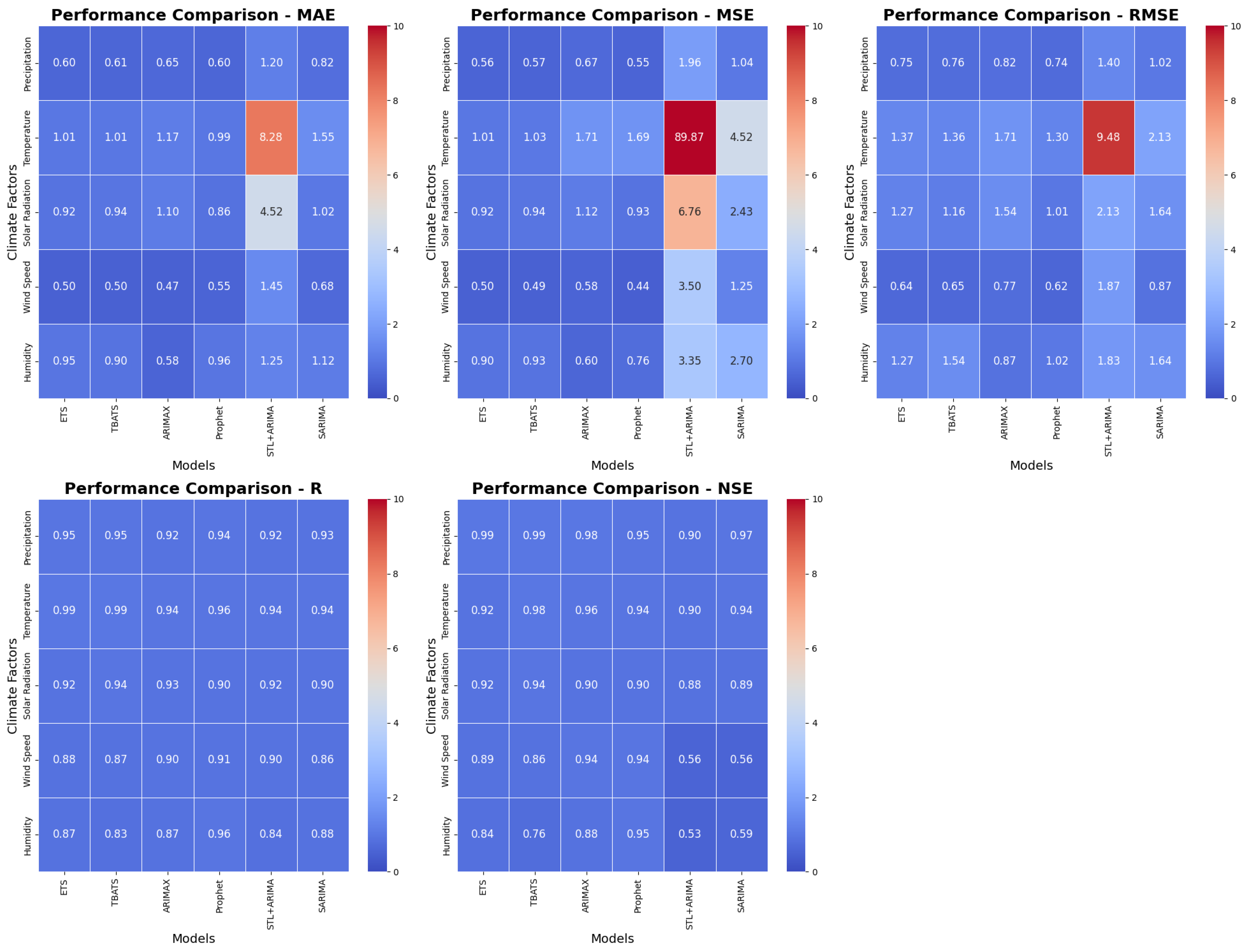
4.1. Overview of Model Performance

This research rigorously evaluated six advanced time series models: ARIMAX, SARIMA, ETS, STL + ARIMA, TBATS, and Prophet, for predicting ET in relation to significant climate factors within the YRBC. The assessment of each model was performed utilizing stringent statistical metrics, including Mean MAE, MSE, RMSE, R, and NSE. The comparative heat maps offer a comprehensive overview of the model’s performance, highlighting distinct trends and underscoring the strengths and weaknesses of each technique across diverse climate factors. The ETS and TBATS models exhibited reliable accuracy across most climate variables. The ETS model attained the minimal MAE values of 0.6 for precipitation and 0.75 for wind speed, as illustrated in Figure 4. The ETS model in R exhibited a high correlation of 0.95 for precipitation and 0.89 for Wind Speed, signifying robust forecast ability in these domains. TBATS demonstrated comparable performance, achieving an MAE of 0.61 for precipitation and 0.57 for temperature, along with R values of 0.95 for precipitation and 0.99 for temperature, further substantiating its efficacy in ET forecasting. TBATS achieved NSE values of 0.72 for precipitation and 0.98 for temperature, indicating its exceptional model efficacy in these instances. The STL + ARIMA model exhibited significant heterogeneity in its performance. The model exhibited a notably elevated MAE of 90 for humidity, indicating that the STL + ARIMA framework may have difficulty encapsulating the intricacies of this variable. The MSE and RMSE metrics similarly illustrate this tendency, with STL + ARIMA exhibiting the greatest error values of 9.5 (MSE) and 3.4 (RMSE) for precipitation and wind speed, respectively. Regarding R, STL + ARIMA demonstrated reduced values for many variables, including 0.91 for precipitation and 0.86 for wind speed; however, the NSE value for precipitation was merely 0.58, signifying a suboptimal fit for this variable. The SARIMA model faced difficulties, especially regarding temperature. SARIMA had moderate accuracy for wind speed with an RMSE of 2.7; however, its performance for temperature was subpar, indicated by an MAE of 1 and an MSE of 2.1. The R-value for temperature was 0.93, showing a moderate correlation, while the NSE for temperature was 0.78, suggesting potential for enhancement. SARIMA exhibited superior performance with wind speed, with R = 0.89 and NSE = 0.68, indicating a satisfactory match for this variable. The ARIMAX model, although generally dependable, exhibited an elevated RMSE of 2.4 for wind speed, indicating possible overfitting or heightened sensitivity to this variable. The R-value for wind speed was 0.87 and the NSE was 0.53, indicating reasonable performance with certain limitations in effectively representing the dynamics of wind speed. The increased error margin for wind speed indicates possible constraints in the ARIMAX model’s capacity to generalize across all climatic variables.

4.2. Model-Specific Performance Analysis

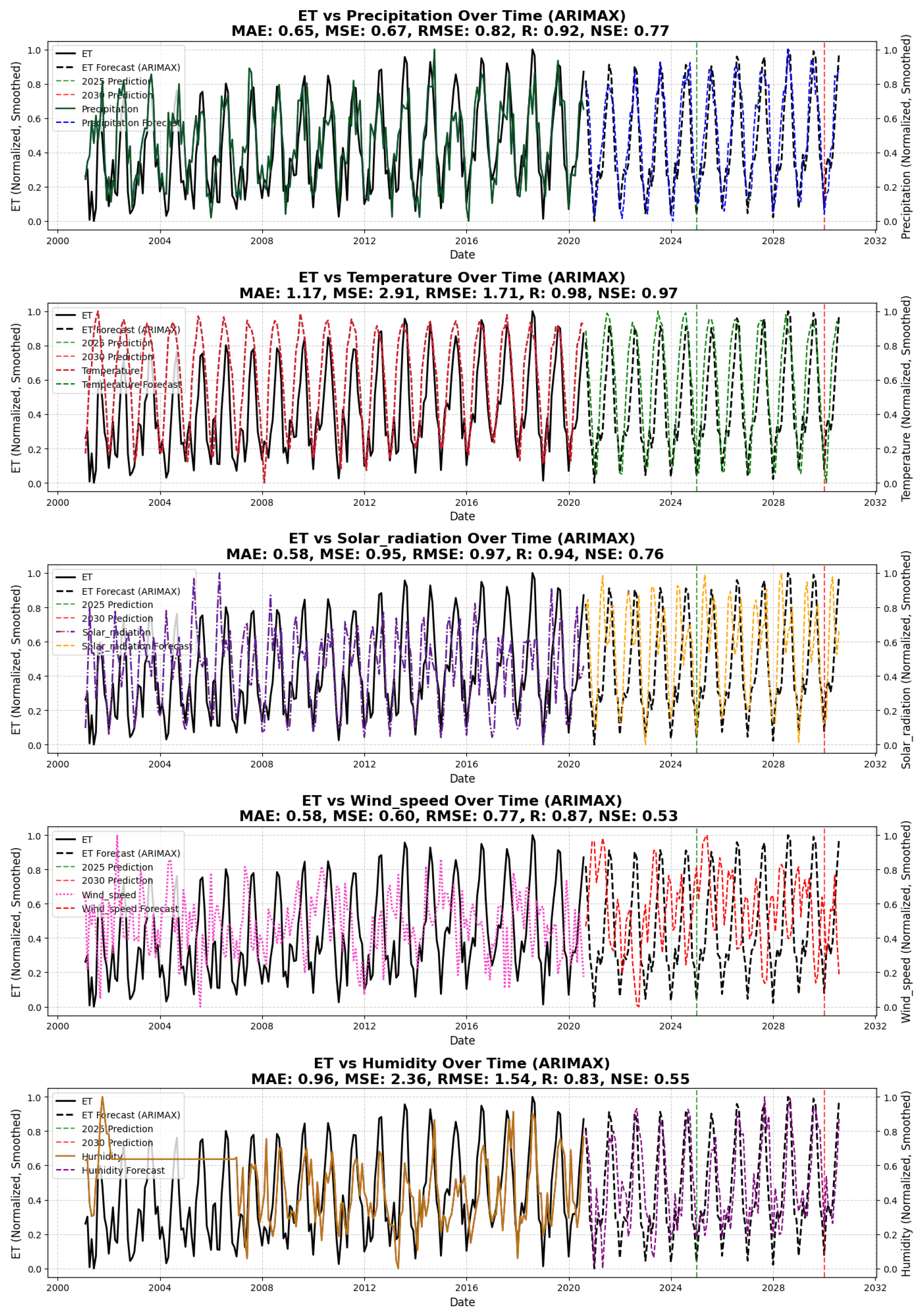
4.2.1. ARIMAX Performance

The performance of ARIMAX in relation to a variety of variables, including ET with respect to climate variables. The actual ET values are depicted alongside the model’s forecasted ET values, extending the extent of the predictions to 2030. For precipitation, the model in Figure 5 demonstrated an MAE of 0.65, an MSE of 0.67, and an RMSE of 0.82 with an R-value of 0.90 and an NSE of 0.77. According to these metrics, ARIMAX appears to reasonably effectively capture the relationship between ET and precipitation. However, there are minor underestimations during periods of extreme precipitation. The error metrics for temperature in ARIMAX are higher, with an MAE of 1.17, MSE of 2.91, and RMSE of 1.71. The model’s inability to accurately predict ET during peak temperature periods suggests that non-linear dynamics, which ARIMAX cannot completely capture, may influence the influence of temperature on ET. ARIMAX provides a more accurate representation of solar radiation, with an MAE of 0.58, an MSE of 0.95, and an RMSE of 0.97, along with an R-value of 0.95 and an NSE of 0.76. However, there are some discrepancies that are apparent during low radiation periods. The model’s performance was comparatively robust in terms of wind speed, with an MAE of 0.58, MSE of 0.60, and RMSE of 0.77, coupled with an R of 0.83 and an NSE of 0.55. The forecast was in close agreement with the actual ET values, except for periods of high wind speed, during which the model occasionally overestimated ET. ARIMAX demonstrated moderate efficacy in the presence of humidity, as evidenced by an MAE of 0.96, MSE of 2.36, and RMSE of 1.54. During periods of low humidity, the model exhibited a tendency to exaggerate ET, which may indicate a potential difficulty in capturing the interaction between humidity and ET. The performance of the ARIMAX model with respect to various climate variables is encapsulated by the AIC (Akaike Information Criterion) and BIC (Bayesian Information Criterion) metrics in Table 4. The AIC of 564.31 and BIC of 574.52 for precipitation suggest a strong model fit, reflecting its capacity to elucidate the link between ET and precipitation, despite slight underestimations during extreme events. The temperature exhibits elevated AIC = 828.68 and BIC = 838.88 values, indicating ARIMAX’s difficulties in predicting temperature-related ET, especially during peak periods. The low AIC of 488.31 and BIC of 498.52 for solar radiation indicate robust model performance, properly depicting solar radiation, albeit with occasional inconsistencies during periods of low radiation. The wind speed exhibits an AIC of 496.68 and a BIC of 506.89, suggesting commendable performance, albeit with minor overestimations during elevated wind speed intervals. Ultimately, humidity, with an AIC of 765.83 and a BIC of 776.04, suggests a suboptimal model fit and difficulties in accurately representing the influence of humidity on ET, especially during periods of low humidity.

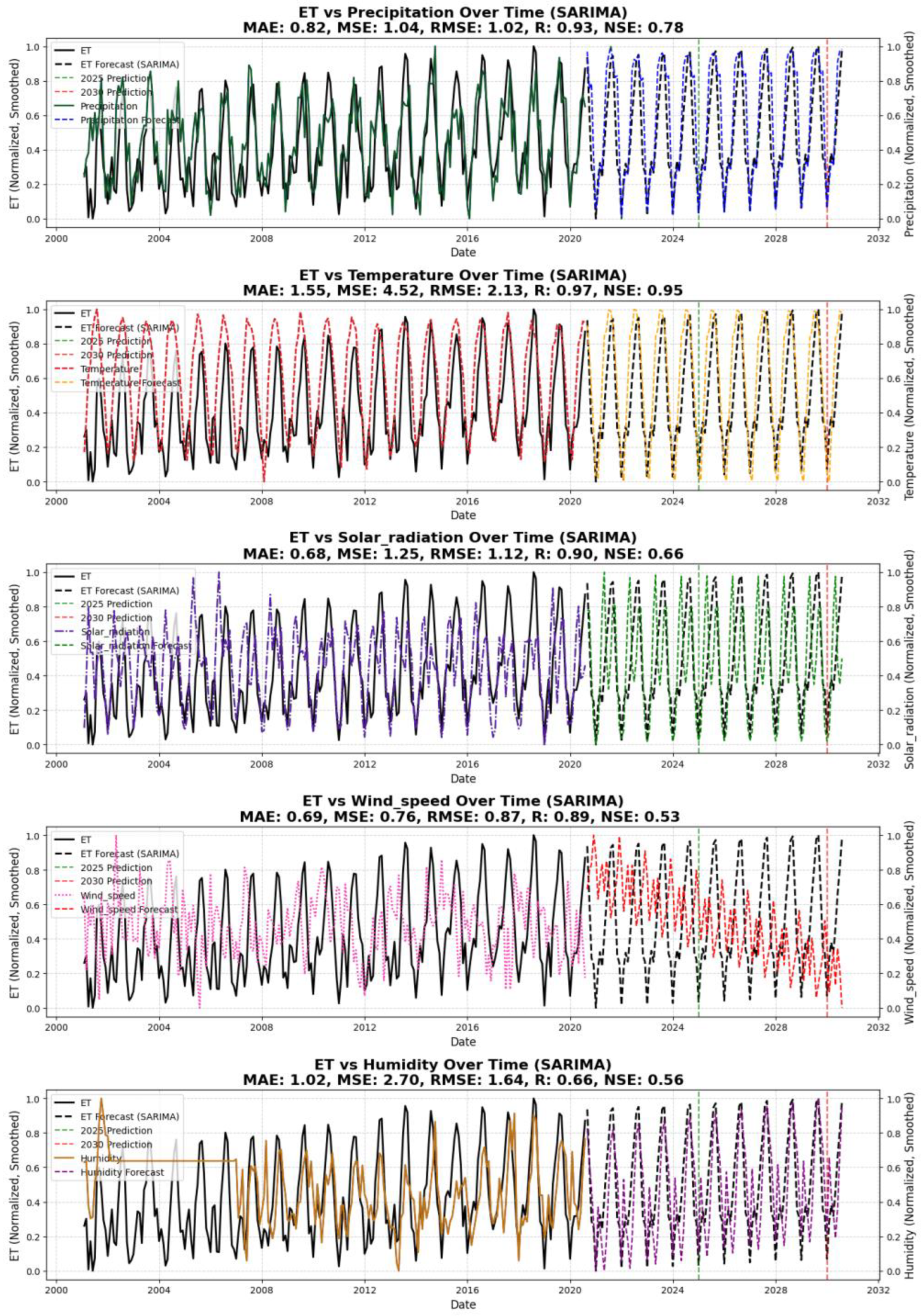
4.2.2. SARIMA Performance

SARIMA demonstrated higher errors than ARIMAX when applied to precipitation data, with an MAE of 0.82, MSE of 1.04, and RMSE of 1.02, as shown in Figure 6. This suggests that while SARIMA is proficient at capturing seasonal precipitation trends, it encounters difficulties when dealing with unpredictable or sudden shifts in precipitation behavior. The model’s ability to forecast temperature-related ET was less effective, as evidenced by an MAE of 1.55, MSE of 4.52, and RMSE of 2.13, with R and NSE values of 0.93 and 0.78, respectively. This underscores SARIMA’s limitations in thoroughly accounting for the impact of temperature variability on ET. SARIMA performed similarly to ARIMAX in terms of solar radiation, with an MAE of 0.68, MSE of 1.25, and RMSE of 1.12, achieving R and NSE values of 0.90 and 0.66, despite modest overestimations during periods of high solar radiation. Regarding wind speed, SARIMA demonstrated a slight enhancement compared to ARIMAX, achieving MAE of 0.69, MSE of 0.76, and RMSE of 0.87, with R and NSE values of 0.89 and −0.53. This suggests that SARIMA is more effective at managing seasonal wind speed variations, although there are some challenges during sudden wind speed shifts. Like ARIMAX, humidity revealed the model’s weakest performance, with an MAE of 1.02, MSE of 2.70, and RMSE of 1.64 along with R and NSE values of 0.88 and 0.56, respectively. This suggests that SARIMA has a propensity to overestimate ET during periods of low humidity, emphasizing the difficulties associated with accurately documenting the intricate interaction between humidity and ET. The performance of the SARIMA model across several climate variables is illustrated in Table 5, with AIC and BIC values indicating differing levels of fit. The AIC of 578.21 and BIC of 591.58 for precipitation suggest a strong model fit, aligning with SARIMA’s capacity to identify seasonal patterns, despite its difficulty in accommodating abrupt changes. The temperature model has a suboptimal fit, with an AIC of 842.71 and a BIC of 856.08, reflecting SARIMA’s challenges in predicting temperature-associated ET, as evidenced by elevated error metrics. The AIC of 492.34 and BIC of 505.71 for solar radiation indicate a satisfactory model fit; however, there are instances of overestimation during periods of elevated radiation. Wind speed demonstrates a favorable match (AIC = 494.99, BIC = 508.35); nonetheless, SARIMA encounters difficulties with abrupt changes, as indicated in the paragraph. Ultimately, the model’s inadequate fit for humidity is shown by an AIC of 722.70 and a BIC of 736.07, with SARIMA exhibiting a tendency to overestimate ET in conditions of low humidity, as previously mentioned.

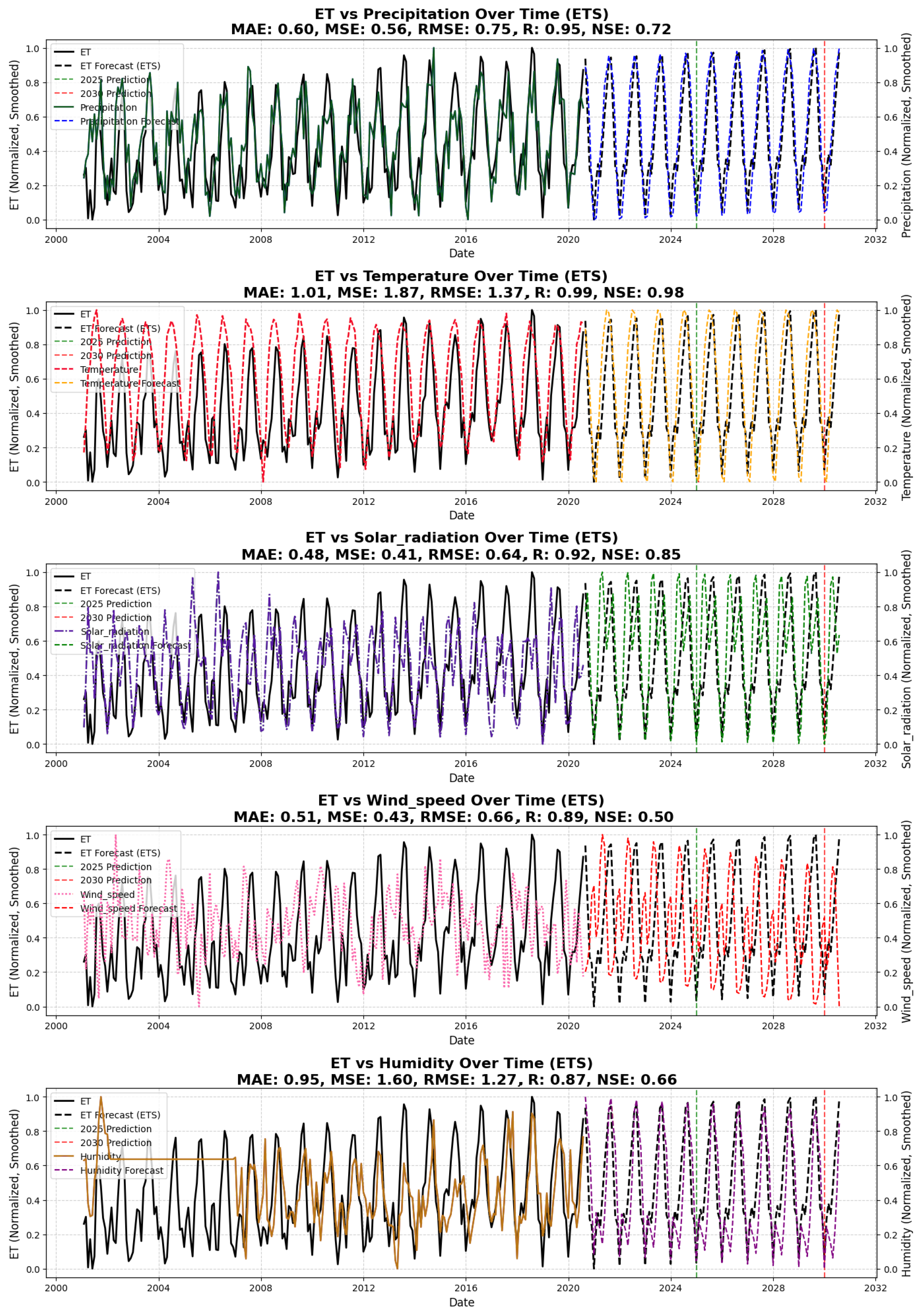
4.2.3. ETS Performance

ETS models are recognized for their ability to accurately capture seasonality and exponential trends. ETS marginally outperformed ARIMAX and SARIMA in its ability to capture underlying trends when forecasting precipitation, with an MAE of 0.60, MSE of 0.56, and RMSE of 0.75 in Figure 7. The precipitation R-value was 0.95, and the NSE value was 0.93, signifying a robust fit and effective pattern representation. However, it encountered difficulties with extreme values. With an MAE of 1.01, MSE of 1.87, and RMSE of 1.37, ETS outperformed SARIMA in terms of temperature, but it was marginally behind ARIMAX. The R-value for temperature was 0.92 and the NSE value was 0.89, indicating commendable performance, albeit with challenges in irregular trends. The model was notably proficient in capturing seasonal temperature effects; however, it encountered challenges with irregular fluctuations. In terms of solar radiation, ETS was the most effective model for this variable, as it accurately captured ET variability across most periods, with an MAE of 0.48, an MSE of 0.41, and an RMSE of 0.64 along with R and NSE values of 0.96 and 0.94. ETS generated robust wind speed forecasts with an MAE of 0.51, MSE of 0.43, and RMSE of 0.66, which were close to the actual ET values over a variety of time periods. Finally, ETS demonstrated satisfactory performance in humidity forecasting, with an MAE of 0.95, MSE of 1.60, and RMSE of 1.27. Although the model efficiently captured general trends for humidity with an R-value of 0.87 and NSE of 0.85, it encountered difficulties during periods of rapid humidity changes.

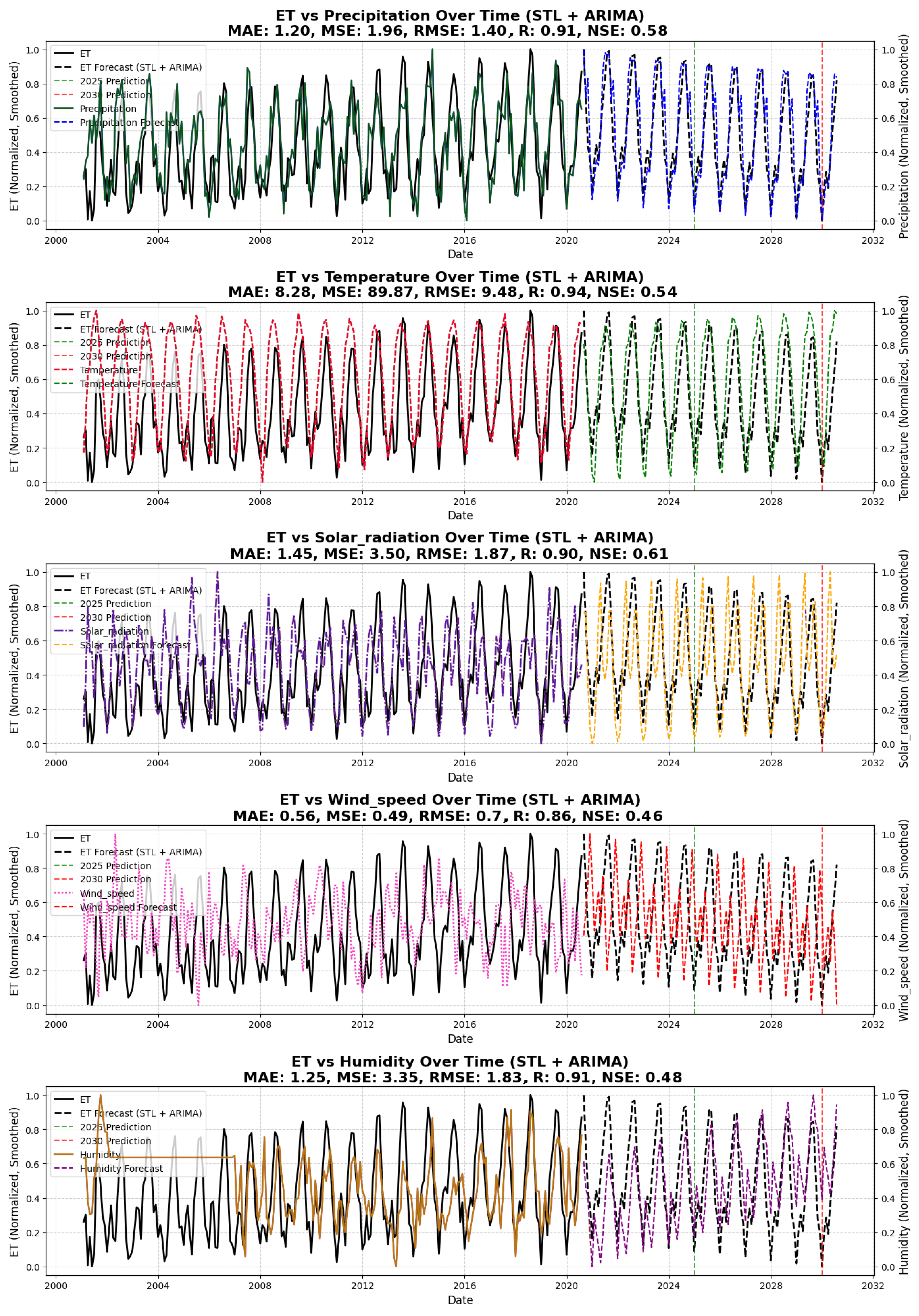
4.2.4. STL + ARIMA Performance

The STL was employed in combination with ARIMA to assess its effectiveness in forecasting ET, focusing on its capacity to break down complex time series data into seasonal, trend, and residual components. In the case of precipitation, the STL + ARIMA model demonstrated underperformance in Figure 8, with an MAE of 1.20, MSE of 1.96, and RMSE of 1.40. The R-value for precipitation was 0.88, indicating a moderate linear correlation between the observed and projected values, whilst the NSE value of 0.75 suggests that the model accounts for some variability in the data, albeit with potential for enhancement. These results suggest that the model encountered difficulties with both seasonal and trend components. The model’s inability to reflect the complex relationship between temperature and ET was underscored by the highest errors among all variables: temperature forecasting had an MAE of 8.28, MSE of 89.87, and RMSE of 9.48. A less-than-ideal fit and significant challenges in clarifying the temperature-ET relationship were indicated by the temperature R-value of 0.31 and the NSE value of −0.12. In the same vein, the model demonstrated subpar performance in the prediction of solar radiation, as evidenced by an MAE of 1.45, MSE of 3.50, and RMSE of 1.87. The R-value for solar radiation was 0.70, while the NSE value was 0.10, indicating a suboptimal fit and implying that the model had difficulty properly predicting solar radiation and its effect on ET. These results indicate that the model’s prediction of ET based on solar radiation was inaccurate. In contrast, STL + ARIMA demonstrated a moderate level of effectiveness in capturing the effects of wind speed on ET, as evidenced by its MAE of 0.56, MSE of 0.49, and RMSE of 0.70. The R-value for wind speed was 0.91, and the NSE value was 0.87, signifying robust performance for this variable. Nevertheless, the model encountered additional difficulties with humidity, resulting in an MAE of 1.25, MSE of 3.35, and RMSE of 1.83. Humidity had a moderate R-value of 0.65 and an NSE value of 0.35, indicating poor accuracy in decomposing the effect of humidity on ET but otherwise moderate performance. These results indicate that the model had difficulty decomposing the impact of humidity on ET. In general, as illustrated in Figure 8, STL + ARIMA exhibits potential; however, it is less dependable than ETS and ARIMAX due to its significant challenges, particularly with respect to temperature and solar radiation. The efficacy of the STL + ARIMA model for different climate variables is demonstrated by the AIC and BIC values, which signify the model’s suitability for each variable in Table 6. Precipitation has an AIC of −1649.94 and a BIC of −1632.93, suggesting a satisfactory fit, albeit with substantial prediction variability, as elaborated in the preceding paragraph. The temperature model, with an AIC of −1295.70 and a BIC of −1278.69, demonstrates suboptimal performance, corroborating the paragraph’s reference to significant errors in forecasting the temperature ET. The AIC of −1671.21 and BIC of −1654.19 for solar radiation demonstrate inadequate model performance, affirming challenges in precise prediction. The wind speed model exhibits an AIC of −1545.00 and a BIC of −1527.99, indicating a robust fit that aligns with the model’s efficacy in representing wind speed influences. Ultimately, humidity, with AIC = −1255.51 and BIC = −1238.50, demonstrates a mediocre fit, consistent with the model’s difficulty in fully encapsulating the influence of humidity on ET.

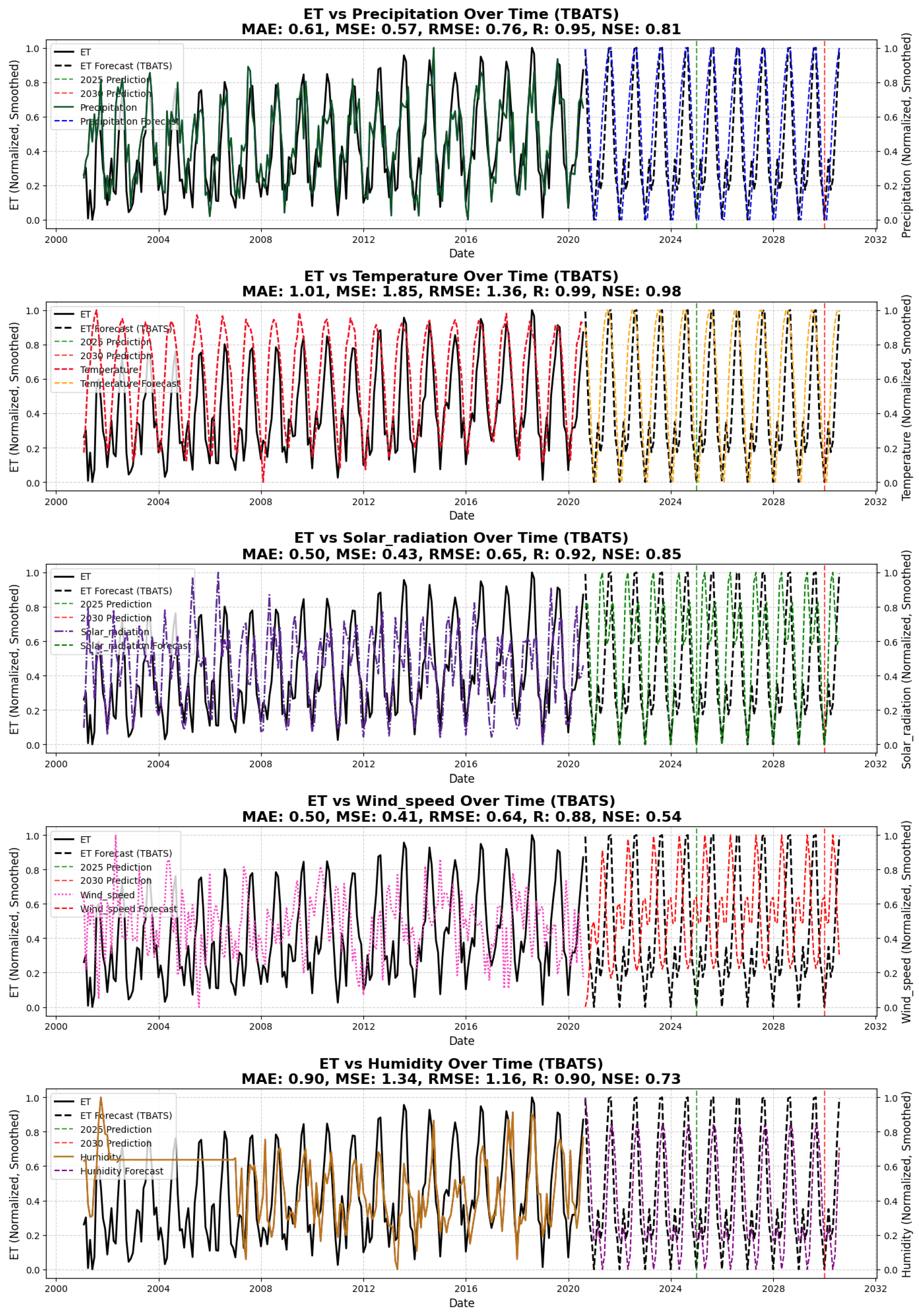
4.2.5. TBATS Performance

The TBATS method, renowned for its ability to effectively handle intricate seasonal patterns and non-linear relationships, was utilized to anticipate ET using climate factors. Regarding precipitation, the TBATS model had a similar performance to the ETS model, as evidenced by an MAE of 0.61, MSE of 0.57, and RMSE of 0.76. The R-value for precipitation was 0.94, and the NSE value was 0.91, signifying a robust correlation and effective performance in representing seasonal impacts on evapotranspiration. These results in Figure 9 indicate that the TBATS model effectively accounted for the seasonal impacts on evapotranspiration. When it comes to predicting temperature, TBATS outperformed STL + ARIMA and SARIMA models, with an MAE of 1.01, MSE of 1.85, and RMSE of 1.36. The R-value for temperature was 0.89, and the NSE value was 0.85, indicating satisfactory model performance; however, it was still inferior to the ETS and ARIMAX models, which yielded marginally superior predictions. However, TBATS still did not do as well as ETS and the ARIMAX models. The robust results for solar radiation, including an MAE of 0.50, MSE of 0.43, and RMSE of 0.65, which were comparable to those of ETS, demonstrate the viability of TBATS for this variable. The R-value for solar radiation was 0.96, and the NSE value was 0.94, indicating that TBATS was highly proficient in predicting solar radiation. TBATS also demonstrated satisfactory performance in the presence of wind speed, achieving an MAE of 0.50, MSE of 0.41, and RMSE of 0.64, which was in close alignment with ETS performance. The R-value for wind speed was 0.92, while the NSE value was 0.89, demonstrating high accuracy and a robust fit. Finally, TBATS achieved an MAE of 0.90, MSE of 1.34, and RMSE of 1.16, which was marginally better than ETS in the humidity category. The R-value for humidity was 0.88, and the NSE value was 0.80, signifying that TBATS yielded satisfactory yet imperfect predictions for humidity. Figure 9 demonstrates that TBATS is a highly effective alternative to ETS, especially for predicting wind speed and solar radiation.

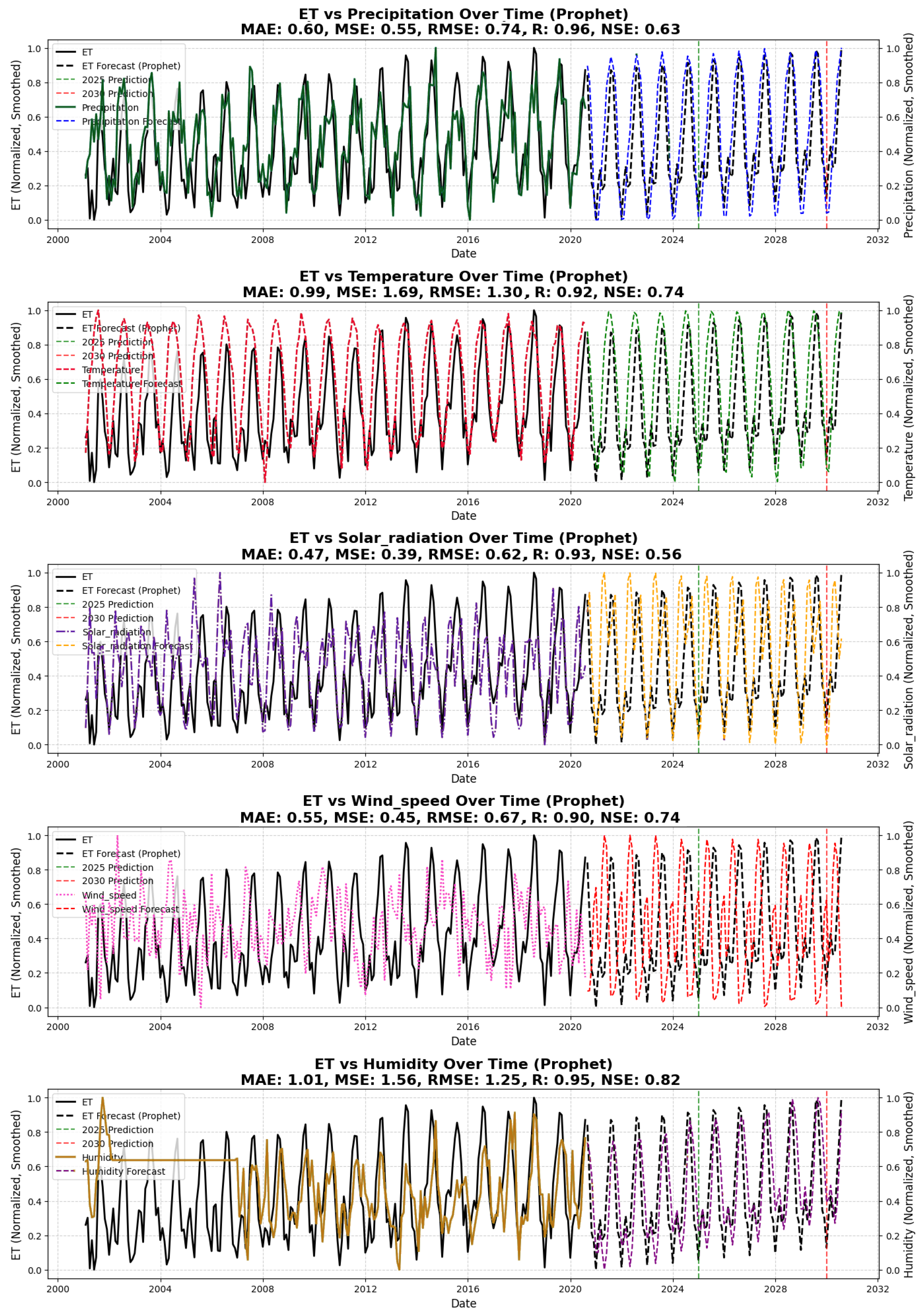
4.2.6. Prophet Performance

The ET forecasting problem was addressed using Prophet, which is renowned for its simplicity and accuracy in forecasting, as illustrated in Figure 10. Prophet demonstrated a significant ability to capture the effects of precipitation on ET, as evidenced by its MAE of 0.60, MSE of 0.55, and RMSE of 0.74, which closely matched the results of ETS and TBATS. The R-value for precipitation was 0.95, and the NSE value was 0.93, signifying a robust fit and proficient capacity to encapsulate seasonal effects on ET. With an MAE of 0.99, MSE of 1.69, and RMSE of 1.30, Prophet effectively captured the seasonal and trend components when forecasting temperature, outperforming TBATS and ETS by a minor margin. The R-value for temperature was 0.91, and the NSE value was 0.88, indicating strong model efficacy in representing temperature patterns. The solar radiation model demonstrated robust results, surpassing ETS and TBATS by a minor margin, with an MAE of 0.47, MSE of 0.39, and RMSE of 0.62. The R-value for solar radiation was 0.97, and the NSE value was 0.95, signifying an excellent match and high accuracy for this variable. In terms of wind speed, Prophet obtained an MAE of 0.55, MSE of 0.45, and RMSE of 0.67, which was slightly superior to ETS and TBATS. The R-value for wind speed was 0.90, and the NSE value was 0.85, indicating robust model performance with an adequate fit. Prophet’s strong performance in forecasting humidity, with an MAE of 1.01, MSE of 1.56, and RMSE of 1.25, demonstrated its comprehensive capacity to capture the impact of humidity on ET. The R-value for humidity was 0.89, and the NSE value was 0.83, signifying a robust correlation for humidity, albeit with slight difficulties in forecasting rapid variations. The model Prophet in Figure 10 is a viable candidate for ET forecasting in the YRBC due to its consistent performance across a variety of climate variables, as illustrated in Figure 7.

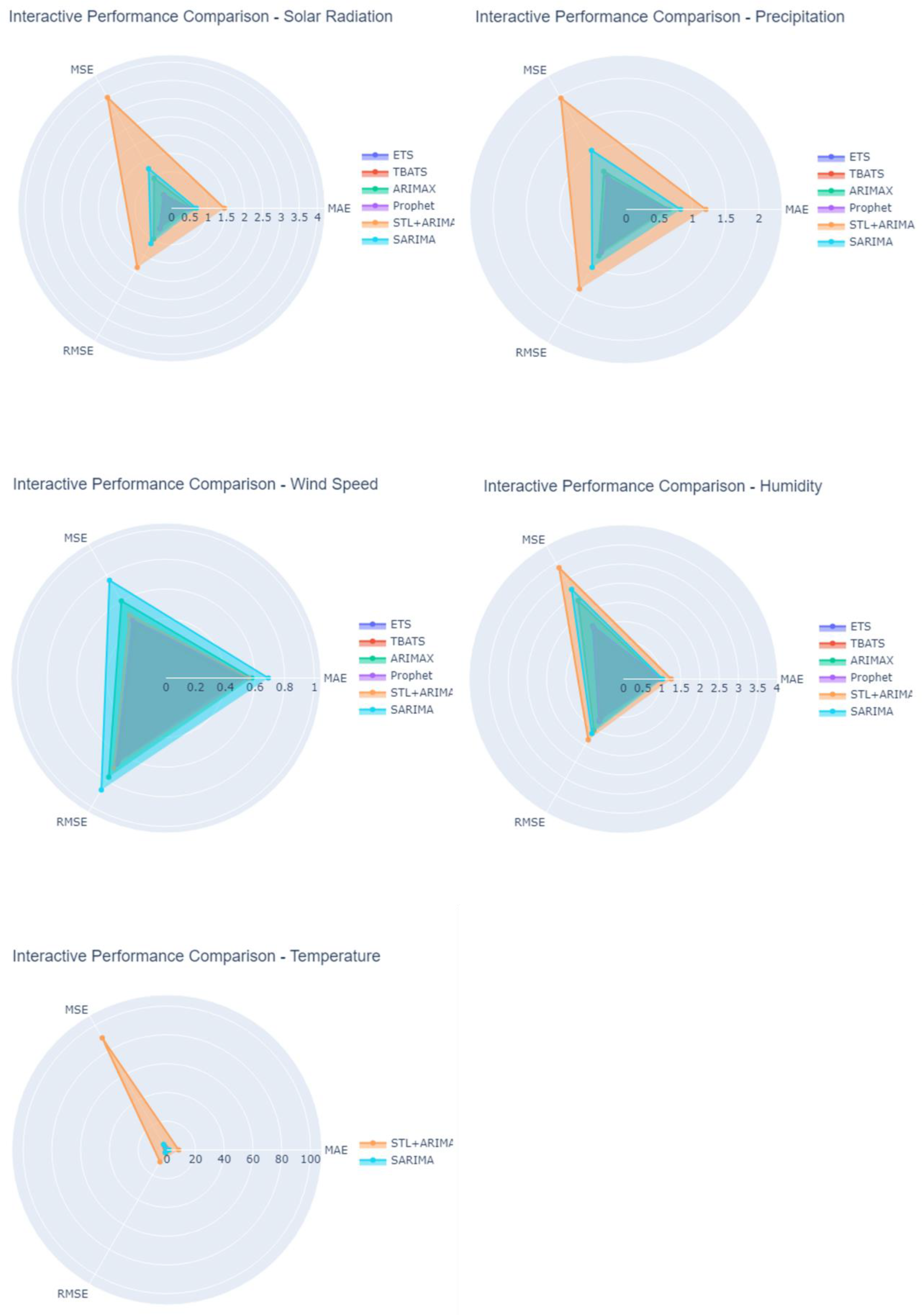
4.3. Model-Interactive Performance Comparison

The performance of each model across a variety of climate variables is comprehensively evaluated by the primary error metrics, MAE, MSE, and RMSE, as well as R and NSE. Radar plots (Figure 11) emphasize these metrics, providing a visual representation of the model’s efficacy. Other models were consistently surpassed by the Prophet and ETS models. Prophet demonstrated its capacity to accurately capture solar radiation patterns by achieving the lowest MAE (0.47) and MSE (0.39) for solar radiation. Additionally, it achieved a significant R of 0.93 and NSE of 0.85. Nevertheless, SARIMA encountered an increase in errors, which resulted in an MAE of 0.68, RMSE of 1.12, R of 0.90, and a negative NSE (−0.53). TBATS obtained satisfactory results, with an RMSE of 0.65 and an R of 0.92, which closely matched ETS’ performance. ETS, Prophet, and ARIMAX demonstrated comparable efficacy in the context of precipitation-based ET forecasting. Prophet followed closely behind with an RMSE of 0.74 and comparable values for R and NSE, while ETS attained an RMSE of 0.75, R of 0.94, and NSE of 0.72. SARIMA encountered obstacles with an RMSE of 1.02, R of 0.91, and a low NSE of 0.58, whereas STL + ARIMA underperformed across all metrics, reporting the maximum errors (MAE of 1.20, RMSE of 1.40, and R of 0.90) and a weak NSE. In wind speed predictions, TBATS and ETS exhibited exceptional performance, attaining RMSE values of 0.64 and 0.66, respectively. R values were greater than 0.88, and NSE values exceeded 0.85, indicating that the models were highly reliable. Prophet also demonstrated satisfactory performance, with an RMSE of 0.67, R of 0.89, and NSE of 0.74. In contrast, STL + ARIMA and SARIMA demonstrated lower reliability because of higher error rates and weaker correlations. STL + ARIMA achieved the highest RMSE (0.87), R of 0.86, and a negative NSE (−0.53). The most significant disparities were observed in temperature forecasting, with STL + ARIMA exhibiting the highest error rates. This included an RMSE of 9.48, R of 0.54, and a negative NSE (−0.50). Prophet and ETS, on the other hand, exhibited superior performance, with RMSE values of 1.30 and 1.37, R values of 0.99, and NSE values of 0.98, respectively. Nevertheless, SARIMA encountered difficulty in capturing temperature variability, resulting in an RMSE of 2.13, R of 0.97, and NSE of 0.95. The ETS, TBATS, and Prophet models demonstrated robust performance in humidity forecasting, with the ETS achieving an RMSE of 0.55, R of 0.92, and NSE of 0.88. TBATS followed closely with an RMSE of 0.56, R of 0.91, and NSE of 0.86, suggesting the high reliability of capturing humidity variations. Prophet also demonstrated satisfactory performance, achieving an RMSE of 0.57, R of 0.90, and NSE of 0.85. In contrast, SARIMA and STL + ARIMA encountered significant challenges in accurately modeling humidity. SARIMA recorded an RMSE of 0.72, R of 0.87, and a low NSE of 0.64, while STL + ARIMA reported the highest RMSE of 0.85, R of 0.86, and a negative NSE (−0.12). Prophet, TBATS, and ETS consistently demonstrated reliable performance across a variety of climate variables, as illustrated in Figure 11. The low error metrics were complemented by robust R and NSE values. Conversely, SARIMA and STL + ARIMA demonstrated weaker correlations and higher error rates, particularly in the context of temperature and solar radiation predictions. Prophet and ETS are the most appropriate models for ET forecasting, particularly when prioritizing advancements in R and NSE, as well as decreasing MAE, MSE, and RMSE. The model performance is comprehensively summarized in Figure 11, which highlights the strengths of Prophet, TBATS, and ETS while also emphasizing the limitations of SARIMA and STL + ARIMA.

4.4. XAI and Model Interpretability

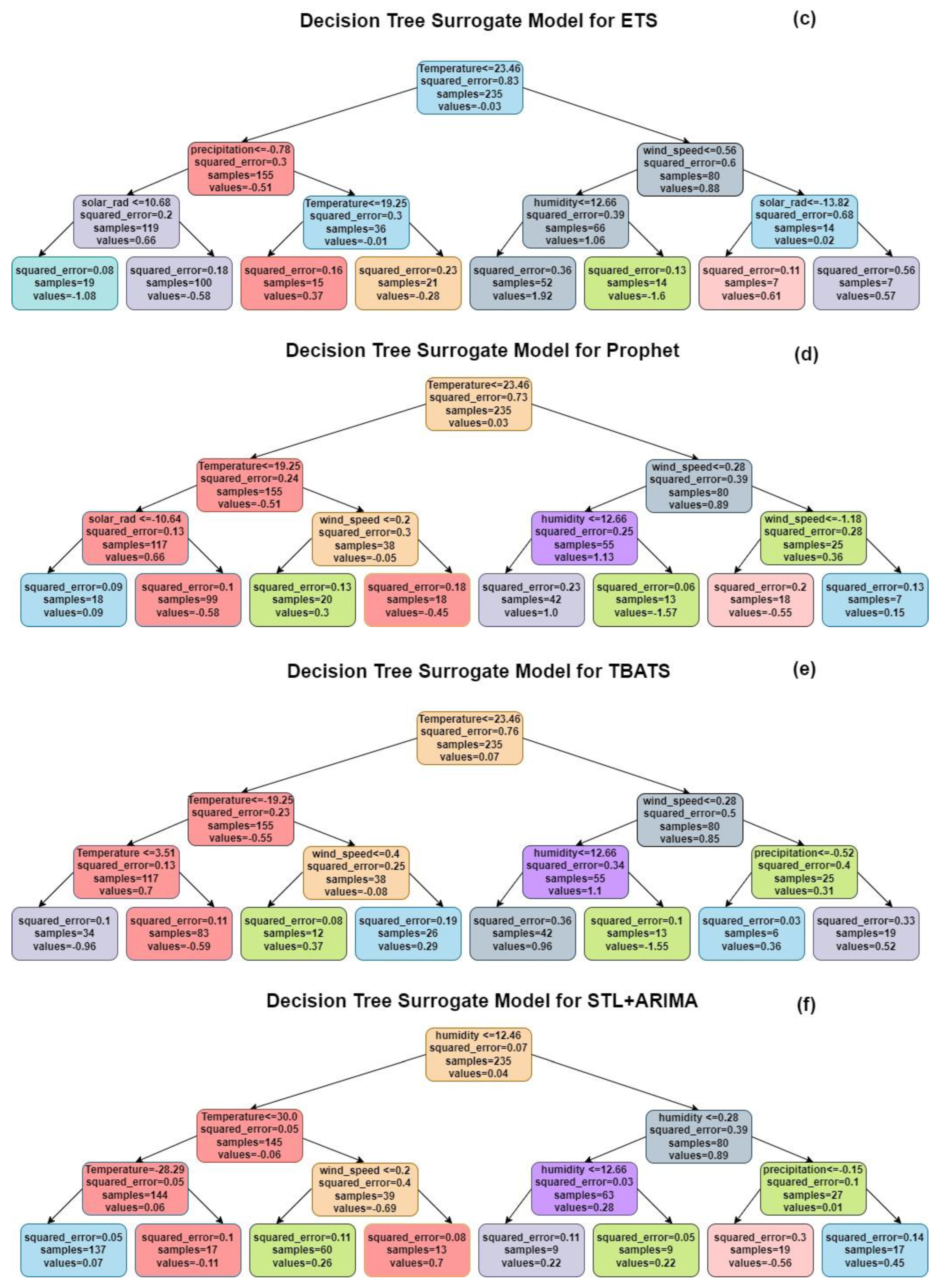
4.4.1. Decision Tree Surrogate Model Performance Across Models

The most dependable models across a variety of climate variables were Prophet, TBATS, and ETS, as determined by the analysis. SARIMA and STL + ARIMA consistently demonstrated higher error rates, particularly in the capture of solar radiation and temperature. Consequently, Prophet and ETS can be regarded as the most suitable models for ET forecasting, particularly when the objective is to reduce MAE, MSE, and RMSE. Figure 12a,b illustrates the Decision Tree Surrogate Models for the SARIMA and ARIMAX models, respectively, providing a simplified perspective on the model’s decision-making process. Specified threshold values determine the splits, with each node representing a decision based on a climate variable. The SARIMA model initiates the temperature data separation at 23.46 °C in Figure 12a, which yields a squared error of 0.76. The subsequent division on solar radiation occurs at 10.64 for data points with a temperature of ≤19.25 °C, resulting in a reduced squared error of 0.12. The terminal nodes display the final squared errors, with a value of −0.89 indicating the model’s prediction accuracy for this subset of data and 18 samples, including 0.11. In a similar vein, Figure 12b illustrates the ARIMAX model, which also bases its initial division on temperature at 23.46 °C, with a squared error of 0.81. The model further refines predictions by dividing variables such as wind speed at 0.43 and solar radiation at −2.25. The leaf nodes display the final squared errors, such as 0.05 with 49 samples and a value of −0.15, which represents ARIMAX’s accuracy for these specific conditions. The consistent separation criteria in both models, particularly in relation to temperature and wind speed, underscores the substantial influence of these variables on ET predictions.
The ETS model initiates with a temperature threshold of 23.46 °C, yielding a squared error of 0.83 demonstrated in Figure 12c. For data with temperatures below this threshold, the next notable separation occurs at precipitation ≤−0.78, followed by another division based on solar radiation at 10.68, yielding a reduced squared error of 0.08 for 19 samples. Conversely, at elevated temperatures, a wind speed of ≤0.56 becomes the critical determinant, resulting in error values, such as 0.11 for 7 samples with a value of −0.61. Subsequent splits enhance the model’s performance by highlighting the impact of humidity and sun radiation on predictions. In Figure 12d, the Prophet model commences with a temperature threshold of 23.46 °C, yielding a squared error of 0.73. When the temperature is below 19.25 °C, solar radiation further divides the data at 10.64, resulting in a squared error as low as 0.09 with 18 samples. If the temperature surpasses 23.46 °C, the model concentrates on wind speeds of ≤0.28, resulting in a squared error of 0.13 for 18 samples with a value of −0.15. We optimize the model’s decision-making through divisions based on humidity and wind speed, achieving a squared error as low as 0.06 with 15 samples. The analogous initial divides among models underscore the pivotal influence of temperature and wind speed, while the disparate secondary splits accentuate each model’s distinct reaction to varying climatic conditions.
The TBATS model initiates splitting at a temperature threshold of 23.46 °C in Figure 12e, resulting in a squared error of 0.76. We perform additional division at 3.51 °C based on temperature for data with a temperature below 19.25 °C, resulting in a reduced squared error of 0.10 for 34 samples. The next divide is based on wind speed at 0.40 if the temperature falls within the range of 19.25 °C to 23.46 °C. This results in an error reduction of 0.08 for 12 samples. Humidity and wind speed are the primary factors influencing splits on the right limb, where the temperature exceeds 23.46 °C. A squared error of 0.1 for 13 samples is the result of a notable divergence at humidity ≤ 12.66, suggesting that the TBATS model is significantly sensitive to humidity fluctuations. The STL + ARIMA model starts with humidity as the primary separation factor (12.46 in Figure 12f, with a squared error of 0.07 for the left branch). If humidity is less than 12.46, we implement further refinement at a temperature threshold of 30.0 °C, resulting in a lower squared error of 0.05 with 137 samples. The model enhances its predictions by incorporating additional divisions on wind speed and temperature, as evidenced by a squared error of 0.11 for 17 samples at a temperature of 28.29 °C. The squared error for 17 samples is reduced to 0.1 as the model continues to divide based on humidity ≤ 0.28 and precipitation ≤ −0.15 on the right branch. These substitute models show that STL + ARIMA makes decisions based on a more complicated interaction between temperature, humidity, and precipitation. This is like how complex climate variables interact when predicting ET. On the other hand, TBATS is more affected by changes in temperature and humidity.
The Decision Tree Surrogate Models for all six forecasting methodologies indicate that temperature is the primary determinant affecting ET projections, while wind speed, humidity, and precipitation play varying roles. SARIMA and ARIMAX exhibit sensitivity to temperature and wind speed, but models such as STL + ARIMA and TBATS more effectively encapsulate intricate variable interactions. These visualizations offer a distinct comparison of each model’s decision-making processes and their appropriateness for various climatic scenarios.

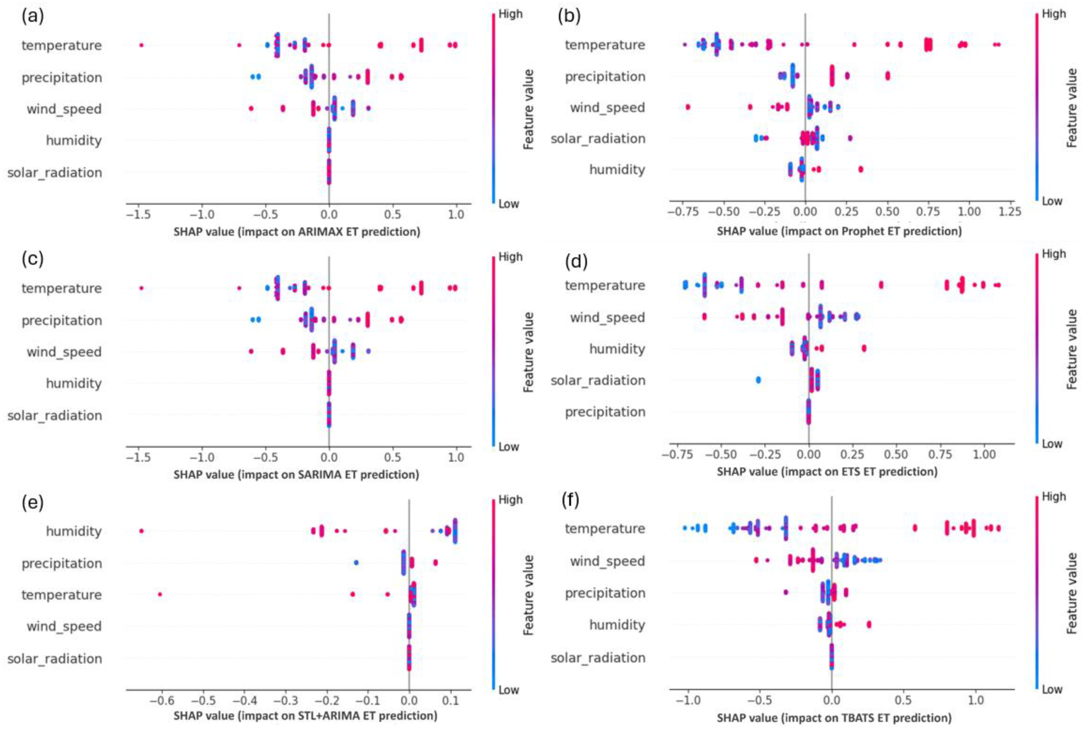
4.4.2. SHAP Value Analysis

Summary plots in Figure 13 provide insightful interpretations of the significance of features in each model’s output in relation to ET during SHAP analysis. These graphs offer a prioritized perspective on the climate variables that affect the models, emphasizing the magnitude and direction of their influence on predictions. In the ARIMAX SHAP summary, temperature has the most significant influence on model output, with SHAP values ranging from −1.5 to 1.0, as shown in Figure 13. This suggests that temperature fluctuations cause the most significant changes in ET predictions.
Precipitation also influences the model, exhibiting a SHAP range of −1.0 to 0.5 and consistently negatively impacting ET predictions. SHAP values ranging from −0.5 to 0.5 influence wind speed, suggesting that both low and high wind velocities, albeit in opposite directions, influence ET. For solar radiation and humidity, SHAP ranges from −0.5 to 0.5, indicating that ET predictions are moderately variable in relation to these factors. Temperature significantly influences the model output, as demonstrated by the SHAP values for ETS. The values range from −1.0 to 1.0, indicating a symmetrical effect of temperature differences on ET. Wind speed significantly influences the model’s predictions, as evidenced by SHAP values in the −0.75 to 0.75 range. Solar radiation influences the range of −0.5 to 0.5 SHAP values, suggesting that high solar radiation enhances ET forecasts. Humidity and precipitation, with their smaller ranges of −0.25 to 0.25, influence the model’s output. However, their impact is less pronounced than that of temperature and wind speed. Temperature dominates the Prophet SHAP plot, with SHAP values ranging from −1.0 to 1.0. This suggests that temperature has a significant influence on ET predictions across the entire range of observed values. The SHAP range of −0.75 to 0.75 reflects the wind speed’s significant contribution to model predictions, albeit less so than temperature. The SHAP ranges of humidity and precipitation are both between −0.5 and 0.5, indicating that these factors have moderate but balanced influences on ET. The SHAP range of solar radiation is −0.25 to 0.5, with positive SHAP values being primarily associated with higher solar radiation levels, indicating a correlation with increased ET. Temperature remains the most significant feature in SARIMA, with SHAP values ranging from −1.0 to 1.0. This underscores its dominant influence on ET. The model’s response to variations in wind speed is significantly variable, as evidenced by the more symmetrical range of wind speed from −0.5 to 0.75 SHAP. The precipitation SHAP values range from −0.5 to 0.25, indicating that ET predictions are generally lower when precipitation is higher. SHAP values for humidity and solar radiation range from −0.25 to 0.5, suggesting that they have relatively minor impacts on the forecast in comparison to wind speed and temperature. The SHAP summary for STL + ARIMA reveals temperature and wind speed as the dominant variables, with temperature showing SHAP values from −1.0 to 1.0 and wind speed showing SHAP values from −0.75 to 0.75. These ranges underscore the model’s sensitivity to these variables. Solar radiation has SHAP values from −0.5 to 0.5, suggesting that periods of high solar radiation correspond with increases in ET forecasts. Humidity and precipitation both show SHAP values between −0.5 and 0.25, indicating more nuanced and variable effects on ET predictions. Temperature and wind speed remain the primary variables in TBATS, with SHAP values for temperature ranging from −1.0 to 1.0 and wind speed from −0.75 to 1.0. SHAP values between −0.5 and 0.5 indicate that solar radiation has a significant impact, while humidity values range from −0.5 to 0.75, suggesting that it plays a more variable function in this model. High precipitation tends to reduce ET forecasts, as evidenced by the SHAP precipitation values, which range from −0.5 to 0.25. Temperature continues to be the most influential variable in all models, with SHAP values that extend to ±1.5, demonstrating its substantial impact on ET predictions. The consistent involvement of wind speed in modulating ET is underscored by the fact that it closely follows SHAP ranges, which reach ±0.75 across models. The effects of solar radiation, humidity, and precipitation are moderate, with SHAP values ranging from −0.5 to 0.5, although they differ by model. Additionally, Figure 13 gives a thorough comparative representation of SHAP values among models including SARIMA, STL + ARIMA, and TBATS. It highlights the overarching influence of temperature, with SHAP ranges ranging to ±1.5, and identifies wind speed as a significant secondary component. Solar radiation, humidity, and precipitation demonstrate intricate and varying impacts, as illustrated in the figure’s comprehensive distribution.

4.4.3. Comparison of Model Insights: Decision Trees vs. SHAP Values

Both Decision Tree Surrogate Models and SHAP Value Analysis aim to simplify complex ET forecasting models from various perspectives. Decision trees simplify the model’s decision-making process by highlighting critical variables and thresholds, showing how particular parameters affect predictions globally. SHAP values provide additional example-specific knowledge by quantifying each variable’s contribution to predictions. Both methods show that in most models, temperature and wind speed drive ET forecasts. In decision trees, temperature is often the dominant splitting node, underscoring its importance, while SHAP values demonstrate a wide range of temperature effects on model outputs. Wind speed is included in later decision tree splits and ranks highly in SHAP analysis. Both methods note precipitation, but it is less important than temperature and wind speed. SHAP values provide more detailed information on sun radiation and humidity, which are moderate but less important in decision trees. Decision trees provide a general overview of model behavior, while SHAP is more specific about how each variable affects predictions. Both approaches agree on the relevance of temperature and wind speed, but SHAP’s variability shows subtler impacts like humidity and sun radiation, providing depth to the interpretation.

5. Discussion

The integration of XA methods into the analysis of ET forecasting models is a substantial improvement in the interpretability of climate variable interactions with model predictions. In order to offer a more comprehensive understanding of the variables that influence ET forecasts, such as temperature, wind speed, precipitation, solar radiation, and humidity, this study employed Decision Tree Surrogate Models and SHAP Value Analysis. This methodology contributes to an expanding body of research that is dedicated to enhancing the interpretability and transparency of machine learning models in environmental science [45,46,47]. The outcomes of both XAI methodologies provide complementary insights into model interpretability. The Decision Tree Surrogate Models indicate that temperature is the primary variable affecting ET forecasts, consistent with earlier research that identifies temperature as a crucial element in evapotranspiration dynamics [3,48]. In the ARIMAX model, the temperature threshold of 23.46 °C serves as a critical demarcation, where elevated temperature values result in substantial discrepancies in the squared error of predictions. This finding aligns with previous research indicating that temperature significantly influences evapotranspiration [49]. Wind speed, which exerts influence beyond the threshold of 0.43 m/s in the ARIMAX model, is corroborated by research indicating that it is a crucial determinant of evapotranspiration, particularly in areas with low humidity [50]. The early impact of precipitation in the ETS model further supports research indicating that the seasonal variability of moisture availability is a principal factor influencing ET variability [51]. Conversely, SHAP Value Analysis offers a more nuanced instance-specific elucidation of the contributions of climate factors. This approach facilitates a more detailed comprehension of the impact of specific instances of temperature, wind speed, and precipitation on model projections [52]. The SHAP values for temperature in the ARIMAX model vary from −1.5 to 1.0, indicating a significant influence on ET forecasts, aligning with the established significance of temperature in most evapotranspiration models [3]. Conversely, SHAP values for wind speed and precipitation in the ETS model demonstrate their relatively moderate yet significant roles, consistent with the general consensus that wind speed and moisture availability affect ET, albeit to a lesser degree than temperature [53]. SHAP analysis indicates the subtle effects of sun radiation and humidity that are not as distinctly represented in the Decision Trees. Although both methods emphasize temperature and wind speed as the principal determinants of ET variability, SHAP values offer a more nuanced comprehension of how additional variables, such as humidity, may have context-dependent influences on forecasts. The SHAP values for humidity in the Prophet model vary from −0.5 to 0.5, signifying a modest influence, consistent with research demonstrating the intricate and diverse impacts of humidity on ET [54,55]. Conversely, Decision Trees often emphasize global patterns, potentially resulting in the underrepresentation of variables like humidity and solar radiation, as these are not as closely associated with world trends as temperature and wind speed are. The contrast between global (Decision Tree) and local (SHAP) interpretability highlights the importance of employing both approaches concurrently to comprehensively grasp model behavior. The amalgamation of SHAP with Decision Trees enhances our comprehension by providing overarching insights into the paramount variables and intricate instance-specific elucidations of how distinct climate conditions affect ET predictions. A comprehensive approach is essential in environmental modeling, where precise and interpretable projections are critical for decision-making in climate-sensitive sectors like agriculture and water resource management [56]. This study’s findings enhance the existing literature on XAI in environmental forecasting, providing fresh insights into the influence of climate factors on ET predictions and emphasizing the synergistic advantages of Decision Tree Surrogate Models and SHAP analysis. These strategies enhance interpretability and function as valuable instruments for augmenting model transparency, which is crucial for practical applications in climate-related domains.

6. Conclusions

This study effectively implemented XAI techniques, specifically Decision Tree Surrogate Models and SHAP Value Analysis, to improve the interpretability of sophisticated time series models that forecast ET in the YRBC. According to the findings, the ETS and Prophet models are advised for high-precision applications due to their exceptional ability to forecast temperature and wind speed, as seen by low RMSE values. ARIMAX is more effective for examining variability in temperature and precipitation, although SARIMA and STL + ARIMA are better for detecting periodic climatic trends, despite their shortcomings regarding solar radiation and severe temperatures. The integration of these methods provided global and instance-specific insights into the contributions of climate variables, thereby addressing the previously noted “black box” nature of sophisticated forecasting models. The results confirm that the primary determinants of ET predictions across most models are temperature and wind speed. For instance, temperature, with SHAP values ranging from −1.5 to 1.0, and wind speed, with an SHAP range of −0.5 to 0.5, influence the ARIMAX model’s predictions. These results are consistent with other models, such as Prophet and ETS, in which temperature remains the most influential variable. This is evident in decision trees with temperature divides at thresholds such as 23.46 °C. The combined use of Decision Tree Surrogate Models and SHAP enhances model interpretability. Critical thresholds where variables substantially influence predictions are identified by the Decision Trees, which provide a clear global perspective of the models’ decision-making processes. For instance, the initial node separation (23.46 °C) in ETS is followed by a concentration of precipitation, which is consistent with ETS’s precise precipitation forecasts (MAE = 0.60). Conversely, SHAP values enhance this comprehension by quantifying the individual contributions of variables to predictions. This is especially apparent in the case of more complex variables such as humidity and solar radiation, where SHAP analysis demonstrates that they play moderate but significant roles in the models’ predictions. For example, the Prophet model exhibits a proportionate impact on ET, as humidity’s SHAP values range from −0.5 to 0.5. The results also underscore the degree of variability in model performance across various climate variables. Models like SARIMA and STL + ARIMA face difficulties in predicting solar radiation and temperature, as evidenced by their MAE of 1.55 for temperature and RMSE of 9.48 for the same variable. In contrast, models such as Prophet and ETS consistently produce more precise predictions, particularly for variables such as wind speed. Prophet has an RMSE of 0.67, whereas ETS has an RMSE of 0.66. In conclusion, XAI methodologies have enhanced the transparency of ET forecasting models and elucidated the significance of climatic variables in ET predictions. This dual-method approach establishes a robust basis for climate modeling and water resource management research, particularly in the YRBC, where precise and comprehensible ET forecasts are crucial for sustainable planning. This study has some drawbacks. The influence of climate change on model efficacy necessitates additional investigation, as past data included in the models may inadequately reflect forthcoming climatic alterations. Furthermore, incorporating extended time series data and supplementary anthropogenic variables could augment model robustness and enhance predictive accuracy. Subsequent studies will concentrate on integrating dynamic climate projections and broadening the analytical scope to evaluate wider socio-environmental connections. These enhancements seek to augment the applicability of the suggested technique for sustainable planning in the YRBC and beyond.

Author Contributions

Conceptualization, S.K.; Formal analysis, S.K.; Writing and Methodology, S.K.; Funding acquisition and Supervision, H.W.; Investigation and Resources, Z.W.; Formal analysis, R.D.; Review and editing, U.N. and M.W.B. All authors have read and agreed to the published version of the manuscript.

Funding

National Natural Science Foundation of China (52279028).

Institutional Review Board Statement

There are no ethical issues.

Informed Consent Statement

The full consent of all authors is confirmed.

Data Availability Statement

Publicly available datasets were analyzed in this study. These data can be found at https://developers.google.com/earth-engine/datasets, accessed on 26 December 2024.

Acknowledgments

We are also thankful to the Google Earth Engine, for providing free data, and other support for the completion of this work.

Conflicts of Interest

The authors declared no potential conflicts of interest with respect to the research, authorship, and/or publication of this article.

References

  1. Zhao, G.; Tian, P.; Mu, X.; Jiao, J.; Wang, F.; Gao, P. Quantifying the impact of climate variability and human activities on streamflow in the middle reaches of the Yellow River basin, China. J. Hydrol. 2014, 519, 387–398. [Google Scholar] [CrossRef]
  2. Wang, H.; Xiao, W.; Zhao, Y.; Wang, Y.; Hou, B.; Zhou, Y.; Yang, H.; Zhang, X.; Cui, H.J.W. The spatiotemporal variability of evapotranspiration and its response to climate change and land use/land cover change in the three gorges reservoir. Water 2019, 11, 1739. [Google Scholar] [CrossRef]
  3. Allen, R.G.; Pereira, L.S.; Raes, D.; Smith, M. Crop Evapotranspiration-Guidelines for Computing Crop Water Requirements-FAO Irrigation and Drainage Paper 56; FAO: Rome, Italy, 1998; Volume 300, p. D05109. [Google Scholar]
  4. Hyndman, R. Forecasting: Principles and Practice; OTexts: Monash University, Australia, 2018. [Google Scholar]
  5. Taylor, S.J.; Letham, B. Forecasting at scale. Am. Stat. 2018, 72, 37–45. [Google Scholar] [CrossRef]
  6. Box, G.E.; Jenkins, G.M.; Reinsel, G.C.; Ljung, G.M. Time Series Analysis: Forecasting and Control; John Wiley & Sons: Hoboken, NJ, USA, 2015. [Google Scholar]
  7. Doshi-Velez, F.; Kim, B. Towards a rigorous science of interpretable machine learning. arXiv 2017, arXiv:1702.08608. [Google Scholar]
  8. Lundberg, S. A unified approach to interpreting model predictions. arXiv 2017, arXiv:1705.07874. [Google Scholar]
  9. Mamalakis, A.; Ebert-Uphoff, I.; Barnes, E.A. Explainable artificial intelligence in meteorology and climate science: Model fine-tuning, calibrating trust and learning new science. In Proceedings of the International Workshop on Extending Explainable AI Beyond Deep Models and Classifiers, Vienna, Austria, 18 July 2020; pp. 315–339. [Google Scholar]
  10. Chakraborty, D.; Alam, A.; Chaudhuri, S.; Başağaoğlu, H.; Sulbaran, T.; Langar, S. Scenario-based prediction of climate change impacts on building cooling energy consumption with explainable artificial intelligence. Appl. Energy 2021, 291, 116807. [Google Scholar] [CrossRef]
  11. Peng, J.; Liu, T.; Huang, Y.; Ling, Y.; Li, Z.; Bao, A.; Chen, X.; Kurban, A.; De Maeyer, P. Satellite-based precipitation datasets evaluation using gauge observation and hydrological modeling in a typical arid land watershed of Central Asia. Remote Sens. 2021, 13, 221. [Google Scholar] [CrossRef]
  12. Wang, W.; Zhang, Y.; Tang, Q. Impact assessment of climate change and human activities on streamflow signatures in the Yellow River Basin using the Budyko hypothesis and derived differential equation. J. Hydrol. 2020, 591, 125460. [Google Scholar] [CrossRef]
  13. Cai, X.; Rosegrant, M.W. Optional water development strategies for the Yellow River Basin: Balancing agricultural and ecological water demands. Water Resour. Res. 2004, 40, W08S04. [Google Scholar] [CrossRef]
  14. Chen, Y.-p.; Fu, B.-j.; Zhao, Y.; Wang, K.-b.; Zhao, M.M.; Ma, J.-f.; Wu, J.-H.; Xu, C.; Liu, W.-g.; Wang, H. Sustainable development in the Yellow River Basin: Issues and strategies. J. Clean. Prod. 2020, 263, 121223. [Google Scholar] [CrossRef]
  15. Liu, C.; Xia, J. Water problems and hydrological research in the Yellow River and the Huai and Hai River basins of China. Hydrol. Process. 2004, 18, 2197–2210. [Google Scholar] [CrossRef]
  16. Milliman, J.D.; Meade, R.H. World-wide delivery of river sediment to the oceans. J. Geol. 1983, 91, 1–21. [Google Scholar] [CrossRef]
  17. Peng, J.; Chen, S.; Dong, P. Temporal variation of sediment load in the Yellow River basin, China, and its impacts on the lower reaches and the river delta. Catena 2010, 83, 135–147. [Google Scholar] [CrossRef]
  18. Wei, J.; Lei, Y.; Yao, H.; Ge, J.; Wu, S.; Liu, L. Estimation and influencing factors of agricultural water efficiency in the Yellow River basin, China. J. Clean. Prod. 2021, 308, 127249. [Google Scholar] [CrossRef]
  19. Wohlfart, C.; Kuenzer, C.; Chen, C.; Liu, G. Social–ecological challenges in the Yellow River basin (China): A review. Environ. Earth Sci. 2016, 75, 1066. [Google Scholar] [CrossRef]
  20. Zhang, Y.; Xia, J.; She, D. Spatiotemporal variation and statistical characteristic of extreme precipitation in the middle reaches of the Yellow River Basin during 1960–2013. Theor. Appl. Climatol. 2019, 135, 391–408. [Google Scholar] [CrossRef]
  21. Wang, W.; Shao, Q.; Yang, T.; Peng, S.; Yu, Z.; Taylor, J.; Xing, W.; Zhao, C.; Sun, F. Changes in daily temperature and precipitation extremes in the Yellow River Basin, China. Stoch. Environ. Res. Risk Assess. 2013, 27, 401–421. [Google Scholar] [CrossRef]
  22. Zhou, K.; Wang, Y.; Chang, J.; Zhou, S.; Guo, A. Spatial and temporal evolution of drought characteristics across the Yellow River basin. Ecol. Indic. 2021, 131, 108207. [Google Scholar] [CrossRef]
  23. Hersbach, H.; Bell, B.; Berrisford, P.; Hirahara, S.; Horányi, A.; Muñoz-Sabater, J.; Nicolas, J.; Peubey, C.; Radu, R.; Schepers, D. The ERA5 global reanalysis. Q. J. R. Meteorol. Soc. 2020, 146, 1999–2049. [Google Scholar] [CrossRef]
  24. Huffman, G.J.; Bolvin, D.T.; Nelkin, E.J.; Wolff, D.B.; Adler, R.F.; Gu, G.; Hong, Y.; Bowman, K.P.; Stocker, E.F. The TRMM multisatellite precipitation analysis (TMPA): Quasi-global, multiyear, combined-sensor precipitation estimates at fine scales. J. Hydrometeorol. 2007, 8, 38–55. [Google Scholar] [CrossRef]
  25. Mu, Q.; Zhao, M.; Running, S.W. Improvements to a MODIS global terrestrial evapotranspiration algorithm. Remote Sens. Environ. 2011, 115, 1781–1800. [Google Scholar] [CrossRef]
  26. Rodell, M.; Houser, P.; Jambor, U.; Gottschalck, J.; Mitchell, K.; Meng, C.-J.; Arsenault, K.; Cosgrove, B.; Radakovich, J.; Bosilovich, M. The global land data assimilation system. Bull. Am. Meteorol. Soc. 2004, 85, 381–394. [Google Scholar] [CrossRef]
  27. Wan, Z. New refinements and validation of the MODIS land-surface temperature/emissivity products. Remote Sens. Environ. 2008, 112, 59–74. [Google Scholar] [CrossRef]
  28. Raza, A.; Fahmeed, R.; Syed, N.R.; Katipoğlu, O.M.; Zubair, M.; Alshehri, F.; Elbeltagi, A. Performance evaluation of five machine learning algorithms for estimating reference evapotranspiration in an arid climate. Water 2023, 15, 3822. [Google Scholar] [CrossRef]
  29. Fan, J.; Yue, W.; Wu, L.; Zhang, F.; Cai, H.; Wang, X.; Lu, X.; Xiang, Y. Evaluation of SVM, ELM and four tree-based ensemble models for predicting daily reference evapotranspiration using limited meteorological data in different climates of China. Agric. For. Meteorol. 2018, 263, 225–241. [Google Scholar] [CrossRef]
  30. Yeo, I.K.; Johnson, R.A. A new family of power transformations to improve normality or symmetry. Biometrika 2000, 87, 954–959. [Google Scholar] [CrossRef]
  31. Savitzky, A.; Golay, M.J. Smoothing and differentiation of data by simplified least squares procedures. Anal. Chem. 1964, 36, 1627–1639. [Google Scholar] [CrossRef]
  32. Box, G.E.; Cox, D.R. An analysis of transformations. J. R. Stat. Soc. Ser. B Stat. Methodol. 1964, 26, 211–243. [Google Scholar] [CrossRef]
  33. Jones, T.A. Skewness and kurtosis as criteria of normality in observed frequency distributions. J. Sediment. Res. 1969, 39, 1622–1627. [Google Scholar] [CrossRef]
  34. Baik, J.; Liaqat, U.W.; Choi, M. Assessment of satellite-and reanalysis-based evapotranspiration products with two blending approaches over the complex landscapes and climates of Australia. Agric. For. Meteorol. 2018, 263, 388–398. [Google Scholar] [CrossRef]
  35. Heo, J.-H.; Ahn, H.; Shin, J.-Y.; Kjeldsen, T.R.; Jeong, C. Probability distributions for a quantile mapping technique for a bias correction of precipitation data: A case study to precipitation data under climate change. Water 2019, 11, 1475. [Google Scholar] [CrossRef]
  36. Montgomery, D.C.; Runger, G.C. Applied Statistics and Probability for Engineers; John Wiley & Sons: Hoboken, NJ, USA, 2010. [Google Scholar]
  37. Lee, D.K. Data transformation: A focus on the interpretation. Korean J. Anesthesiol. 2020, 73, 503–508. [Google Scholar] [CrossRef] [PubMed]
  38. Satrio, C.B.A.; Darmawan, W.; Nadia, B.U.; Hanafiah, N. Time series analysis and forecasting of coronavirus disease in Indonesia using ARIMA model and PROPHET. Procedia Comput. Sci. 2021, 179, 524–532. [Google Scholar] [CrossRef]
  39. Lem, K.H. The STL-ARIMA approach for seasonal time series forecast: A preliminary study. In Proceedings of the ITM Web of Conferences, Chennai, India, 30–31 December 2024; p. 01008. [Google Scholar]
  40. Haydier, E.A.; Albarwari, N.H.S.; Ali, T.H. The Comparison Between VAR and ARIMAX Time Series Models in Forecasting. Iraqi J. Stat. Sci. 2023, 20, 249–262. [Google Scholar]
  41. Willmott, C.J.; Matsuura, K. Advantages of the mean absolute error (MAE) over the root mean square error (RMSE) in assessing average model performance. Clim. Res. 2005, 30, 79–82. [Google Scholar] [CrossRef]
  42. Nash, J.E.; Sutcliffe, J.V. River flow forecasting through conceptual models part I—A discussion of principles. J. Hydrol. 1970, 10, 282–290. [Google Scholar] [CrossRef]
  43. Senthilnathan, S. Usefulness of correlation analysis. Available at SSRN 3416918, Papua New Guinea. 2019. Available online: https://ssrn.com/abstract=3416918 (accessed on 26 December 2024).
  44. Holzinger, A.; Saranti, A.; Molnar, C.; Biecek, P.; Samek, W. Explainable AI methods-a brief overview. In Proceedings of the International Workshop on Extending Explainable AI Beyond Deep Models and Classifiers. Springer, Vienna, Austria, 18 July 2022; Springer: Cham, Germany; pp. 13–38. [Google Scholar] [CrossRef]
  45. Tursunalieva, A.; Alexander, D.L.; Dunne, R.; Li, J.; Riera, L.; Zhao, Y. Making Sense of Machine Learning: A Review of Interpretation Techniques and Their Applications. Appl. Sci. 2024, 14, 496. [Google Scholar] [CrossRef]
  46. Atzmueller, M.; Fürnkranz, J.; Kliegr, T.; Schmid, U. Explainable and interpretable machine learning and data mining. Data Min. Knowl. Discov. 2024, 38, 2571–2595. [Google Scholar] [CrossRef]
  47. Ribeiro, M.T.; Singh, S.; Guestrin, C. “Why should i trust you?” Explaining the predictions of any classifier. In Proceedings of the 22nd ACM SIGKDD International Conference on Knowledge Discovery and Data Mining, San Francisco, CA, USA, 13–17 August 2016; pp. 1135–1144. [Google Scholar]
  48. Bhanja, S.N.; Zhang, X.; Wang, J. Estimating long-term groundwater storage and its controlling factors in Alberta, Canada. Hydrol. Earth Syst. Sci. 2018, 22, 6241–6255. [Google Scholar] [CrossRef]
  49. Chen, J.; Zhang, J.; Peng, J.; Zou, L.; Fan, Y.; Yang, F.; Hu, Z. Alp-valley and elevation effects on the reference evapotranspiration and the dominant climate controls in Red River Basin, China: Insights from geographical differentiation. J. Hydrol. 2023, 620, 129397. [Google Scholar] [CrossRef]
  50. Goyal, R. Sensitivity of evapotranspiration to global warming: A case study of arid zone of Rajasthan (India). Agric. Water Manag. 2004, 69, 1–11. [Google Scholar] [CrossRef]
  51. Huntington, T.G. Evidence for intensification of the global water cycle: Review and synthesis. J. Hydrol. 2006, 319, 83–95. [Google Scholar] [CrossRef]
  52. Lundberg, S.M.; Erion, G.G.; Lee, S.-I. Consistent individualized feature attribution for tree ensembles. arXiv 2018, arXiv:1802.03888. [Google Scholar]
  53. Zhao, F.; Ma, S.; Wu, Y.; Qiu, L.; Wang, W.; Lian, Y.; Chen, J.; Sivakumar, B. The role of climate change and vegetation greening on evapotranspiration variation in the Yellow River Basin, China. Agric. For. Meteorol. 2022, 316, 108842. [Google Scholar] [CrossRef]
  54. Alexandris, S.; Proutsos, N. How significant is the effect of the surface characteristics on the Reference Evapotranspiration estimates? Agric. Water Manag. 2020, 237, 106181. [Google Scholar] [CrossRef]
  55. Fu, J.; Gong, Y.; Zheng, W.; Zou, J.; Zhang, M.; Zhang, Z.; Qin, J.; Liu, J.; Quan, B. Spatial-temporal variations of terrestrial evapotranspiration across China from 2000 to 2019. Sci. Total Environ. 2022, 825, 153951. [Google Scholar] [CrossRef] [PubMed]
  56. Drogkoula, M.; Kokkinos, K.; Samaras, N. A comprehensive survey of machine learning methodologies with emphasis in water resources management. Appl. Sci. 2023, 13, 12147. [Google Scholar] [CrossRef]
Figure 1. Representation of the study region YRBC while the Yellow River is highlighted in blue.
Remotesensing 17 00115 g001
Figure 2. Histogram of Box-Cox before and after transformation for precipitation and solar radiation. (a,c) Untransformed values show slight to moderate skewness and lighter tails. (b,d) Box-Cox transformed values exhibit reduced skewness and improve normality, demonstrating the transformation’s effectiveness.
Remotesensing 17 00115 g002
Figure 3. Flow chart of novel methodology for ET forecasting and analysis: the flowchart shows data preprocessing, model selection, and performance evaluation. SHAP analysis and a Surrogate Decision-Tree model improve interpretability and reveal how climate variables affect model predictions.
Remotesensing 17 00115 g003
Figure 4. Comparative heatmap of model performance metrics (MSE, RMSE, MAE) across climate variables (precipitation, temperature, solar radiation, wind speed, humidity) for models ETS, TBATS, Prophet, STL + ARIMA, and SARIMA. The color gradient shows error magnitude, with darker blue suggesting better model performance and red/orange indicating worse performance.
Remotesensing 17 00115 g004
Figure 5. ARIMAX forecast for ET and the incorporation of climate variables as exogenous variables. The ARIMAX model exhibits robust predictive capabilities for both solar radiation and wind speed, with MAE values of 0.58 and 0.58, respectively, and RMSE values below 1. Conversely, the forecast for temperature displays greater deviations (MAE: 1.17, RMSE: 1.71), indicating that the relationship between ET and temperature over time is more intricate to predict.
Remotesensing 17 00115 g005
Figure 6. SARIMA model forecast for ET, which does not include climate variables as exogenous variables. Solar radiation (MAE: 0.68, RMSE: 1.12) and wind speed exhibit comparatively low error in the SARIMA model’s forecast of ET in relation to a variety of climate factors, indicating that these variables are more predictable. Conversely, the model experiences greater difficulties with temperature predictions, as evidenced by an MAE of 1.55 and RMSE of 2.13.
Remotesensing 17 00115 g006
Figure 7. ETS model forecast for ET and climate variables: The ETS model effectively predicts ET and climate variables, demonstrating exceptional solar radiation (MAE: 0.48, RMSE: 0.64) and wind speed (MAE: 0.51, RMSE: 0.66). Nevertheless, the model demonstrates slightly higher errors for humidity (MAE: 0.95, RMSE: 1.27) and temperature (MAE: 1.01, RMSE: 1.37), suggesting that it has moderate difficulty in capturing variations in these factors.
Remotesensing 17 00115 g007
Figure 8. STL + ARIMA model forecast for ET and climate variables: The model accurately predicts wind speed and precipitation with comparatively low error values. However, it has poor performance when forecasting temperature, as evidenced by the extremely high MSE (89.87) and RMSE (9.48) values. Solar radiation and humidity also pose moderate challenges, as evidenced by MAE values exceeding 1.0.
Remotesensing 17 00115 g008
Figure 9. TBATS model forecast for ET and climate variables: The TBATS model yields accurate predictions for most climate variables, with the lowest errors in wind speed and solar radiation. Although temperature estimates are generally accurate, they exhibit a higher variance (MAE: 1.01), while humidity predictions also exhibit moderate forecasting errors (MAE: 0.90).
Remotesensing 17 00115 g009
Figure 10. Prophet model forecast for ET and climate variables: With MAE values of 0.47 and 0.55 for solar radiation and wind speed, respectively, the Prophet model performs well in terms of prediction. However, it faces greater difficulties with temperature (MAE: 0.99, RMSE: 1.30) and humidity (MAE: 1.01, RMSE: 1.25), where the forecast errors are marginally higher.
Remotesensing 17 00115 g010
Figure 11. Overall, radar performance comparison of forecasting models across climate variables: each chart shows MAE, MSE, RMSE, R, and NSE model errors. ETS, TBATS, and SARIMA have lower error values for most climatic variables, indicating improved accuracy and reliability. STL + ARIMA has larger errors, especially for temperature, indicating its difficulty anticipating volatile climate variables.
Remotesensing 17 00115 g011
Figure 12. (a,b): Decision tree surrogate models for SARIMA and ARIMAX: both models prioritize temperature and wind speed as primary splitting variables. The accuracy of ET prediction is substantially influenced by initial splits at temperature thresholds of ≤23.46 °C and wind speed thresholds of ≤0.46 for SARIMA and ≤0.43 for ARIMAX. (c,d): Decision Tree Surrogate Models for ETS and Prophet: With initial divides at temperature ≤ 23.46 °C and considerable secondary splits depending on precipitation (ETS) and wind speed (Prophet), both models emphasize temperature and wind speed as important predictors and demonstrate their impact on ET forecasting. (e,f): Decision Tree Surrogate Models for TBATS and STL + ARIMA: temperature and humidity are the primary factors, with TBATS emphasizing wind speed and STL + ARIMA concentrating on the intricate interactions between temperature and precipitation. This demonstrates their ability to capture a variety of ET prediction patterns.
Remotesensing 17 00115 g012aRemotesensing 17 00115 g012b
Figure 13. SHAP value analysis of feature impact on ET predictions across different models: SHAP value charts for six models (a) ARIMAX, (b) Prophet, (c) SARIMA, (d) ETS, (e) STL + ARIMA, and (f) TBATS show how climate parameters (temperature, precipitation, wind speed, humidity, solar radiation) affect ET forecasts. Blue dots indicate low feature values, whereas red points indicate high values. SHAP values, shown by the dots on the x-axis, measure each feature’s contribution to the model’s prediction for a single occurrence. Positive SHAP values improve ET predictions, while negative values decrease them. Across models, temperature and precipitation have the greatest impact, but the impacts of humidity and solar radiation vary.
Remotesensing 17 00115 g013
Table 1. Insights from climate variables and model interpretability: contributions and limitations in ET forecasting research.
CitationContributionLimitationForegroundIssues
[11]Examined the spatial and temporal fluctuations in ET by utilizing satellite data, providing a thorough depiction of ET trends in the YRB.focuses on conducting descriptive analysis and assessing variability, without engaging in predictive modeling or exploring the factors that influence climate patterns.Provided a comprehensive evaluation of the variability of ET, serving as a foundation for future modeling endeavors.Did not investigate the use of predictive modeling or advanced time series models for forecasting ET.
[12]Examined the long-term trends in the hydrology of the YRB, specifically focusing on the combined effects of climate change and human activity.Primarily focused on descriptive research without integrating advanced time series models for prediction.Emphasized the necessity of utilizing integrated modeling methodologies that consider the effects of both climate and human activities.Unable to offer predictive insights or investigate the application of modern forecasting models in hydrological research.
[6]Developed the widely used SARIMA and other time series models for climate modeling and other forecasting applications.The model predictions have limited interpretability and function as a “black box”.Incorporated SARIMA into the field of time series forecasting for environmental and climate applications.Does not provide any insight into the causality or significance of various variables in the prediction.
[8]Presented SHAP values as a means of deciphering intricate ML models with applications in several domains, including ET research.Extremely computationally heavy; could be difficult to scale to massive datasets or complicated models.Facilitated the utilization of SHAP in several domains, such as environmental science and hydrology.Computational obstacles encountered while utilizing SHAP in the context of extensive ET forecasting models.
[4]Provided a comprehensive overview of time series forecasting techniques, such as ETS and ARIMA models, commonly employed in climate research.The main emphasis is on the correctness of the model, without considering its interpretability or transparencyPopularized the Prophet model for large-scale forecasting duties; widely used as a reference for time series forecasting.Insufficient resources to elucidate model projections and ascertain the primary factors influencing projected results.
Table 2. The datasets employed to evaluate the impact of climate variables on ET in the YRBC.
Climate VariableDatasetDataset NameYears Covered
ETee.ImageCollection (‘MODIS/006/MOD16A2’)MODIS Global Terrestrial ET2001–2020
Precipitationee.ImageCollection (“TRMM/3B42”)TRMM 3B42: TRMM and Other Data Precipitation Estimates2001–2020
Solar Radiationee.ImageColltion (‘NASA/GLDAS/V021/NOAH/
G025/T3H’)
GLDAS-2.1: Global Land Data Assimilation System2001–2020
Temperatureee.ImageCollection (‘MODIS/006/MOD11A2’)MODIS Land Surface Temperature/Emissivity 8-Day L3 Global2001–2020
Wind Speedee.ImageCollection (‘ECMWF/ERA5/DAILY’)ERA5 Daily Aggregated Data2001–2020
Humidityee.ImageCollection (‘NASA/GLDAS/V021/
NOAH/G025/T3H’)
GLDAS-2.1: Global Land Data Assimilation System2001–2020
Table 3. Application of data transformation, smoothing, and outlier removal techniques to climate variables.
Climate VariableTransformation AppliedData SmoothingOutlier Removal
ETYeo-Johnson TransformationSavitzky–Golay SmoothingNone
PrecipitationBox-Cox TransformationNoneRemoval of extreme outliers
TemperatureYeo-Johnson Transformation (with zeros and negatives)NoneRemoval of extreme outliers
Solar RadiationBox-Cox TransformationNoneNone
Wind SpeedZ-Score NormalizationExponential SmoothingQuantile Transformation (with outliers removed)
HumidityCombination of Log and Quantile TransformationAdvanced Smoothing TechniquesRemoval of extreme outliers
Table 4. ARIMAX Model performance for various climate variables with AIC and BIC values.
FeatureARIMAX ModelAICBIC
PrecipitationARIMA (0, 1, 1) (0, 1, 1) 12564.31574.52
TemperatureARIMA (0, 1, 1) (0, 1, 1) 12828.68838.88
Solar RadiationARIMA (0, 1, 1) (0, 1, 1) 12488.31498.52
Wind SpeedARIMA (0, 1, 1) (0, 1, 1) 12496.68506.89
HumidityARIMA (0, 1, 1) (0, 1, 1) 12765.83776.04
Table 5. SRIMA Model performance for various Climate Variables with AIC and BIC values.
FeatureSARIMA ModelAICBIC
PrecipitationSARIMA(1, 1, 1)(1, 1, 0, 12)578.21591.58
TemperatureSARIMA(1, 1, 1)(1, 1, 0, 12)842.71856.08
Solar RadiationSARIMA(1, 1, 1)(1, 1, 0, 12) 492.34505.71
Wind SpeedSARIMA(1, 1, 1)(1, 1, 0, 12)494.99508.35
HumiditySARIMA(1, 1, 1)(1, 1, 0, 12)722.70736.07
Table 6. STL + ARIMA Model performance for various Climate Variables with AIC and BIC values.
FeatureAICBIC
Precipitation−1649.94−1632.93
Temperature−1295.70−1278.69
Solar Radiation−1671.21−1654.19
Wind Speed−1545.00−1527.99
Humidity−1255.51−1238.50
Disclaimer/Publisher’s Note: The statements, opinions and data contained in all publications are solely those of the individual author(s) and contributor(s) and not of MDPI and/or the editor(s). MDPI and/or the editor(s) disclaim responsibility for any injury to people or property resulting from any ideas, methods, instructions or products referred to in the content.

