Capsule Broad Learning System Network for Robust Synthetic Aperture Radar Automatic Target Recognition with Small Samples

Abstract

The utilization of deep learning in Synthetic Aperture Radar (SAR) Automatic Target Recognition (ATR) has witnessed a recent surge owing to its remarkable feature extraction capabilities. Nonetheless, deep learning methodologies are often encumbered by inadequacies in labeled data and the protracted nature of training processes. To address these challenges and offer an alternative avenue for accurately extracting image features, this paper puts forth a novel and distinctive network dubbed the Capsule Broad Learning System Network for robust SAR ATR (CBLS-SARNET). This novel strategy is specifically tailored to cater to small-sample SAR ATR scenarios. On the one hand, we introduce a United Division Co-training (UDC) Framework as a feature filter, adeptly amalgamating CapsNet and the Broad Learning System (BLS) to enhance network efficiency and efficacy. On the other hand, we devise a Parameters Sharing (PS) network to facilitate secondary learning by sharing the weight and bias of BLS node layers, thereby augmenting the recognition capability of CBLS-SARNET. Experimental results unequivocally demonstrate that our proposed CBLS-SARNET outperforms other deep learning methods in terms of recognition accuracy and training time. Furthermore, experiments validate the generalization and robustness of our novel method under various conditions, including the addition of blur, Gaussian noise, noisy labels, and different depression angles. These findings underscore the superior generalization capabilities of CBLS-SARNET across diverse SAR ATR scenarios.

1. Introduction

Synthetic Aperture Radar (SAR) has evolved as a paramount research domain within space-based ground observation owing to its all-weather high-resolution ground imaging capabilities [1]. SAR image Automatic Target Recognition (ATR), a pivotal methodology for facilitating manual image interpretation, has garnered substantial attention within this research domain. Particularly in military applications, SAR ATR plays a crucial role in identifying various military targets, encompassing airports, runways, tarmacs, tanks, missile launchers, aircraft, ships, and their trajectories [2]. However, the acquisition of labeled SAR image data presents challenges due to its difficulty and high cost, and inadequate training samples may lead to model overfitting and suboptimal performance enhancement. Consequently, SAR ATR with limited samples has emerged as an advanced topic within artificial intelligence, delving into the inherent nature and cognitive principles of human perception [3,4,5]. Furthermore, apart from the issue of challenging SAR image labeling [6,7], several challenges persist, including (1) SAR imaging’s sensitivity to target angles, resulting in a significant reduction in the generalization ability of deep networks [8]; (2) the presence of severe noise and blur in SAR images, rendering them challenging to discern, thereby potentially introducing erroneous labels during manual labeling processes [9]; and (3) in the context of SAR military applications, enhancing model training efficiency has become an imperative consideration [10].

Convolutional Neural Networks (CNNs) [11] have garnered significant attention in SAR feature extraction and SAR ATR prediction modeling. Convolution methods have demonstrated their capability to learn intricate features from data through simple operations. Numerous experiments have highlighted the effectiveness of utilizing the CNN training approach to extract deep semantic features from SAR images [12]. Despite CNN’s remarkable advancements in SAR ATR, models based on CNN often struggle with accurately recognizing the orientation of SAR targets. This limitation stems from the neglect of spatial relationships among features, as the neurons in CNNs treat features as scalars. Consequently, these CNN-based models exhibit poor robustness to feature rotation [13].

Fortunately, to address the limitations of traditional CNNs, Hinton et al. proposed a method known as Capsule Networks (CapsNets). CapsNets are inspired by the visual processing mechanism of the human brain and are particularly adept at capturing features such as direction, size, position, spatial relationships, and the texture of objects [14]. The CapsNet architecture, coupled with dynamic routing algorithms, aims to mitigate the shortcomings of CNN models. The design of CapsNets facilitates the expression of relationships between parts and wholes through vector representations, thereby enabling dynamic routing between capsules to replace traditional CNN pooling methods. This approach helps retain accurate positional information, preserves spatial characteristics of images, and enhances robustness to spatial rotation [15].

Although CapsNets have demonstrated promising performance in SAR ATR, they still possess certain drawbacks, including parameter redundancy and a limited expressiveness of semantic features, attributed to the inclusion of three fully connected (FC) layers [16]. Typically serving as classifiers in CNNs, FC layers contribute to parameter proliferation as network complexity increases, leading to potential overfitting. Moreover, the computational overhead associated with FC layer operations during training can impede efficiency due to the abundance of parameters. Therefore, adopting a layer-splitting approach during model training can enhance inference speed and reduce the model’s reliance on computational resources [17,18,19].

Recently, Chen et al. [20,21] introduced an approach known as the Broad Learning System (BLS) for rapid model expansion during training. Diverging from deep learning methodologies, BLS adopts a single hidden layer structure, enabling incremental learning through straightforward mathematical derivations [22,23,24]. Building upon this framework, Zhao et al. [25] proposed a Semi-Supervised Broad Learning System (SS-BLS) by incorporating manifold structures and Laplacian matrices into BLS, demonstrating its robustness with limited labeled data. This analysis underscores that even with its simplistic structure, BLS achieves notable performance, particularly in scenarios with sparse labeled data.

Despite the widespread adoption of BLS, opportunities for performance enhancement persist. The random assignment of weights and biases to enhancement and feature nodes by BLS restricts the depth of semantic feature extraction from images, resulting in generally subpar network performance. Therefore, pre-training and sharing weights and biases in BLS could facilitate deeper feature extraction from images. Additionally, shared pre-trained parameters enhance network robustness to affine transformations, yielding a smaller and more streamlined model [26]. Parameter sharing enhances network flexibility while eliminating the need for neurons to relearn new parameters, significantly reducing the model’s parameter count and thereby improving network recognition accuracy.

In summary, to address the challenges inherent in SAR ATR, a novel approach called the United Division Co-training (UDC) Framework within the Capsule Broad Learning System Network for robust SAR ATR (CBLS-SARNET) is proposed. This framework aims to extract deep spatial and semantic features from SAR images and enhance training speed by co-training the divided fully connected (FC) layer. Additionally, in the Parameters Sharing (PS) network, secondary learning is achieved by sharing weights and biases with the UDC framework, thereby enhancing model robustness and generalization. By integrating CapsNet and BLS into an end-to-end co-training paradigm, the CBLS-SARNET offers improved training speed and network recognition accuracy, particularly in scenarios with small samples. For the sake of clarity, the main contributions are listed as follows:

• Innovative architecture: Introduces CBLS-SARNET, a novel architecture merging CapsNet and BLS in an end-to-end co-training setup, optimized for small-sample SAR ATR. Demonstrated to surpass other methods in recognition accuracy and efficiency, significantly reducing training time and dependency on extensive labeled data.
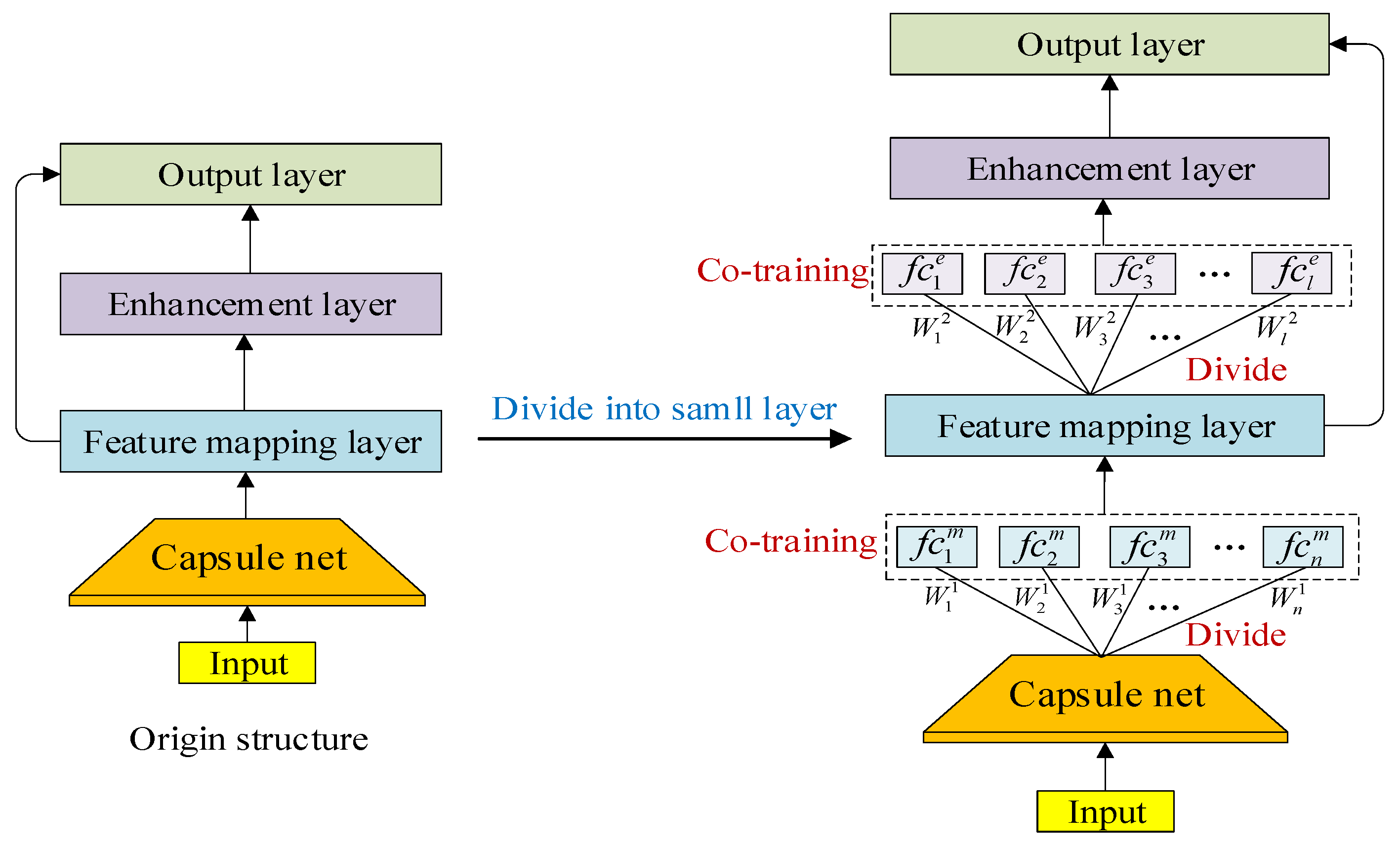
• The UDC framework: Implements a flexible feature filter through the UDC framework, which enhances feature extraction by segmenting fully connected layers into smaller, co-trainable units. Proven to improve recognition accuracy and operational efficiency over traditional CapsNet and BLS models.
• Enhanced learning via PS network: Features a PS network that promotes secondary learning by sharing weights and biases across BLS node layers, which boosts feature extraction and generalization capabilities. Includes a novel activation function, Uish, tailored for swift SAR classification, outperforming other deep learning models in comparative tests.
• Robustness and generalization: By leveraging the unique designs of the UDC framework and PS network, CBLS-SARNET demonstrates strong spatial feature extraction and adaptability under challenging conditions, including noise, blur, and varying depression angles, ensuring robust performance across diverse operational environments.

To validate the performance of CBLS-SARNET, this paper is structured as follows: Section 2 provides a review of the preliminary theory, Section 3 elaborates on the structure of CBLS-SARNET, Section 4 presents experimental analysis and validation of the proposed method, and Section 5 concludes this paper.

2. Preliminary

2.1. Challenges of CNN in SAR ATR

CNNs have been extensively utilized in SAR ATR with the rapid advancement of deep learning. CNNs exhibit satisfactory performance particularly when the test and training data of SAR images are closely aligned. Traditional CNNs, in contrast to perspective transformation, prioritize perspective invariance, which can be formulated as follows:

$$f\left(Tx\right)=f\left(x\right)$$

(1)

where T represents the direction of the target. Conventional CNNs, characterized by local connections and parameter sharing, do not adequately account for the positional relationships and connections among features.

Consequently, CNNs lack preserved spatial features. When SAR targets exhibit rotation or other directional variations, CNN performance diminishes. To accurately classify and identify SAR targets, maintaining images recognized from multiple viewpoints and orientations is crucial. Achieving translation invariance in CNNs requires enhancing model generalization through data augmentation, primarily addressing angle invariance via three perspective transformation methods: translation, rotation, and scaling [27].

However, adopting a perspective transformation may pose challenges. Firstly, it may hinder the network’s ability to distinguish between individual components and the whole. Secondly, excessive training data could lead to diminished model training efficiency. Therefore, if the network can effectively discern perspective transformation information, it would significantly enhance model generalization.

2.2. Basic Theory of CapsNet

In CapsNet, crucial information about all capsule detections, representing feature attributes, is encapsulated in the form of vectors. Capsules comprise nested collections of neural layers, wherein the modulus of the vector signifies the vector’s direction, attitude message, and the probability of the presence of target features. Broadly, CapsNet comprises three components: the convolutional layer, the PrimaryCaps layer, and the DigitalCaps layer.

The convolutional layer, constituting the initial segment of CapsNet, primarily extracts low-level features from images and converts pixels into activity vectors for local feature detection. Subsequently, the PrimaryCaps layer integrates the low-level features detected by the convolutional layer. Lastly, the DigitalCaps layer, consisting of three fully connected (FC) layers, corresponds to the actual experimental conditions, with this layer comprising g capsules representing g classes. Unlike traditional CNN scalar-to-scalar connections, the connection between PrimaryCaps and DigitalCaps entails vector-to-vector connections, which significantly enhances computational efficiency compared to pooling layer calculations.

2.3. Basic Theory of Broad Learning

The essence of BLS lies in finding the pseudo-inverse of feature and enhancement nodes to target values on a random vector functional link network [28,29]. The original BLS network is depicted in Figure 1a. Compared to a traditional model, this network is characterized by simplicity and ease of updating.

Suppose $A_n$ representing an n × m matrix, which is identical to inserting a novel column into the matrix $A_{n+1}^{+}$, is written as

$$A_{n+1}\underset{=}{{\displaystyle \Delta }}[A_n|a]$$

(2)

The matrix $A_{n+1}^{+}$ is equal to

$$\left[\begin{array}{c}{A}_n^{+}-d{b}^T\\ b^T\end{array}\right]$$

(3)

where $d=A_n^{+}a$,

$$b^T=\left\{\begin{array}{ll}{(c)}^{+}& if c\ne 0\\ {(1+d^{T}d)}^{-1}{d}^T{A}_n^{+}& if c=0\end{array}\right.$$

(4)

and $c=a-A_{n}d$. The weights are represented by

$$W_{n+1}=\left[\begin{array}{c}{W}_n-d{b}^T{Y}_n\\ b^T{Y}_n\end{array}\right]$$

(5)

where $W_n$ and $W_{n+1}$ stand for without and with new enhanced nodes, respectively. The pseudo-inverse $A_n^{+}$ and the weight $W_n$ will be updated rapidly with $A_n$. Figure 1b illustrates the network incorporating a novel node, where A denotes the input matrix. Subsequently, a dynamic system is established to update the model weight in real time for the newly added nodes. A still represents the input matrix. Utilizing ridge regression algorithms, this can be expressed as

$$W^m={(\lambda I+A{A}^T)}^{-1}{A}^{T}Y$$

(6)

Specifically, it can be written by

$$A^{+}=\lim {(\lambda I+A{A}^T)}^{-1}{A}^T$$

(7)

where $\lambda$ represents the constraints on the weights W derived from ridge regression algorithms.

2.4. Activation Function

The robustness and generalization of a neural network model are closely tied to the choice of activation function within the network. Selecting the appropriate activation function can enhance benchmarks, resulting in improved convergence. These nonlinear functions possess special properties that empower neural networks to capture complex features and yield significant outputs across various domains. General properties of activation functions include the following. Differentiability: ensuring gradients can be computed during optimization. Nonlinearity: the derivative typically varies, preventing the network from becoming a linear single-layer model. Simplicity: activation functions are usually relatively straightforward, as complexity may hinder computational speed. Saturation: Refers to intervals where gradients vanish, preventing further parameter updates; Monotonicity: signifies that the derivative’s sign remains consistent. A convex function is guaranteed for a single-layer network if the activation function is monotonic. Without an activation function, a network essentially reduces to a linear regression model capable of solving only linearly separable problems.

3. Method

In this part, we demonstrate the application of CBLS-SARNET in small-sample SAR ATR through theoretical analysis. Section 3.1 introduces the architecture of CBLS-SARNET. Section 3.2 introduces SAR image pre-processing. Section 3.3 proves the equivalence of our method. Section 3.4 presents the UDC framework. Finally, Section 3.5 introduces how to achieve fast SAR ATR through the PS network.

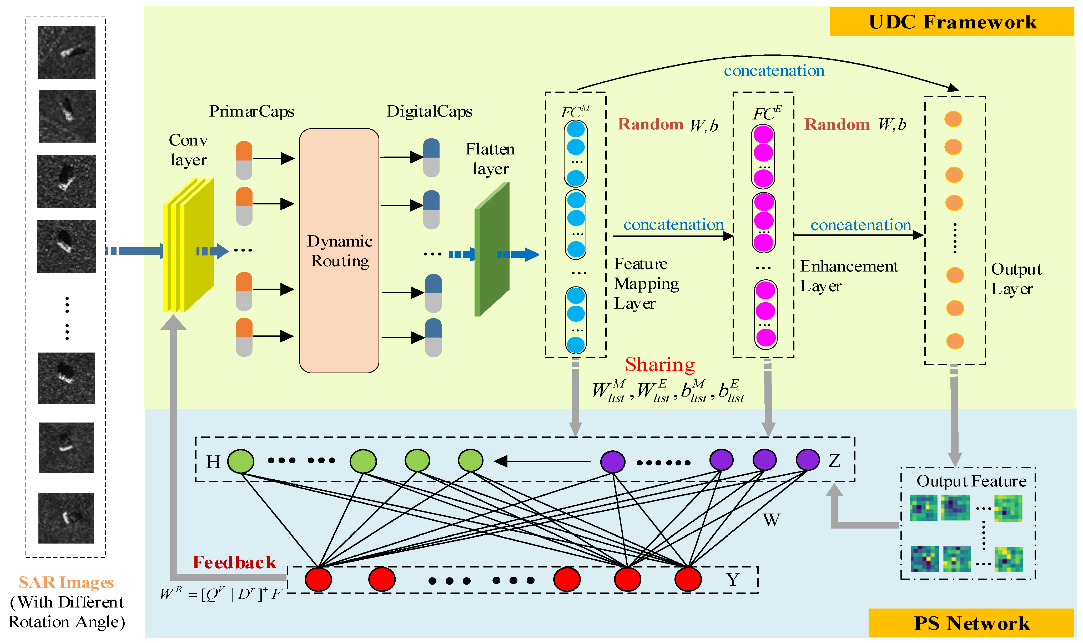
3.1. CBLS-SARNET Architecture

This paper introduces an effective and robust method, CBLS-SARNET, for addressing the SAR ATR problem with limited samples. Figure 2 illustrates the overall network architecture of this method. The design objective is to enhance the feature extraction capability of the network by selecting significant features through feature screening, eliminating irrelevant and redundant features, thereby achieving efficient target recognition for small samples in SAR images.

The method is divided into the UDC framework and the PS network. The UDC framework is designed similarly to BLS to achieve weight and bias sharing. The coefficients of BLS can be obtained through pseudo-inversion. However, it differs in that all components comprise FC layers for co-training. In the FC layer, each node is connected to all nodes in the preceding layer, facilitating the integration of features extracted from the front. Moreover, the learning process of these two layers adheres to the back-propagation theorem. This design aims to enhance the network’s feature extraction capabilities, as demonstrated by improvements in training speed and testing accuracy [30].

The PS network is adapted from the BLS structure. Nonetheless, the distinction lies in the pre-trained parameters of nodes. The network shares the pre-training weights with the UDC framework. The goal is to deeply extract spatial feature details, effectively guiding the network to extract vital image semantic information and robust features. Additionally, the PS network introduces a novel node activation function tailored to the characteristics of SAR images. Experimental results demonstrate that this proposed activation function enhances network performance compared to traditional activation functions.

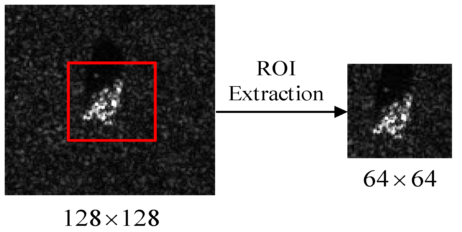
3.2. SAR Image Pre-Processing

Suppose that to extract Region Of Interest (ROI) from SAR target images, $B_1,B_{2,}\dots ,B_n$ are used, where the number of samples of the nth type is $B_n$, and the $j^{th}$ feature attribute of the nth type is $X_n^j$. The ROI feature extraction is performed, and the image centroid is calculated using

$$(x_c,y_c)=(\frac{m_{10}}{m_{00}},\frac{m_{01}}{m_{00}})$$

(8)

where $m_{10}$ and $m_{01}$ are the first-order original moments, $m_{00}$ is the original moments, and the center-of-mass coordinate is $(x_c,y_c)$. The ROI extraction process is shown in Figure 3.

3.3. From Invariance to Equivalence

To accurately identify SAR targets with various poses, it is crucial to preserve the hierarchical pose relationship between the whole object and its constituent parts. While traditional CNN methods excel at extracting texture, shape, and other object features, they often struggle to discern spatial transformations of objects, demonstrating limited translation invariance. However, CapsNet addresses this limitation by incorporating the relative spatial relationships between objects, representing them as pose matrices, known as “equivalence”.

To achieve equivalence, a precise representation of individual parts within the image is necessary. The manifold is associated with the presented parts, with perspective transformations resulting in slight changes in the poses of these parts. Therefore, the image undergoes initial processing by the CNN, and the feature vector is transformed into the shape of $H^{\prime }\times W^{\prime }\times C\mathrm{apsule}Dim$. This step aims to encapsulate image component information into the learned manifold. A vector that stores part pose and presentation probability information is called a capsule. The pose matrix employs a weight matrix to depict the relationship between the part and the overall pose. Given the pose vector $p_e$ of the component, the corresponding overall pose $p_f$ of the target can be expressed as

$$p_e\cdot W_{ef}=p_f\iff f(p_e)=p_f$$

(9)

The object is transformed as a whole part. Due to the equivalence of the viewing angle, there are

$$(C{p}_e)\cdot W_{ef}=C{p}_f$$

(10)

Further, transforming it will obtain

$$f(C{p}_e)=Cf(p_e)\iff f(Cx)=Cf(x)$$

(11)

where C is a constant coefficient. By accurately representing the components and leveraging the perspective equivalence of the whole-component relationship, the perspective-equivalent transformation method is derived.

3.4. Feature Screening via UDC Framework

Redundant features can lead to risks such as model overfitting. To mitigate issues stemming from an excessive number of features, feature filtering becomes imperative. Hence, the UDC framework is designed as a feature filter incorporating various perspectives. When confronted with high-dimensional features, the UDC framework exhibits superior robustness and can implicitly select features to eliminate irrelevant and redundant ones. Feature screening can be conceptualized as a trained neural network model M. Given a sample w, it can be interpreted as a sequence of several features $(w_1,w_2,w_3,\dots )$. Utilizing the feature sensitivity analysis method based on the receptive field, the contribution of each feature to a specific neural network category, such as the predicted probability $p_{\stackrel{⌢}{y}}$ of the true sample category $\stackrel{⌢}{y}$, can be obtained from $[im{p}_{w_1},im{p}_{w_2},im{p}_{w_3},\dots ]$, and then the average contribution of each feature when it appears is

$$im{p}_{w_i}=\frac{1}{N}{\displaystyle \sum _{j\in doc(w_i)}im{p}_{w_{ij}}}$$

(12)

where $im{p}_{w_{ij}}$ represents the contribution of feature i in sample j.

The feature screening mechanism of the UDC framework is implemented through network co-training. Co-training is a divergence-based approach that assumes each sample can be feature-extracted from a different perspective. Various feature filters can be trained from distinct views and then the features deemed credible to join the network can be selected. As these feature filters are trained from diverse perspectives, they can complement each other and enhance the recognition rate. This aids in sifting through information and reducing redundant features, much like gaining a better understanding of things from different perspectives. The UDC framework is illustrated in Figure 4.

Supposing that T training samples $X={\left\{{\mathrm{x}}_t\right\}}_{t=1}^T$ from the C class, cross-entropy can be calculated as

$$f_{loss}(p,y)=-\frac{1}{T}{\displaystyle \sum _{t=1}^T{\displaystyle \sum _{c=1}^C{y}_{n,c}\log (O_{n,c})}}$$

(13)

Among them, $y\in \{0,1\}$ refers to the true label and $O\in [0,1]$ stands for the softmax normalized probability generated from the training model.

Assume that the feature mapping layer M is divided into m smaller layers. Due to its fully connected characteristics, the FC layer contains numerous parameters. In this process, the entire FC layer is partitioned into several smaller FC layers to facilitate different layer co-training, resulting in a significant reduction in network computation [31]. Some splitting methods [32] use an implicit “divide and ensemble” strategy. By adhering to the principles of maintaining metrics, the number of parameters remains roughly unchanged regardless of whether division is employed or not.

According to the definition in PyTorch, $K\times K$ represents the size of its kernel. $C_{in}$ and $C_{out}$ represent the input and output maps, which stand for the number of feature maps with d as the group quantity and represent every input channel $C_{in}/d$ that is convolved with their sets of filters of size $C_{out}/d$. Under this situation, the parameters’ quantity is $(K^2\times C_{in}\times C_{out})/d$ and the floating-point operations are $(2\times K^2\times (C_{in}/d)-1)\times H\times W\times C_{out}$, where $H\times W$ shows the output feature map size and −1 appears after adding $((K^2\times C_{in})/d)$ numbers, which only need $((C_{in}\times K^2)/d)-1$ operations. The omission of the bias serves for brevity. In depthwise convolution, we have $d=C_{in}$. Commonly,

$$C_{out}=t_1\times C_{in}$$

(14)

in which t₁ serves as a constant. Therefore, an FC layer needs to be divided by a factor S, dividing C_in by $\sqrt{S}$, which can fully achieve the goal:

$$\frac{K^2\times C_{in}\times C_{out}}{S}\times \frac{1}{d}=K^2\times t_1\times {(\frac{C_{in}}{\sqrt{S}})}^2\times \frac{1}{d}$$

(15)

After division, different angles of the same samples are utilized for co-training [33], aiming to train small connection layers to enhance the diversity of features and achieve better integration properties. Simultaneously, network learning can occur among small connection layers to further enhance individual performance.

If a given SAR feature vector $X=\{x_1,x_2,\dots ,x_N\}$ contains N samples that were operated after CapsNet, each sample has M dimensions. For n layers of feature mapping layers division, l layers of enhancement layers are given. The input feature vector X is projected and the $i^{th}$ mapping feature vector can be expressed as

$$Z_i^m=\phi (X{W}_i^1+b_i^m)$$

(16)

where $W_i^1$ and $b_i$ represent the weight and bias of the feature mapping layer $f{c}_i^m$. And ${\left\{Z_i\right\}}_{i=1}^m$, $i=1,2,\dots ,n$, $\phi (\cdot )$, is an optional nonlinear activation function. All feature mapping layers can be denoted as $F{C}^M=\{f{c}_1^m,f{c}_2^m,\dots ,f{c}_n^m\}$, which will be co-training at the same time.

After division, the weight and bias of the feature mapping layer can be written as $W_{list}^M=[W_1^1,W_2^1,\dots ,W_n^1]$ and $b_{list}^M=[b_1^m,b_2^m,\dots ,b_n^m]$. Similarly, the $j^{th}$ group of enhancement nodes can be written as

$$H_j^e\equiv \xi (Z_i^m{W}_j^2+b_j^e)$$

(17)

where $W_j^2$ and $b_j$, respectively, represent the weight and bias of the enhancement layer $f{c}_j^e$. And ${\left\{H_j\right\}}_j^e$, $j=1,2,\dots ,l$. $\xi (\cdot )$ refers to a nonlinear activation function. With the same calculation, all enhancement layers can be represented as $F{C}^E=\{f{c}_1^e,f{c}_2^e,\dots ,f{c}_l^e\}$, which will be training together for reducing the occupation of computing resources.

Furthermore, the weight and bias of enhancement layers can be written as $W_{list}^E=[W_1^e,W_2^e,\dots ,W_l^e]$ and $b_{list}^E=[b_1^e,b_2^e,\dots ,b_l^e]$.

Lastly, the feature mapping and the enhancement layer are concatenated together and fed into the output layer, inspired by [34], which proves that the weight will efficiently improve performance during training and maintain the efficiency of inference. The output layer can be described as

$$f_{output}=\sigma (F{C}^M+F{C}^E)$$

(18)

where $\sigma$ denotes the nonlinear function.

3.5. Fast SAR ATR Task via PS Network

3.5.1. PS Network

The PS network fully leverages the advantages of the BLS network. The weights and biases of the feature and enhancement nodes in the PS network are shared with the UDC framework for fast fine-tuning, drawing inspiration from the parameter-sharing concept in transfer learning [35]. Transfer learning addresses issues such as overfitting and local optima resulting from limited training samples [36]. Unlike traditional transfer learning, the PS network does not differentiate between target and source domains. Instead, it solely shares pre-training weights and biases with the UDC framework, enabling the extraction of deeper semantics from images through secondary learning. This design facilitates the network’s ability to uncover SAR features from secondary learning, enhancing network robustness.

The PS network requires mapping features into a feature space and finding a metric within that space to minimize the difference between the feature distributions of pre-training and prediction data. Define that x is an instance set and $\mathbb{Z}$ represents a feature space.

Suppose that $D_s$ is the pre-training data distribution defined on x, $D_s^{\prime }$ is the pre-training feature distribution defined on $\mathbb{Z}$, and $D_T$ and $D_T^{\prime }$ also represent the predicted data distribution and feature distribution, respectively. $\Re$ is the representation function that maps the instance x on $\mathbb{Z}$. f is the true label function, which needs to be trained. h is the prediction function, $h\in H$. When given a feature z to h, it will acquire the corresponding label. Therefore, the real mapping function can be obtained as

$$f^{\prime }(z)\stackrel{def}{=}{E}_{x~D_S^{\prime }}[f(x)|R(x)=z]$$

(19)

The error rate of the prediction function h on the pre-training data is

$${\epsilon }_S(h)=E_{z~D_S^{\prime }}|f^{\prime }(z)-h(z)|$$

(20)

which measures the distance between feature distributions $D_s^{\prime }$, and $D_T^{\prime }$ is mapped to the feature space by $\Re$. The condition of this distance is that it can be calculated by limited sample data. The metric can be designed as

$$d_{\gamma }(D_S^{\prime },D_T^{\prime })=2\underset{A\in \gamma }{\sup }|{\mathrm{Pr}}_{D_S^{\prime }}[A]-{\mathrm{Pr}}_{D_T^{\prime }}[A]|$$

(21)

where $D_s^{\prime }$ is a subset and represents the distance. $D_s^{\prime }$ represents traversing all subsets of $D_s^{\prime }$ to find the maximum probability difference between $D_s^{\prime }$ and $D_T^{\prime }$.

The UDC framework is supposed to obtain $[W_{list}^M|b_{list}^M]$ and $[W_{list}^E|b_{list}^E]$, which represents the way to learn the SAR images feature.

For v mapping features, the r enhancement nodes are given. Feature nodes can be expressed as $Q=\psi (f_{output}{W}_{list}^M+b_{list}^M)$ and enhancement nodes can be expressed as $D=\zeta (Q^v{W}_{list}^E+b_{list}^E)$. $\psi (\cdot )$ and $\zeta (\cdot )$ are set to Uish, which is a novel activation function designed for the PS network.

The combined matrix acquired by interfacing both enhancement nodes and feature nodes is regarded as the actual contribution of the framework, with an output matrix of $F\in R$, and this network can be obtained by

$$\begin{array}{l}F=[Q_1,\dots ,Q_v|\xi (Q^V{W}_{list}^E+b_{list}^E),\dots ,\xi (Q^V{W}_{list}^E+b_{list}^E)]W^R\\ =[Q_1,\dots ,Q_v|D_1,\dots ,D_r]W^R\\ =[Q^V|D^R]W^R\end{array}$$

(22)

Equation (22) can be shortened as $F=[Q^V|D^R]W^R$. According to (6) and (7), we have $A^{+}={[Q^V|D^r]}^{+}$. Therefore, $W^R={[Q^V|D^r]}^{+}F$ is the connection weight of this network.

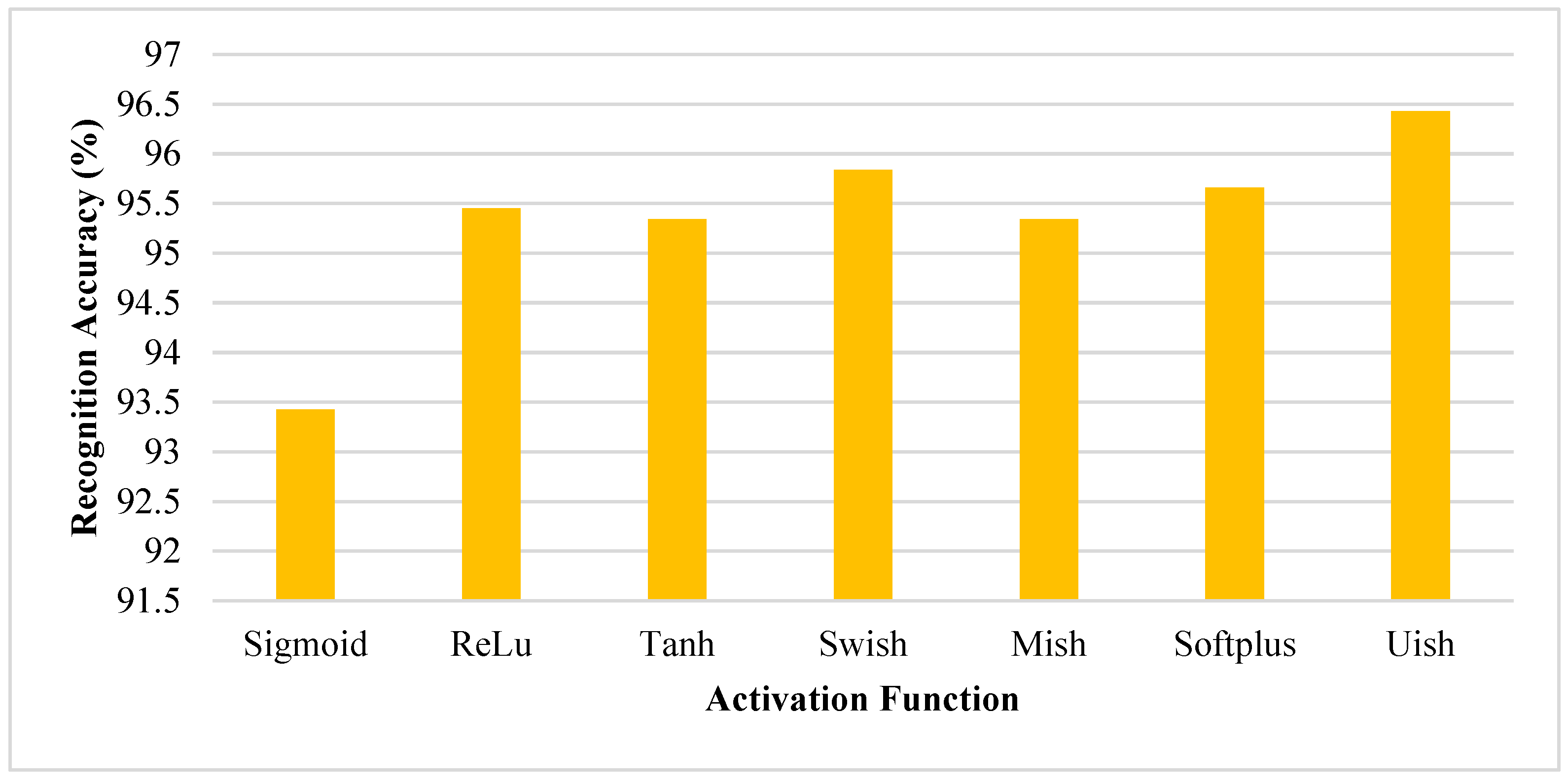
3.5.2. Uish Function

In CBLS-SARNET, the activation function serves to provide the nonlinear modeling capability essential for ensuring the network’s reliability and optimizing its overall performance. Moreover, given the uncertainty inherent in SAR ATR samples, it becomes necessary to dynamically adjust the network’s activation function settings. Algorithm 1 lists the pseudo-code of the overall process of CBLS-SARNET.

Algorithm 1: Pseudo-code of CBLS-SARNET

To address this need, a novel activation function called Uish is proposed. Uish satisfies the general properties expected of an activation function. Its mathematical formula is relatively simple, thereby reducing computational complexity. The Uish function is mathematically defined as

$$f(x)=kx\cdot \mathrm{softplus}(x)$$

(23)

where $\mathrm{softplus}(x)=\log (1+e^x)$. Moreover, x represents the input to the neuron and k is a variable coefficient.

In fact, like other activation functions, Uish is unbounded above and bounded below. It can be seen as a smoothing of the ReLU function, which is also non-monotonic in gradient and smoothing. As the value of k increases, the function curve becomes steeper, resulting in a faster growth rate. The first derivative of Uish is also unbounded above and bounded below. When k > 0, it is smooth and monotonic. Furthermore, the monotonicity property of Uish resembles that of the most common activation functions, making it continuously differentiable. The derivative of Uish is

$$f^{\prime }(x)={[kx\cdot \mathrm{softplus}(x)]}^{\prime }=k\cdot [\log (1+e^x)+x\frac{e^x}{1+e^x}]$$

(24)

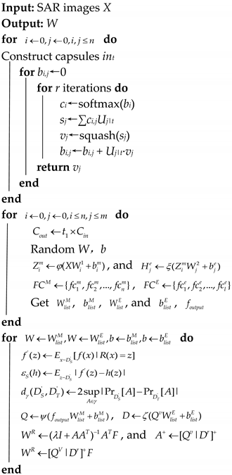
4. Experimental Results and Analysis

We experimentally verify the performance of CBLS-SARNET in this section. All experiments were conducted using the PyTorch platform on an NVIDIA GTX2070 8G GPU, utilizing the Moving and Stationary Target Acquisition and Recognition (MSTAR) dataset. It is noteworthy that the CBLS-SARNET does not rely on data augmentation.

4.1. Dataset Distribution

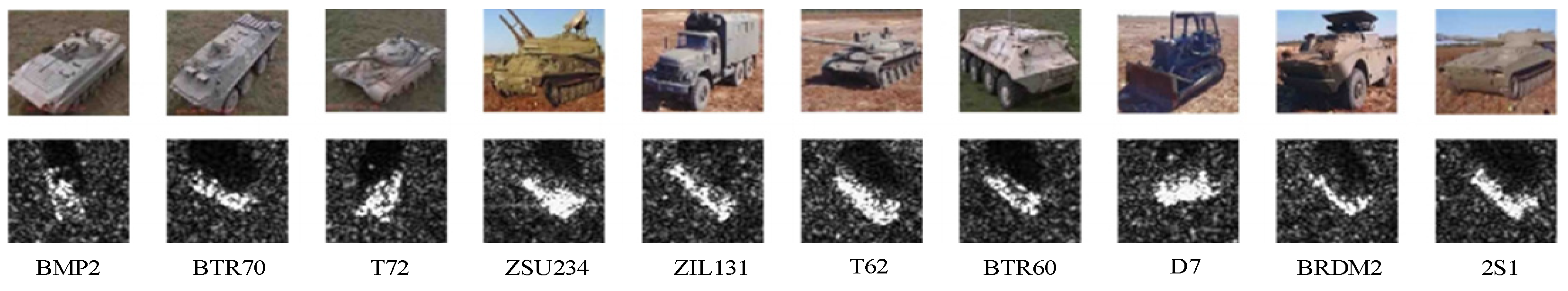
4.1.1. MSTAR Datasets

The MSTAR datasets utilize the measured SAR ground stationary target data released by the MSTAR program. To eliminate redundant backgrounds in the images, all SAR images in the experiments are cropped into regions of interest (ROIs) with dimensions of 64×64 pixels. The dataset includes ten types of targets, as shown in Figure 5.

In the Standard Operating Conditions (SOCs), each type in the MSTAR datasets contains depression angles $17°$ and $15°$, which is listed in

Table 1. The distribution of SOC MSTAR datasets.

Target	Training Datasets		Test Datasets
	Depre.	Number	Depre.	Number
BMP2	17°	233	15°	587
BTR70		233		196
T72		232		582
ZSU23/4		299		274
ZIL131		299		274
T62		299		273
BTR60		256		195
D7		299		274
BDRM2		298		274
2S1		299		274
Total		2747		3203

. The SOC refers to the slight change in sensor depression angle and no target occlusion.

The Extended Operating Condition (EOC) MSTAR datasets are listed in

Table 2. The distribution of EOC MSTAR datasets.

Dataset	Depre.	2S1	BDRM2	ZSU23/4	Total
Training dataset	17°	299	298	299	896
Test dataset	30°	288	287	288	863
	45°	303	303	303	909

. Compared with the SOC, the EOC refers to the large change in depression angle of the sensor, the existence of multiple target configurations, target concealment, and camouflage, which include depression angles ${30}^{°}$ and ${45}^{°}$. Since the EOC has angles of different scales, it is used to test the sensitivity of the CBLS-SARNET to the rotation angle of SAR images.

4.1.2. SOC Small-Sample Datasets

The SOC small-sample datasets mainly aim to divide the training set of the database by the proportions of 1:32, 1:16, 1:08, 1:04, 1:03, and 1:02 based on the SOC. We set depression angle $17°$ as the training set and depression angle $15°$ as the test set.

4.1.3. EOC Small-Sample Datasets

To gain a deeper understanding of the network robustness, an experiment is set-up with large depression angle changes in the EOC, including depression angles $30°$ and $45°$ for testing and depression angle $17°$ for training. This is mainly to divide the training set of the datasets by the proportions of 1:32, 1:16, 1:08, 1:04, 1:03, and 1:02.

4.2. Experimental Setup

In this section, all test settings are based on a ratio of 1:02 in the SOC small-sample datasets. To achieve a better performance of CBLS-SARNET, various hyperparameters, including feature nodes and enhancement nodes, batch size, capsule number, learning rate, training epochs, and the optimizer, are tested in a suitable experimental manner. More specifically, the experimental settings are listed in

Table 3. Parameter setting of CBLS-SARNET.

Parameters	Setting
Feature nodes	500
Enhancement nodes	500
Batch sizes	128
Capsule number	8
Learning rate	0.0003
Epochs	300
Optimizer	Adam

.

In our experiments, the reported recognition rates represent the average recognition rate across different target types included in the MSTAR dataset. These averages provide a general measure of the model’s performance across the varied scenarios presented by this dataset.

4.3. Activation Function Verification

To verify the effectiveness of Uish, we demonstrate its properties from simplicity and robustness. The experimental setup is based on Table 3.

The recognition accuracies reported in Figure 6 are indeed the highest achieved accuracies for each activation function during our experiments. To obtain these results, multiple runs are conducted for each activation function to mitigate any anomalies due to random initialization and to ensure the robustness of the findings. The presented data are the average of these runs, reflecting the most consistent high-performance outcomes for each activation function.

First, we examine the Uish performance under different coefficient values of k on the SOC small-sample dataset of 1:02 to determine the optimal coefficient setting range for Uish performance. Second, we compare the performance of Uish with those of different baseline activation functions using the same network architecture while keeping other training parameters unchanged.

The compared activation functions include Sigmoid, ReLU, Tanh, Swish, Mish, and SoftPlus. For all experiments in this section, only the activation function is changed while all other settings remain unchanged.

Table 4. The recognition accuracy of Uish under different coefficient values k.

k	Accuracy (%)	k	Accuracy (%)
1	90.23	0.1	95.64
0.1	95.98	0.2	96.01
0.001	94.32	0.3	98.34
0.0001	96.79	0.4	95.98

shows that as the value of k changes, the recognition accuracy also varies. The bold font indicates the highest recognition accuracy in this experimental table. Among them, when the k value is set to 0.3, the recognition result is better than those of other k values. This proves the gradient-based optimization network is more stable when the output value of Uish is limited.

Furthermore, Figure 6 illustrates the recognition results of CBLS-SARNET under various activation functions. It is observed that Uish outperforms other activation functions with the highest recognition rate, showcasing its strong performance.

4.4. Equivalence Verification Experiment of CBLS-SARNET

When the depression angle is changed, SAR images exhibit significant differences. To further exploit the equivalence of the CBLS-SARNET, we conducted experiments under different depression angles and compared them with seven other deep learning methods. They are Xception [37], Inceptionv3 [38], DenseNet [39], VGG [40], ResNet [41], LeNet [42], and AlexNet [43]. These deep learning methods possess powerful feature extraction capabilities and have made significant advancements in image recognition, which can effectively validate the performance of CBLS-SARNET.

This experiment is validated and analyzed on EOC small-sample datasets. As the results displayed in Figure 7, CBLS-SARNET far exceeds other advanced deep learning methods at depressions $30°$ and $45°$. This is attributed to the spatial feature extraction capability of CBLS-SARNET, which can retain more useful spatial features compared to traditional CNNs when the SAR targets have varying depression angles. The rotational samples are analyzed through multiple capsules trained to perceive differently. Each attribute in the SAR images from different depression angles is represented by a vector. Overall, the experimental results demonstrate that CBLS-SARNET exhibits equivalence properties when depression angles vary within a small range.

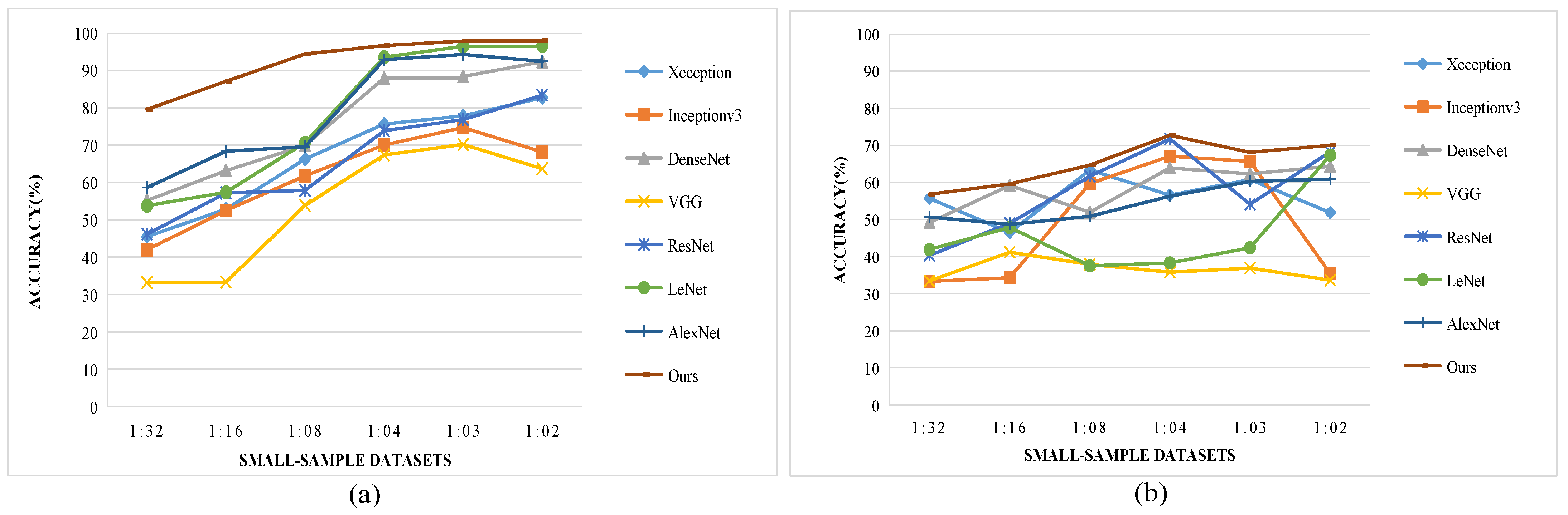
4.5. Generalization and Robustness of CBLS-SARNET

For a thorough exploration of CBLS-SARNET’s performance, experiments are conducted by introducing Gaussian blur, Gaussian noise, and noisy labels to the SOC small-sample datasets.

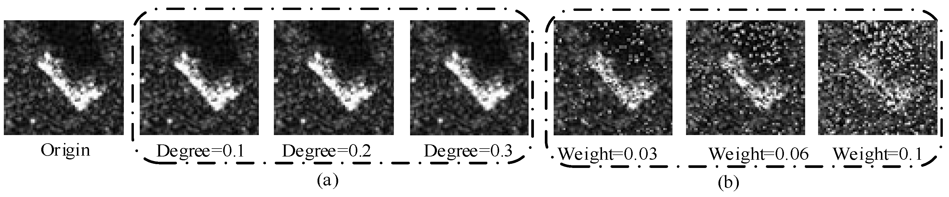
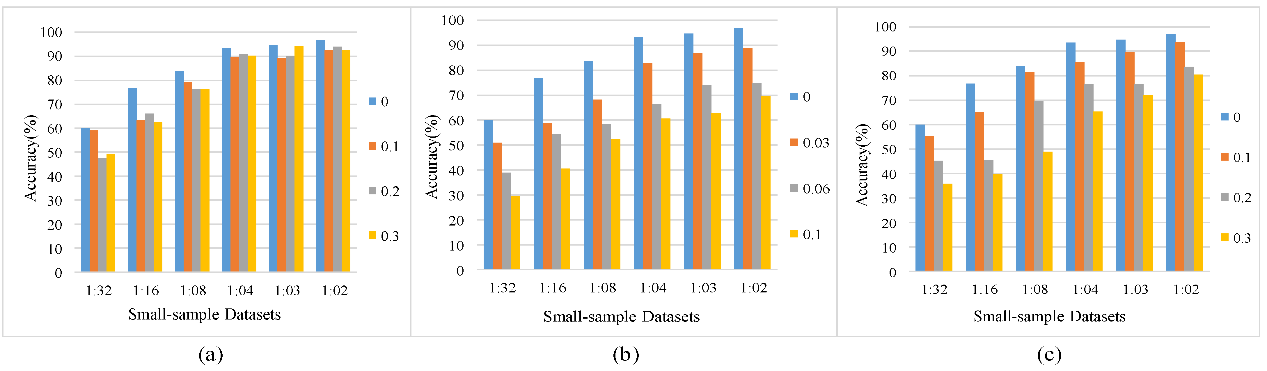
4.5.1. Blur Analysis

In this experiment, we applied Gaussian blur to SAR images. Figure 8a displays the SAR images after adding different levels of blur, where $\delta$ represents the degree of Gaussian blur. When $\delta$ set to 0, Gaussian blur is not added. When the range is set to 0.1 to 0.3, the blur degree ranges from 0.1 to 0.3. Figure 9a demonstrates that with the increase in blur, the impact on the model is minimal. In conclusion, the experiment illustrates that the CBLS-SARNET can still maintain a robust feature extraction capability for SAR images, even though increasing blur may obscure the features of SAR images.

4.5.2. Noise Analysis

The SAR images are affected by coherent signals generated from scattered echoes of ground objects, often resulting in noise. To investigate this, we conducted experiments under various conditions of Gaussian noise. Similar to speckle noise, Gaussian noise can disrupt network information acquisition. When $\varphi$ is set to 0, it denotes that Gaussian noise is not added. And the weight $\varphi$ of noise ranges from 0.03 to 0.1. Figure 8b shows the SAR images after adding Gaussian noise. From Figure 9b, it is evident that increasing noise levels have minimal impact on model performance. Analysis of the recognition results demonstrates that despite a decrease in accuracy after introducing Gaussian noise, it remains within an acceptable range. We defined the lower limit of this range as about a 40% drop from the baseline accuracy achieved without noise. We speculate that CBLS-SARNET exhibits robust noise discrimination capabilities in SAR images, enabling the retention of useful features during the recognition process.

4.5.3. Noisy Labels Analysis

The inevitable presence of noisy labels poses challenges to SAR ATR in practical applications. Therefore, an experiment was designed to assess CBLS-SARNET. The experiment varied the degree of noisy labels from 0 to 0.3 for small-sample datasets. A degree of 0 indicates no noisy labels. The results, depicted in Figure 9c, illustrate that CBLS-SARNET can effectively mitigate the impact within a range of noisy label degrees from 0.1 to 0.2. However, its performance diminishes at a degree of 0.3 compared to the former two degrees. Particularly for datasets with a ratio of 1:32, the network is most affected by noisy labels, leading to a slight drop in recognition rate. This is attributed to the dataset’s small size, resulting in a higher proportion of noisy labels. While our method may not effectively handle SAR datasets with a large proportion of noisy labels, it demonstrates robust generalization when dealing with datasets containing only a small number of noisy labels.

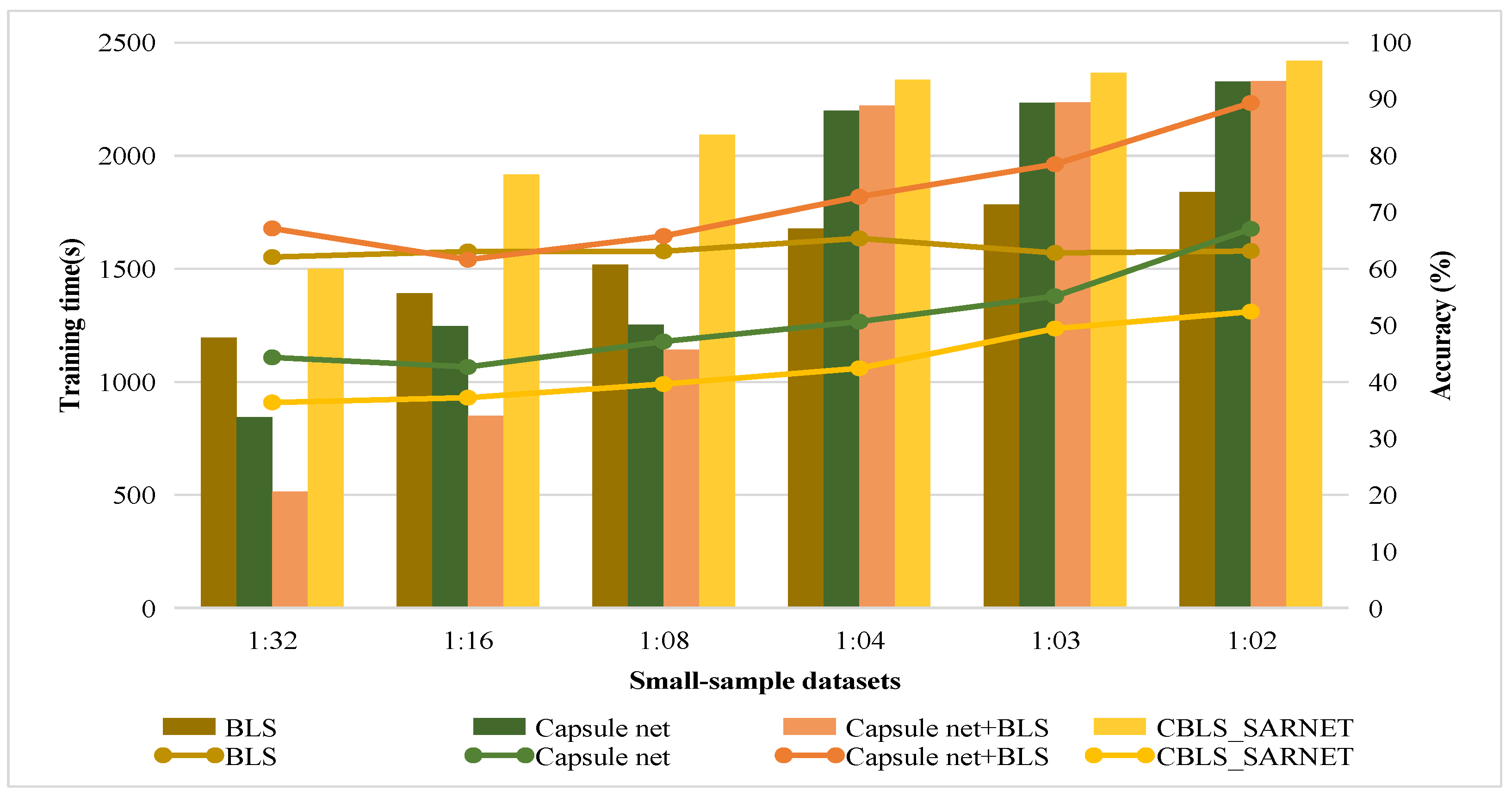
4.6. Efficiency and Effectiveness of CBLS-SARNET

4.6.1. Efficiency Verification

We conduct a comparative analysis between CBLS-SARNET, BLS, CapsNet, and ‘CapsNet + BLS’ in terms of recognition accuracy and training time. Here, ‘CapsNet + BLS’ denotes a configuration where CapsNet and BLS are not connected in an end-to-end manner, serving as a point of contrast with CBLS-SARNET. The experiments are conducted using SOC small-sample datasets, and the experimental configurations are shown in Table 3.

Figure 10 illustrates the recognition accuracy and training time of each model. The line graph represents the corresponding training times, while the histogram depicts the recognition accuracy achieved by each model. Our experimental findings demonstrate that CBLS-SARNET exhibits the shortest training time while maintaining the highest recognition accuracy among the tested methods.

4.6.2. Effectiveness Verification

We conduct a comparison between CBLS-SARNET and nine popular deep learning methodologies to assess their recognition performance [44,45]. These networks are A-ConvNets [46], CNN-TL [3], Xception, DenseNet, Inceptionv3, ResNet50, VGG, AlexNet, and LeNet. A-ConvNets solely comprise sparsely connected layers, which effectively reduce parameters while achieving commendable SAR ATR results. Additionally, CNN-TL leverages transfer learning, enabling the training of knowledge obtained from unlabeled SAR images to labeled target images. This approach has demonstrated improved network training performance, even with limited SAR data.

Given that these deep learning methods are constructed upon different structural principles, we adopt recognition accuracy as the benchmark metric for comparative analysis across identical datasets. Our experiments are conducted using SOC small-sample datasets, with experimental configurations set according to the parameters outlined in Table 3. Recognition results under varying small-sample dataset proportions are tabulated in

Table 5. Recognition accuracy (%) with different deep learning methods.

Method	1:32	1:16	1:08	1:04	1:03	1:02
VGG	14.00	31.40	39.20	46.10	55.50	62.40
InceptionV3	17.70	43.50	49.80	60.20	71.10	82.02
DenseNet	17.00	50.00	60.00	82.00	87.50	84.20
ResNet50	20.10	25.10	28.50	35.60	59.70	69.00
Xception	22.50	34.10	41.60	70.40	78.50	84.00
LeNet	31.60	48.00	63.00	80.90	84.10	87.40
AlexNet	38.20	60.50	80.90	89.70	92.40	93.20
CNN-TL	52.33	61.47	71.42	84.38	89.45	91.13
A-ConvNets	63.54	72.12	76.80	88.73	87.23	94.38
CBLS-SARNET	68.05	80.70	86.77	94.48	96.06	98.78

. Notably, our method demonstrates superior performance among supervised methods. The bold font indicates the highest recognition accuracy in this experimental table.

As can be seen from Table 5, CBLS-SARNET outperforms other deep learning methodologies across small-sample datasets at ratios of 1:32, 1:16, 1:08, 1:04, and 1:02. Even in datasets with a ratio of 1:32, containing up to nine samples per category, CBLS-SARNET achieves a recognition accuracy of 68.05%, surpassing A-ConvNets by 4.51%. Moreover, excluding the 1:32 dataset, CBLS-SARNET consistently outperforms popular deep learning networks in recognition accuracy across other dataset proportions. These experimental findings collectively prove the effectiveness of CBLS-SARNET in achieving robust performance.

In addition, we observed differences in performance based on the different types of targets. Factors contributing to these differences include the target’s size, shape, and the degree to which it blends into the surrounding clutter. Some targets, due to their distinct features and larger size, were recognized with higher accuracy compared to others that might have more complex or camouflaged appearances.

5. Conclusions

In this paper, a network named CBLS-SARNET is proposed, primarily amalgamating CapsNet and BLS through end-to-end co-training to address practical classification issues for small samples in SAR ATR. This method stands as an efficacious and efficient network due to its swift training capability and precise feature extraction, surpassing many sophisticated deep learning methods. The UDC framework, serving as a feature filter and pre-training structure, effectively enhances the spatial information acquisition ability and model iteration speed. The PS network facilitates secondary learning through weight and bias sharing, deepening the model’s comprehension of SAR targets. Experimental results validate CBLS-SARNET’s commendable performance in classification accuracy and training speed with limited data. Moreover, even in the presence of noise, blur, noisy labels, and larger depression angles, this method exhibits robustness and generalization.

In the future, we will investigate automated mechanisms for data augmentation to improve the robustness of the model against even more diverse operational scenarios. This includes implementing generative adversarial networks (GANs) to synthesize realistic training data under various conditions. By addressing these future challenges, we hope to extend the utility of CBLS-SARNET, making it a more versatile tool in the field of machine learning and image recognition.

References

1. Zhang, C.; Dong, H.; Deng, B. Improving Pre-Training and Fine-Tuning for Few-Shot SAR Automatic Target Recognition. Remote Sens. 2023, 15, 1709. [Google Scholar] [CrossRef]
2. Wang, C.; Shi, J.; Zhou, Y.; Li, L.; Yang, X.; Zhang, T.; Wei, S.; Zhang, X.; Tao, C. Label Noise Modeling and Correction via Loss Curve Fitting for SAR ATR. IEEE Trans. Geosci. Remote Sens. 2022, 60, 5216210. [Google Scholar] [CrossRef]
3. Zhu, M.; Cheng, J.; Lei, T.; Feng, Z.; Zhou, X.; Liu, Y.; Chen, Z. C-RISE: A Post-Hoc Interpretation Method of Black-Box Models for SAR ATR. Remote Sens. 2023, 15, 3103. [Google Scholar] [CrossRef]
4. Zhou, X.; Tang, T.; Cui, Y.; Zhang, L.; Kuang, G. Novel Loss Function in CNN for Small Sample Target Recognition in SAR Images. IEEE Geosci. Remote Sens. Lett. 2022, 19, 4018305. [Google Scholar] [CrossRef]
5. Li, Y.; Liu, W.; Qi, R. Multilevel Pyramid Feature Extraction and Task Decoupling Network for SAR Ship Detection. IEEE J. Sel. Top. Appl. Earth Obs. Remote Sens. 2024, 17, 3560–3570. [Google Scholar] [CrossRef]
6. Cao, C.; Cao, Z.; Cui, Z. LDGAN: A Synthetic Aperture Radar Image Generation Method for Automatic Target Recognition. IEEE Trans. Geosci. Remote Sens. 2020, 58, 3495–3508. [Google Scholar] [CrossRef]
7. Inkawhich, N.A.; Davis, E.K.; Inkawhich, M.J.; Majumder, U.K.; Chen, Y. Training SAR-ATR Models for Reliable Operation in Open-World Environments. IEEE J. Sel. Top. Appl. Earth Obs. Remote Sens. 2021, 14, 3954–3966. [Google Scholar] [CrossRef]
8. Sun, Y.; Wang, Y.; Liu, H.; Wang, N.; Wang, J. SAR Target Recognition with Limited Training Data Based on Angular Rotation Generative Network. IEEE Geosci. Remote Sens. Lett. 2020, 17, 1928–1932. [Google Scholar] [CrossRef]
9. Molini, A.B.; Valsesia, D.; Fracastoro, G.; Magli, E. Speckle2Void: Deep Self-Supervised SAR Despeckling with Blind-Spot Convolutional Neural Networks. IEEE Trans. Geosci. Remote Sens. 2022, 60, 5204017. [Google Scholar] [CrossRef]
10. Gao, G.; Liu, L.; Zhao, L.; Shi, G.; Kuang, G. An Adaptive and Fast CFAR Algorithm Based on Automatic Censoring for Target Detection in High-Resolution SAR Images. IEEE Trans. Geosci. Remote Sens. 2009, 47, 1685–1697. [Google Scholar] [CrossRef]
11. Li, Z.; Li, E.; Samat, A.; Xu, T.; Liu, W.; Zhu, Y. An Object-Oriented CNN Model Based on Improved Superpixel Segmentation for High-Resolution Remote Sensing Image Classification. IEEE J. Sel. Top. Appl. Earth Obs. Remote Sens. 2022, 15, 4782–4796. [Google Scholar] [CrossRef]
12. Zhang, P.; Tang, J.; Zhong, H.; Ning, M.; Liu, D.; Wu, K. Self-Trained Target Detection of Radar and Sonar Images Using Automatic Deep Learning. IEEE Trans. Geosci. Remote Sens. 2022, 60, 4701914. [Google Scholar] [CrossRef]
13. Ding, X.; Wang, N.; Gao, X.; Li, J.; Wang, X.; Liu, T. Group Feedback Capsule Network. IEEE Trans. Image Process. 2020, 29, 6789–6799. [Google Scholar] [CrossRef]
14. Sabour, S.; Frosst, N.; Hinton, G.E. Dynamic Routing Between Capsules. In Proceedings of the Advances in Neural Information Processing Systems; Guyon, I., Luxburg, U.V., Bengio, S., Wallach, H., Fergus, R., Vishwanathan, S., Garnett, R., Eds.; Curran Associates, Inc.: Long Beach, CA, USA, 2017. [Google Scholar]
15. Huang, R.; Li, J.; Wang, S.; Li, G.; Li, W. A Robust Weight-Shared Capsule Network for Intelligent Machinery Fault Diagnosis. IEEE Trans. Ind. Inform. 2020, 16, 6466–6475. [Google Scholar] [CrossRef]
16. Gong, Z.; Zhong, P.; Yu, Y.; Hu, W. Diversity-Promoting Deep Structural Metric Learning for Remote Sensing Scene Classification. IEEE Trans. Geosci. Remote Sens. 2018, 56, 371–390. [Google Scholar] [CrossRef]
17. Zhang, W.; Tan, Z.; Lv, Q.; Li, J.; Zhu, B.; Liu, Y. An Efficient Hybrid CNN-Transformer Approach for Remote Sensing Super-Resolution. Remote Sens. 2024, 16, 880. [Google Scholar] [CrossRef]
18. Xie, S.; Girshick, R.; Dollár, P.; Tu, Z.; He, K. Aggregated Residual Transformations for Deep Neural Networks. In Proceedings of the 2017 IEEE Conference on Computer Vision and Pattern Recognition (CVPR), Honolulu, HI, USA, 21–26 July 2017. [Google Scholar] [CrossRef]
19. Zhang, L.; Li, J.; Lu, G.; Shen, P.; Bennamoun, M.; Shah, S.A.A.; Miao, Q.; Zhu, G.; Li, P.; Lu, X. Analysis and Variants of Broad Learning System. IEEE Trans. Syst. Man Cybern. Syst. 2022, 52, 334–344. [Google Scholar] [CrossRef]
20. Chen, C.L.P.; Liu, Z. Broad Learning System: An Effective and Efficient Incremental Learning System without the Need for Deep Architecture. IEEE Trans. Neural Netw. Learn. Syst. 2018, 29, 10–24. [Google Scholar] [CrossRef]
21. Chen, C.L.P.; Liu, Z.; Feng, S. Universal Approximation Capability of Broad Learning System and Its Structural Variations. IEEE Trans. Neural Netw. Learn. Syst. 2019, 30, 1191–1204. [Google Scholar] [CrossRef]
22. Tang, H.; Dong, P.; Shi, Y. A Construction of Robust Representations for Small Data Sets Using Broad Learning System. IEEE Trans. Syst. Man Cybern. Syst. 2021, 51, 6074–6084. [Google Scholar] [CrossRef]
23. Liu, Z.; Chen, C.L.P.; Feng, S.; Feng, Q.; Zhang, T. Stacked Broad Learning System: From Incremental Flatted Structure to Deep Model. IEEE Trans. Syst. Man Cybern. Syst. 2021, 51, 209–222. [Google Scholar] [CrossRef]
24. Han, M.; Feng, S.; Chen, C.L.P.; Xu, M.; Qiu, T. Structured Manifold Broad Learning System: A Manifold Perspective for Large-Scale Chaotic Time Series Analysis and Prediction. IEEE Trans. Knowl. Data Eng. 2019, 31, 1809–1821. [Google Scholar] [CrossRef]
25. Zhao, H.; Zheng, J.; Deng, W.; Song, Y. Semi-Supervised Broad Learning System Based on Manifold Regularization and Broad Network. IEEE Trans. Circuits Syst. Regul. Pap. 2020, 67, 983–994. [Google Scholar] [CrossRef]
26. Sharma, J.; Andersen, P.-A.; Granmo, O.-C.; Goodwin, M. Deep Q-Learning with Q-Matrix Transfer Learning for Novel Fire Evacuation Environment. IEEE Trans. Syst. Man Cybern. Syst. 2021, 51, 7363–7381. [Google Scholar] [CrossRef]
27. Wen, Z.; Liu, Z.; Zhang, S.; Pan, Q. Rotation Awareness Based Self-Supervised Learning for SAR Target Recognition with Limited Training Samples. IEEE Trans. Image Process. 2021, 30, 7266–7279. [Google Scholar] [CrossRef] [PubMed]
28. Chen, C.L.P.; Wan, J.Z. A Rapid Learning and Dynamic Stepwise Updating Algorithm for Flat Neural Networks and the Application to Time-Series Prediction. IEEE Trans. Syst. Man Cybern. Part B Cybern. 1999, 29, 62–72. [Google Scholar] [CrossRef] [PubMed]
29. Chen, C.L.P. A Rapid Supervised Learning Neural Network for Function Interpolation and Approximation. IEEE Trans. Neural Netw. 1996, 7, 1220–1230. [Google Scholar] [CrossRef] [PubMed]
30. Gadiraju, K.K.; Vatsavai, R.R. Remote Sensing Based Crop Type Classification Via Deep Transfer Learning. IEEE J. Sel. Top. Appl. Earth Obs. Remote Sens. 2023, 16, 4699–4712. [Google Scholar] [CrossRef]
31. Zhao, S.; Zhou, L.; Wang, W.; Cai, D.; Lam, T.L.; Xu, Y. Toward Better Accuracy-Efficiency Trade-Offs: Divide and Co-Training. IEEE Trans. Image Process. 2022, 31, 5869–5880. [Google Scholar] [CrossRef]
32. Zhao, X.; Zhang, Y.; Zhang, T.; Zou, X. Channel Splitting Network for Single MR Image Super-Resolution. IEEE Trans. Image Process. 2019, 28, 5649–5662. [Google Scholar] [CrossRef]
33. Qiao, S.; Shen, W.; Zhang, Z.; Wang, B.; Yuille, A. Deep Co-Training for Semi-Supervised Image Recognition. In Proceedings of the European Conference on Computer Vision (ECCV), Munich, Germany, 8–14 September 2018. [Google Scholar]
34. Chu, F.; Liang, T.; Chen, C.L.P.; Wang, X.; Ma, X. Weighted Broad Learning System and Its Application in Nonlinear Industrial Process Modeling. IEEE Trans. Neural Netw. Learn. Syst. 2020, 31, 3017–3031. [Google Scholar] [CrossRef] [PubMed]
35. Wang, S.; Zhang, L.; Zuo, W.; Zhang, B. Class-Specific Reconstruction Transfer Learning for Visual Recognition Across Domains. IEEE Trans. Image Process. 2020, 29, 2424–2438. [Google Scholar] [CrossRef] [PubMed]
36. Feng, S.; Ji, K.; Zhang, L.; Ma, X.; Kuang, G. SAR Target Classification Based on Integration of ASC Parts Model and Deep Learning Algorithm. IEEE J. Sel. Top. Appl. Earth Obs. Remote Sens. 2021, 14, 10213–10225. [Google Scholar] [CrossRef]
37. Chollet, F. Xception: Deep Learning with Depthwise Separable Convolutions. In Proceedings of the 2017 IEEE Conference on Computer Vision and Pattern Recognition (CVPR), Honolulu, HI, USA, 21–26 July 2017. [Google Scholar] [CrossRef]
38. Szegedy, C.; Vanhoucke, V.; Ioffe, S.; Shlens, J.; Wojna, Z. Rethinking the Inception Architecture for Computer Vision. In Proceedings of the 2016 IEEE Conference on Computer Vision and Pattern Recognition (CVPR), Las Vegas, NV, USA, 27–30 June 2016. [Google Scholar] [CrossRef]
39. Huang, G.; Liu, Z.; Van Der Maaten, L.; Weinberger, K.Q. Densely Connected Convolutional Networks. In Proceedings of the 2017 IEEE Conference on Computer Vision and Pattern Recognition (CVPR), Honolulu, HI, USA, 21–26 July 2017. [Google Scholar] [CrossRef]
40. Ding, X.; Zhang, X.; Ma, N.; Han, J.; Ding, G.; Sun, J. RepVGG: Making VGG-Style ConvNets Great Again. In Proceedings of the 2021 IEEE/CVF Conference on Computer Vision and Pattern Recognition (CVPR), Nashville, TN, USA, 20–25 June 2021. [Google Scholar] [CrossRef]
41. He, K.; Zhang, X.; Ren, S.; Sun, J. Deep Residual Learning for Image Recognition. In Proceedings of the 2016 IEEE Conference on Computer Vision and Pattern Recognition (CVPR), Las Vegas, NV, USA, 27–30 June 2016. [Google Scholar] [CrossRef]
42. Lecun, Y.; Bottou, L.; Bengio, Y.; Haffner, P. Gradient-Based Learning Applied to Document Recognition. Proc. IEEE 1998, 86, 2278–2324. [Google Scholar] [CrossRef]
43. Chen, W.; Xie, D.; Zhang, Y.; Pu, S. All You Need Is a Few Shifts: Designing Efficient Convolutional Neural Networks for Image Classification. In Proceedings of the 2019 IEEE/CVF Conference on Computer Vision and Pattern Recognition (CVPR), Long Beach, CA, USA, 15–20 June 2019. [Google Scholar] [CrossRef]
44. Bi, Q.; Qin, K.; Li, Z.; Zhang, H.; Xu, K.; Xia, G.-S. A Multiple-Instance Densely-Connected ConvNet for Aerial Scene Classification. IEEE Trans. Image Process. 2020, 29, 4911–4926. [Google Scholar] [CrossRef] [PubMed]
45. Bi, Q.; Zhou, B.; Qin, K.; Ye, Q.; Xia, G.-S. All Grains, One Scheme (AGOS): Learning Multigrain Instance Representation for Aerial Scene Classification. IEEE Trans. Geosci. Remote Sens. 2022, 60, 5629217. [Google Scholar] [CrossRef]
46. Chen, S.; Wang, H.; Xu, F.; Jin, Y.-Q. Target Classification Using the Deep Convolutional Networks for SAR Images. IEEE Trans. Geosci. Remote Sens. 2016, 54, 4806–4817. [Google Scholar] [CrossRef]
Figure 1. The original and updated Broad Learning System (BLS) network. (a) The original network. (b) The updated network.
Remotesensing 16 01526 g001
Figure 2. The Capsule Broad Learning System Network for robust SAR ATR (CBLS-SARNET) overall architecture diagram.
Remotesensing 16 01526 g002
Figure 3. ROI extraction. The red box indicates the ROI of the target.
Remotesensing 16 01526 g003
Figure 4. The United Division Co-training (UDC) Framework.
Remotesensing 16 01526 g004
Figure 5. MSTAR dataset.
Remotesensing 16 01526 g005
Figure 6. Recognition accuracy with different activation functions.
Remotesensing 16 01526 g006
Figure 7. (a) Recognition accuracy at depression 30 ° with different methods; (b) recognition accuracy at depression 45 ° with different methods.
Remotesensing 16 01526 g007
Figure 8. (a) SAR images under condition of blur; (b) SAR images under condition of noise.
Remotesensing 16 01526 g008
Figure 9. (a) Recognition accuracy under the condition of blur; (b) recognition accuracy under the condition of noise; (c) recognition accuracy under the condition of noisy labels.
Remotesensing 16 01526 g009
Figure 10. Training time and recognition accuracy comparison with different methods.
Remotesensing 16 01526 g010