Article

Assessment of the Real-Time and Rapid Precise Point Positioning Performance Using Geodetic and Low-Cost GNSS Receivers

1
School of Remote Sensing and Geomatics Engineering, Nanjing University of Information Science and Technology, Nanjing 210044, China
2
Technology Innovation Center for Integration Applications in Remote Sensing and Navigation, Ministry of Natural Resources, Nanjing 210044, China
3
Jiangsu Province Engineering Research Center of Collaborative Navigation/Positioning and Smart Application, Nanjing 210044, China
4
School of Surveying and Land Information Engineering, Henan Polytechnic University, Jiaozuo 454003, China
*
Author to whom correspondence should be addressed.
Remote Sens. 2024, 16(8), 1434; https://doi.org/10.3390/rs16081434
Submission received: 15 March 2024 / Revised: 13 April 2024 / Accepted: 15 April 2024 / Published: 18 April 2024

Abstract

:
Precise Point Positioning (PPP), coupled with the ambiguity resolution (AR) method, has demonstrated substantial potential in fields like agricultural navigation and airborne mapping. However, there remains a notable deficiency in the comprehensive comparative evaluation of its performance when using rapid and real-time satellite products, especially for mass low-cost receivers. Stations equipped with geodetic and low-cost receivers are analyzed in kinematic and static mode. In the kinematic mode, the GPS+Galileo-combined PPP, employing ambiguity fixing with “WHU” rapid products, achieves the highest positioning accuracy of 0.9 cm, 0.9 cm, and 2.6 cm in the North, East, and Up components, respectively. Real-time PPP using “CNT” products attains accuracies of 2.1 cm, 2.7 cm, and 4.8 cm for these components, utilizing GPS ambiguity-fixed PPP. BDS positioning accuracy is inferior to standalone GPS, but improves when the number of visible BDS satellites exceeds 10. Convergence time analysis shows that approximately 38.2 min are required for single GPS or BDS PPP using the “WHU” products and geodetic receivers, which can be reduced to 18.5 min for dual-system combinations and further to 14.8 min for triple-system combinations. The time can be further reduced by ambiguity fixing. In the static mode, multi-GNSS combination does not significantly impact convergence times, which are more influenced by the precision of the products used. Real-time products require approximately 22 min to achieve horizontal accuracy below 0.1 m, while rapid products reach this accuracy within 10 min. For PPP using low-cost GNSS receivers, more than two hours are necessary to achieve an accuracy better than 0.1 m for kinematic PPP, which is considerably longer than the convergence time observed at MGEX stations. However, the accuracy achieved after convergence, as well as the performance of static PPP, is comparable to that of MGEX stations.

1. Introduction

Precise Point Positioning (PPP) technology provides high-precision positioning on a global scale [1], offering a distinct positioning method compared to traditional differential GNSS that depends on local reference stations. This is achieved through advanced models that correct satellite orbit and clock errors, as well as atmospheric delays. Nevertheless, PPP’s widespread adoption is hindered by the long convergence time required to achieve high positioning reliability. Addressing this issue, PPP with Ambiguity Resolution (PPP-AR) incorporating multi-frequency observations [2], atmospheric delay augmentation [3], emerges as a robust solution. Despite requiring additional phase-bias products, PPP-AR facilitates faster convergence, often within just ten minutes. Moreover, PPP-AR holds the potential to enhance positioning accuracy even after convergence. By efficiently resolving integer ambiguities in carrier-phase measurements, PPP-AR can achieve high-precision results more rapidly, which is particularly vital in time-critical applications such as agricultural navigation, airborne mapping, and rapid response initiatives during natural disasters [4,5].
In the advancement of PPP-AR, both the Fractional Cycle Bias (FCB) model proposed by Ge et al. [6] and the Decoupled Clock (DC) model proposed by Laurichesse et al. [7] have played crucial roles. The FCB model is aligned with the traditional ionosphere-free (IF) PPP model using the legacy IF satellite clocks. This method involves estimating wide-lane biases as a constant over a 24 h period, employing the Melbourne–Wübbena (MW) combination observations [8,9]. Concurrently, the narrow-lane biases are estimated through single-differenced ambiguities by fixing an integer candidate from a reference satellite. The DC model incorporates the narrow-lane UPDs into the legacy satellite clocks and estimates a secondary clock specifically for pseudorange [10]. The DC products can be converted to the undifferenced mode, allowing for seamless integration with established IGS bias standards. Alternatively, Geng et al. [11] developed an improved estimation model in which clocks and phase biases are initially estimated based on the ambiguity-float raw PPP model. Subsequently, these estimated phase biases are employed to fix the integer ambiguity, thereby aiding in constraining the ambiguity parameters during the clock estimation procedure. Finally, both the ambiguity-fixed satellite clocks and biases are estimated.
Several analysis centers (ACs) are currently providing orbit, clock, and code/phase-bias products in post-processed, rapid, and real-time modes. In 2019, the School of Geodesy and Geomatics at Wuhan University (SGG) began offering post-processed multi-GNSS phase-bias products based on the orbit/clock data from IGS analysis centers (ACs). However, the distribution of these products was discontinued after GPS week 2034 (https://github.com/FCB-SGG/FCB-FILES/, accessed on 17 April 2024). For rapid products, Centre National d’Etudes Spatials (CNES) has released code/phase-bias products utilizing the GeoForschungs Zentrum (GFZ) rapid orbit/clocks (http://www.ppp-wizard.net/products/POST_PROCESSED/, accessed on 17 April 2024) [12]. Additionally, the Pride group from Wuhan University has disseminated GPS/Galileo/BDS-2/BDS-3 rapid products for multi-frequency observations (ftp://igs.gnsswhu.cn/pub/whu/phasebias/, accessed on 17 April 2024) [13], enabling the ambiguity resolution with any arbitrary frequency combination. Concurrently, CNES has consistently distributed multi-GNSS real-time orbit/clock and code/phase-bias products, compliant with the State Space Representation (SSR) messages standard. The products are also accessible in a post-stored standard format (http://www.ppp-wizard.net/products/REAL_TIME/, accessed on 17 April 2024), facilitating simulated real-time processing. Furthermore, researchers are endeavoring to enhance the model’s capability through advancements such as migrating the ionospheric delay [14], signal biases [15,16] and multipath effects [17].
The phase and code bias corrections are commonly transformed into observable-specific biases (OSB) for each frequency, subsequently archived in the Solution Independent EXchange (SINEX) format [18]. This format facilitates the implementation of PPP-AR on the user side by enabling direct corrections to raw observations prior to the formation of any linear combinations, irrespective of the specific method employed for phase-bias estimation. A significant distinction arises in the application of satellite and receiver antenna phase center corrections (PCO) within the MW combinations. Specifically, when estimating wide-lane bias products through the MW combination method, as demonstrated by the products from SGG, PCO corrections are not applied. On the other hand, in cases where bias estimation is conducted using the undifferenced model, such as with the products from CNES and WHU, the application of PCO corrections is critical within the framework of IF PPP-AR.
The effectiveness of PPP-AR utilizing OSB products from various ACs has undergone extensive validation and assessment. Cao et al. [19] evaluated the performance of BDS-3/GNSS multi-frequency PPP-AR employing rapid OSB products derived from CNES, coupled with GFZ orbit/clocks, using a cascading ambiguity resolution method. Their results demonstrated that quad-frequency PPP-AR significantly enhances BDS PPP efficiency, reducing the convergence time from 54 min to 39 min in kinematic PPP, and achieving a positioning accuracy of 5 mm horizontally and 1.5 cm vertically in 25 min for static PPP. Additionally, Geng et al. [20] conducted a comparative analysis of PPP-AR performance across different ACs, utilizing the PRIDE-PPPAR II software and sequential least-squares method. This study highlighted a potential 30% improvement in horizontal accuracy following ambiguity resolution in static GPS/Galileo PPP. Furthermore, assessments of PPP-AR performance employing CNES real-time biases revealed that the GPS/Galileo combination exhibits optimal performance [21,22], achieving convergence times of approximately 15 min in kinematic mode and 12 min in the static model. However, it is noteworthy that PPP-AR performance for BDS systems was comparatively inferior and lacked detailed analysis using the real-time OSB products.
Numerous studies have evaluated the performance of PPP-AR using products from various ACs. However, comparative analyses of rapid and real-time products, especially concerning different GNSS system combinations, have not been extensively explored. Moreover, while most studies typically utilize MGEX geodetic receivers, the performance of massive GNSS receivers remains underexplored [23,24,25,26]. This study aims to conduct a comprehensive assessment of PPP-AR performance using rapid and real-time products across different system combinations, with a specific focus on evaluating the performance of low-cost GNSS receivers. The structure of this study is organized as follows: Section 2 outlines the commonly utilized PPP-AR models employing OSB. Section 3 details the data-processing strategies. Section 4 and Section 5 present the evaluation of PPP-AR performance, focusing on the convergence time and precision after the convergence of PPP-AR solutions using the geodetic and low-cost receivers. Finally, Section 6 concludes the study with key findings and implications.

2. Theory and Methods

GNSS multi-frequency observation equations from satellite k to receiver r in the unit of length can be written as:
P r , 1 k = ρ r , 1 k + t r t k + γ r k + d r , 1 + d 1 k P r , 2 k = ρ r , 2 k + t r t k + g 2 2 γ r k + d r , 2 + d 2 k P r , q k = ρ r , q k + t r t k + g q 2 γ r k + d r , q + d q k L r , 1 k = ρ r , 1 k + t r t k γ r k + λ 1 N r , 1 k + b r , 1 + b 1 k L r , 2 k = ρ r , 2 k + t r t k g 2 2 γ r k + λ 2 N r , 2 k + b r , 2 + b 2 k L r , q k = ρ r , q k + t r t k g q 2 γ r k + λ q N r , q k + b r , q + b q k
where the subscripts 1, 2, and q indicate the frequency of the GNSS observation from satellite k. The frequency 1 and 2 is the legency combination used for the IGS clock estimation, that is L1/L2 for GPS, E1/E5a for Galileo, C2I/C6I for BDS, and the q can represent any third frequency. P and L are the pseudorange and carrier-phase measurements in meters; ρ denotes the geometric distance between satellite k and station I including the troposphere delay and the satellite/receiver antenna phase center errors, respectively; t r and t k denote the receiver and satellite clocks, respectively; γ is the slant ionosphere delay on frequency 1; g 2 and g q are the ionospheric coefficient associated with frequency. λ and N are the wavelengths and the integer ambiguities; d r and d k symbolize the receiver and satellite code biases, respectively; similarly, b r and b k are the receiver and satellite phase biases.
To perform the PPP AR, users are required to simply deduct the code and phase OSB from their corresponding pseudorange and carrier-phase observations. Specifically, this involves:
P ^ r , 1 k = P r , 1 k d 1 k P ^ r , 2 k = P r , 2 k d 2 k P ^ r , q k = P r , q k d q k L ^ r , 1 k = L r , 1 k λ 1 b 1 k L ^ r , 2 k = L r , 2 k λ 2 b 2 k L ^ r , q k = L r , q k λ q b q k
where d 1 k , d 2 k and d q k are the known code OSB corrections in meters, which are stable on a daily basis; b 1 k , b 2 k and b q k are the known phase OSB corrections, which are time-variant. After correcting the satellite clock errors with the corresponding products, the resultant PPP ambiguities will retrieve their integer properties. In the raw PPP model, users can use any two or more frequencies of the pseudorange and carrier phase from Equation (2) to perform PPP. In scenarios of the positioning application, ionospheric delay emerges as a primary source of error that must be mitigated. Therefore, the impact of first-order ionospheric delay can be removed using the dual-frequency IF observation, which can be expressed as:
P r , I F k = ρ r , I F k + t r t k + d r , I F + d I F k L r , I F k = ρ r , I F k + t r t k + λ I F N r , I F k + b r , I F + b I F k
where the subscript ‘IF’ denotes the ionosphere-free combination. This combination is derived by multiplying the observations from frequency 1 and frequency q, as detailed in Equation (1), with their respective coefficients α 1 q and β 1 q . To exemplify, consider the pseudorange IF combination, which can be formulated as follows:
P r , I F k = α 1 q P r , 1 + β 1 q P r , 2 α 1 q = f 1 2 f 1 2 f q 2 , β 1 q = f 1 2 f 1 2 f q 2
Typically, the L1/L2 frequency combination is employed for dual-frequency IF PPP. To facilitate ambiguity resolution, wide-lane ambiguities are initially determined using the observable MW combination:
N r , w s = λ w L r , 1 s + z r , 1 s λ 1 L r , 2 s + z r , 2 s λ 2 f 1 P r , 1 s + z r , 1 s + f 2 P r , 2 s + z r , 2 s f 1 + f 2
where N r , w s represents the wide-lane ambiguity and λ w denotes the wide-lane wavelength; f denotes the signal frequency. Of particular note, z r , 1 s and z r , 2 s refer to the antenna phase center corrections which are:
z r , 1 s = z r , 1 sin θ r s + z 1 s z r , 2 s = z r , 2 sin θ r s + z 2 s
where z r , 1 s and z r , 2 s represent the vertical PCO of the receiver antenna at frequencies 1 and 2, respectively. Similarly, z 1 s and z 2 s correspond to the PCO of the satellite antenna; θ r s denotes the elevation angle of satellite s with respect to receiver r . The receiver PCO correction can be omitted when applying a single difference between satellites in the context of PPP-AR.
The WL ambiguity can be reliably fixed after multi-epoch smoothing due to its long wavelength. Then, the IF ambiguities estimated from Equation (3) can be decomposed into the narrow-lane ambiguities using the fixed WL ambiguity, which can be written as:
N r , n s = f 1 + f 2 f 1 N r , I F s f 2 f 1 f 2 N r , w s ¯
where N r , n s represents the narrow-lane ambiguity, and f denotes the frequency of the observation. Given that the wavelength of the NL ambiguity is relatively short and its accuracy is closely correlated with the float ambiguities, which are easily affected by the accuracy of observation modeling, the LAMBDA method is used for ambiguity search and validation. Once the WL and NL ambiguities are resolved, the IF ambiguities can be accurately recovered. Consequently, this enables the implementation of an ambiguity-fixed PPP solution.

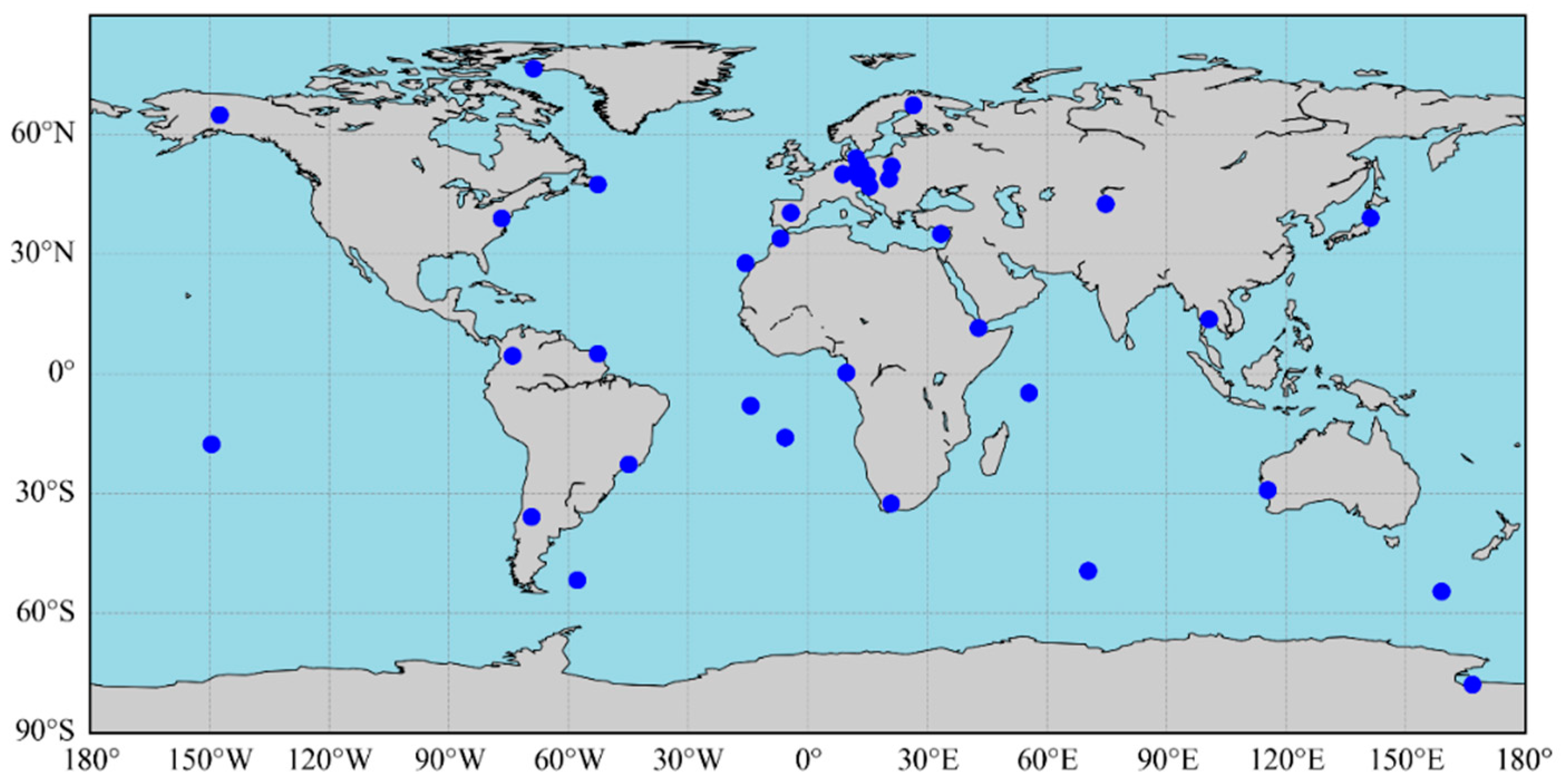
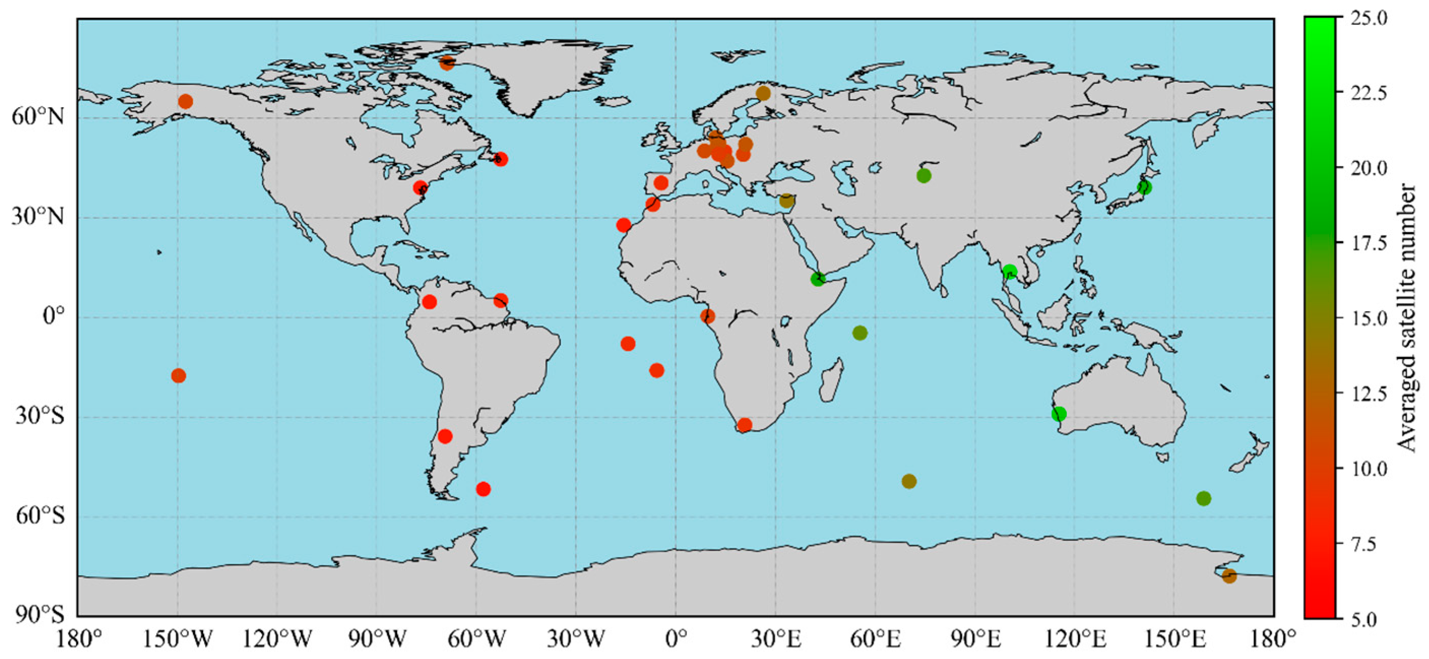
3. Data and Strategy

Figure 1 shows the 36 globally distributed MGEX stations for the PPP-AR tests. The stations are capable of tracking the GPS/Galileo/Glonass/BeiDou multi-GNSS, multi-frequency observations with the geodetic receiver. The experimental period was from day of year (DOY) 330 to 344 in 2023. To fully evaluate the performance of PPP-AR, the orbit, clock and phase-bias products with different time delay were utilized. These included post-stored CNES real-time products, GFZ rapid orbit/clock with phase biases estimated from CNES and the ambiguity-fixed clock/bias products from Wuhan University, labeled as “CNT”, “GBM”, and “WHU”, respectively. Additionally, various GNSS combinations were employed for the ambiguity-float and ambiguity-fixed PPP tests, including the single GPS (G), single BeiDou (C), GPS+Galileo (GE), GPS+BeiDou (GC) and the GPS+Galileo+BDS (GEC). The data are processed using both kinematic and static models. Convergence time is assessed using a positioning accuracy metric, indicating the duration until positioning errors in all East (E), North (N), and Up (U) components are below 10 cm for 10 consecutive epochs, respectively. After the convergence, positioning accuracy was evaluated by calculating the Root Mean Square (RMS) of the ENU components, with reference coordinates for each station derived from the IGS weekly solutions. Data leading to re-convergence during daily processing were excluded from the statistical analysis. Table 1 presents a detailed comparison of the signal types available in various products and those utilized for ionosphere-free (IF) PPP. Notably, rapid products encompass biases across all frequencies for all GNSS systems. However, a notable distinction exists in the biases for the real-time Galileo products: the “CNT” product includes Galileo biases on the Q channel, while the “GBM” product offers biases on the X channel. In contrast, the “WHU” products feature biases on both the X and Q channels.
All experiments were conducted using an in-house software developed on the G-Nut library platform [27]. The observations can be processed either in real-time mode or near real-time model, utilizing a forward Kalman filter or a backward smoothing method [28]. The code and phase biases are directly corrected in the raw observations during the pre-processing phase. Therefore, ambiguity-float PPP solutions are also computed with phase-bias-corrected observations if the phase biases are available in SINEX files. Both the ionosphere-free and raw models are supported with any arbitrary GNSS observation signal combinations by defining the GNSS observation types, frequencies, and channels in the configuration file. For achieving the ambiguity-fixed solution in the IF model, the MW combinations are used for the wide-lane ambiguity resolution, followed by narrow-lane ambiguity resolution using the LAMBDA method [29]. For the raw model, wide-lane ambiguity is initially resolved based on the raw float ambiguities of L1 and L2, and the fixed wide-lane ambiguity serves to constrain the float ambiguities in the raw PPP model. Subsequently, ambiguity resolution in the raw model is accomplished via the LAMBDA method. Additionally, the partial ambiguity resolution strategy is applied, wherein variance and ambiguity residuals are used to define subsets of ambiguities. The bias criteria are set at 0.25 and 0.15 cycles for wide-lane and narrow-lane ambiguities, respectively. The ratio test with a threshold of 2.0 is used for the narrow-lane ambiguity resolution. Detailed data-processing strategies are shown in Table 2.

4. Evaluation of PPP Using Geodetic Receivers

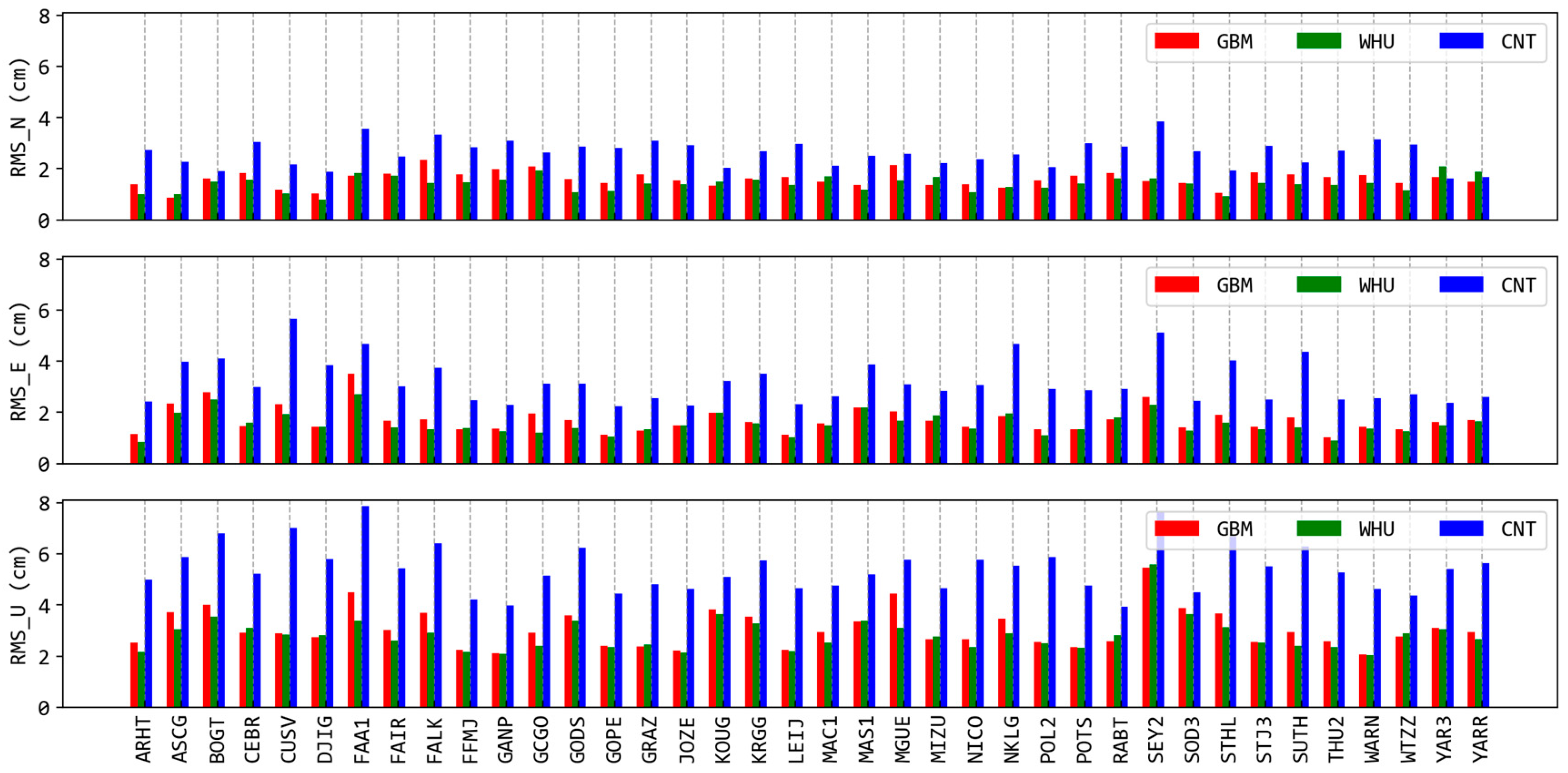
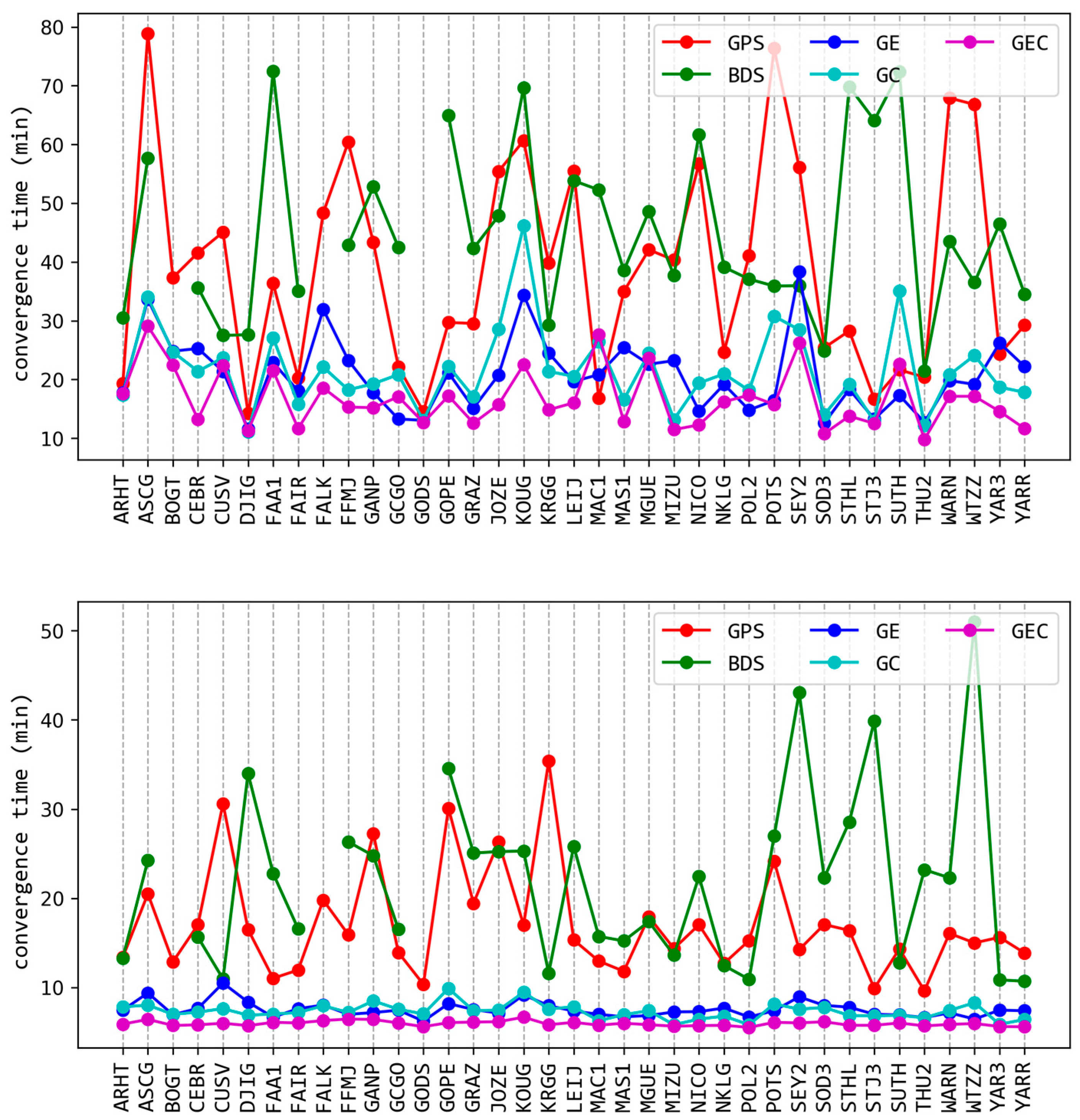
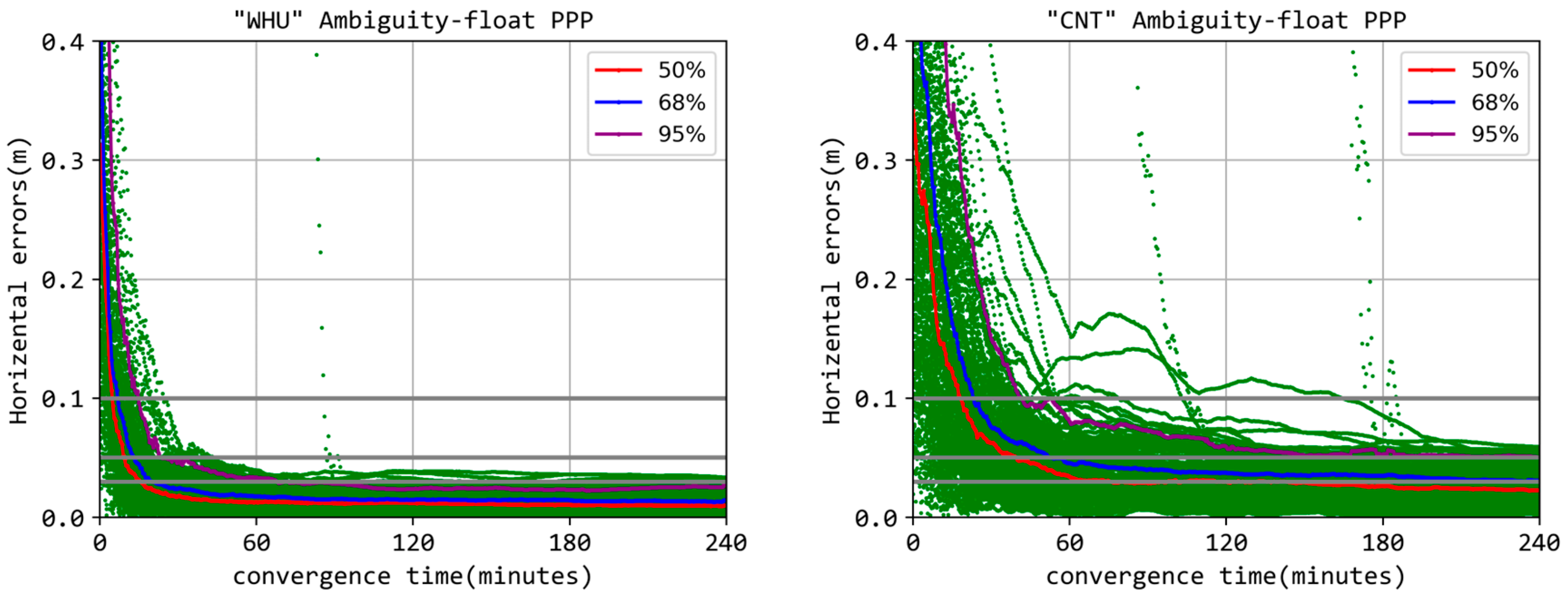
4.1. Multi-GNSS Kinematic Solution

In this section, we carry out kinematic PPP using 24 h of MGEX data, with both the ambiguity-float and ambiguity-fixed model. Figure 2 provides an overview of the averaged RMS values for each station after PPP convergence when using products from different agencies for GPS+Galileo ambiguity-fixed PPP. It can be observed that the RMS are relatively stable over different stations; however, there is a large difference in exits between the rapid products and real-time products. Furthermore, the accuracy from the “WHU” products is slightly better than that of the GBM products. The mean positioning accuracy of the kinematic PPP solutions for different stations are given in Table 3.
In the comparative analysis of PPP derived from different satellite system combinations, both the standalone GPS, GPS+Galileo- and GPS+Galileo+BDS-combined models exhibit comparable accuracy. These combinations consistently achieve horizontal accuracies within 2 cm and vertical accuracies within 4 cm in ambiguity-float PPP scenarios, employing rapid processing products (“GBM” and “WHU”). A marginal enhancement is observed in the GE-combined PPP relative to the standalone GPS approach, with only several improvements noted in the East and Up directions. This can be attributed to the inherent geometric robustness and precision of GPS products, which already offer substantial accuracy. On the contrary, incorporating BDS observations into PPP results in a reduction in positioning accuracy. This decrease could be attributed to the lower accuracy of BDS rapid products in multi-GNSS equal-weighting processing strategies. The single BDS PPP with “WHU” products and ambiguity-float PPP yield accuracies of only 3 cm, 3.9 cm, and 5.0 cm for the East, North, and Up components, respectively. Nevertheless, integrating GC observations markedly improves accuracy across these directions. Moreover, it is important to note that the positioning accuracy of the GEC combination is slightly inferior to that of GE and GC. This discrepancy arises because the accuracy is calculated from the time when the coordinate errors meet the convergence threshold of 0.1 m in each component until the end of processing. While multi-GNSS PPP can achieve faster convergence, resulting in more inaccurate coordinates included in the accuracy statistics, the overall accuracy is slightly diminished.
When evaluating PPP performance using various products, results achieved with rapid products outperform those obtained using real-time products (“CNT”), with “WHU” demonstrating superior accuracy across different products. The accuracy improvements of “WHU” products compared to “GBM” products range from 5% to 15%. These advancements are ascribed to the ambiguity-fixed clocks utilized by “WHU” products, enhancing overall performance. Moreover, accuracy enhancements range from 20% to 60% relative to “CNT” real-time products. The reduced accuracy associated with “CNT” products is linked to the inaccuracies of satellite orbit and clock products in real-time, especially concerning BDS. In the context of comparing positioning modes between ambiguity-float and ambiguity-fixed PPP, all phase-bias products facilitate an improvement in accuracy, except for BDS-only PPP. Notably, the horizontal accuracy improvements, particularly in the East component, surpass those in the vertical dimension. Overall, the GPS+Galileo-combined PPP, employing ambiguity fixing with “WHU” products, achieves the highest positioning accuracy, reaching 0.9 cm, 0.9 cm, and 2.6 cm for the North, East, and Up components, respectively. Real-time PPP using “CNT” products attains accuracies of 2.1 cm, 2.7 cm, and 4.8 cm for the North, East, and Up components, respectively, utilizing the GPS ambiguity-fixed PPP. The accuracy of BDS positioning is inferior to that of standalone GPS, with rapid products achieving accuracies of 3.0 cm, 3.9 cm, and 5.0 cm, and real-time products achieving 3.9 cm, 5.1 cm, and 6.7 cm, respectively. This discrepancy can be attributed to the inferior quality of BDS products, as well as the poor satellite geometry. To be specific, the global distribution of the stations and the average number of satellites are presented in Figure 3. Notably, only the stations located in the Asia–Pacific region have a better number of visible BDS satellites larger than 12, which is primarily attributed to the contribution of GEO and MEO satellites.
Figure 4 illustrates the variations in the average three-dimensional errors and satellite numbers for BDS-float PPP over all stations, sorted by the number of visible satellites. It is evident from the figure that there is a high correlation between positioning errors and the number of visible satellites. According to the statistics, when the number of visible satellites exceeds 10, the average positioning errors of BDS in the N, E, and U directions are 2.9 cm, 3.6 cm, and 5.5 cm, respectively.
Figure 5 illustrates the average convergence time required for ambiguity-float kinematic PPP employing various combinations of GNSS and rapid products from “WHU” at different stations. The analysis reveals that PPP with either GPS or BDS alone yields a comparable convergence duration of approximately 38.2 min to achieve 10 cm accuracy in three dimensions. However, this convergence time varies significantly across stations due to the satellite geometry. In terms of the multi-GNSS combinations, the integration of ‘GE’ and ‘GC’ effectively reduces the convergence time to 18.5 min. While the addition of BDS does not improve PPP accuracy, its significant contribution to reducing convergence time is clear. The combined use of three systems, namely, ‘GEC’, further shortens the average convergence time to 14.8 min. These observations highlight the advantage of multi-GNSS combinations in accelerating convergence times through improved satellite spatial geometry.
In ambiguity-float mode, where users lack an indicator to determine the convergence of PPP, understanding the duration to a specified accuracy can serve as a valuable metric for assessing PPP convergence. However, when employing the ambiguity resolution in PPP, the reliability of the solution is commonly gauged using the Time to First Fix (TTFF) metric. Hence, Figure 6 displays the average convergence times for ambiguity-fixed PPP, utilizing the TTFF metric. It reveals that the convergence times are 18.8 and 23.2 min for the standalone GPS and BDS PPP, respectively, marking a significant reduction of 51.5% and 38.4% compared to ambiguity-float PPP solutions. In the case of dual-GNSS combinations, a consistent average convergence time of 7.8 min is observed across different combinations. The combination of GPS, Galileo, and BDS further compresses the convergence time to 5 min. Note that gaps shown within the figure are attributed to the exclusion of data as outliers.
Statistics using the “GBM” rapid products are shown in Figure 7. The data show average convergence times of 38.3 min, 20.5 min and 16.7 min for the single-, dual- and triple-GNSS combinations with ambiguity-float PPP. After applying ambiguity fixing, the averaged TTFF is 18.6 min, 7.5 min and 6 min, respectively. Overall, the performance of PPP in terms of convergence time and accuracy after convergence from “WHU” products outperforms that of the “GBM” products. Consequently, the subsequent comparisons exclude the “GBM” products.
Additionally, solutions using the “CNT” real-time products, as illustrated in Figure 8 and Figure 9, reveal notably longer convergence times compared to those associated with “WHU” products. Specifically, the data show average convergence times of 50.4 min for standalone GPS, 42.6 min for dual-GNSS combinations, and 37.5 min for triple-GNSS combinations. This indicates that the convergence efficiency improvements facilitated by multi-GNSS observations are less marked with “CNT” products as opposed to “WHU” solutions. However, following the application of ambiguity resolution techniques, there is a substantial reduction in average convergence times to 22.6 min, 8.4 min, and 6.4 min, respectively. Note that the data gaps for GPS and BDS statistical results shown in Figure 8 indicate that the TTFF exceeds 2 h and, therefore, are excluded from the analysis.
Figure 10 illustrates the convergence of two-dimensional (2D) position errors for the “WHU” (top) and “CNT” (bottom) products with “GE” ambiguity-float (left) and ambiguity-fixed (right) solutions. The time series of the raw horizontal positioning errors are plotted with green points. Additionally, the corresponding 50%, 68%, and 95% quantiles are plotted in different colors, with positioning errors of 0.1 m highlighted in shades of grey. The results indicate that convergence times of 9.5, 15, and 36.5 min are necessary to reach the threshold at different probability levels using the “WHU” products and ambiguity-float PPP. These times can be shortened to 8, 10, and 32 min after the ambiguity resolution. For real-time processing, convergence times of 31, 42, and 108 min are required, and no improvement is observed with ambiguity resolution.
It is important to highlight that the convergence time measured by positioning accuracy differs from the results depicted in Figure 9, which utilize the TTFF metric.
Table 4 provides a summary of the convergence time for PPP utilizing various metrics. It is evident that the convergence time measured by the accuracy are reduced through ambiguity-fixing techniques; however, this is less apparent compared to the TTFF metric. This discrepancy arises because the accuracy enhancement resulting from ambiguity fixing typically operates at the centimeter to millimeter level. Figure 11 illustrates the positioning error series for station NICO using “GE” PPP on DOY 335, 2023, serving as an illustrative example. For the “WHU” and “CNT” products, the convergence time measured by the ambiguity-float PPP accuracy is 15.5 min, which decreases to 14.5 min after ambiguity fixing. However, it can be reduced to 7.5 min using the TTFF metric. Consequently, it is concluded that the TTFF achieved through ambiguity fixing should be perceived more as an indicator of a reliable PPP solution rather than a guarantee of high accuracy.

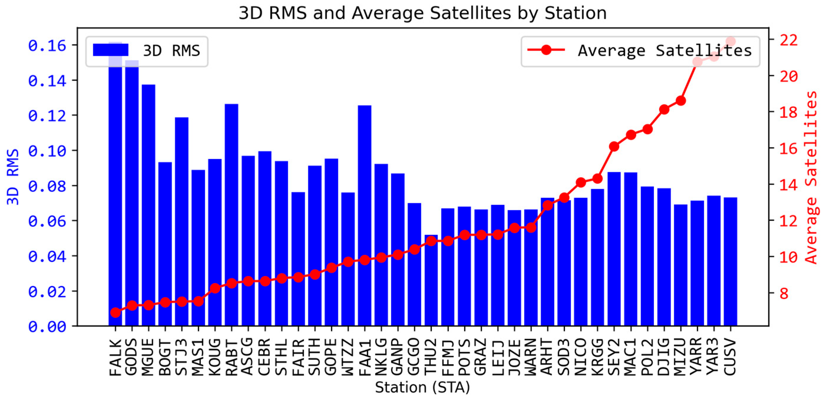
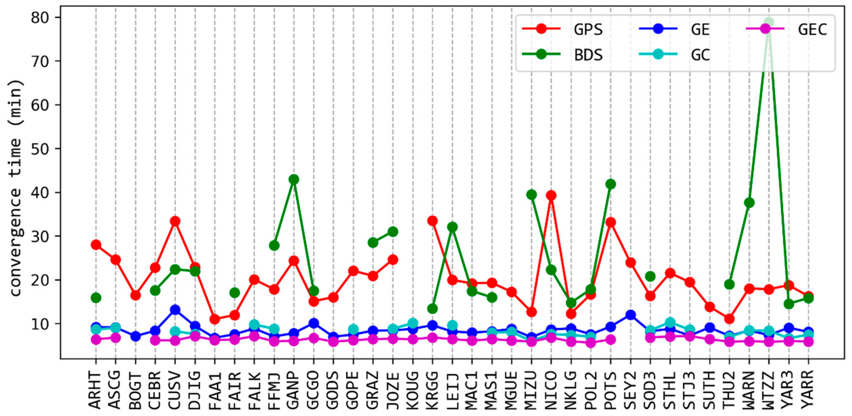
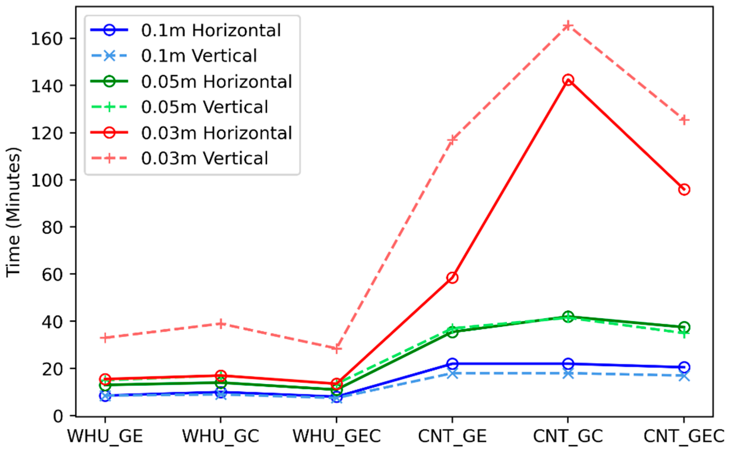
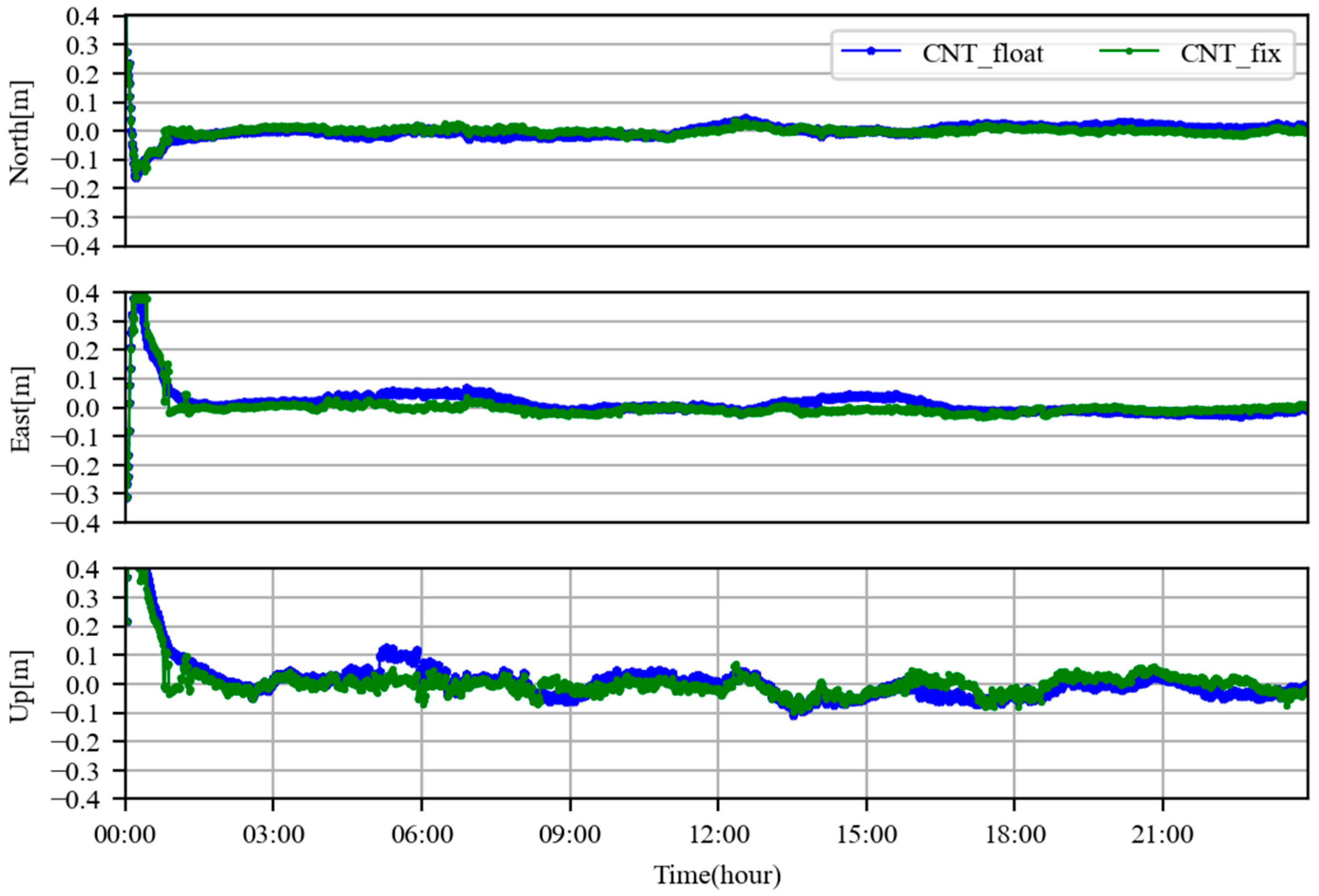
4.2. Multi-GNSS Static Solution

This section investigates the performance of multi-GNSS static PPP using various combinations. It has been demonstrated that the rapid products from “WHU” outperform the “GBM” products in terms of ambiguity-float and ambiguity-fixed PPP. In this analysis, “WHU” rapid products are utilized for rapid processing, alongside ‘CNT’ products for real-time PPP comparison. Targeting applications with rapid positioning is needed in the mass market; PPP sessions are performed with a duration of 4 h, amounting to 6 sessions for a single day’s processing. The convergence of horizontal and vertical positioning errors to thresholds of 0.1 m, 0.05 m, and 0.03 m serves as a statistical indicator to compare the performance of different solution combinations. Figure 12 presents the statistical results from the ambiguity-float PPP, calculated with different combinations, where 68% of positioning errors meet the specified thresholds. The results show that the convergence rate for the real-time ambiguity-float PPP with “CNT” products is slower compared to rapid products. On average, convergence to 0.1 m accuracy requires approximately 9.5 min for rapid products and 21.3 min for real-time products. For 0.05 m accuracy, the average convergence times are 19.1 min and 46.5 min, respectively. A notable difference in convergence times between rapid and real-time products becomes evident at the 0.03 m threshold, largely attributed to the lower accuracy of real-time products. This discrepancy requires extended observation periods to refine the filter’s estimated parameters. Statistical analysis reveals that achieving this accuracy level takes an average of 36.8 min with rapid products, compared to 221.7 min with real-time products. In comparison, Figure 13 illustrates convergence times for ambiguity-fixed PPP. Since the TTFF indicator has been shown to be insufficient for ensuring high accuracy in PPP, the convergence time of ambiguity-fixed PPP is also calculated using absolute positioning errors. Average convergence times of 8.8 min and 21.5 min are required for the rapid and real-time PPP errors to reach a 0.1 m threshold. For attaining a precision level of 0.05 m, the average required times are 12.6 min and 38.3 min, respectively, marking a 30.1% and 43.9% improvement over the float solution. A pronounced contrast is seen in the convergence to 0.03 m, especially in the vertical direction for real-time processing, which is significantly extended due to tropospheric decorrelation and the need for vertical coordinate convergence. The statistical findings confirm that an average duration of 33.5 min and 136 min are required for the vertical PPP to achieve 0.03 m accuracy using the rapid and real-time products. Figure 14 details the convergence of horizontal (left) and vertical (right) positioning errors for “GE”-combined PPP with “WHU” rapid products. The legend includes a red line for the 50% percentile, a blue line for the 68% percentile, and a purple line for the 98% percentile of errors. Three dashed grey lines indicate the accuracy convergence thresholds at 0.03 m, 0.05 m, and 0.1 m. It is clear that the vertical accuracy of PPP converges more slowly than its horizontal accuracy, and there are only minimal improvements in accuracy after 60 min. This slower convergence is primarily attributed to the inferior geometry of the vertical dilution of the position, which restricts the accuracy of PPP in the height direction.

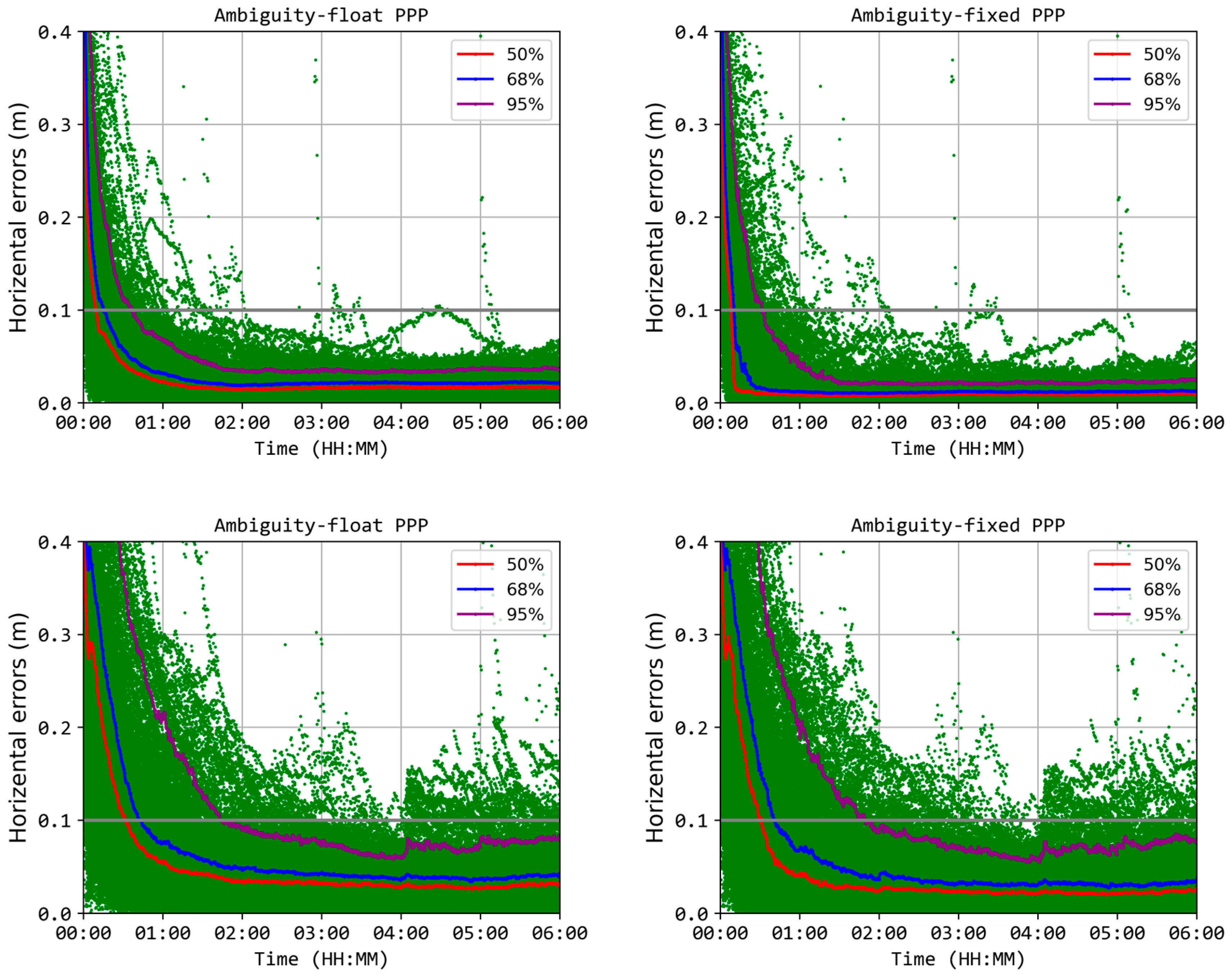
5. Evaluation of PPP Using Low-Cost Receivers

The analysis in the previous section was based on MGEX GNSS stations, which typically employ geodetic receivers. In contrast, this section focuses on static and kinematic PPP experiments conducted with low-cost GNSS receivers, which are more commonly used in mass market applications. The experiment took place from Day of Year (DOY) 300 to 315, 2023, at the Nanjing University of Information Science & Technology. A choke ring antenna, positioned in an open-sky environment and connected to a geodetic receiver for the Continuously Operating Reference Station service, was used. Two low-cost GNSS receivers, specifically the Septentrio Mosaic X5 and the Unicorecom UM980, were linked to the antenna via a signal splitter, establishing a zero-baseline configuration within the three GNSS receivers. The data are collected with a 5 s sampling rate, with PPP processing performed at a 30 s interval. Reference coordinates were determined by averaging the results from 30 days of static PPP using the geodetic receivers. The data collected from the two low-cost receivers were processed using the same strategies and combinations as those employed in the MGEX processing described in the previous section. Figure 15 presents the convergence time of the horizontal positioning errors for both ambiguity-float (top) and ambiguity-fixed (bottom) PPP, using the rapid products (left) and real-time products (right), with the GPS+Galileo+BDS-combined PPP.
The analysis revealed that 12 min and 50.5 min are required to achieve an accuracy of 0.05 m for the rapid and real-time products, respectively, with a 68% positioning error. By applying ambiguity resolution, the convergence times were reduced to 9.5 min and 47 min, respectively, resulting in improvements of 26.3% and 6.9%. The convergence time for the ambiguity-float PPP is even shorter than that of the MGEX stations. However, the results are overall consistent with those observed for MGEX stations, indicating that the accuracy of the products has a more significant impact on the accuracy of static PPP.
In kinematic PPP analysis, it is observed that a convergence time of 15 min is necessary to achieve an accuracy of 0.1 m using rapid products. The application of ambiguity fixing does not significantly reduce this convergence time. Conversely, when employing real-time products, the convergence time extends to 184 min and 157 min for ambiguity-float and ambiguity-fixed PPP, respectively. Notably, the convergence time for ambiguity-float PPP is considerably longer than that observed at MGEX stations in the previous section. For a detailed examination, Figure 16 and Figure 17 present a comparison of the convergence times for ambiguity-float and ambiguity-fixed PPP using rapid and real-time products, respectively. It is evident that the convergence time for real-time products is slower than that of the geodetic one. Upon the convergence of PPP, the accuracy of the “GE”-combined PPP in the North, East, and Up directions is found to be 1.8 cm, 3.1 cm, and 5.4 cm for the rapid products, and 1.1 cm, 1.8 cm, and 2.7 cm for the real-time products, respectively. The achieved accuracy after convergence is comparable to that observed at the MGEX stations.

6. Conclusions

PPP is becoming increasingly important in applications such as providing reference coordinates for relative positioning, rapid processing for aviation surveying data, and ocean sea level monitoring. Accuracy and convergence times are two critical indicators for PPP users, especially for the mass users using low-cost GNSS receivers. The emergence of phase biases for multi-GNSS and multi-frequency signals brings new opportunities for fast PPP(-AR). In this study, we evaluate the performance of PPP using real-time and rapid products with data from 36 globally distributed stations, as well data from two low-cost GNSS receivers. We assess the performance of ambiguity-float and ambiguity-fixed PPP in terms of static and kinematic modes using the rapid products from “WHU” and “GBM”, as well the real-time products from “CNT”.
In terms of the accuracy of kinematic PPP using different system combinations after convergence, the GPS+Galileo-combined PPP, employing ambiguity fixing with “WHU” products, achieves the highest positioning accuracy, reaching 0.9 cm, 0.9 cm, and 2.6 cm for the North, East, and Up components, respectively. Real-time PPP using “CNT” products attains accuracies of 2.1 cm, 2.7 cm, and 4.8 cm for the North, East, and Up components, respectively, utilizing the GPS ambiguity-fixed PPP. The accuracy of BDS positioning is inferior to that of standalone GPS, with rapid products achieving accuracies of 3.0 cm, 3.9 cm, and 5.0 cm, and real-time products achieving 3.9 cm, 5.1 cm, and 6.7 cm, respectively. When the number of visible BDS satellites exceeds 10, the average positioning errors can be improved to 2.9 cm, 3.6 cm, and 5.5 cm, respectively.
Then, a convergence time to achieve 10 cm accuracy and the TTFF indicator are used to evaluate the convergence time of kinematic ambiguity-float and ambiguity-fixed PPP. Approximately 38.2 min is required for the single GNSS; the time can be shortened to 18.5 min for dual-system combinations. Additionally, the time can be further shortened to 14.8 min for the triple-system combinations. For the ambiguity-fixed PPP, the TTFF metrics are reduced by 51.5% and 38.4% for single GPS and BDS PPP to 18.8 cm and 23.2cm. The convergence time can be further shortened to 7.8 min using the multi-GNSS combinations. In terms of the real-time products, 37.5 min and 8.4 min are required for the ambiguity-float and ambiguity-fixed PPP. However, the TTFF should be seen more as an indicator of reliable PPP convergence rather than convergence to high accuracy.
In the context of static PPP using various GNSS combinations and precise products, it has been observed that the choice of GNSS combination does not significantly influence the convergence times; instead, these times are more dependent on the precision of the products employed. Specifically, real-time products take approximately 22 min to achieve horizontal accuracy below 0.1 m, while rapid products reach this accuracy within 10 min. However, applying ambiguity fixing does not bring notable improvements. For the accuracy threshold of 0.05 m, convergence times of 19.1 min and 46.5 min are required for rapid and real-time products, respectively. In this case, ambiguity fixing can reduce the convergence times to 13 min and 39 min, respectively. If aiming for an even higher precision of 0.03 m, the required convergence times would need to be extended to 36.8 min for rapid products, and real-time products would require more than two hours.
For PPP using low-cost GNSS receivers, more than two hours is necessary to achieve an accuracy better than 0.1 m for both the ambiguity-float and ambiguity-fixed kinematic PPP, which is considerably longer than the convergence time observed at MGEX stations. However, the accuracy achieved after convergence is comparable to that observed at MGEX stations. Additionally, static PPP requires 12 min and 50.5 min to achieve an accuracy of 0.05 m for the rapid and real-time products, respectively, and the convergence time can be reduced to 9.5 min and 47 min after ambiguity resolution. The performance is also comparable to that of the MGEX stations.

Author Contributions

Conceptualization, L.Z., Y.L. and S.J.; methodology, L.Z. and Y.L.; validation, M.C. and W.Z.; formal analysis, M.C. and W.Z.; writing—original draft preparation, M.C. and W.Z.; writing—review and editing, S.J., L.Z. and Y.L. All authors have read and agreed to the published version of the manuscript.

Funding

This research was funded by the National Natural Science Foundation of China (42104018, 42204029), China Postdoctoral Science Foundation (2022M711669).

Data Availability Statement

The GNSS observations used in this study can be accessed at https://cddis.nasa.gov/archive (accessed on 17 April 2024). Wuhan University provides GPS/Galileo/BDS phase clock/bias products at ftp://igs.gnsswhu.cn/pub/whu/phasebias/ (accessed on 17 April 2024). CNES provides GPS/Galileo/BDS products corresponding to GFZ orbit/clock products at http://www.ppp-wizard.net/products/POST_PROCESSED/ (accessed on 17 April 2024), and real-time products at http://www.ppp-wizard.net/products/REAL_TIME/ (accessed on 17 April 2024).

Acknowledgments

The authors gratefully acknowledge IGS MGEX for providing the GNSS data. We also acknowledge the CNES and Wuhan University for providing real-time and rapid precise products.

Conflicts of Interest

The authors declare no conflicts of interest.

References

  1. Zumberge, J.F.; Heflin, M.B.; Jefferson, D.C.; Watkins, M.M.; Webb, F.H. Precise Point Positioning for the Efficient and Robust Analysis of GPS Data from Large Networks. J. Geophys. Res. Soild Earth 1997, 102, 5005–5017. [Google Scholar] [CrossRef]
  2. Jin, S.; Su, K. PPP models and performances from single-to quad-frequency BDS observations. Satell. Navig. 2020, 1, 16. [Google Scholar] [CrossRef]
  3. Zhang, B.; Hou, P.; Zha, J.; Liu, T. PPP–RTK functional models formulated with undifferenced and uncombined GNSS observations. Satell. Navig. 2022, 3, 3. [Google Scholar] [CrossRef]
  4. Zheng, K.; Liu, K.; Zhang, X.; Wen, G.; Chen, M.; Zeng, X.; Zhao, L.; He, X. First results using high-rate BDS-3 observations: Retrospective real-time analysis of 2021 Mw 7.4 Madoi (Tibet) earthquake. J. Geod. 2022, 96, 51. [Google Scholar] [CrossRef]
  5. Zheng, K.; Zhang, X.; Li, X.; Li, P.; Sang, J.; Ma, T.; Schuh, H. Capturing coseismic displacement in real time with mixed single- and dual-frequency receivers: Application to the 2018 Mw7.9 Alaska earthquake. GPS Solut. 2019, 23, 9. [Google Scholar] [CrossRef]
  6. Ge, M.; Gendt, G.; Rothacher, M.; Shi, C.; Liu, J. Resolution of GPS carrier-phase ambiguities in Precise Point Positioning (PPP) with daily observations. J. Geod. 2008, 82, 389–399. [Google Scholar] [CrossRef]
  7. Laurichesse, D.; Mercier, F.; Berthias, J.-P.; Broca, P.; Cerri, L. Integer Ambiguity Resolution on Undifferenced GPS Phase Measurements and Its Application to PPP and Satellite Precise Orbit Determination. Navigation 2009, 56, 135–149. [Google Scholar] [CrossRef]
  8. Melbourne, W.G. The case for ranging in GPS-based geodetic systems. In Proceedings of the First International Symposium on Precise Positioning with the Global Positioning System, Rockville, MD, USA, 15–19 April 1985; pp. 373–386. [Google Scholar]
  9. Wübbena, G. Software developments for geodetic positioning with GPS using TI-4100 code and carrier measurements. In Proceedings of the First International Symposium on Precise Positioning with the Global Positioning System, Rockville, MD, USA, 15–19 April 1985; Volume 19, pp. 403–412. [Google Scholar]
  10. Collins, P.; Lahaye, F.; Héroux, P.; Bisnath, S. Precise Point Positioning with Ambiguity Resolution using the Decoupled Clock Model. In Proceedings of the 21st International Technical Meeting of the Satellite Division of the Institute of Navigation (ION GNSS 2008), Savannah, GA, USA, 16–19 September 2008; pp. 1315–1322. [Google Scholar]
  11. Geng, J.; Chen, X.; Pan, Y.; Zhao, Q. A modified phase clock/bias model to improve PPP ambiguity resolution at Wuhan University. J. Geod. 2019, 93, 2053–2067. [Google Scholar] [CrossRef]
  12. Gazzino, C.; Blot, A.; Bernadotte, E.; Jayle, T.; Laymand, M.; Lelarge, N.; Lacabanne, A.; Laurichesse, D. The CNES Solutions for Improving the Positioning Accuracy with Post-Processed Phase Biases, a Snapshot Mode, and High-Frequency Doppler Measurements Embedded in Recent Advances of the PPP-WIZARD Demonstrator. Remote Sens. 2023, 15, 4231. [Google Scholar] [CrossRef]
  13. Geng, J.; Wen, Q.; Zhang, Q.; Li, G.; Zhang, K. GNSS observable-specific phase biases for all-frequency PPP ambiguity resolution. J. Geod. 2022, 96, 11. [Google Scholar] [CrossRef]
  14. Su, K.; Jin, S.; Hoque, M.M. Evaluation of ionospheric delay effects on multi-GNSS positioning performance. Remote Sens. 2019, 11, 171. [Google Scholar] [CrossRef]
  15. Zhang, B.; Zhao, C.; Odolinski, R.; Liu, T. Functional model modification of precise point positioning considering the time-varying code biases of a receiver. Satell. Navig. 2021, 2, 11. [Google Scholar] [CrossRef]
  16. Shu, B.; Tian, Y.; Qu, X.; Li, P.; Wang, L.; Huang, G.; Du, Y.; Zhang, Q. Estimation of BDS-2/3 phase observable-specific signal bias aided by double-differenced model: An exploration of fast BDS-2/3 real-time PPP. GPS Solut. 2024, 28, 88. [Google Scholar] [CrossRef]
  17. Zheng, K.; Tan, L.; Liu, K.; Li, P.; Chen, M.; Zeng, X. Multipath mitigation for improving GPS narrow-lane uncalibrated phase delay estimation and speeding up PPP ambiguity resolution. Measurement 2023, 206, 112243. [Google Scholar] [CrossRef]
  18. Schaer, S. Bias-SINEX Format and Implications for IGS Bias Products; IGS Workshop: Sydney, Australia, 2016; pp. 8–12. [Google Scholar]
  19. Cao, X.; Yu, X.; Ge, Y.; Liu, T.; Shen, F. BDS-3/GNSS multi-frequency precise point positioning ambiguity resolution using observable-specific signal bias. Measurement 2022, 195, 111134. [Google Scholar] [CrossRef]
  20. Geng, J.; Yang, S.; Guo, J. Assessing IGS GPS/Galileo/BDS-2/BDS-3 phase bias products with PRIDE PPP-AR. Satell. Navig. 2021, 2, 17. [Google Scholar] [CrossRef]
  21. Du, S.; Shu, B.; Xie, W.; Huang, G.; Ge, Y.; Li, P. Evaluation of Real-time Precise Point Positioning with Ambiguity Resolution Based on Multi-GNSS OSB Products from CNES. Remote Sens. 2022, 14, 4970. [Google Scholar] [CrossRef]
  22. Li, B.; Ge, H.; Bu, Y.; Zheng, Y.; Yuan, L. Comprehensive assessment of real-time precise products from IGS analysis centers. Satell. Navig. 2022, 3, 12. [Google Scholar] [CrossRef]
  23. Gill, M.; Bisnath, S.; Aggrey, J.; Seepersad, G. Precise Point Positioning (PPP) using Low-Cost and Ultra-Low-Cost GNSS Receivers. In Proceedings of the 30th International Technical Meeting of the Satellite Division of The Institute of Navigation (ION GNSS+ 2017), Portland, OR, USA, 25–29 September 2017; pp. 226–236. [Google Scholar]
  24. Romero-Andrade, R.; Trejo-Soto, M.E.; Vega-Ayala, A.; Hernández-Andrade, D.; Vázquez-Ontiveros, J.R.; Sharma, G. Positioning Evaluation of Single and Dual-Frequency Low-Cost GNSS Receivers Signals Using PPP and Static Relative Methods in Urban Areas. Appl. Sci. 2021, 11, 10642. [Google Scholar] [CrossRef]
  25. Ogutcu, S.; Alcay, S.; Duman, H.; Ozdemir, B.N.; Konukseven, C. Static and kinematic PPP-AR performance of low-cost GNSS receiver in monitoring displacements. Adv. Space Res. 2023, 72, 4795–4808. [Google Scholar] [CrossRef]
  26. Wang, L.; Li, Z.; Wang, N.; Wang, Z. Real-time GNSS precise point positioning for low-cost smart devices. GPS Solut. 2021, 25, 69. [Google Scholar] [CrossRef]
  27. Vaclavovic, P.; Dousa, J.; Gyori, G. G-Nut software library—State of development and first results. Acta Geodyn. Geomater. 2013, 10, 431–436. [Google Scholar] [CrossRef]
  28. Vaclavovic, P.; Dousa, J. Backward smoothing for precise GNSS applications. Adv. Space Res. 2015, 56, 1627–1634. [Google Scholar] [CrossRef]
  29. Teunnissen, P.J.G. The least-square ambiguity decorrelation adjustment: A method for fast GPS integer ambiguity estimation. J. Geod. 1995, 70, 65–82. [Google Scholar] [CrossRef]
  30. Saastamoinen, J. Contributions to the Theory of Atmospheric Refraction. J. Geod. 1972, 105, 279–298. [Google Scholar] [CrossRef]
  31. Boehm, J.; Niell, A.E.; Tregoning, P.; Schuh, H. Global mapping function (GMF): A new empirical mapping function based on numerical weather model data. Geophys. Res. Lett. 2006, 25, L07304. [Google Scholar] [CrossRef]
  32. Petit, G.; Luzum, B. IERS Conventions; IERS Tech. Note 36; Verlag des Bundesamts für Kartographie und Geodäsie: Frankfurt am Main, Germany, 2010. [Google Scholar]
Figure 1. Distribution of stations used for the PPP experiments.
Remotesensing 16 01434 g001
Figure 2. RMS values for station-specific GPS+Galileo ambiguity-fixed kinematic PPP.
Remotesensing 16 01434 g002
Figure 3. The distribution of stations with the number of available BDS satellites.
Remotesensing 16 01434 g003
Figure 4. Average 3D RMS for each station as well as the number of visible satellites.
Remotesensing 16 01434 g004
Figure 5. Average float convergence time for each station using different system combinations with “WHU” products.
Remotesensing 16 01434 g005
Figure 6. The convergence time of ambiguity-fixed PPP using the TTFF metric for each station using different GNSS combinations with “WHU” products.
Remotesensing 16 01434 g006
Figure 7. Average float (top) and fixed (bottom) convergence time for each station using different system combinations with “GBM” products.
Remotesensing 16 01434 g007
Figure 8. Average float convergence time for each station using different system combinations with “CNT” products.
Remotesensing 16 01434 g008
Figure 9. Average TTFF for each station using different system combinations with “CNT” products.
Remotesensing 16 01434 g009
Figure 10. The horizontal positioning errors (green) alongside their 50% (red), 68% (blue), 95% (purple) quantiles from “GE” PPP with “WHU” (top) and “CNT” (bottom) products.
Remotesensing 16 01434 g010
Figure 11. Time series of positioning errors for station NICO on DOY 335, 2023, using “GE”-combined PPP with “WHU” (left) and “CNT” (right) products.
Remotesensing 16 01434 g011
Figure 12. The convergence time of the horizontal and vertical positioning errors for ambiguity-float PPP to different thresholds by different processing combinations.
Remotesensing 16 01434 g012
Figure 13. The convergence time of the horizontal and vertical positioning errors for ambiguity-fixed PPP to different thresholds by different processing combinations.
Remotesensing 16 01434 g013
Figure 14. The positioning errors (green) alongside their 50% (red), 68% (blue), 95% (purple) quantiles for the horizontal (left) and vertical (right) components from ambiguity-fixed “GE” PPP with “WHU” products.
Remotesensing 16 01434 g014
Figure 15. The positioning errors (green) alongside their 50% (red), 68% (blue), 95% (purple) quantiles for ambiguity-float (top) and ambiguity-fixed (bottom) “GEC”-combined PPP using the “WHU” and “CNT” products.
Remotesensing 16 01434 g015aRemotesensing 16 01434 g015b
Figure 16. The positioning error series for the kinematic PPP using the ambiguity-float and ambiguity-fixed solution with real-time products.
Remotesensing 16 01434 g016
Figure 17. Positioning error series for the kinematic PPP using the ambiguity-float and ambiguity-fixed solution with rapid products.
Remotesensing 16 01434 g017
Table 1. Details of biases available in products and the used biases.
LabelsTypeSystemsSignals Used for PPP
CNTReal-timeGPS
Galileo
Glonass
BDS-2/BDS-3
GPS:C1C/C2W/L1C/L2W
Galileo:C1C/C5Q/L1C/L5Q
BDS:C2I/C6I/L2I/L6I
WHURapidGPS:C1W/C2W/L1C/L2W
Galileo:C1C/C5Q/L1C/L5Q
C1X/C5X/L1X/L5X
BDS:C2I/C6I/L2I/L6I
GBMRapidGPS:C1W/C2W/L1C/L2W
Galileo:C1X/C5X/L1X/L5X
BDS:C2I/C6I/L2I/L6I
Table 2. Data-processing strategies of PPP-AR.
ParameterConfigurations
Observations FrequencyGPS:L1/L2 Galileo:E1/E5a
BDS-2/BDS-3:B2I/B6I
EstimatorExtended Kalman filter
observation noisePseudorange: 0.3 m; carrier-phase: 0.003 m
Cutoff elevation
Ionosphere delaysionosphere-free combination
Troposphere delaysSaastamoinen [30] + Global Mapping Function [31]
Weighting strategyElevation-dependent weighting
Antenna phase centersIgs20.atx
Tidal displacementsCorrected [32]
Relativistic effectCorrected
Satellite attitudeNominal
Receiver clocksOne for each GNSS as a white-noise-like parameter; ISB estimated for the BDS-2 and BDS-3 with the BDS-2 down weighting
Table 3. Statistical results for the kinematic position accuracy of the ambiguity-float and ambiguity-fixed solutions.
SystemProductFloatFixedFloat to Fixed Improvements
NEUNEUNEU
GPSGBM1.41.93.41.11.32.921%32%15%
WHU1.31.8311.22.623%33%13%
CNT2.33.15.12.12.74.89%13%6%
BDSGBM3.04.05.72.93.963%3%−5%
WHU3.03.952.83.75.47%5%−8%
CNT3.95.16.745.36.9−3%−4%−3%
GPS+BDSGBM1.723.51.31.43.324%30%6%
WHU1.51.731.11.12.927%35%3%
CNT3.44.56.93.44.46.90%2%0%
GPS+GALGBM1.61.731.112.931%41%3%
WHU1.41.52.80.90.92.636%40%7%
CNT2.63.25.42.42.75.28%16%4%
GPS+GAL+BDSGBM1.71.93.11.31.2324%37%3%
WHU1.51.62.81.112.727%38%4%
CNT33.65.72.83.35.67%8%2%
Table 4. Statistical analysis on the convergence time of PPP using different GNSS combinations and convergence metrics.
Ambiguity-Float PPP with 10 cm Accuracy MetricAmbiguity-Fixed PPP with 10 cm Accuracy MetricAmbiguity-Fixed PPP with TTFF Metric
Single-GNSSDual-GNSSTriple-GNSSSingle-GNSSDual-GNSSTriple-GNSSSingle-GNSSDual-GNSSTriple-GNSS
WHU38.218.514.833.315.713.1217.85
GBM38.320.516.731.917.115.618.67.56
CNT50.442.637.548.343.136.522.68.46.4
Disclaimer/Publisher’s Note: The statements, opinions and data contained in all publications are solely those of the individual author(s) and contributor(s) and not of MDPI and/or the editor(s). MDPI and/or the editor(s) disclaim responsibility for any injury to people or property resulting from any ideas, methods, instructions or products referred to in the content.

