Application of Polynomial Interpolation for Iterative Complementation of the Missing Nodes in a Regular Network of Squares Used for the Construction of a Digital Terrain Model

Abstract

Due to the continuous increase in the volume of spatially located information, the current requirements imposed on the Spatial Information System (SIS) concern increasing data mining capabilities. Modern measurement systems, based on devices which enable the automatic recording of observation results on a mass scale (LiDAR—Light Detection and Ranging, MBES—Multi Beam Echo Sounder, etc.), allow for a very large volume of information on the surface to be measured and acquired in a relatively short time. One of the methods to reduce the volume of data enabling the generation of a model surface is to convert unevenly distributed measurement points into a regular network of squares (GRID). However, the generation of a complete grid is not always possible. In the measurement spectrum, there may be areas where measurement points have not been recorded. Measurement points can also be eliminated by either filtering the erroneously recorded data or eliminating the measured vegetation or the utilities in the area. To address these problems, the current article proposes a method for complementing the missing internal nodes in a regular network of squares using polynomial interpolation algorithms. Moreover, the paper demonstrates the possibilities of using the presented method for adding additional points between the already existing nodes of the network of squares. The application of the methodology presented in this article enables the effective elimination of (or a reduction in) the gaps in the GRID structure, which, in turn, allows such a network of squares to be used to generate a more accurate Digital Terrain Model.

1. Introduction

Thanks to the development of measurement techniques, opportunities are currently arising to record an increasing amount of new, previously unmeasurable information about the surrounding world [1,2,3]. At the same time, both the resolution and measurement accuracy of all objects that have been subject to measurement are increasing [4,5]. Furthermore, much of the information stored in modern Spatial Information Systems (SISs) is subject to dynamic changes over a relatively short period. The dynamics of the changes taking place in the surrounding space additionally imply the multiple recording of phenomena in the same area in different measurement epochs [6,7,8]. The collection and processing of such data impose particularly demanding requirements on the Spatial Information System, especially when supporting increased database resources [9,10,11]. In pursuit of this task, not only the methods for collecting and sharing information but also (and above all) the data processing optimisation techniques must evolve. Particular emphasis is placed on reducing the volume of data and keeping the resources up-to-date in real time [12,13,14]. At the same time, the use of new data acquisition technologies (LiDAR—Light Detection and Ranging; MBES—Multi Beam Echo Sounder; InSAR—Interferometric Synthetic Aperture Radar, etc.), in which the selection of the measured points and their recording take place without human intervention, necessitates the search for new methods for processing measurement results [15,16,17,18]. All of this results in an exponential increase in the volume of information requiring ongoing processing and analysis [19,20].

One of the basic tasks that are undertaken in the complex process of constructing the Spatial Information System is the development of a Digital Terrain Model (DTM) [21,22]. DTM is one of the basic information layers used by systems that describe phenomena in terms of value and often provides them with the basis of spatial organisation [23,24]. As the environment is being transformed, DTM is also subject to continuous changes and should, therefore, be updated on an ongoing basis. The specificity and the universal nature of the information layer, which comprises data on the relief or land surface coverage, lead one to place a particular emphasis on organising the recording of the data making up the model, minimising their number, and eliminating redundancy as much as possible [25,26]. In order to achieve high dynamics in the creation and administration of the generated DTMs, the aim is to ensure the maximum efficiency of the processing process, for which the final product is a surface model generated on the basis of the minimum amount of data while maintaining its maximum accuracy [27,28].

When striving to develop a Digital Terrain Model, a number of factors that determine the accuracy and quality of the development of this model in the SIS need to be taken into account [29,30]. The DTM representation in the Spatial Information System is usually created on the basis of the structures of the Triangulated Irregular Network (TIN) or the Regular Network of Squares (GRID) [31,32,33]. In order to organise the information describing the space using x, y, and h coordinates (e.g., terrain, seabed, or surface engineering features) and to reduce redundancy in the database resources, the numerical surface is presented as a regular grid of nodes that form a GRID-type structure [34,35]. Most modern Spatial Information Systems enable the creation and visualisation of a digital terrain model based on the regular grid uniformly covering the measurement area [36,37]. Such grids can be constructed on different regular base shapes (squares, equilateral triangles, regular hexagons) but, most often, when generating DTM in the Spatial Information System, the Regular Network of Squares is used, for which the points that make up the model are distributed at the corners of squares with a specific side length [38,39].

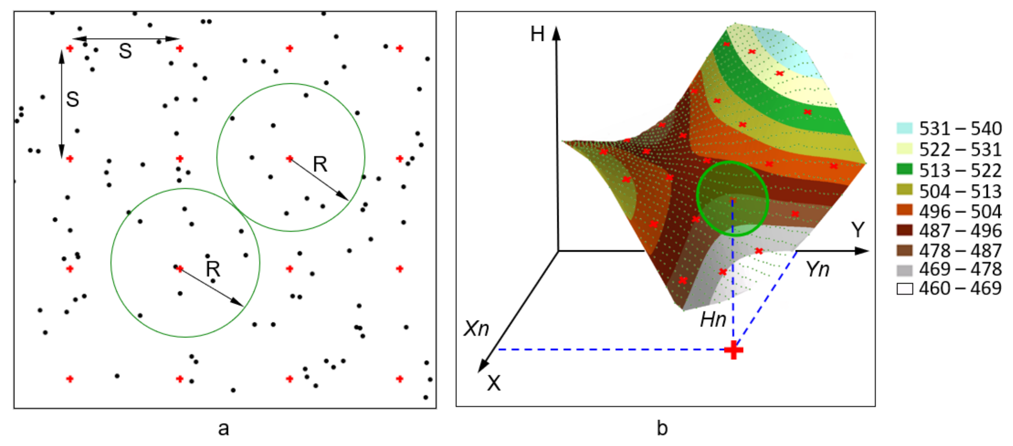
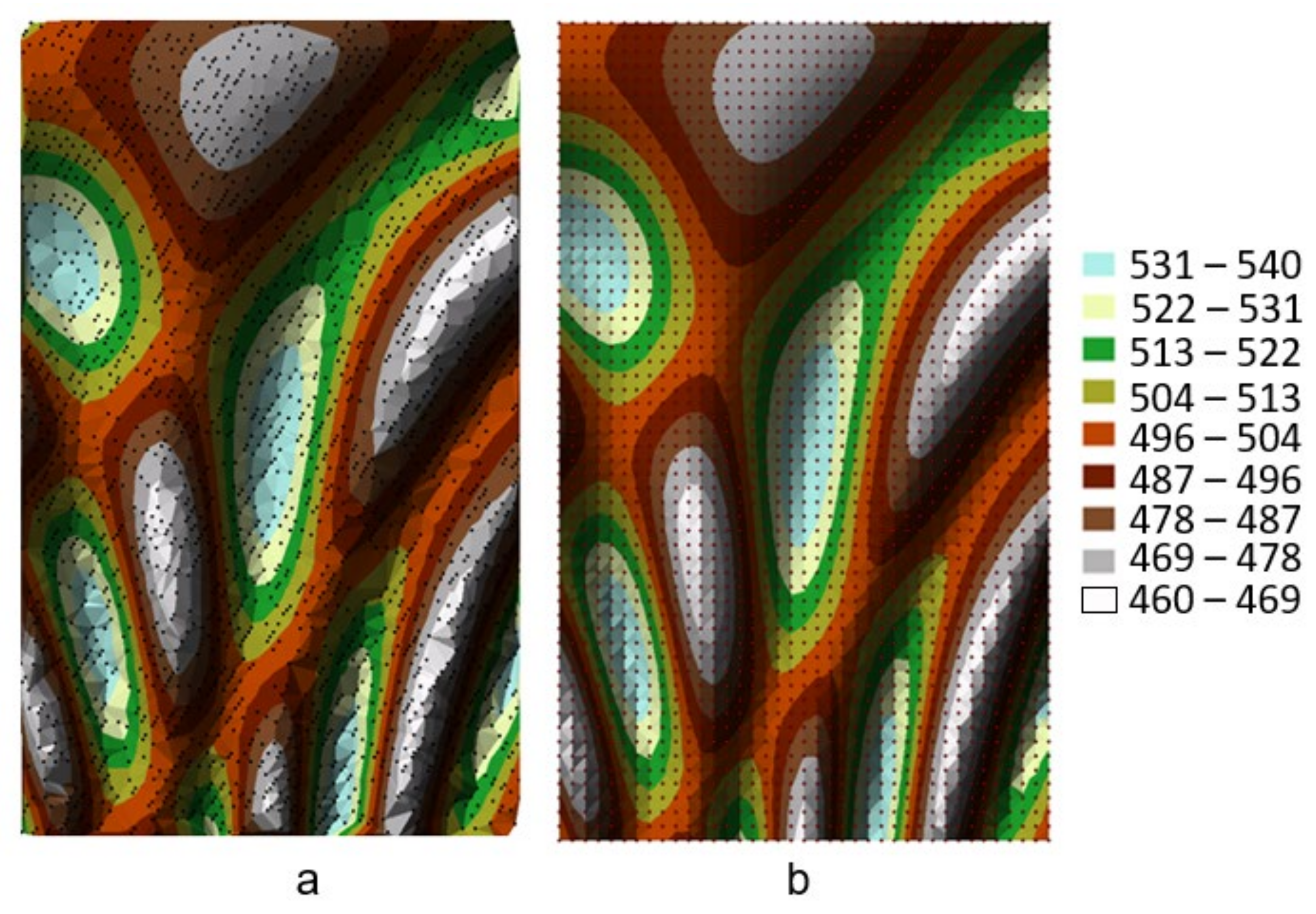
As regards the GRID structure, the position of the square corners (nodes) on the XY plane (on a specific part of the surface) is determined by the fixed distance interval (S = constant) in both directions of the axis (Figure 1a). The measurement points involved in determining a value at a node are found within a fixed search radius R (Figure 1a). The spacing S between individual nodes determines the resolution of the grid and, ultimately, the number of points generating the GRID model in a particular area [40,41,42].

Each node of the GRID structure is assigned a mathematically defined pair of coordinates (Xn and Yn), while the third coordinate Hn is determined by interpolation based on measurement points found in the assumed search radius (Figure 1b). Numerous different interpolation methods are described in the literature [43,44,45]. They enable the determination of the surface using a set of nodes whose coordinates were calculated on the basis of measurement data. The determination of the relevant construction parameters of the GRID structure enables the determination of the location of the interpolated point grid and its resolution, which is determined by a number of factors. This is most often determined by the availability and density of measurement points, the morphology of the surface being measured, the type of interpolation algorithm used, or the accuracy of the final compilation [46,47]. The entire process of node determination, which is also referred to as gridding, can be defined as the interpolation of the Hw value at the nodes of a regular grid (with the coordinates of Xw, Yw) based on the function value at measurement points (with the coordinates x, y, h) [48,49,50].

When creating a surface model using the GRID structure, the aim should be to obtain as complete a grid of nodes as possible over the study area. A complete structure contributes to increasing the accuracy of surface modelling and improving the quality of spatial analysis [51,52]. A complete grid structure for each measurement epoch is also required during the analyses of changes in the surface model over time. An adequate density of such a structure allows analyses of changes in DTM in successive measurement epochs to be carried out at any point of the space under analysis [53,54].

However, due to the specificity of data processing during the gridding process, the GRID structure generated on the basis of the nodes is not always complete. The diverse spatial distribution of measurement points does not always ensure the uniform coverage of the surface being measured. In the measurement spectrum, there may be areas of varying measurement point density and unintentional data gaps, causing shortages and voids in the resource being acquired [55,56]. Moreover, due to the need to identify the points located on the topographic surface, a proportion of the measurement information is filtered out. The completion of this processing step also leaves the data, which do not always cover the measured object in its entirety in the measurement spectrum. As regards LiDAR measurements, the measurement points reflected from the utilities or the vegetation cover are rejected [57,58,59]. The filtering process eliminates the measurement points recorded with errors or excludes the reflections of the measurement beam from the objects not being measured in a particular project. For this reason, a portion of measurement data is thinned out, which results in additional variation in the density of measurement points and additional gaps in the continuity of measurement coverage of the entire surface [60,61]. The determination of a complete grid of nodes is also not always possible due to the requirements of a particular interpolation method. For the accurate determination of the nodes, different interpolation methods require a specific location of measurement points, which, when their density is low, is not always possible to ensure [62,63]. The zones of the potential occurrence of nodes can be identified by using the areas of occurrence of measurement points in a selected spatial configuration [64,65]. In this situation, the shortages and voids in the measurement spectrum coincide with the gaps in the node structure being generated. The nodes that are subject to elimination are those which do not have a suitable location for measurement points for a particular interpolation method or are impossible to determine due to an insufficient (in relation to the assumed or the required) number of measurement points located in a defined search space [66,67]. In addition, the performed check of the interpolation model accuracy eliminates, from the resulting resource, the nodes that do not satisfy the adopted accuracy assumptions or cause too much local disturbance of the surface model (e.g., places of discontinuity of the model, determined by extrapolation) [68,69]. Due to all the above-mentioned factors, an incomplete GRID structure can be found in the resulting datasets, which contributes to the reduced quality of the final interpolation model and hinders the performance of comprehensive spatial analyses. The presented methodology focused on the solutions that enable the elimination (or reduction) of undesirable shortages of nodal points in the generated GRID structure.

2. Materials and Methods

The proposed methodology applied the single-pass and iterative method for complementing the missing nodes. In both cases, the existing (incomplete) nodes do not change their location in space. Based on these, nodes complementing the GRID structure are generated in a manner that ensures a grid that is as complete as possible is obtained. Furthermore, both methods of complementing the GRID structure can also be used to increase the resolution of the analysed grid of nodes. In the methodology presented, data are successfully transferred between the execution modules in a direct manner (by using the same address space of indexed variables, which accelerates the processing process) or using files (binary or text) which enable the generation of intermediate results and subjecting them to accuracy checks. Thus, after an initial assessment of the quality of the models generated, the parameters of processing the next iteration can be defined and used to improve the quality of the model and the checks on the entire process.

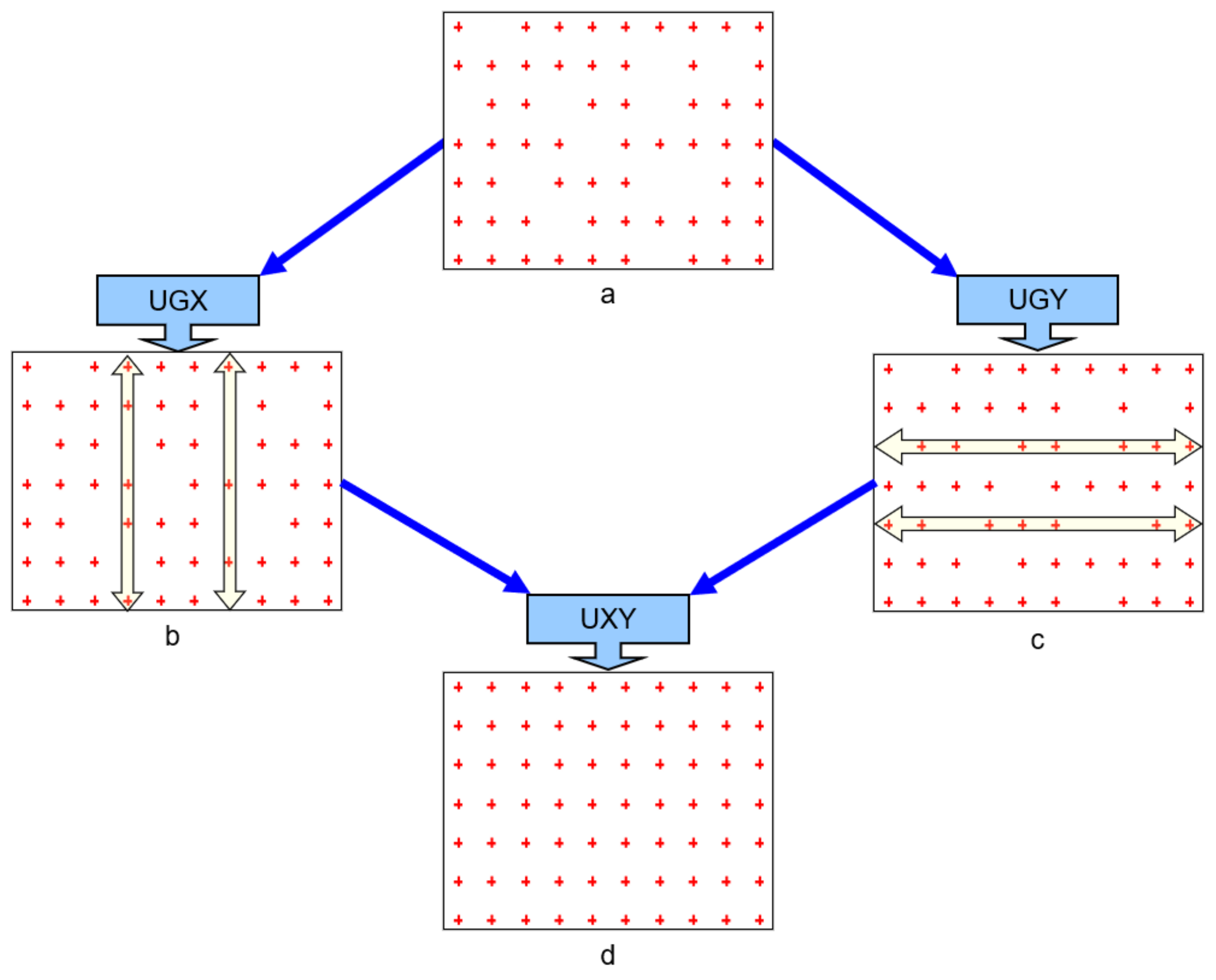
The application of the iterative method makes use of the processing for the sequence of three working modules: [UGX], [UGY], and [UXY] (Figure 2). The set with an incomplete GRID structure is used as the source data (Figure 2a). At the first stage, the [UGX] and [UGY] modules, while operating independently, generate the missing nodes in columns (the X axis direction—[UGX]) (Figure 2b) and in rows (the Y axis direction—[UGY]) (Figure 2c) of an incomplete GRID structure. At the final stage of the process, the [UXY] module merges the structures generated by the [UGX] and [UGY] modules to create a complemented (here: complete) GRID structure (Figure 2d).

The calculations are made in successive columns and rows of the analysed grid of nodes using single-variable polynomials. The file with an incomplete node structure is used as the source file in all cases. The resolution of the analysed grid of nodes is defined as the initial parameter. It can be set arbitrarily or represent the resolution of an incomplete GRID structure stored in a source file. After defining the other base distance S (Figure 1a) between the nodes, a grid with lower or higher resolution (which increases or decreases the density of the original GRID structure) can be interpolated. The inclusion of the scope of analyses enables the processing of a selected group of nodes from the original (incomplete) GRID structure. This enables the division of the entire object into arbitrary sections subject to simultaneous processing, which, in turn, allows the computational efficiency for large areas to be regulated.

Since the operation of the two modules is the same (for columns—[UGX] module, for rows—[UGY] module), their functioning in the presented methodology will be discussed with the [UGX] module used as an example. The basic task of the [UGX] module is to generate the missing nodes (located along the successive columns of the GRID structure) based on the existing nodes using a single variable polynomial of a certain degree. To this end, the structure is sorted in such a manner that the nodes in the successive columns are arranged according to the increasing coordinate x (Figure 2a). The nodes that meet the specified location criterion are then selected out of the sorted (ranked) ones. The presented methodology assumes the possibility of defining the location of the nodes involved in the approximation through the independent determination of their number before and behind the newly determined (missing) node. In addition, it is foreseen that the acceptable distance between the extreme nodes and the node being determined (in the units of resolution of the grid S denoting the spacing between the nodes) can be set. This enables the determination of the maximum size of the gap being complemented (the number of nodes to be complemented). This distance can be reduced to a specific value (a multiple of S), thus enabling the iterative complementation of the missing nodes, where gaps are complemented successfully in subsequent runs of the [UGX] module. The size of the gap being complemented can also be defined as arbitrary, which, in turn, allows the missing nodes to be determined in a single pass (without iteration). In addition, this distance (determined or calculated) is used to perform the weighting of the value being determined, which is carried out at the next processing stage. The smaller the gaps in the GRID network, the greater the assigned weight is. When the weighting option is not taken into account, all the nodes being determined are assigned the same weight, which is applicable when densifying the complete GRID structure in which the distances between nodes are identical.

Depending on the gap determined between nodes in an incomplete GRID structure, calculations are made using the approximation with a single variable polynomial of a specific degree. The source data for the determination of polynomial coefficients are the values at the nodes located (a specific number of them) in the GRID column before and behind the existing gap (Figure 2a). The calculation results are the values determined at the nodes complementing the established space. Compared to the polynomial of two variables (which generates the surface function), a single-variable polynomial enables a reduction in the number of coefficients and, thus, a reduction in the number of nodes involved in the data processing. This offers the possibility for the use of approximations in determining the missing nodes and considerably speeds up the data processing.

Any surface obtained by the interpolation process is a certain approximation of the actual surface. The adopted methodology enables the complementation of the original grid (determined by means of interpolation based on measurement points) with complementary grid nodes. The proposed method assumes the use of a properly created GRID structure, whose parameters were established in the gridding process. Missing nodes are caused by the lack of measurement points and partially by such topography (discontinuity points caused by surface faults or a technical infrastructure) that does not allow a complete grid to be generated. In the process of generating the original grid, such places are eliminated in order to obtain a continuous topographic surface. The proposed method allows the GRID structure nodes to be complemented on a continuous surface. In addition, the classical complementation of the GRID structure by a re-measurement and re-interpolation is not always feasible or cost-effective. In the absence of access to source data, the complementation of missing nodes remains the only option, with the alternative being a complete lack of data at certain locations in the area under analysis. In such cases, the proposed method enables the complementation of the node structure by means of surface approximation at the location of the missing data.

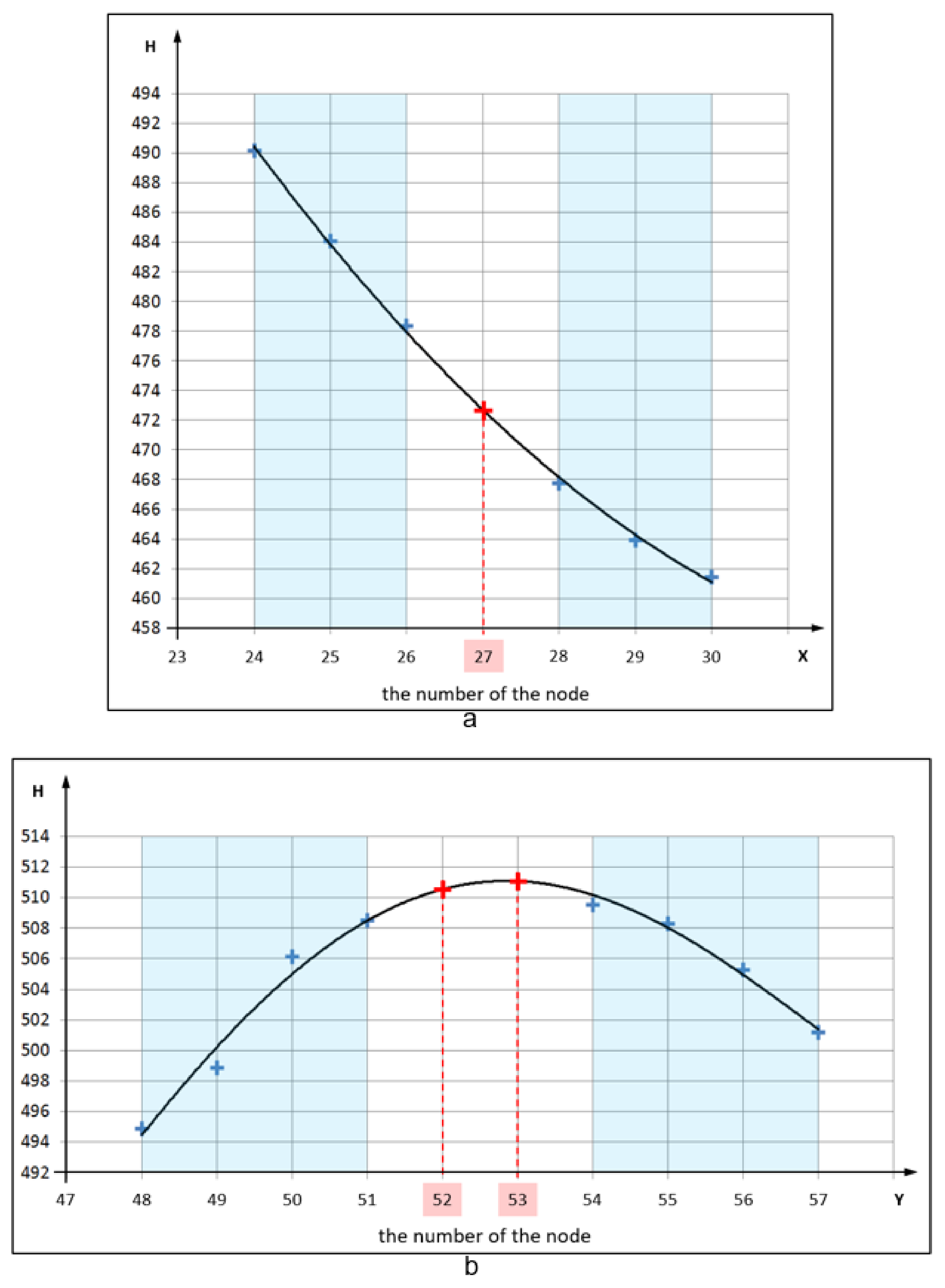
Figure 3 presents two cases of determining values at the nodes for differently defined processing parameters. The X axis is supported by the [UGX] module, while the Y axis is supported by the [UGY] module. Successive sorted nodes are located along the horizontal graph X axis, while the heights H determined at them are presented on the vertical axis. In the first case (Figure 3a), all the nodes are located in a single column of the GRID structure along the X axis. The data search space for determining the polynomial coefficients (marked in blue colour) was defined in the form of three nodes (numbers 24, 25, 26) before and three nodes (numbers: 28, 29, 30) behind the missing node with number 27 being determined. However, the acceptable distance between the extreme nodes and the node being determined (the number of the missing nodes) was set as one. The value at the node is determined by the calculation, for x, of the polynomial value as a solution of the system of equations: a polynomial of a certain degree and a straight line passing through a node with a known x coordinate.

In the methodology presented, the independent operation of the [UGX] and [UGY] modules allows different processing parameters to be defined for the columns and rows of the GRID structure under analysis. The second case (Figure 3b) illustrates the situation where the search space includes four nodes on both sides of the gap (before—the numbers 48, 49, 50, and 51, and behind—the numbers 54, 55, 56, and 57) located in a row of the ordered GRID structure along the Y axis. In this case, the acceptable distance between the extreme nodes (the size of the gap on one side or the other) is two. In this situation, both missing nodes with the numbers 52 and 53 are determined using the same polynomial coefficients. The calculations are repeated for all the defined and found location systems along each column (the [UGX] module) and each row (the [UGY] module) of the GRID structure under analysis.

In the methodology presented, the selection is envisaged (independently for the [UGX] and [UGY] modules) of the manner of determination of the degree of the polynomial whose coefficients will be used to calculate values at the nodes being determined. The polynomial degree can also be specified as constant for all the cases of the location of the nodes found in columns or rows of the GRID structure. In such a case, the determination of the node being searched for is determined by the number of existing nodal points found in the defined search space (before and behind the newly determined node). In the case of a single variable polynomial, the minimum number of points required to make calculations results from the number of equations required to solve a system of equations for a particular polynomial degree n, and is specified by relationship (1):

pw < n + 1—no solutions,

pw = n + 1—the exact solution (interpolation),

(1)

pw > n + 1—approximate solution (approximation).

where pw—number of nodal points used in the calculations; n—degree of the polynomial.

Where the number of modal points pw, found in the defined search space around a newly determined node, is too small, such a node is disregarded in the final result. On the other hand, finding a sufficient number of nodal points (1) enables the establishment of an appropriate number of equations for the polynomial of a specific degree (n), thus allowing its coefficients to be determined. This process is carried out independently for the columns located along the X axis (2) and for the rows located along the Y axis (3).

$$W\left(x\right)={\displaystyle \sum }_{i=0}^n{a}_i{x}^i$$

(2)

$$W\left(y\right)={\displaystyle \sum }_{i=0}^n{a}_i{y}^i$$

(3)

where n—degree of the polynomial; a—polynomial coefficients; x—the coordinates of the points being processed in a column (along the X axis); y—the coordinates of the points being processed in a row (along the Y axis).

The values at the nodes are complemented following the determination of polynomial coefficients (2) and (3). The number of coefficients used to calculate the values at the node being searched for is determined by the degree of the polynomial that will be used in a particular situation. These coefficients are solutions to the systems of equations created by substituting to (2) and (3) the coordinates x and y of the existing nodes surrounding the node being determined (Figure 3). Where supernumerary equations are taken into account, the solution to the system is obtained by the least squares method. The complemented value of the height of the node being determined is calculated by substituting the known coordinates x or y of a particular node (the position of the grid nodes is known thanks to the S value) to polynomials with known coefficients (2) and (3).

In addition to the possibility of setting a fixed degree of the polynomial used in calculations (independently in the [UGX] and [UGY] modules), the presented methodology also assumes the possibility of finding the polynomial that best fits the group of nodes found in the defined area (Figure 3). The extent of the search for such a polynomial can be determined by identifying its maximum degree. The maximum degree n of a polynomial (2) and (3), taken into account when calculating its coefficients, can be determined automatically. Where the maximum degree n of the polynomial is automatically determined, the number of existing nodal points found in the search space is taken into account. It determines the number of Equations (2) and (3) that can possibly be established. The process of searching for the best-fitting polynomial is carried out in successive calculation cycles while successively increasing its degree n. In order to identify the best fit, the RMS index is determined for each polynomial degree being explored (4).

$$RMS=\sqrt{\frac{1}{n}{\displaystyle \sum }_{i=1}^n{\left(f\left(x_i,y_i\right)-z_i\right)}^2}$$

(4)

where f(x_i,y_i)—the value determined from the polynomial at a theoretical nodal point with coordinates x_i and y_i; z_i—the value approximated (based on the existing nodes) at a practical nodal point with coordinates x_i and y_i; n—number of nodal points.

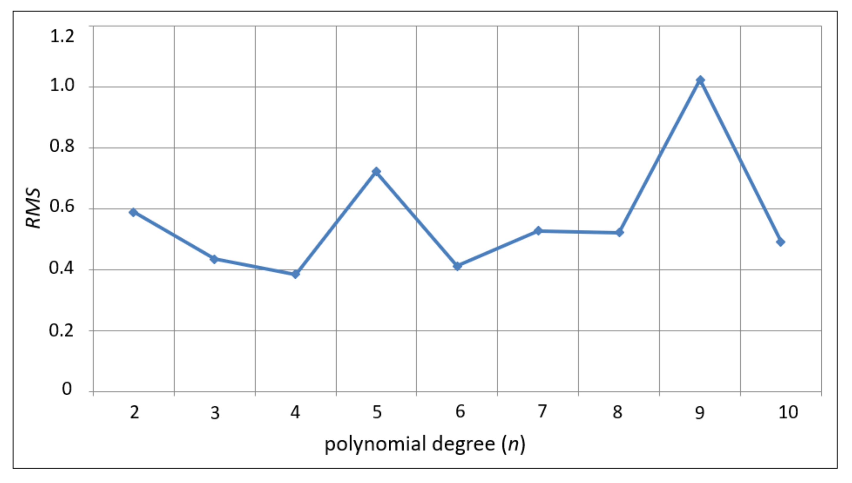
The RMS index is determined on the basis of the differences between the height of each node (involved in the approximation) and the value calculated from the solution of the system of Equations (2) or (3). Out of the analysed solutions, a polynomial is selected, for which the calculated RMS fit index is the smallest. The process of determining the polynomial degree for an example node location is shown in Figure 4. The chart shows the change in the RMS fit index for successive degrees of polynomial (from n = 2 to n = 10) with the distance between the nodes S = 5 m. In order to make the calculations, 15 nodes were taken into account in each case, which allowed an approximation solution (1) to be obtained each time.

In the presented example, the differences between the polynomials are small, except for n = 5 and n = 9. For these degrees, a deterioration in fit was noted. The best fit was obtained for n = 4, for which the RMS fit index was the smallest. For this reason, this polynomial was selected as the final solution. Where the fits of the polynomials to the source node system are comparable, the aim should be to use the approximation polynomials of the lowest possible degrees due to the occurrence of smaller distortions of the model generated with their use and the more efficient data processing process.

All the processes being discussed are implemented in the same way by the [UGX] module and the [UGY] module. The results of calculations of both modules are sets containing the missing nodes (in columns and rows) along with the value assigned to each node and specifying the size of the gap being complemented (separately for columns and rows). This value is used in the weighting process. It is the [UXY] module that is responsible for the merging of the source set with the complementary sets using an appropriate weighting of the values determined at the missing nodes (Figure 2d). Three sets are used as the source files: one file with an incomplete node structure (the original source file for the modules [UGX] and [UGY], and two files with the complementing nodes generated by the modules [UGX] and [UGY]. When merging the sets into one resulting resource, the weighting of the values at the nodes is taken into account, where the weight values are assumed to be the inverse of the second-degree power of the distance between the extreme nodes of the gap being complemented. Since the calculations are made independently for columns and rows, a portion of the nodes determined can be doubled (the value at the node being sought is set at the same location simultaneously by the [UGX] module and the [UGY] module). In this situation, the values at the nodes are also averaged with the appropriate weighting maintained. Ultimately, the resulting set is the original resource complemented by newly determined nodes whose location was defined by the [UGX] and [UGY] module processing parameters. If the structure of the nodes is sufficiently complemented, it can provide a definitive solution. Where the structure is incompletely complemented by the process described, iterative processing can be carried out in a single pass.

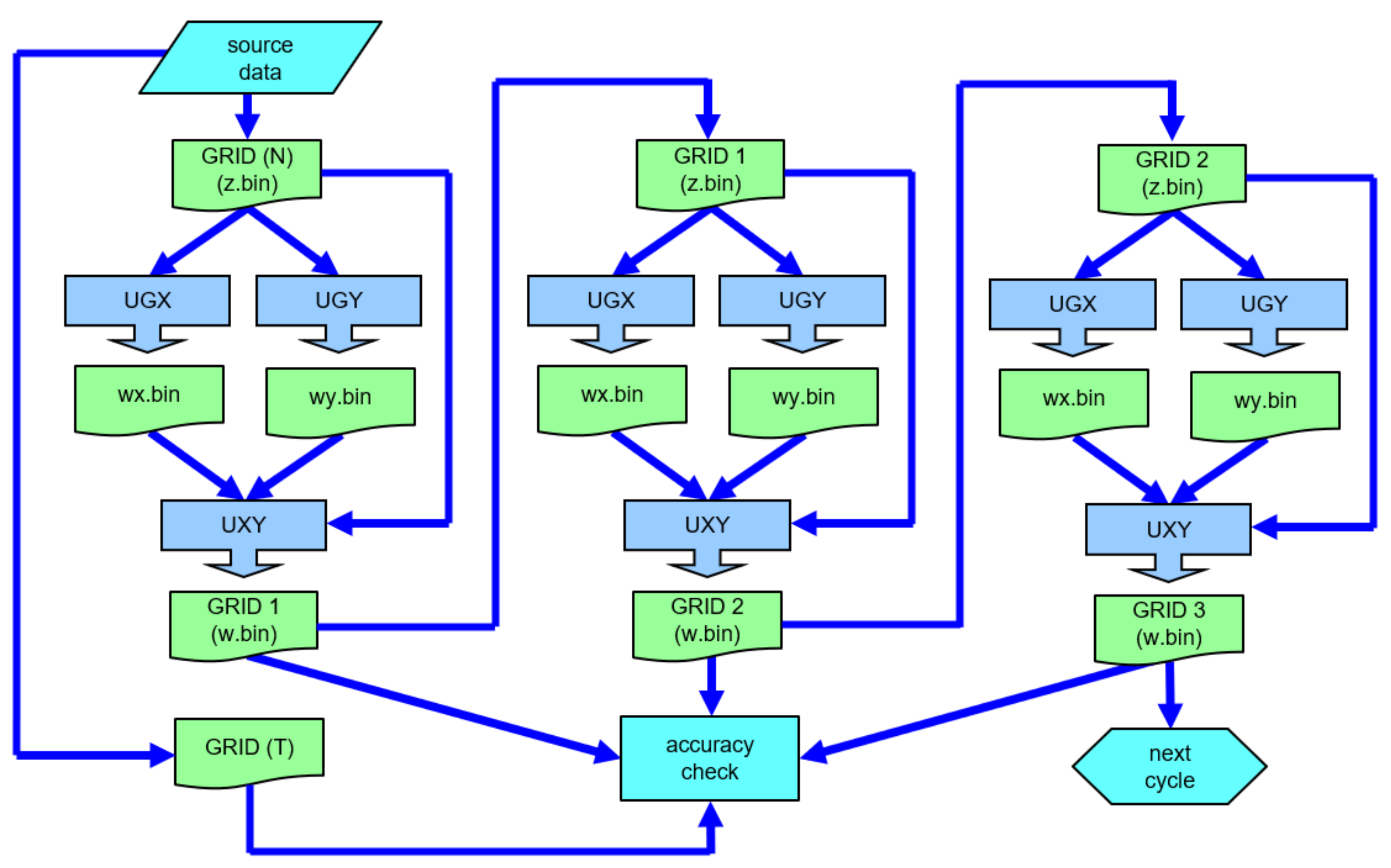
A graph showing the transfer of data in the iterative process is provided in Figure 5. In the first phase of implementation, both modules ([UGX] and [UGY]) are used, which, thanks to the possibility of parallel processing, can run simultaneously in this stage. In both cases, it is the incomplete grid of nodes (GRID (N)) that is used as the source data. The datasets used in the processing process were designated as source sets [z.bin] and resulting sets [w.bin] (Figure 5). The [UGX] and [UGY] modules, operating independently, each time generate the missing nodes in the GRID structure stored in the source file [z.bin]. In each iteration of the processing process, independent resulting files with the missing nodes are created: [wx.bin]—for the GRID columns and [wy.bin]—for the GRID rows. Each time, they can be generated for other criteria defined individually for each iteration.

The resulting data of a specific iteration are transferred to the next iteration and constitute the source data for it. At each stage of processing, the resulting data can be subjected to an accuracy check. The iterative process is terminated when all the missing nodes of the GRID structure have been generated. It can also be terminated at the moment when the surface model created in the next iteration is inferior to that of the previous iteration.

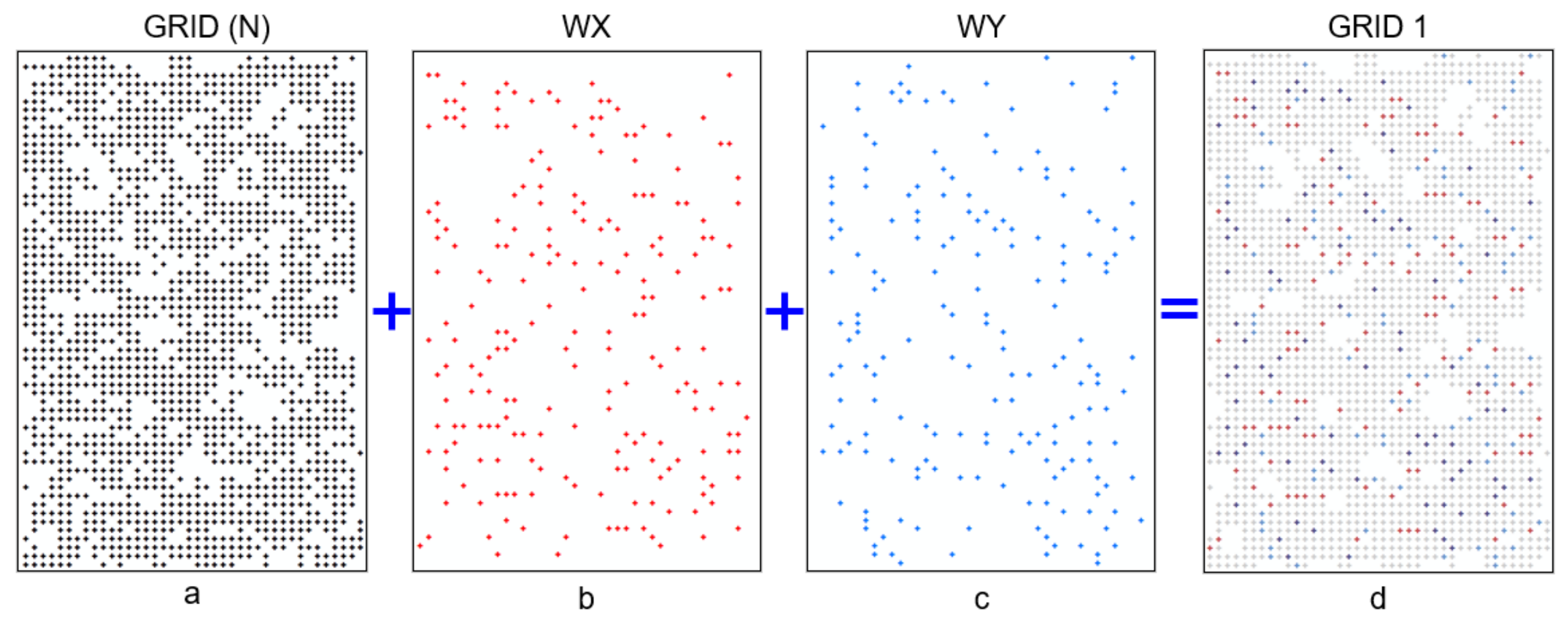
Figure 6 shows the successive stages of complementing the grid of nodes when carrying out one iteration. The criterion for finding nodes for polynomial approximation (two nodes before the found gap and two nodes behind it) as well as for the location of nodes to be determined (a maximum of a single missing node) was established identically for the modules [UGX] and [UGY]. The two modules, operating simultaneously on the same source dataset (GRID (N)—Figure 5 and Figure 6a), generated nodes with the location shown in Figure 6b (the WX set created by the [UGX] module—red colour) and Figure 6c (the WY set created by the [UGY] module—light blue colour). These independently complement the nodes in columns (WX) and rows (WY) according to the same criterion (one missing node). At the next processing stage, the two generated files (after appropriate weighting) were merged with the source file using the [UXY] module to form one resulting resource (GRID 1—Figure 5 and Figure 6d). The overlapping nodes (i.e., those generated at the same time by both modules at the same place) are marked in dark blue (Figure 6d). The values determined at these nodes were averaged.

The visible gaps in the resulting node structure (Figure 6d) were not complemented due to the adopted location criterion (a single missing node). If the generated surface model meets the assumed requirements, such a structure can be considered the final solution. However, when the aim is to obtain a complete GRID structure, the next complementation of the missing nodes needs to be carried out in subsequent iterative processes.

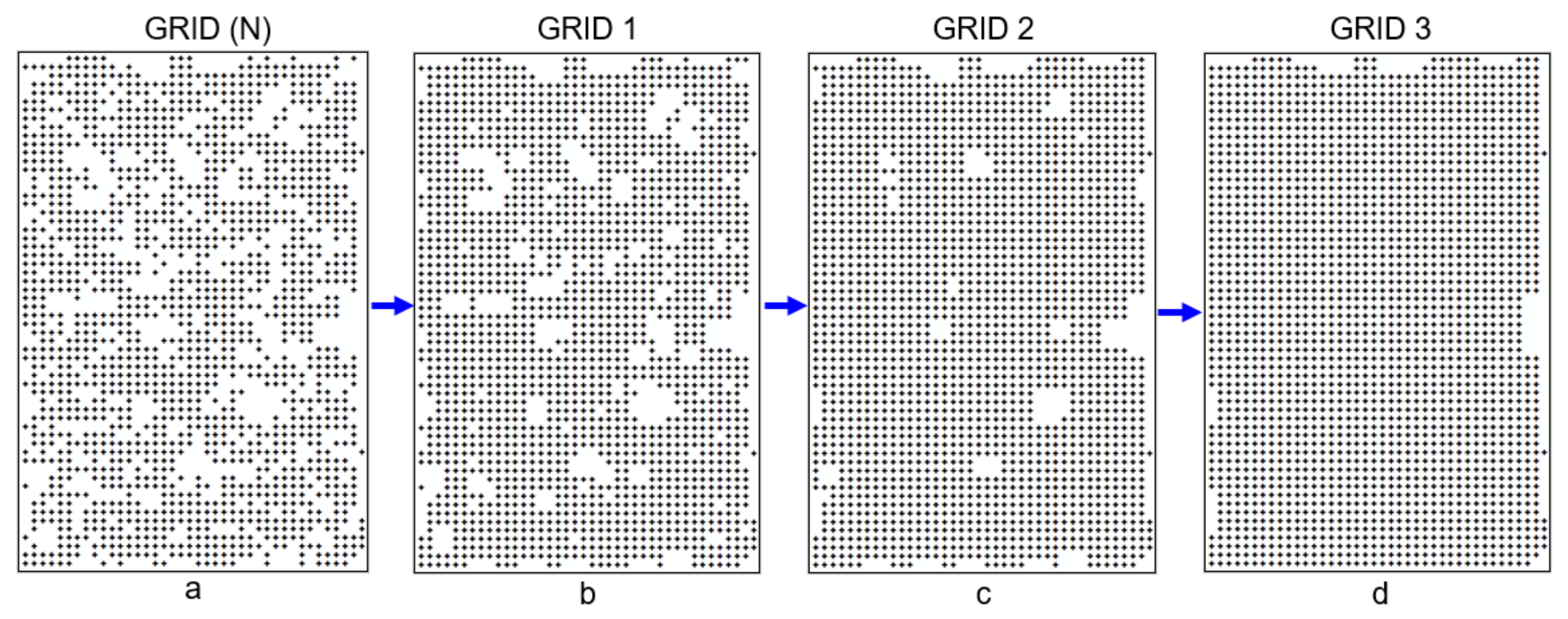
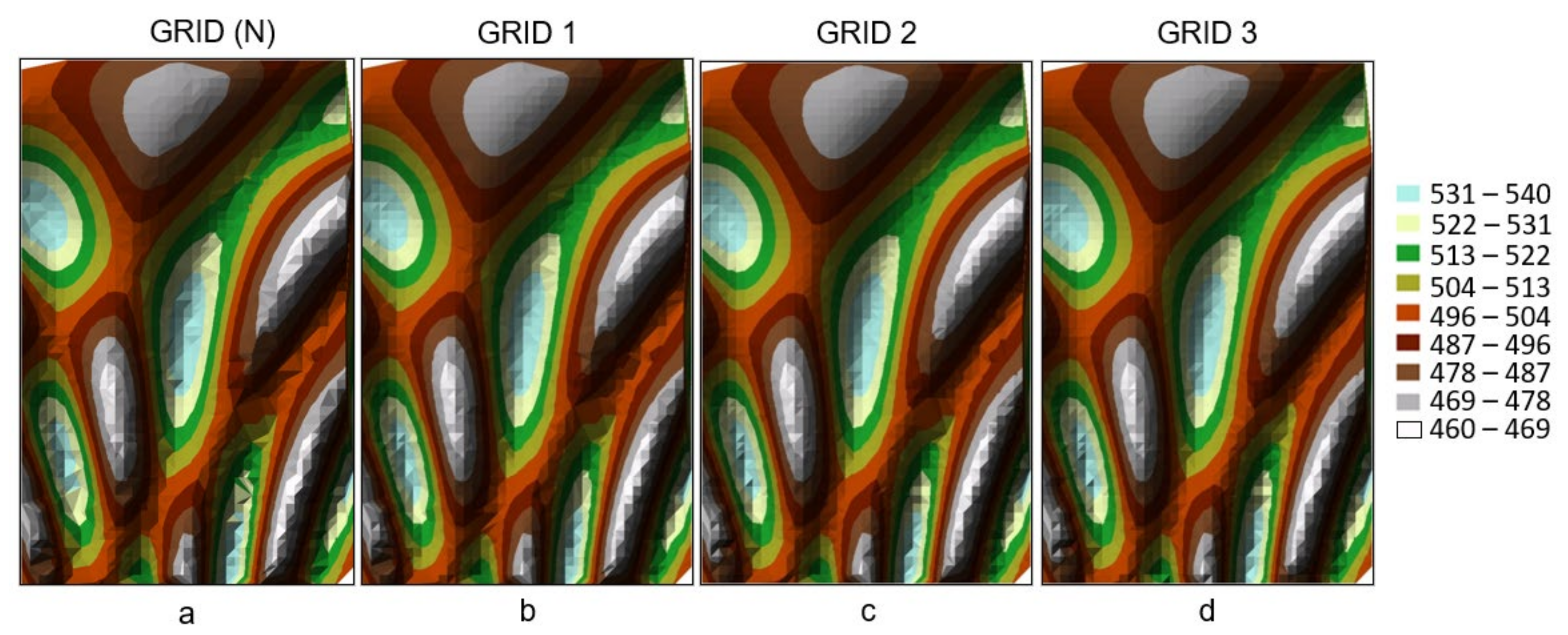
The stages of complementing the GRID node structure in successive iterations are shown in Figure 7. In the presented process, a resulting set of nodes (GRID 1—Figure 6d and Figure 7b) is generated in the first iteration based on the original resource (GRID (N)—Figure 6a and Figure 7a). This set becomes the source set for the next iteration (Figure 5). The location parameters defined in the introduction of the modules [UGX] and [UGY] can remain the same for all iterations. However, maintaining the same processing parameters (a maximum of one missing node) for successive iterations does not result in the full complementation of the missing gaps in the GRID structure (Figure 6a). Therefore, the entire processing process needs to be repeated for differently defined location parameters. The next iteration established three nodes before the found gap and three nodes behind this gap (as the data for polynomial determination), and a maximum of two newly determined nodes to be complemented in the row and column in the newly created GRID structure. The result of running the [UGX], [UGY], and [UXY] module sequence with the node location parameters defined in this manner enabled the generation of a GRID 2 network of nodes (Figure 7c) in the next iterative process (Figure 5).

In the further process, this set can represent the final solution or be used as the source data for the next iteration. In the presented case (Figure 7), the processing process was repeated for the next group of nodes found at differently defined location parameters. The next iteration adopted four nodes before the found gap and four nodes behind that gap as the data for determining the polynomial coefficients, and a maximum of three nodes to be determined in the newly created GRID structure. This enabled the generation of the GRID 3 structure (Figure 7d) based on the GRID 2 structure (Figure 7c) in the next iterative process (Figure 5). The process of iterative complementation of the missing nodes is repeated until the used sequence of [UGX], [UGY], and [UXY] modules stops generating results. This occurs when the missing nodes are not determined for the chosen processing parameters, i.e., the last generated GRID does not differ in the number of nodes from the penultimate one. Processing is then stopped, and the last GRID set is regarded as the resulting one. The final resulting GRID 3 structure (Figure 7d), presented in the example, has fully complemented internal nodes.

The ultimate effectiveness of the presented processing is determined by a number of factors, which include the morphological diversity of the surface, the number and density of measurement points, the determined resolution of the GRID being created, and the applied original grid interpolation algorithms. On the other hand, the number and size of the gaps formed in the computational spectrum, as well as the number of iterations used, have a direct effect on the effectiveness of the presented methods. The single-pass method is as quick as one iteration in the iterative method. The number of iterations is determined by a stage check, during which it is determined whether the DTM model is already sufficiently accurate.

At each stage of creating intermediate sets (at the end of each iteration), an accuracy check (Figure 5) is available, which can ultimately verify the quality of the surface models being generated. Performing checks at each stage allows the processing to be stopped if increasingly poor results are generated in successive iterations. In general, in order to maintain the model accuracy, the aim should be to provide the minimum acceptable gap between the extreme nodes (the minimum number of nodes to be determined in a single iteration). The application of the iterative process is always preferable to generating the missing nodes in a single pass (setting high tolerance in the parameters qualifying the nodes for calculation). This particularly applies to morphologically diverse areas. Where surfaces are less diverse, greater tolerance can be applied in the selection of distances between extreme nodes.

Moreover, with a large number of missing nodes, it is not always possible to obtain a complete GRID structure. Setting a large value of the maximum gap tolerance (the number of nodes to be complemented) with large gaps in the original structure creates areas in which generating the missing nodes is not possible. Figure 8a shows an incomplete grid of nodes (black colour), while Figure 8b shows the complementary structure (red colour). Setting the maximum tolerance at the level of seven nodes to be determined in the newly created GRID structure did not allow a complete grid to be generated due to the gaps in the source set being too large.

The GRID structure can be created based on various measurement data (LiDAR, MBES, aerial photographs). As regards source materials, where large gaps are found in the measurement spectrum, a complete GRID network cannot be determined. This is related to the determination of the structural parameters of the GRID structure, which enables the determination of the location of the grid of interpolated points as well as its resolution, depending on the density of measurement points, the morphology of the surface being measured, or the gaps formed due to the elimination of the technical infrastructure. This creates a situation where, due to the lack of measurement points, a complete, sufficiently accurate GRID structure cannot be obtained by any of the methods under consideration. In such a case, the re-measurement of the missing points by another mass measurement method should be considered. If the GRID network determination was carried out using aerial photographs, the unrecorded measurement areas can be complemented by a LiDAR measurement. The missing areas can also be partially covered using classical tachymetric or GPS methods.

Where large gaps are found between nodes, complementing them by one of the available interpolation methods may be considered. In practice, classical interpolation methods (Spline Functions, Radial Basis Function, Kriging) are most commonly used to determine a grid of nodes based on the measurement points [43,44,45]. These methods can also be employed to complement missing nodes in the GRID structure. However, the application of these methods to complement missing nodes is associated with certain limitations. In most cases, classical surface interpolation methods require a large number of points that should be distributed close to and around the node being searched for. Where the existing nodes are used as data for the next interpolation, this condition is not fulfilled because there are few points, and the nearest nodes are located at a relatively large distance (multiples of the base distance between the nodes). Furthermore, the classical methods determine the values being searched for in a single computational run, which, in the case of large gaps, results in lower accuracy. In this process, an entire model is obtained immediately, and there is no stage check. Local distortions of the surface are often generalised, and the selected interpolation method has the same parameters over the entire area. The described method uses different degree polynomials of one variable, which allows the number of nodal points involved in the interpolation to be minimised, and the degree of the polynomial to be fitted to their number. The iterative variant of the method under consideration enables the successive complementation of missing nodes with the possibility of changing the interpolation parameters at each stage. This enables the application of a check on the accuracy of the models being generated at each interpolation stage. In this way, the interpolation parameters can be selected according to the specific characteristics of local distortions without generalising the method parameters over the entire surface. The discussed methodology also includes a single-pass variant (faster but less accurate), which is comparable to classical surface methods. The limitation of this method is the occurrence of large gaps in the original GRID structure. This variant of the method can be used for surfaces that are flat or not very morphologically diverse. In all other cases, the application of the iterative method is preferable.

Thanks to the application of the iterative method, it is possible to successively complement the GRID structure in successive processing cycles. This enables the provision of a definition of the individual processing parameters in each cycle and the generation of precisely defined groups of nodes complementing the structure in each stage. However, it is not always possible to create a complete grid, as the generation, in the iterative process, of all the missing nodes in the situation concerned (few source nodes) leads to too much distortion of the model. As regards large shortages in the original GRID structure, this method can be applied to determine the potential areas in which nodes cannot be generated.

3. Results

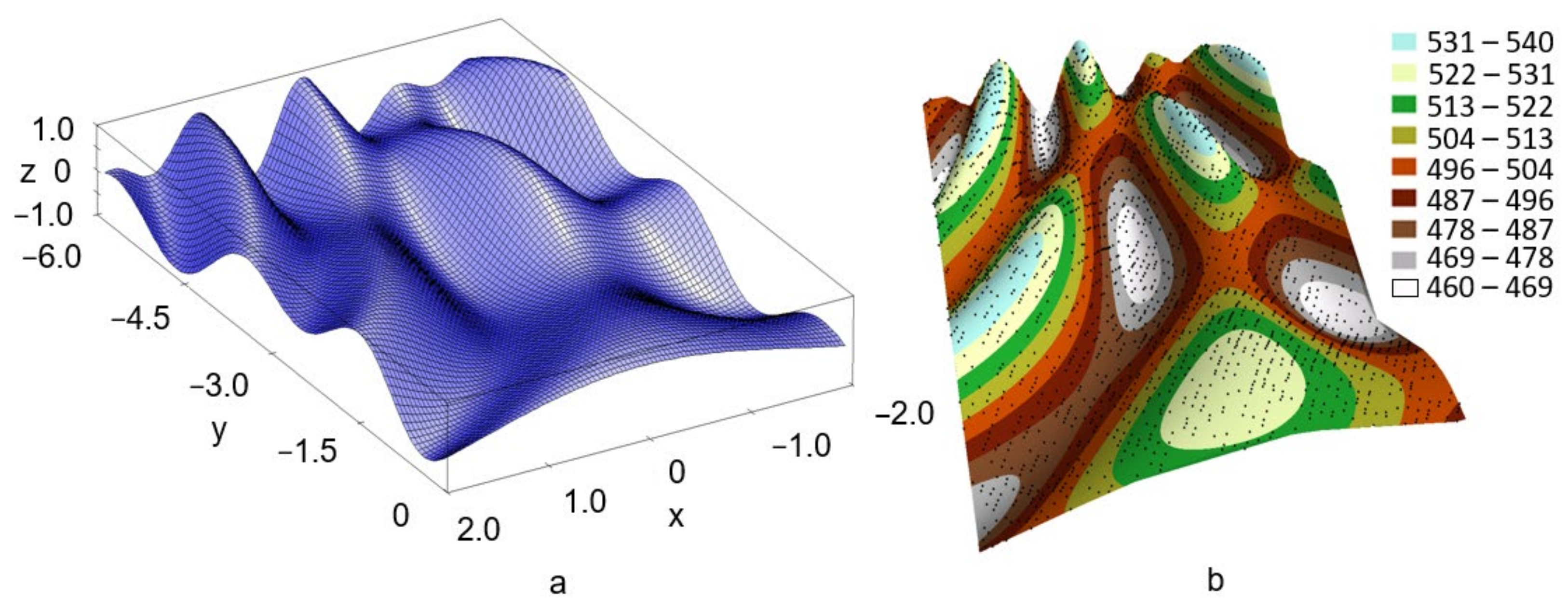
In order to analyse the quality of the models generated using the two methods for determining the missing nodes in the GRID structure (iterative and single-pass), a theoretical model was used, along with several examples of node complementation in the actual surface models. A surface model generated by a function of two variables was used for a comparative analysis of the differences between the practical surface (created by interpolation) and the theoretical surface (determined from the function). This approach allows pseudo-measurement points to be generated at any location and height values to be obtained for them based on the function. Based on these points, a practical GRID structure is generated in the interpolation process and then complemented by the described method. The same function is also used to obtain height values at the locations where the nodes of the theoretical GRID structure will be determined. A comparison of values between the nodes of the practical and theoretical structure is used to analyse the fit of both surfaces and determine the accuracy. In order to create a theoretical model, the function of two variables (5) was used, on the basis of which the surface forming a theoretical test model shown in Figure 9a was generated.

$$\begin{gathered} f\left(x,y\right)=cos(xy+e^x)cos(x-y) \\ x\in \left[-2,2\left],y\in \right[-6,0\right] \end{gathered}$$

(5)

The test model enabled the generation of pseudo-measurement points that created a virtual workspace (Figure 9b). The working area was scaled to a rectangle with sides of 400 m × 600 m and shifted in relation to the system axis in such a manner that all working points had positive coordinate values and the maximum vertical height differences in the model did not exceed 70 m. The pseudo-measurement points were distributed in a manner that simulated a LiDAR measurement. The angle of the row in relation to the horizontal Y axis was 50°, the distance between rows was 7 m, the distance between points in a row was 3 m, and the maximum error of the position of pseudo-measurement points was the same in relation to all the axes, and amounted to 0.10 m. In order to reduce the number of pseudo-measurement points used in the interpolation, 30% of the points representing the source set of the points used in further calculations were selected from the original set (Figure 9b). The working model parameters were carefully selected to present the possibilities of the methodology presented for the case of reduced data quality (e.g., a measurement performed by LiDAR in a submontane forest area, and the data resource filtered to eliminate the signal beams reflected from trees). A model generated on the basis of pseudo-measurement points selected in this manner is presented in Figure 10a. The surface morphology used (relatively large height differences within a small area) and the reduced number of pseudo-measurement points did not allow an accurate model to be created.

The GRID structure nodes were then interpolated using such a resource of pseudo-measurement points. The grid resolution (the spacing S between the nodes) was set at 10 m, and the search for pseudo-measurement points for interpolation was performed within a radius of 15 m. Four sectors were used as the method for searching points for the interpolation, while for the interpolation, an algorithm using radial basis functions was used [70,71]. In the resulting file of the interpolation, only the nodes with correctly located pseudo-measurement points were retained, while the remaining nodes were rejected. The reduced number of pseudo-measurement points prevented the determination of values at all the nodes, and finally, an incomplete GRID (N) node structure shown in Figure 7a was created. The interpolation model created on the basis of GRID (N) is shown in Figure 11a. In order to compare the quality of the models, the model generated on the basis of the theoretical node structure (GRID (T), S = 10 m), used for the processing accuracy check, is shown in Figure 10b.

The following figures (Figure 11) show interpolation models generated on the basis of a successively complemented GRID structure in the process of previously described iterative processing methodology. The surface models from Figure 11a–d correspond to the successive node structures presented in Figure 7a–d. The presented iterative processing process performs, in successive steps, the successive approximations of the surface under analysis, which contributes to the generation of increasingly better models. This results from the fact that, in each successive step of iterative processing, the structure is complemented with a small number of nodes resulting from the defined processing parameters. Checking on the acceptable gap between the nodes (in each row and column of the newly created structure) while performing the successive iterations enables the increase in the accuracy of the finally generated model in relation to the model created on a single-pass basis.

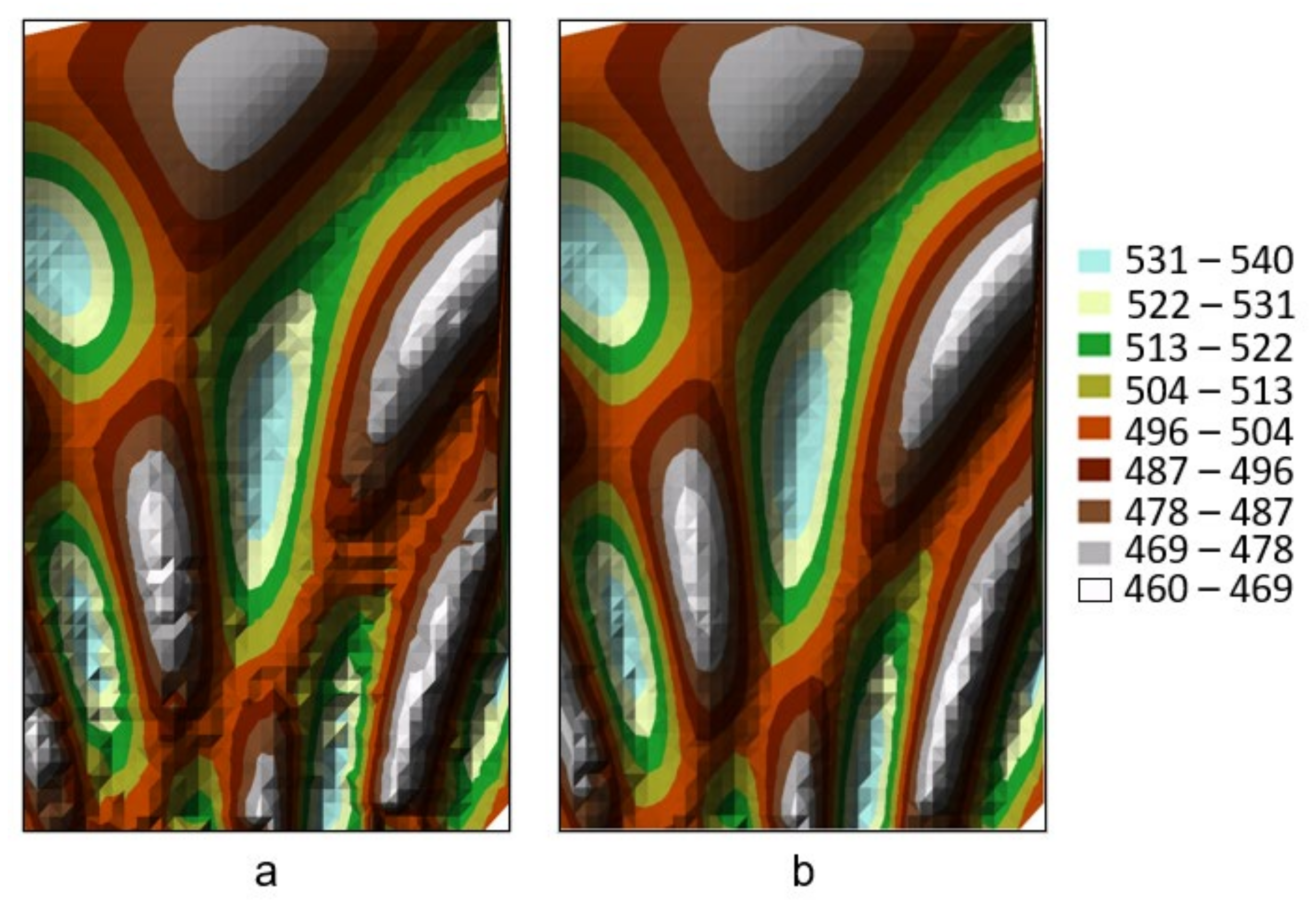
A comparison of the models generated on the basis of the same incomplete GRID structure at different processing parameters is presented in Figure 12. In the first case, the model was generated by the single-pass method, where an arbitrary number of missing nodes in columns and rows were defined (Figure 12a). This enables the model to be generated very efficiently while reducing its accuracy. The model generated in this manner shows local distortions, located in particular in the most morphologically diverse area. However, low-diversity areas are characterised by small deformations. This method can be applied to surfaces with small local height differences where it is sufficiently accurate. In the second case (Figure 12b), the model was generated by the iterative methods, which checked the size of acceptable gaps in the structure of nodes in each cycle (according to the workflow shown in Figure 5). This ultimately allowed a more accurate model to be obtained, particularly in an area with greater morphological diversity.

A geometrical analysis of the surface of the resulting (practical) object can be carried out by means of a comparison with a theoretical (functional) model by applying differential diagrams. They allow the degree of spatial distortions to be assessed over the entire surface of the object. The greater the difference between the practical and theoretical models, the greater the values shown in the diagrams. For an indicative assessment, the RMS coefficient (4), which enables an assessment of the fit of the practical and theoretical surfaces using a single value, can be used.

A comparison of the accuracy of the interpolation models is made in Figure 13. The presented differential graphs were created on the basis of the GRID (T) theoretical model generated from function (5) (Figure 10b). These show the absolute value of the difference in values at each nodal point of the GRID structure. This difference results from subtracting the theoretical value GRID (T) (obtained from function (5)) from the practical values (obtained directly from the interpolation—GRID (N), and after the iterative complementation—GRID 3). The differential graph generated for the model with an incomplete GRID (N) node structure (Figure 7a and Figure 11a) is shown in Figure 13a. Figure 13b shows a differential graph generated for the final complemented GRID 3 structure (Figure 7d and Figure 11d) created in the iterative process being described (Figure 5). Above the charts (Figure 13), the RMS index (4) was provided, which enables the assessment of the degree of fit between the two models and the theoretical GRID (T) model (Figure 10b).

The analysis of the two differential graphs reveals an improvement in the quality of the surface of the model generated in the iterative process (complete GRID 3) (Figure 13b) as compared to the original model (incomplete GRID (N)) (Figure 13a). The improvement in the surface fit is also indicated by the smaller value of the RMS index obtained for the GRID 3 model.

4. Discussion

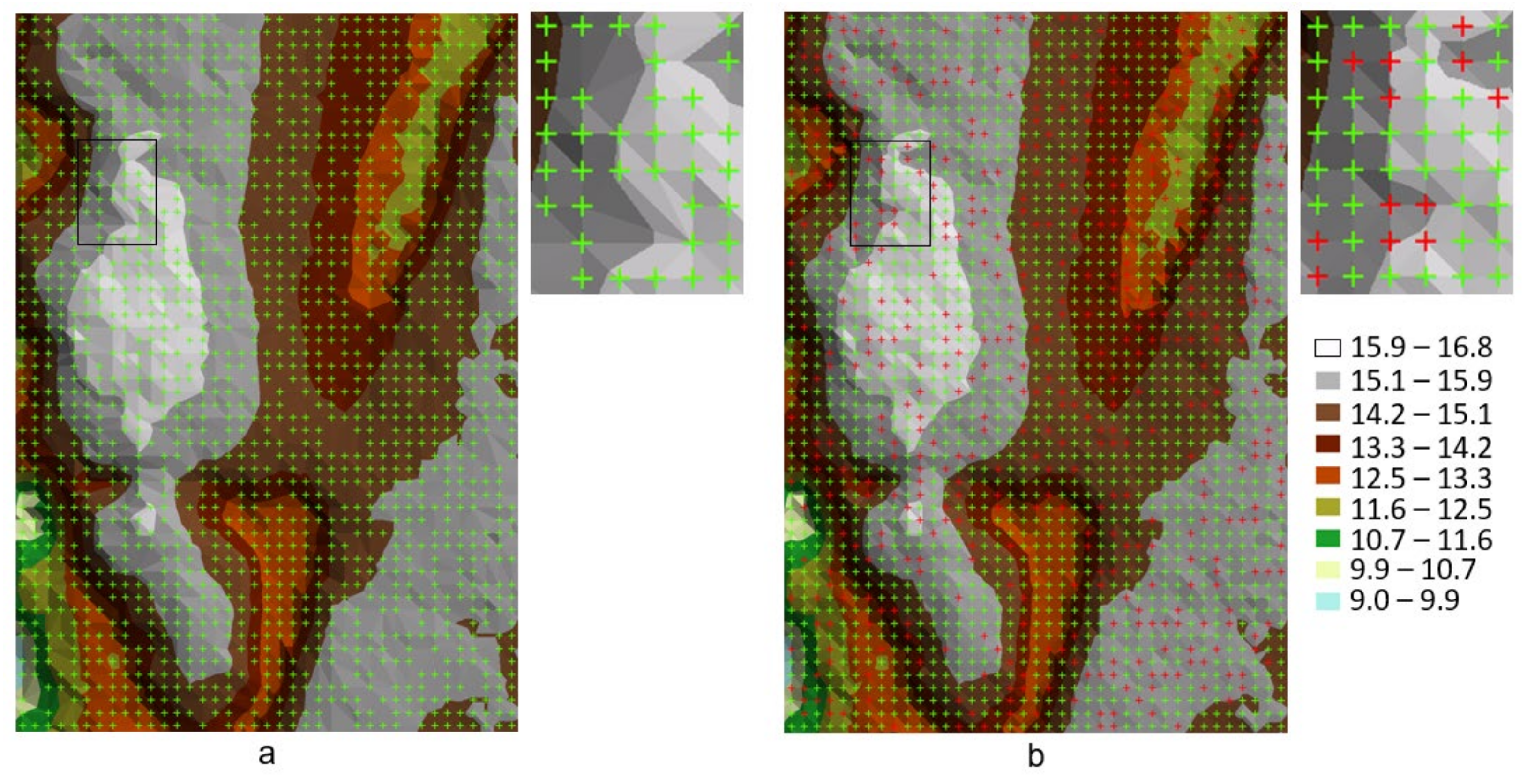
The presented methodology for the procedure was also tested on the actual terrain models (DTM) measured using a LiDAR scanner. Figure 14a shows a surface model created on the basis of an incomplete node structure (green colour). The nodes with 2 m resolution were generated on the basis of measurement points distributed in rows located at an angle of 65° in relation to the horizontal Y axis. The distance between rows was 3 m, while the distance between points in a row was 1 m. The error in the position of the measurement points in the direction perpendicular to the row was 0.10 m, in the direction parallel to the row was 0.05 m, and the height measurement error was 0.15 m. For the interpolation of values at a node, an opposing triangle field balancing algorithm was applied, which only used the measurement points found within a radius of 2 m by the four-sector method [72,73]. The location of the measurement points prevented the generation of a complete GRID structure. The DTM model created on the basis of such a structure shows areas of deformation located where nodes are missing, which prevents the generation of the proper morphological shape in these zones (Figure 14a). The enlarged part of the model shows an example of such a deformation.

The values of the missing nodes were then complemented by the iterative method described in the methodology presented. These values were determined using interpolation polynomials (2) and (3), whose coefficients were calculated using the described modules [UGX] and [UGY]. Two nodes were set before the found gap and two nodes behind this gap, with a maximum of one node being determined that complements the missing gap as the processing parameters in the [UGX] and [UGY] modules. After completing four iterative cycles, the missing nodes were totally complemented (red colour), and a complete GRID structure was generated (Figure 14b). The surface model created on the basis of the complete grid exhibits smaller local distortions. The enlarged area shows the same part of DTM as in the previous case. The generated additional nodes complement the existing gaps in the original GRID structure and allow the generated model quality to be increased. The model with complete grid of nodes can be used to compare the processed data in different measurement epochs.

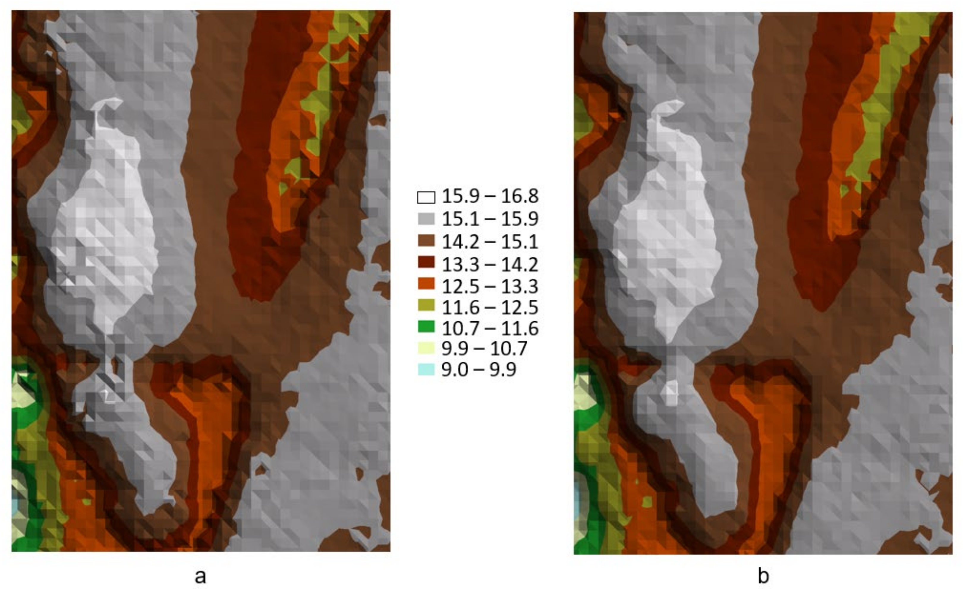
In order to compare the quality of models created by the single-pass and iterative method, Figure 15 shows two surface models generated on the basis of the same incomplete GRID structure (Figure 14a). In the first case (Figure 15a), DTM was generated on the basis of the original GRID structure complemented to a complete grid with nodes determined in a single cycle (on a single-pass basis). In this case, the described [UGX] and [UGY] modules were used, for which the determination of any number of the missing nodes in each column (X axis) and row (Y axis) was established. What can be noticed are the local distortions of the surface, particularly in zones of high morphological diversity. In the second case (Figure 15b), the model was generated in three iterative cycles (Figure 5) in stages with the previously described parameters (Figure 7). An improvement in the model quality is particularly noticeable in the zones with diverse local height differences.

The correctness of the generated DTM model can be checked by several methods. In view of the number of points being generated, the best results are obtained by comparing them with another DTM model generated at an even greater density of measurement points. However, this method is not always feasible and cost-effective. The presented DTM example was checked based on a GPS-RTK measurement at locations where missing nodes were generated. The height accuracy of the complementary nodes was at an accuracy level equal to the original nodes. A geodetic control network and the already measured technical infrastructure can also be used to check the measurements taken in urbanised areas.

The presented node grid complementation methods can also be employed to increase the resolution (density) of the existing GRID structure (whether complete or not). To this end, the node structure created using one of the methods described can be used as well. In the case of the application of the module sequence [UGX]–[UGY]–[UXY], in the [UGX] and [UGY] module processing parameters, the target resolution of the structure being generated, e.g., S2 = 1/N·S (where N is the denominator of the fraction reducing the S value, and S is the distance between the nodes) should be defined as the spacing between the nodes of the GRID network being generated. In order to increase the resolution, the resulting S2 value is lower than the original S value. Additionally, when increasing the resolution of the complete GRID structure, the process of determining the missing nodes can be carried out more efficiently by abandoning the weighting of the results. All the nodes being determined are assigned the same weight, as the distances between the nodes are the same. The other processing parameters are determined by the resolution of the original node structure. In the iterative process of the module sequence (Figure 5), a grid of nodes with an assumed resulting resolution is ultimately generated.

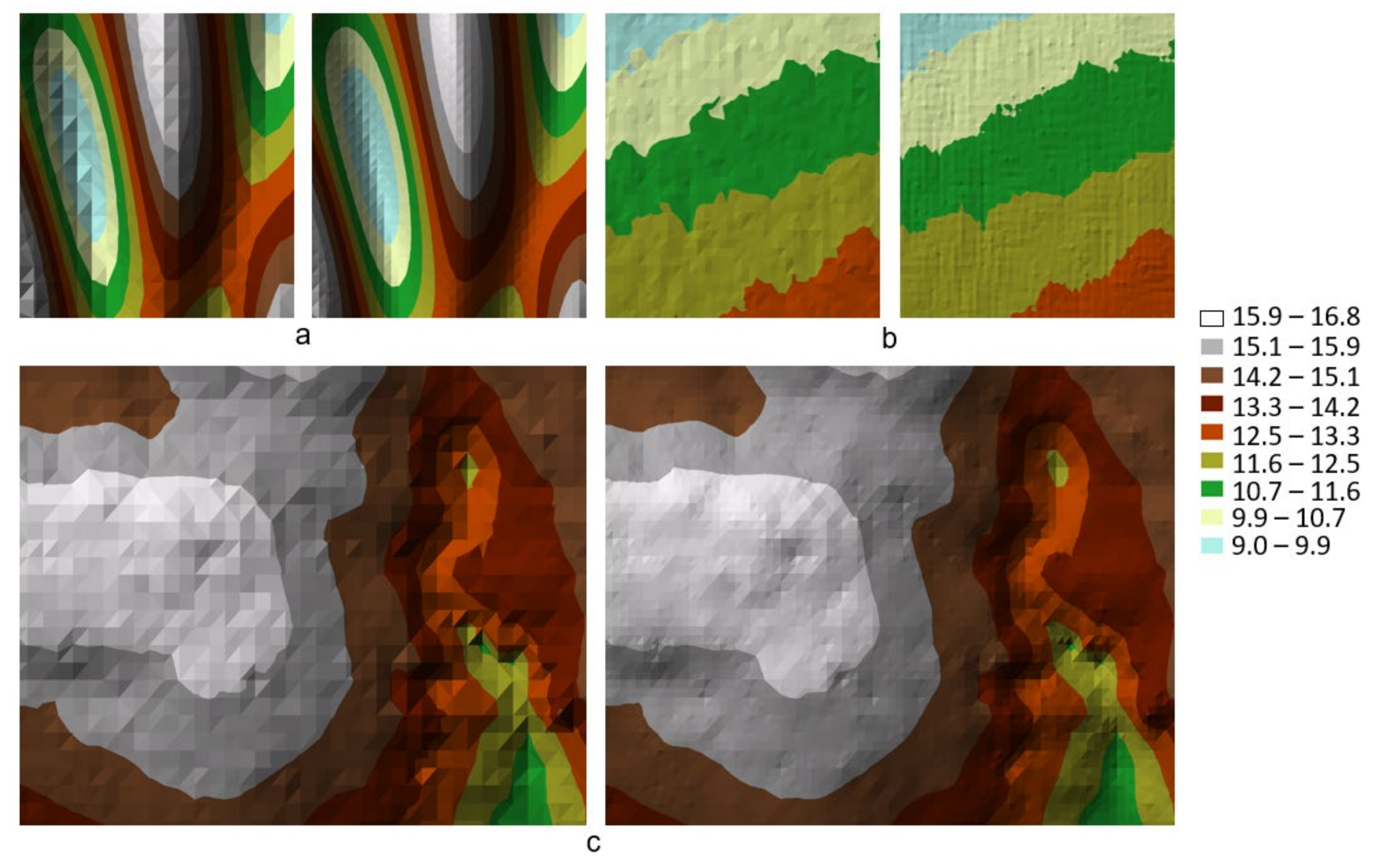
The application of the discussed methods is presented in Figure 16, with the increasing resolution of a complete GRID structure provided as an example. The first case (Figure 16a) shows a single-pass determination of the missing nodes and an increase in the GRID resolution (from S = 4 m to S = 2 m) in a single cycle of the sequence [UGX]–[UGY]–[UXY] running on a theoretical model. In this case, an improvement in the quality of the model is evident. In the second case (Figure 16b), the low-diverse DTM surface was processed by the iterative method. In this case, the model resolution was increased two times (from S = 10 m to S = 5 m), which allowed a more accurate surface to be obtained on the area with a low height difference. In this model, a characteristic structure of the generated surface, resulting from the large original S value, is noticeable.

The third example (Figure 16c) presents the case of the use of the sequence [UGX]–[UGY]–[UXY], operating iteratively, to increase the resolution of the GRID structure (from S = 2 m to S = 1 m) on a DTM model with a varied morphological surface. In this case, increasing the GRID resolution results in the smoothing of the generated DTM surface, with the newly created surface containing no local distortions characteristic of the original GRID structure.

The method presented in the study shows one of the many aspects that arise when creating a DTM based on mass measurement data. In order to carry out various analyses, the processing parameters can be defined in a number of ways. By applying the method in question, the original GRID with a different resolution of the base GRID network, generated at a different density of measurement points, can be used. In order to create the original structure, various interpolation algorithms can be used, and each algorithm can have different processing parameters (different search radii of measurement points, division into different search sectors, a specified number of measurement points involved in interpolation, the variable parameters of the interpolation or approximation functions, etc.). The study provides examples of the application of the technology in question on two theoretical models and four practical models. Practical models were selected to include areas with different surface morphologies. This enables the presentation of the varying effectiveness of the method in areas with a more and less diverse surface morphology. The principle of node complementation is universal for different surface models: terrain models, bottom models, or engineering structure models. The methods under consideration can be employed wherever a surface has been measured using a point cloud (LiDAR, MBES), and a GRID structure can be generated on its basis.

5. Conclusions

The application of the described methodology enables the generation of the missing nodes in an incomplete original GRID structure, thus allowing a partly or totally complemented resulting structure to be created. Under the methodology concerned, the accuracy of the models created by the single-pass and iterative operation of computational modules was compared. The analysed variants of complementing the GRID structure nodes indicate the advantage of the iterative method. The iterative method enables the GRID structure to be successively complemented in successive processing cycles. Thanks to this method, the successive approximations of the surface being processed are carried out, and the GRID models are increasingly complete. The application of a control check following each iteration enables the solution of the most favourable variant from among the newly generated DTM models.

The application of the iterative process, particularly in morphologically diverse areas, is a better solution than generating the missing nodes in a single pass. This is achieved, however, during a more complex and less efficient computational algorithm. The more efficient single-pass method, on the other hand, is applicable to low-diverse areas where the accuracies obtained are comparable to the iterative method. While the single-pass method (for morphologically diverse surfaces) actually allows a model to be generated very efficiently, it reduces its accuracy. Moreover, large shortages in the original GRID structure sometimes prevent the complementation of the missing nodes. As regards large shortages in the original GRID structure, the described methods can be applied to determine the potential areas in which nodes cannot be generated.

Thanks to the specification of the location of the nodes involved in the approximation and the determination of the acceptable distance between the extreme nodes and the node being determined, it becomes possible to regulate the accuracy of the newly created GRID structure. In the method described, the aim should be to provide a minimum gap between the extreme nodes, as it contributes to a reduction in the polynomial degree and an increase in the calculation accuracy. On the other hand, the automated method for determining the maximum degree of the polynomial involved in calculations allows the best quality digital terrain model to be obtained. When selecting the polynomial fit, the aim should be to use approximation polynomials of the lowest possible degree. Such polynomials, while enabling the approximation of values in the newly determined nodes, increase accuracy and computational efficiency.

The described methodology can also be applied to increase the resolution of the already existing grid of nodes. This process can be used to smooth the generated DTM created on the basis of the GRID structure and contributes to the elimination of characteristic block surface faults and disturbances in the contour line course. The advantage of the methods described is the fact that the overall shape of the surface being smoothed is preserved because the nodes of the original GRID structure (source files) do not change their location in space.

Satisfactory results can be obtained with the presented methodology when complementing the accurately determined original GRID structure. Such a structure should be determined on the basis of a sufficient number of properly located measurement points while excluding the cases of extrapolation. The use of an accurate GRID structure for the iterative determination of the missing nodes yields better results than the interpolation of a complete grid based on the incorrect location of the measurement points (which do not surround the node or are too distant). Moreover, the missing nodes can be determined, or their resolution can be increased in a situation where measurement resources are not available. An additional advantage of such data processing is its high efficiency, which is particularly important for LiDAR-derived data. Moreover, complementing small shortages in the GRID structure in the case of the methods discussed is more profitable economically than performing a new interpolation for the measurement resources. The application of the assumptions of the methodology described enables the generation of a complete GRID structure, which contributes to increasing the DTM quality and can be used for data processing in successive measurement epochs while allowing the changes in the DTM model to be analysed over time.