Near-Surface Wind Profiling in a Utility-Scale Onshore Wind Farm Using Scanning Doppler Lidar: Quality Control and Validation

Abstract

Wind profiling within operating wind farms is important for both wind resource assessment and wind power prediction. With increasing wind turbine size, it is getting difficult to obtain wind profiles covering the turbine-affecting area due to the limited height of wind towers. In this study, a stepwise quality control and optimizing process for deriving high-quality near-surface wind profiles within wind farms is proposed. The method is based on the radial wind speed obtained by the Doppler Wind Lidar velocity-azimuth display (VAD) technique. The method is used to obtain the whole wind profile from ground level to the height affected by wind turbines within a utility-scale onshore wind farm, in northern China. Compared with the traditional carrier-to-noise ratio (CNR) filter-based quality control method, the proposed data processing method can significantly improve the accuracy of the derived wind. For a 10 m wind speed, an increase in coefficient of determination (R²) from 0.826 to 0.932, and a decrease in mean absolute error (MAE) from 1.231% to 0.927% are obtained; while for 70 m wind speed, R² increased from 0.926 to 0.958, and MAE decreased from 1.023% to 0.771%. For wind direction, R² increased from 0.978 to 0.992 at 10 m, and increased from 0.983 to 0.995 at 70 m. The optimized method also presents advantages in improving the accuracy of derived wind under complex wind environments, e.g., inside a wind farm, and increasing the data availability during clear nights. The proposed method could be used to derive wind profiles from below the minimum range of a vertically operating scanning Doppler Lidar to a height affected by wind turbines. Combined with Doppler beam-swinging (DBS) scanning data, the method could be used to obtain the complete wind profile in the boundary layer. These wind profiles could be further used to predict wind power and evaluate the climate and environmental effects of wind farms.

1. Introduction

Wind power has become one of the most promising and cost-effective powers in the new energy industry with increasingly mature wind power generation techniques and a reduction of wind turbine manufacturing costs [1,2]. With the increase in wind turbine size, the hub height is increasing from 40 m to more than 100 m and the diameter of turbine blades has approached 200 m with an influence height reaching 200–300 m [3,4]. The continuous increase in the blade size has led to an increasing demand for wind profile information reaching 300–400 m from the ground and the increasing wind farm size has also attracted increasing attention to its impact on local and even regional wind regimes. For example, a large number of observations and numerical simulation studies have shown that wind farm operation significantly reduces wind speed in downstream areas [4], especially in the blade sweeping area [5].

Currently, wind energy assessments still rely on observations from wind towers. Due to construction costs, the observation range of most wind towers is limited to about 100 m [6]. To obtain wind profiles above 100 m, numerical simulations or power law extrapolations are often used [7]. But these methods are still not accurate enough compared to in situ observations [8], due to the lack of time-dependent and spatially explicit power law exponent estimations or unresolved properties, e.g., complex terrain. In recent years, Doppler Light Detection and Ranging (Lidar), due to its advantages of high-detection accuracy and high-temporal resolution, is replacing costly wind towers and being applied in wind resource assessment and wind profile characteristics research [9,10]. The vertical detection range of Doppler Lidar ranges from tens to hundreds of meters and can reach over 1 km under good weather conditions [11]. However, there is a blind area between the height of the instrument and the lowest reliable range gate (about tens to hundreds of meters) due to the issue of incomplete optical overlap in the near range [12,13]. This hinders the detection of the complete wind profile extending from the near-ground (few meters above the ground) to the blade-affecting area.

Scanning Doppler Lidar can overcome the limitations of vertical detection blind area by scanning at low-elevation angles [14]. Since Doppler Lidar can only measure the wind speed along the emitted beam, i.e., line-of-sight or radial wind speed, researchers have proposed various vertical wind profile inversion methods for horizontally homogeneous or linear wind fields, based on, e.g., velocity-azimuth display (VAD), volume–velocity processing (VVP) and Doppler beam-swinging (DBS) scanning [15,16,17,18]. Different variants of these methods have been successfully applied in atmospheric boundary layer wind profiling studies. For example, Smith et al. [19] validated the accuracy of Lidar-derived wind speed within 100 m by comparing with observations from a meteorological tower; Päschke et al. [20] demonstrated that Doppler Lidar can be used for wind speed monitoring by examining the consistency between the results of Doppler Lidar, wind profiling radar, and sounding; Lundquist et al. [21] quantified the errors caused by turbine wake on DBS scanning; Lang et al. [22] validated the accuracy and reliability of Lidar and SODAR measurements in complex terrain wind farms by comparing them with traditional meteorological tower measurements. Although there are many relevant studies, most of them have not provided details on Lidar data quality control and validation methods, and the applicability of scanning Lidar for obtaining wind profiles within wind farms is still unclear.

The purpose of this study is to use a single scanning Doppler Lidar with the velocity-azimuth display (VAD) scanning strategy to derive the whole vertical wind profiles from the near ground to the height affected by the wind turbine blades. The results are validated using observations from meteorological and wind towers, with a focus on the impact of different quality control methodologies on the data availability and inversion accuracy. The factors affecting the inversion results are also discussed. The inversion method proposed in this study can be used to obtain vertical wind profiles below the minimum range of a vertically operating scanning Doppler Lidar, providing support for the study of the impact of wind farm operation on wind resources and wind profiles. The structure of this article is as follows: Section 2 describes the experiment site and instruments, and introduces the method for wind speed inversion; Section 3 and Section 4 provide the results of the study and discussions, respectively; Section 5 presents the conclusions.

2. Data and Methods

2.1. Experiment Site and Instruments

The data used in this study are from the Integrated LAND surface–Atmosphere Boundary Layer observation experiment (LANDABL-Hebei) conducted in an onshore wind farm located in the Northwest of Zhangjiakou City, Hebei Province, China (Figure 1). The study period is from 4 April to 30 April 2020, when data from all the instruments are relatively complete. The study area is at a height of 1400 m to 1600 m above sea level (ASL), mainly consisting of cultivated land and agriculture. The annual average wind speed is 7.60 m/s, with prevailing relatively higher northwesterly winds in the spring (March–May) and lower southerly winds in the summer (July–September) [23].

The wind farm has 217 wind turbines with rated powers of 1.50~2.0 MW and blade diameters of 82~105 m. The hub height is 65~80 m, and the cut-in and cut-out wind speeds are 3 m/s and 20~25 m/s, respectively. During the experiment, a 10 m meteorological tower was installed at the upwind side of the wind farm (S1) (Figure 1). The tower was equipped with two levels of integrated Automatic Weather Stations (MetPak II) (2 m and 10 m), one level of eddy covariance system (Campbell CSAT3 + Li-COR Li7500) (5 m), one level of four-component radiometers (Kipp & Zonen CNR1) (1.5 m), and precipitation observation (1.5 m).

There are also two scanning Doppler Lidars (produced by French company Leosphere) installed at S1 (Windcube 200 s) and S3 (Windcube 100 s), respectively. The Lidar emits laser pulses at a wavelength of 1.54 μm and has a measurement range of 50~3000 m. Horizontal resolution can be set between 25~100 m, and radial wind speed can be measured in the range of 0~30 m/s, with an accuracy of 0.5 m/s. There is a 70 m wind tower at S3, which has five levels of wind speed (10 m, 30 m, 50 m, 60 m, and 70 m), two levels of wind direction (10 m and 70 m), and two levels of temperature (8 m and 10 m) observations. The sampling frequency for wind direction and wind speed is 1 Hz, with an accuracy of 1° and 0.1 m/s, respectively. During the experiment, the two scanning Lidars used the same scanning strategy. Every half hour, they performed VAD scanning with 24 azimuths at elevation angles of 10° and 30°, Doppler beam-swinging (DBS) scanning, range-height-indicator (RHI) scanning, plan-position-indicator (PPI) scanning at six different elevation angles, and Fixed Zenith Angle (Fixed) scan for about 15 min in sequence were carried out to acquire radial wind speed with a spatial resolution of 25 m. Due to the effects of clouds, aerosols, and precipitation, the maximum detection range of the Lidars is 1000–2000 m. In this study, we only used radial wind speed from the VAD and DBS scanning, as well as wind direction, wind speed, and radiation data from the meteorological tower at S1 and the 70 m wind tower at S3. Due to the malfunction of the measurement equipment at 30 m, 50 m, and 60 m during the experiment, only data from 10 m and 70 m on the wind tower are used in this study.

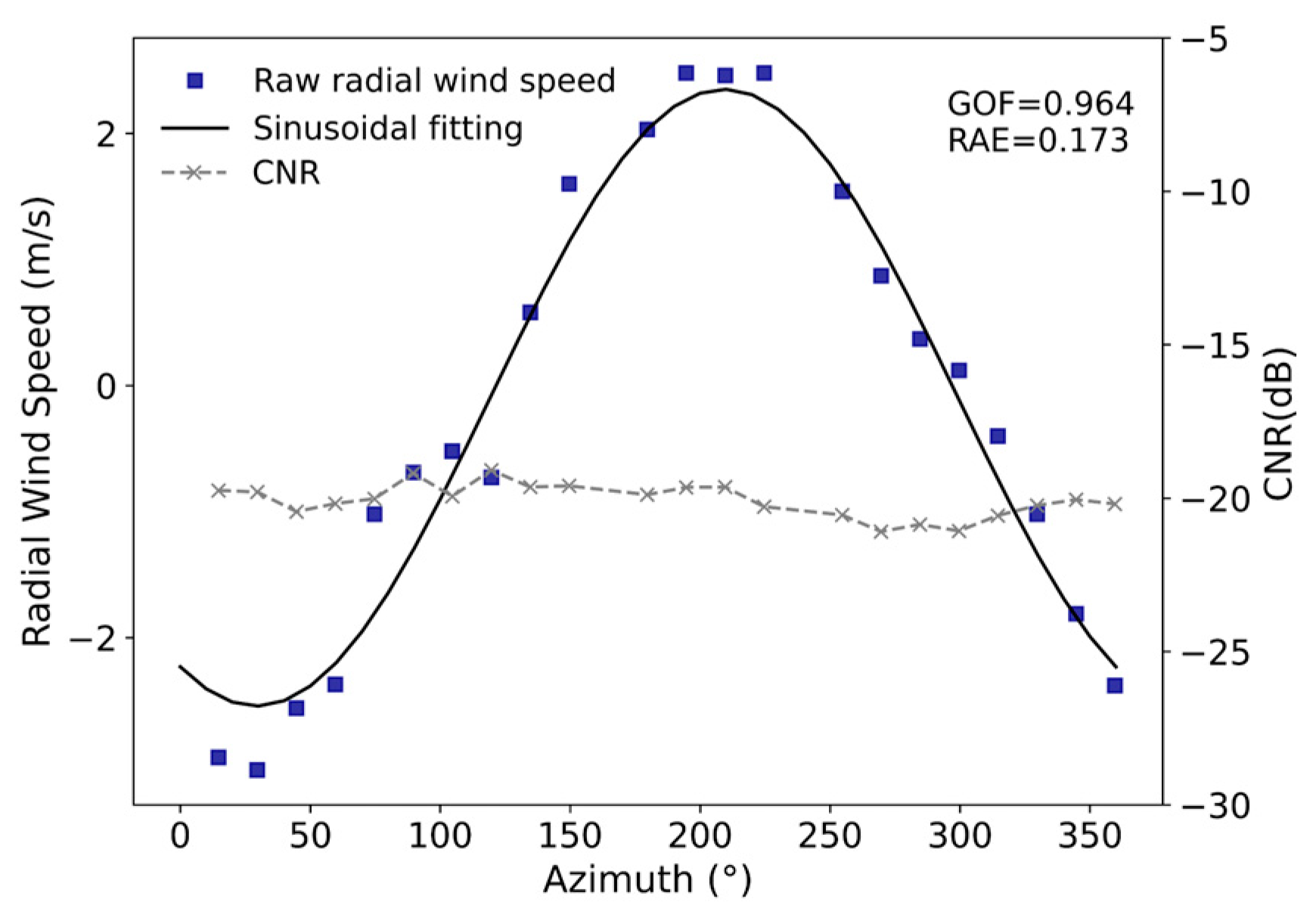
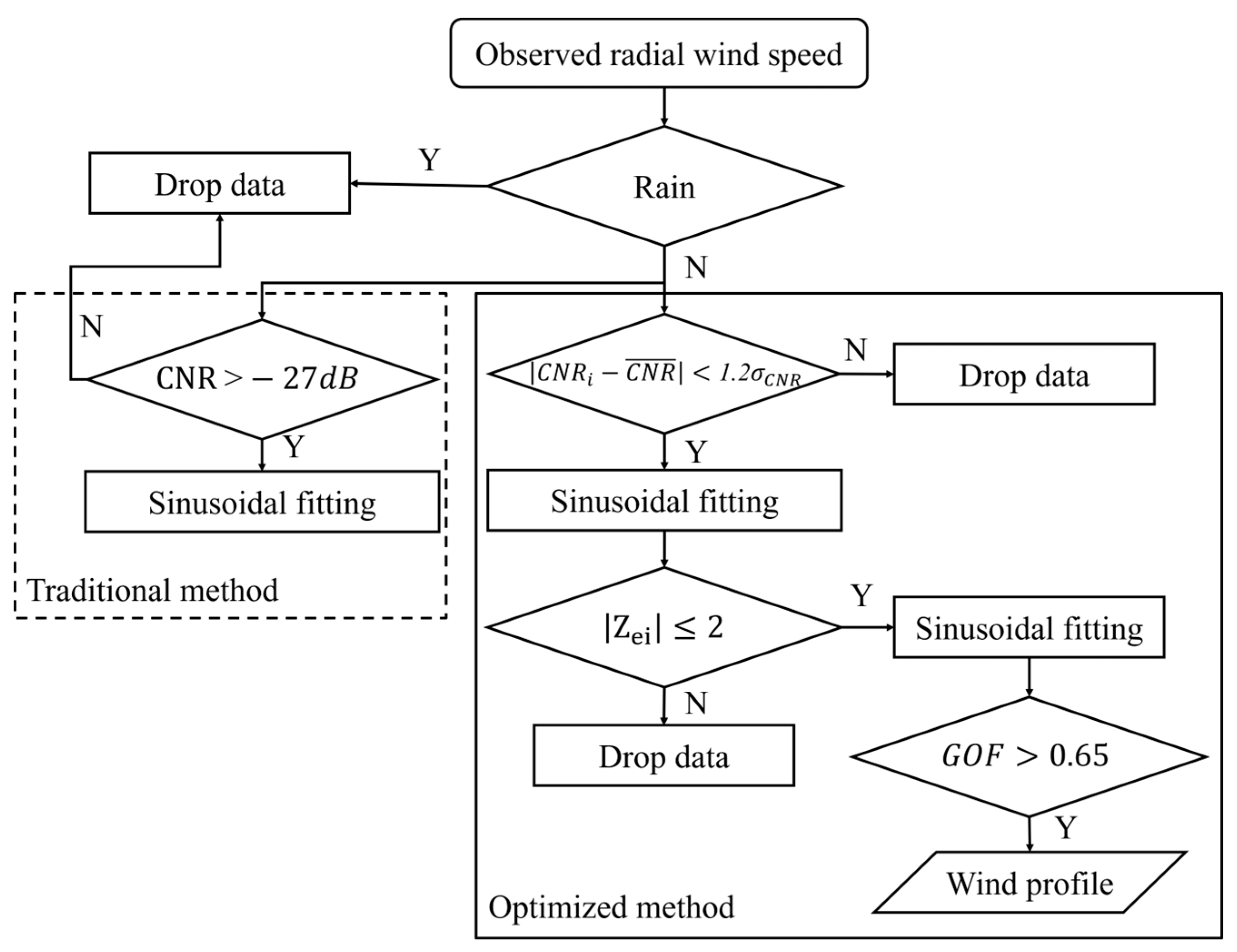
2.2. Inversion Method

In a horizontally homogeneous wind field, the variation of radial wind speed with azimuth for a VAD scan follows a sinusoidal curve [24] (refer to Figure 2). Thus, vertical profiles of horizontal wind vectors can be obtained by performing triangular transformation and sinusoidal fitting of radial wind speed with azimuth at each height [15]. The equations are as follows [24]:

$$V_{0i}=a+b·\cos \left({\theta }_i-{\theta }_{max}\right),$$

(1)

$$W_s=\frac{b}{\cos \phi },$$

(2)

$$W_d=\left\{\begin{array}{ll}{\theta }_{max}& ifb<0\\ {\theta }_{max}+\pi & ifb\ge 0\end{array}\right.,$$

(3)

where $V_{0i}$ is the radial wind speed (negative when coming to the Lidar) at i th direction (i = 1,… 24) (e.g., the squares in Figure 2), $a$ is the vertical shift of the sinusoidal fitting curve, which can be used to derive the vertical velocity, b is the amplitude of the sinusoidal fitting curve, ${\theta }_{max}$ is the phase shift (for the definition of $a$, $b$, and ${\theta }_{max}$; please refer to Figure 2a), $\theta$ is the azimuth, $\phi$ is the elevation angle, $W_s$ is the horizontal wind speed, and $W_d$ is the horizontal wind direction.

Before using the above method to derive the horizontal wind speed and direction, some preprocessing is required on the original radial wind speed data from the Lidar. The raw data recorded by Lidar not only include instantaneous radial wind speed but also the Confidence Index (CI), which indicates the reliability of the data. To eliminate unreliable data, data with CI = 0 are discarded. Since precipitation could significantly affect the performance of Lidar, data with precipitation greater than 1 mm are discarded. Considering the uncertainty of Lidar radial wind speed at low wind speeds, data with radial wind speeds less than 2 m/s are discarded [25].

In practice, the carrier-to-noise ratio (CNR) of some points in a given VAD will have outliers due to the influence of clouds or precipitation as well as the fact that some of the radial directions may be completely or partially obstructed by obstacles such as wind turbines or wind towers (as shown by the circles in Figure 2a). To control the quality of the Lidar radial wind speed data, previous studies usually set a threshold of CNR ≥ −27 dB or higher as a cutoff and exclude data below the threshold [26,27,28]. This traditional method is simple, but due to the influence of environmental factors such as noise levels, atmospheric conditions, and reflection characteristics of the target, just using CNR to screen data may potentially remove some high-quality data. Therefore, in this study, we remove outliers using the standard deviation of CNR (${\sigma }_{CNR})$ at each height in a full VAD scan. ${\sigma }_{CNR}$ is calculated using the following equations:

$$\overline{CNR}=\frac{1}{n}\sum _{i=1}^n{CNR}_i,$$

(4)

$${\sigma }_{CNR}=\sqrt{\frac{1}{n}\sum _{i=1}^n{\left({CNR}_i-\overline{CNR}\right)}^2},$$

(5)

where $\overline{CNR}$ is the average of CNR for all azimuths at a certain range gate, ${CNR}_i$ represents the CNR value at the i th direction, where i ranges from 1 to 24 (n = 24). In this study, data points with $\left|{CNR}_i-\overline{CNR}\right|$ >1.2${\sigma }_{CNR}$ are defined as outliers and removed.

As seen in Figure 2b, this method can effectively remove data points with abnormal CNR values (indicated by the green circles in Figure 2a), and improve the fitting. The Goodness of Fit (GOF) increases from 0.938 (Figure 2a) to 0.948 (Figure 2b), and the relative absolute error (RAE) decreases from 0.232 to 0.205. The GOF and RAE are calculated as follows:

$$\mathrm{G}\mathrm{O}\mathrm{F}=\frac{{\sum }_{i=1}^n{\left(V_{fit,i}-\overline{V_0}\right)}^2}{{\sum }_{i=1}^n{\left(V_{0i}-\overline{V_0}\right)}^2},$$

(6)

$$\mathrm{R}\mathrm{A}\mathrm{E}=\frac{\left|V_0-V_{fit}\right|}{V_0},$$

(7)

where $V_0$ is the observed radial wind speed, $V_{fit,i}$ is the corresponding fitted value, and $\overline{V_0}$ is the average of the observed radial wind speed.

If more than 10 data points are available in a full VAD at a certain range gate, then the wind direction and speed are sinusoidal fitted (the first fit) to derive the wind vectors at that range gate, otherwise the data are considered missing. In the calculation, we noticed that there are still some outliers (indicated by the red circle in Figure 2b) after using the ${\sigma }_{CNR}$ filter. In order to detect these outliers, the standardized residual ($Z_{\mathrm{e}}$) of the first fit is calculated. Since standard deviation (${\sigma }_{V_0}$) satisfies a normal distribution, $Z_{\mathrm{e}}$ also satisfies a normal distribution. If the $Z_{\mathrm{e}}$ of an azimuthal angle falls outside the range of (−2, 2), it is discarded at the 95% confidence interval. The standardized residual $Z_{\mathrm{e},\mathrm{i}}$ for each azimuth is calculated using the radial wind speed from the first fit ($V_{\mathrm{f}\mathrm{i}\mathrm{t}}$) and the observed radial wind speed ($V_0$) as follows.

$${\sigma }_{V_0}=\sqrt{\frac{1}{n}\sum _{i=1}^n{\left(V_{0i}-\overline{V_0}\right)}^2},$$

(8)

$$\overline{V_0}=\frac{1}{n}{\sum }_{i=1}^n{V}_{0i},$$

(9)

$$Z_{e,i}=\frac{V_{fit,i}-V_{0i}}{{\sigma }_{V_0}},$$

(10)

where ${\sigma }_{V_0}$ is the standard deviation of $V_0$, $V_{fit,i}$ is the fitted radial wind speed at the i th direction, $V_{0i}$ is the observed radial wind speed at the i th direction, $\overline{V_0}$ is the average of the observed radial wind speed at a certain range gate. Figure 3 shows the fitting result after removing outliers identified by the $Z_e$ filter. It can be seen that the point with large deviation has been removed. The GOF increases from 0.948 to 0.964 and the RAE decreases from 0.205 to 0.173.

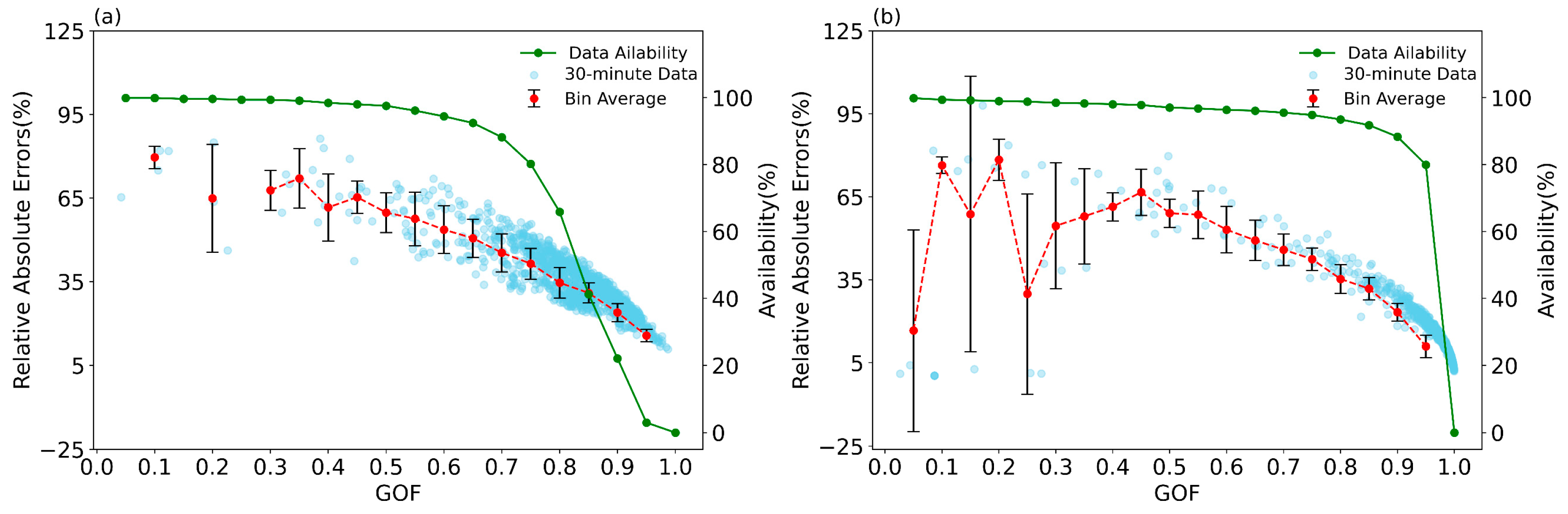
2.3. Optimize the Inversion Results

In this study, the fitting results are further evaluated and optimized using Goodness of Fit (GOF). GOF is generally used to characterize how well the fitted curves fit the observations [29] and is calculated using Equation (6). GOF ranges from 0 to 1, with values closer to 1 indicating a higher correlation between the fitted and the observed radial wind speed. Conversely, values nearing 0 indicate lower fitting quality. Hence, GOF serves as a reliable indicator for evaluating the accuracy of inversion results. Figure 4 shows the GOF across three fitting scenarios. Notably, when data points closely follow a sinusoidal curve and CNR values exceed −21 dB, the fitting results are excellent and GOF approaches 1 (Figure 4a, GOF = 0.989). Conversely, a GOF of 0.768 (Figure 4b) indicates a lower fitting quality, characterized by data points clustering near but not precisely on the fitting curve. In situations where data points are significantly scattered with considerable CNR fluctuations, the GOF drops substantially (Figure 4c, GOF = 0.565). These observations imply that lower GOF values, influenced by non-uniform wind fields, are associated with decreased precision in the derived wind speed.

Due to the absence of a standard threshold for Goodness-of-Fit (GOF) values, previous studies often rely on the proximity of GOF to 1 as an indicator of fitting quality [30]. In this study, a critical GOF value appropriate for the observational context of this research is identified by examining how GOF varies with the relative absolute error (RAE) of the fitted wind speed. RAE is primarily utilized to assess the accuracy of the fitting results [9], with better fitting results as it approaches zero. RAE is calculated using Equation (7).

Figure 5a,b illustrate the variation of RAEs as a function of the GOF values for 10 m at S1 and S3, respectively. As the GOF value increases, the corresponding amount of usable data decreases. Specifically, at S3, when GOF is below 0.65, the RAE is above 50%, when GOF is greater than 0.65, the usable data are less than 90%. Consequently, in this study, a GOF above 0.65 is adopted to optimize the final fitting results. Figure 6 depicts the data quality control process proposed in this study, along with the traditional method commonly referenced in the literature (delineated by dashed lines). The procedure initiates with the removal of rainfall-affected data, followed by the exclusion of data with anomalously high or low CNR values using $\left|{CNR}_i-\overline{CNR}\right|$ > 1.2${\sigma }_{CNR}$. An initial sinusoidal fitting is then conducted and the standardized residual ($Z_{e,i}$) of the results is calculated. Data points with $\left|Z_e\right|$ > 2 are excluded, before the second sinusoidal fitting. Finally, the horizontal wind speed and direction inversion outcomes with GOF above 0.65 are retained.

2.4. Statisitc Calculation

Due to the vector characteristic of wind direction, the numeric values of differences between the derived wind direction and that measured by the meteorological tower may not reflect the actual differences when the differences are greater than 180°. This limitation is addressed by modifying the derived wind direction following [31,32] when evaluating the derived wind direction, i.e.,

$${WD}_{\mathrm{l}\mathrm{i}\mathrm{d}\mathrm{a}\mathrm{r}}=\left\{\begin{array}{l}{WD}_{\mathrm{l}\mathrm{i}\mathrm{d}\mathrm{a}\mathrm{r}}if\left|{WD}_{\mathrm{t}\mathrm{o}\mathrm{w}\mathrm{e}\mathrm{r}}-{WD}_{\mathrm{l}\mathrm{i}\mathrm{d}\mathrm{a}\mathrm{r}}\right|\le 180\\ {360-WD}_{\mathrm{l}\mathrm{i}\mathrm{d}\mathrm{a}\mathrm{r}}if{WD}_{\mathrm{t}\mathrm{o}\mathrm{w}\mathrm{e}\mathrm{r}}-{WD}_{\mathrm{l}\mathrm{i}\mathrm{d}\mathrm{a}\mathrm{r}}<-180\\ {360+WD}_{\mathrm{l}\mathrm{i}\mathrm{d}\mathrm{a}\mathrm{r}}if{WD}_{\mathrm{t}\mathrm{o}\mathrm{w}\mathrm{e}\mathrm{r}}-{WD}_{\mathrm{l}\mathrm{i}\mathrm{d}\mathrm{a}\mathrm{r}}>180\end{array}\right.,$$

(11)

After this step, the differences in wind direction are within the range of [−180°, 180°]. This resolves the impact of the periodic change in wind direction on the results of regression analysis and statistic calculations. The mean absolute error (MAE), root mean square error (RMSE), and coefficient of determination (R²) are used to evaluate the quality of derived wind. They are defined as follows:

$$\mathrm{MAE}=\frac{1}{t}{\sum }_{i=1}^t\left|{WS}_{\mathrm{t}\mathrm{o}\mathrm{w}\mathrm{e}\mathrm{r},\mathrm{i}}-{WS}_{\mathrm{l}\mathrm{i}\mathrm{d}\mathrm{a}\mathrm{r},\mathrm{i}}\right|,$$

(12)

$$\mathrm{RMSE}=\sqrt{\frac{1}{m}{\sum }_{i=1}^m{\left({WS}_{\mathrm{l}\mathrm{i}\mathrm{d}\mathrm{a}\mathrm{r},\mathrm{i}}-{WS}_{\mathrm{t}\mathrm{o}\mathrm{w}\mathrm{e}\mathrm{r},\mathrm{i}}\right)}^2},$$

(13)

$${\mathrm{R}}^2=1-\frac{{\sum }_{i=1}^m{\left({WS}_{\mathrm{t}\mathrm{o}\mathrm{w}\mathrm{e}\mathrm{r},\mathrm{i}}-{WS}_{\mathrm{l}\mathrm{i}\mathrm{d}\mathrm{a}\mathrm{r},\mathrm{i}}\right)}^2}{{\sum }_{i=1}^m{\left({WS}_{\mathrm{t}\mathrm{o}\mathrm{w}\mathrm{e}\mathrm{r},\mathrm{i}}-\overline{{WS}_{\mathrm{t}\mathrm{o}\mathrm{w}\mathrm{e}\mathrm{r},\mathrm{i}}}\right)}^2},$$

(14)

where m is the number of paired samples, ${WS}_{\mathrm{t}\mathrm{o}\mathrm{w}\mathrm{e}\mathrm{r}}$ is the wind speed measured by the meteorological tower, ${WS}_{\mathrm{l}\mathrm{i}\mathrm{d}\mathrm{a}\mathrm{r}}$ is the derived wind speed using the optimized or the traditional method.

2.5. Kolmogorov–Smirnov (K-S) Test

The Kolmogorov–Smirnov (K-S) test, a significance testing method, leverages sample data to determine if the population from which the sample was taken differs significantly from a theoretical distribution. This technique utilizes F(x) to denote the theoretical cumulative probability of each sample observation against the theoretical distribution, and S(x) for the actual cumulative probabilities. The test’s statistic, D, is derived as the maximum absolute difference between F(x) and S(x): D = $\mathrm{m}\mathrm{a}\mathrm{x}\left|F\left(x\right)-S\left(x\right)\right|$.

Under the null hypothesis, D follows the Kolmogorov distribution. The test calculates a corresponding p-value; if p falls below the significance level α, the null hypothesis is rejected, suggesting a significant deviation between the sample’s population and the theoretical distribution. Conversely, a higher p-value indicates no significant difference. In this study, the K-S test was applied to compare the inversion results from an optimized method against those from a traditional approach, assessing significant enhancements in the optimized method’s outcomes.

In this study, an optimized method is used to quality control the raw radial wind data from scanning Doppler Lidar and optimize the inversion results under different complexities of wind field environments (inside and upwind of a wind farm). The proposed method improves the quality of vertical wind profiles from near the ground level to the heights impacted by wind turbine blades. Such kind of information can be used for wind power prediction as well as studies of the climatic and environmental effects of wind farm operations. Due to the lack of in situ boundary layer wind profile data, the derived wind speed and wind direction are validated using observations from 10 m and 70 m wind tower data and DBS reconstructed data.

3. Results

3.1. Wind Condition during the Experiment

During the study period, the 70 m tower within the wind farm registered an average monthly wind speed of 7.2 m/s at 70 m above the ground level (AGL) with a peak wind speed of 24.2 m/s. The majority of wind speeds ranged from 2 to 10 m/s (Figure 7a). The dominant wind directions were northwest (NW) and northeast (NE), with directions spanning from 0° to 90° and 270° to 360° comprising over 60% of the total observations (Figure 7b).

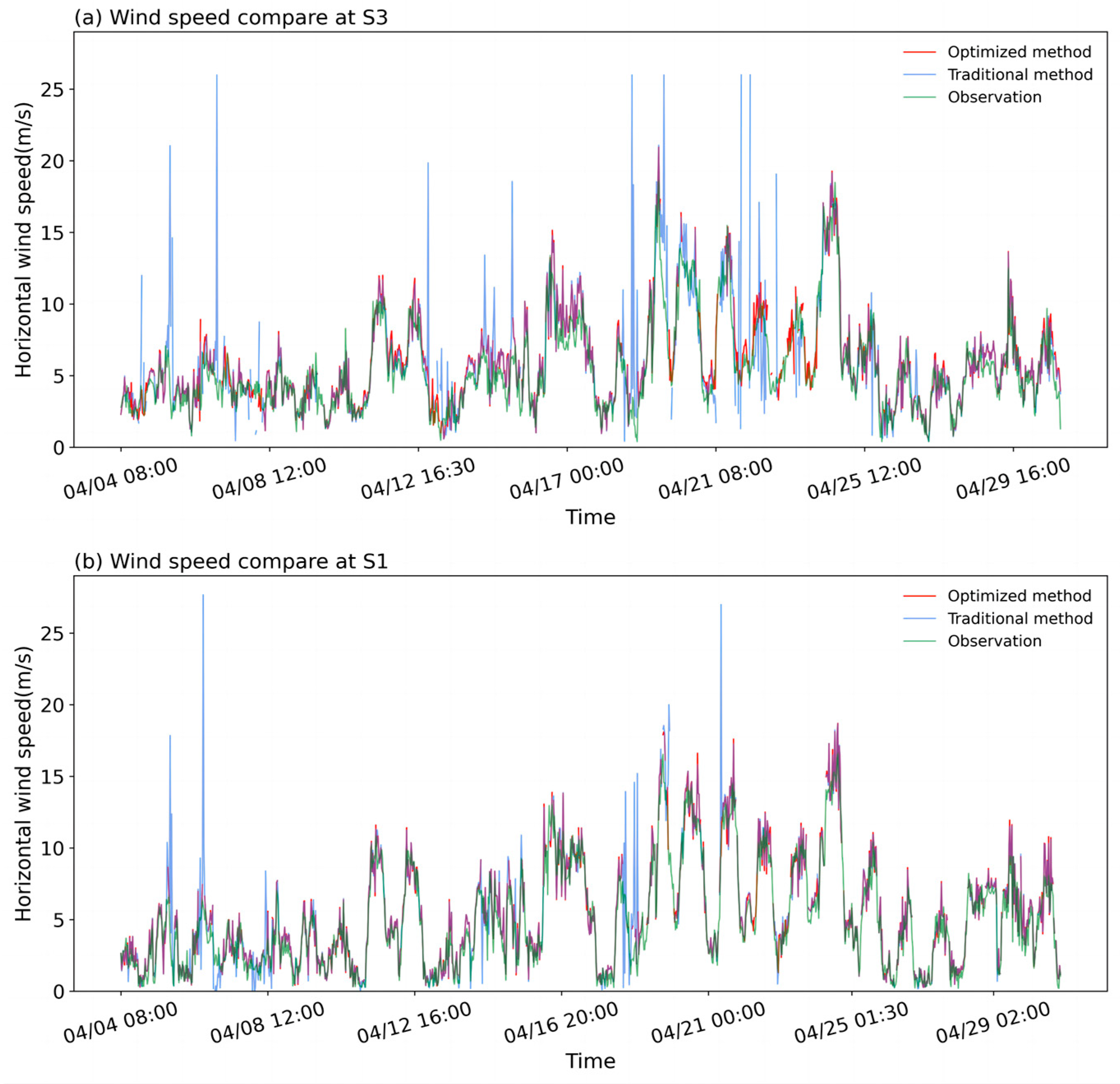
3.2. Validation of the Derived Wind

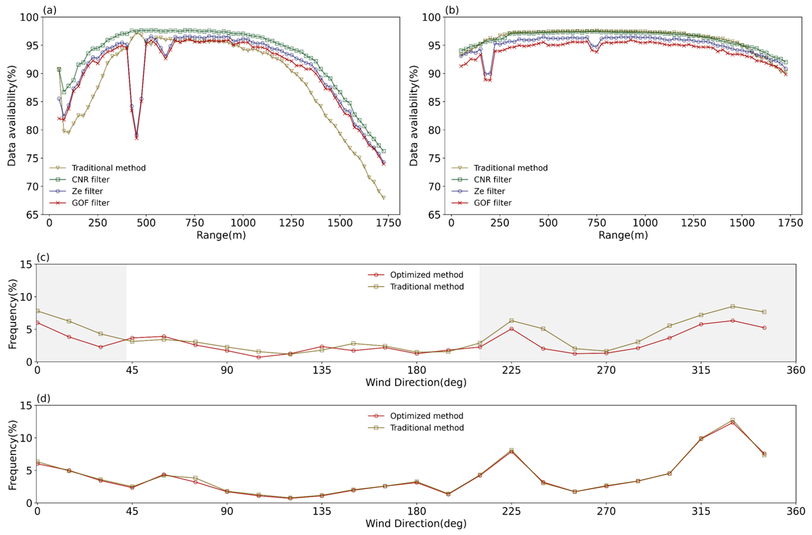
3.2.1. Different Quality Control Methods

Figure 8 shows the comparison between the wind speeds derived using the optimized method (${WS}_{\mathrm{l}\mathrm{i}\mathrm{d}\mathrm{a}\mathrm{r}}$) and those measured by meteorological tower (${WS}_{\mathrm{t}\mathrm{o}\mathrm{w}\mathrm{e}\mathrm{r}}$). The wind speeds derived at two heights (10 m and 70 m) using the radial wind speed from VAD scans at two elevation angles (10° and 30°) at two distinct sites, i.e., within the wind farm (S3) and upwind of the wind farm (S1), are shown. Wind speed derived from the optimized method are in good agreement with those measured by the meteorological tower, with a linear regression slope between 0.991 and 1.069, and a coefficient of determination exceeding 0.932. The volume of usable data is greater than 75% (the total data volume used for comparison during the study period is 1277 pairs).

Table 1. Statistical comparison between Lidar-derived and meteorological tower-measured wind speed. Bold and plain numbers are for the optimized and the traditional methods, respectively.

Elevation Angle	Site/Height	MAE (m/s)	RMSE (m/s)	R2	Significance
10°	S1/10 m	0.748	1.029	0.965
		0.859	1.433	0.934
	S3/10 m	0.927	1.239	0.932	*
		1.231	2.116	0.826
	S3/70 m	0.771	1.102	0.958	*
		1.023	1.470	0.926
30°	S3/70 m	0.903	1.210	0.954	**
		1.326	2.253	0.838

** The difference passed the Kolmogorov–Smirnov test with a confidence level of $\alpha$ = 0.01. * The difference passed the Kolmogorov–Smirnov test with a confidence level of $\alpha$ = 0.05.

gives the statistical results from the comparison of wind speeds derived using the optimized and traditional methods at different observation sites and heights against those measured by the meteorological tower. The significance of the difference between the results from the traditional and the optimized methods are tested using the Kolmogorov–Smirnov test, and the results are indicated in the last column in Table 1. Within the wind farm (S3), the optimized method significantly enhances the accuracy of the derived wind speed at 10 m and 70 m (significant at $\alpha$ = 0.05) for the 10-degree elevation angle, and at 70 m (significant at $\alpha$ = 0.01) for the 30-degree elevation angle. The results from the optimized method exhibit better R² values compared to those from the traditional method, particularly within the wind farm (S3) where the wind field is more complex. The statistics of our inversion results are better than similar studies by Wang (R² = 0.956 at h = 74 m) using combined filtering [33], and by Hauke [34] using dynamic data filtering (R² = 0.85 at h = 41.5 m) and static standard deviation filtering (R² = 0.83 at h = 41.5 m). The optimized method also gives lower MAE and RMSE. The above results indicate that the optimized method is effective for deriving wind speed in complex wind environments, for example, within wind farms.

Similar to the wind speed analysis, Figure 9 presents the scatter plots that compare the wind directions derived using VAD scans (${WD}_{\mathrm{l}\mathrm{i}\mathrm{d}\mathrm{a}\mathrm{r}}$) with different elevation angles (10° and 30°) against those from tower measurements (${WD}_{\mathrm{t}\mathrm{o}\mathrm{w}\mathrm{e}\mathrm{r}}$). Results from the optimized and the traditional methods at different heights (10 m and 70 m) and different sites (S1 and S3) are compared.

Table 2. Comparison between Lidar-derived and meteorological tower measured wind directions. Bold and plain numbers are for the optimized and the traditional methods, respectively.

Elevation Angle	Site/Height	MAE (°)	RMSE (°)	R2	Significance
10°	S1/10 m	11.323	19.168	0.987
		13.744	25.392	0.977
	S3/10 m	14.715	19.242	0.992	*
		18.272	27.453	0.978
	S3/70 m	13.714	16.255	0.995	*
		16.075	20.840	0.983
30°	S3/70 m	13.731	17.626	0.993	*
		18.419	26.891	0.978

* The difference passed the Kolmogorov–Smirnov test with a confidence level of $\alpha$ = 0.05.

shows the statistical results. Similarly, the wind direction obtained by both the traditional and the optimized methods show good correlations with observations from the meteorological tower. At 70 m, the derived wind directions using optimized methods are better than those in a similar study carried out by Lang et al. (R² = 0.947 at h = 78 m) [22]. The optimized method improves the wind direction inversion when compared to the traditional method, as evidenced by the significant increase in the coefficient of determination. In the subsequent sections, we will focus our analysis on the effects of the proposed optimized method on wind speed inversions.

Figure 10 illustrates a comparison between the wind speed derived using the traditional and the optimized methods at S1 (upstream of the wind farm) and S3 (inside the wind farm) with the 10° elevation angle VADs in every half hour and those measured by the meteorological tower. Compared to the optimized method, the results from the traditional method have some abnormally large or small values relative to the observations from the meteorological tower. The consistency between the optimized method and the meteorological tower observations is better, especially within the wind farm (Figure 10a).

3.2.2. Different Weather Conditions

Previous studies have demonstrated that Lidar can not only detect signals scattered by aerosols but also capture background signals. Daytime background signals, primarily composed of direct or scattered light, are more intense than nighttime signals, predominantly originating from the moon and artificial light sources [35]. Therefore, considering the influence of background signals is essential when analyzing factors that affect the derived wind speed and direction. Additionally, atmospheric hydrometeors, such as clouds and raindrops, cause signal attenuation through particulate scattering, leading to a decrease in CNR. In the following, the performances of the optimized and traditional methods are compared under clear and cloudy conditions and during the day and night.

The clear-sky index (CSI) has been used in previous studies to distinguish clear skies from cloudy conditions [36,37,38]. Utrillas et al. [39] compared CSI with ceilometer readings and noted a high correlation. In this study, the longwave downward radiation (LDR) data from the four-component radiometer at S3 and air temperature and humidity data from the meteorological tower are used to calculate the CSI following Dürr and Philipona [34]:

$$CSI=\frac{{\in }_A}{{\in }_{AC}},$$

(15)

$${\in }_A=\frac{LDR}{{\sigma }_S{T}^4},$$

(16)

$${\in }_{AC}={\in }_{AD}+\left(k+2{\sigma }_S\right){\left(\frac{e}{T}\right)}^{1/8},$$

(17)

where ${\sigma }_S$ is the Stephen—Boltzmann constant, T is the air temperature (K), ${\in }_A$ is the apparent emittance of the sky, ${\in }_{AC}$ is the empirical apparent cloud-free emittance, ${\in }_{AD}$ represents the altitude-dependent clear-sky emittance of a completely dry atmosphere. In Equation (17), e is the water vapor pressure (Pa), and k is a position coefficient of determination. The water vapor pressure e is calculated from the relative humidity using the following equations:

$$e=\frac{RH}{100}{e}_s,$$

(18)

$$e_s=6.1121exp\left(\frac{17.502t}{t+240.97}\right),$$

(19)

where RH is the relative humidity (%), $e_s$ is the saturated water vapor pressure (hPa), t is the air temperature (°C). The coefficient k is location-dependent and determined by fitting ${\in }_A$ and e/T (Figure 11) using Equation (17) [33].

A clear-sky index exceeding 1 suggests cloud presence, whereas a CSI of 1 or below indicates a cloud-free condition. During the study period, there are a total of 1277 half-hourly observations, of which 375 are cloudy (212 of which are daytime observations and 163 of which are nighttime observations) and 902 are clear (431 of which are daytime and 471 of which are nighttime observations).

Table 3. Comparison of day and night wind speed from Lidar and tower observations under cloudy and clear-sky conditions at S3. Bold and plain numbers are for the optimized and the traditional methods, respectively.

Condition		Number	R2	RMSE (m/s)	MAE (m/s)	Significance
Cloudy period	Daytime	168	0.925	1.734	1.358	*
		197	0.813	2.646	1.699
	Nighttime	118	0.932	1.275	0.978
		134	0.905	1.585	1.130
Clear-sky period	Daytime	381	0.927	1.294	0.987	*
		411	0.845	2.031	1.222
	Nighttime	433	0.918	0.909	0.699
		388	0.889	1.096	0.765

* The difference passed the Kolmogorov–Smirnov test with a confidence level of α = 0.05.

shows the statistical results for the comparison of the derived wind speeds (using the optimized and the traditional methods) with those measured by the meteorological tower under cloudy and clear sky conditions. Despite the reduced data availability, the optimized method outperforms the traditional method in the coefficient of determination (R²), root mean square error (RMSE), and mean absolute error (MAE). Under cloudy conditions, the R² for the optimized method (0.925 during the day (07: 00–18: 30) and 0.932 during the night (19: 00–06: 30)) exceed those of the traditional method (0.813 during the day and 0.905 during the night). Thus, the wind speed derived using the optimized method is more accurate. In addition, the optimized method consistently gives lower RMSE and MAE than the traditional method, especially under cloudy conditions. On clear nights, the traditional CNR threshold method may exclude some high-quality data points, leading to a decrease in data availability and lower R². In contrast, the optimized method not only retains more original data, with an increase of 9.5%, but also significantly improves the inversion accuracy.

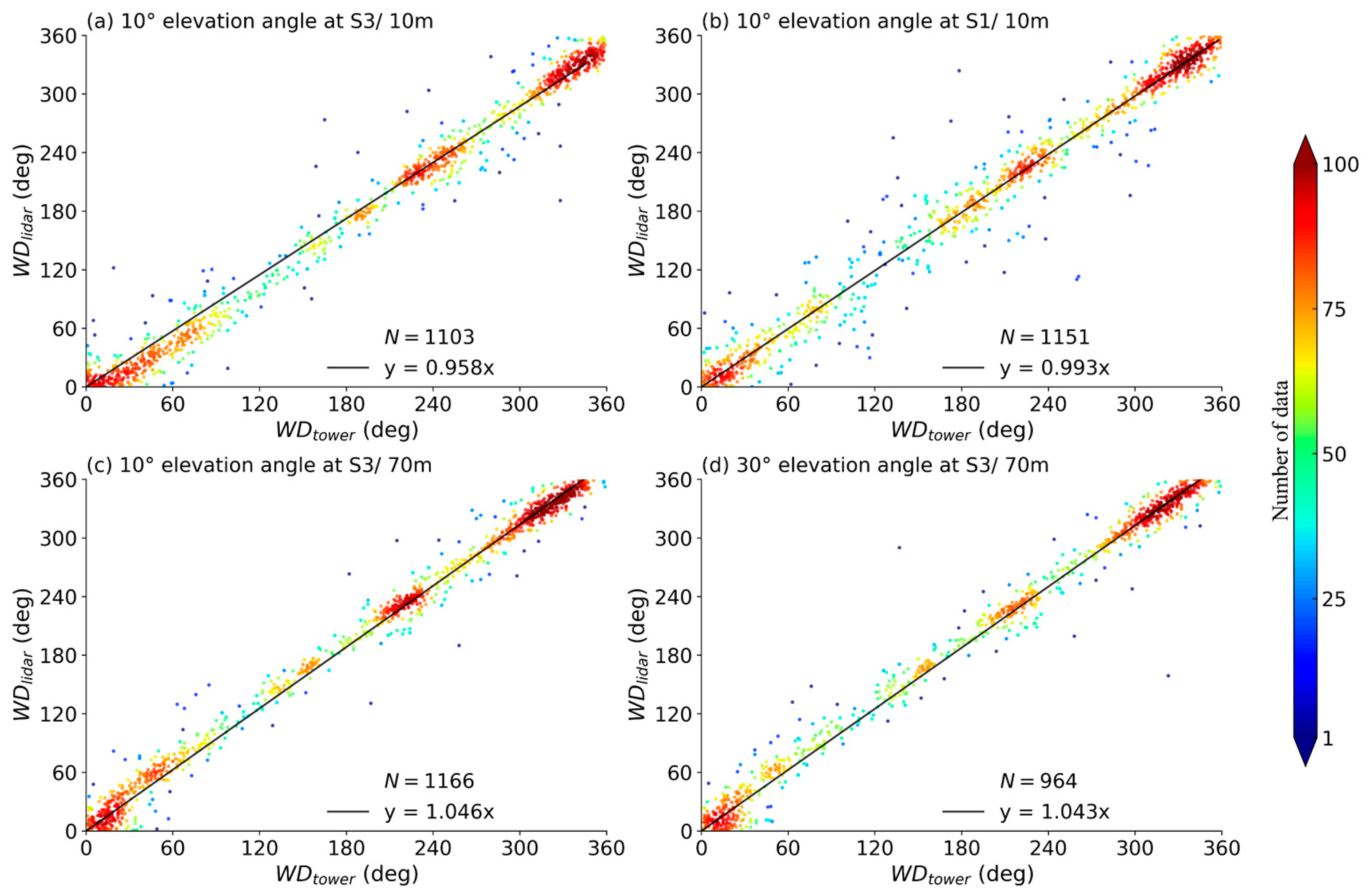
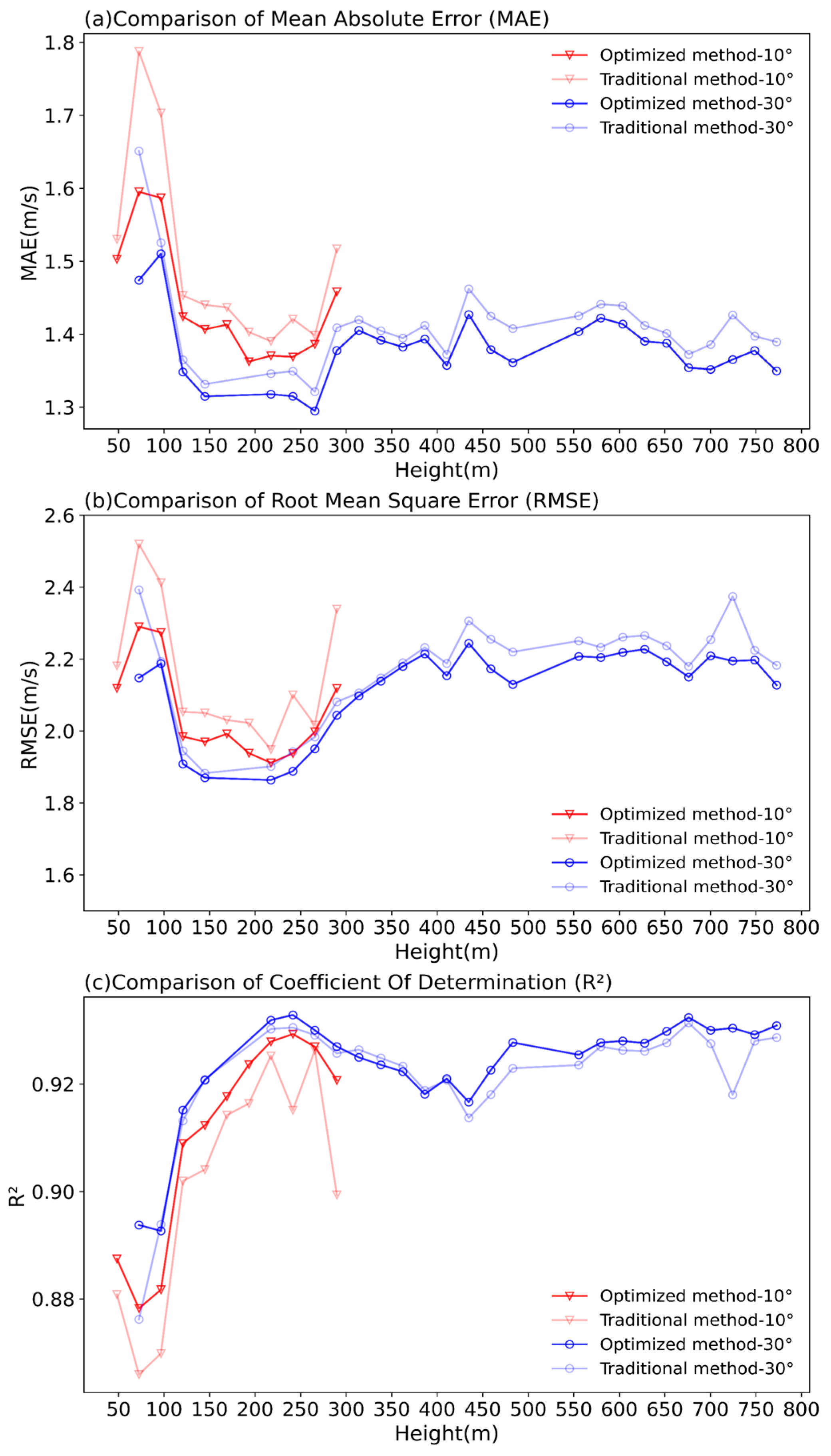
3.2.3. Validation of Wind Profiles

The Doppler beam-swinging (DBS) scanning mode, emitting five beams towards the east, south, west, north, and vertical in sequence at a 75° elevation angle, acquires radial wind speeds in five directions: V_E, V_S, V_W, V_N, and ω. When the Lidars are operating in the DBS mode, they can provide files containing reconstructed wind, including the meridional (u) and the zonal (v) wind components, derived using a method similar to Lundquist et al. [21]. These data are used to further evaluate the performance of the optimized method, with a purpose for its potential to extend the height with acceptable accuracy, as it is known that the assumption of a horizontally homogeneous atmosphere used in the inversion method is increasingly difficult to satisfy with the increasing detection height, and the accuracy of inversion results might decrease, particularly for low-elevation-angle VAD scans. A wind profile spanning 8–800 m can be obtained by the inversions from VAD scans with 10° (8–300 m) and 30° elevation angles (25–800 m). Here, the wind profiles derived from the optimized method are evaluated using the wind profiles obtained from DBS scanning as a benchmark.

Figure 12 shows the MAE (Figure 12a), RMSE (Figure 12b) and R² (Figure 12c) between the wind speed derived from the optimized/the traditional methods and those from DBS reconstruction at S3 from VADs with both elevations. It can be observed that the accuracy of the wind speed derived from the optimized method is superior to that from the traditional method in terms of all the three statistics. Notably, at certain heights, such as near the hub height of 78 m, the error from the traditional method shows abnormally high values (pink line and light blue lines in Figure 12), while this error is significantly reduced after using the optimized method (red and blue lines in Figure 12), indicating an improvement in the performance of the optimized method. In addition, the optimized method has the potential to extend the height with acceptable wind accuracy, especially for low-elevation-angle scanning. For example, in the last gate of the 10° elevation VAD scan, the statistics of the wind speed derived using the optimized method were significantly improved. Generally, the results obtained using a 30° elevation VAD scan are better than those obtained using a 10° elevation VAD scan. The above analysis indicates that the wind speed derived from the optimized method is more consistent with the wind speed reconstructed by DBS. Therefore, the optimized method can be used to derive wind profiles from below the minimum range of a vertically operating scanning Doppler Lidar to above the height affected by wind turbines.

4. Discussion

The optimized quality control method proposed in this study will gradually reduce the amount of valid data as the control criterion becomes progressively stricter. Previous studies have shown that data availability can affect the climatic characteristics of the resulting wind field in a study area [40,41]. For example, these studies shows that when the quality control process is more stringent, it will reduce the amount of usable data, which can lead to an overestimation of wind speed distribution. Therefore, it is necessary to study the impact of the optimized method on the amount of usable data. In Figure 13a,b, the amount of valid data at S3 and S1, after each step of control using the traditional and optimized methods are given, with the horizontal axis indicating the radial distance for the 10° elevation angle VAD. Within the wind farm (S3) (Figure 13a), the amount of available data (data availability) after ${\sigma }_{CNR}$ filtering is higher than the traditional method at all heights. After $Z_e$ filtering and GOF optimization, the amount of available data is higher than the traditional method at radial distances below 400 m and above 1750 m, while it is similar to that of the traditional method in the range of 400–1750 m. It is noted that at the radial distance of 450 m, the amount of available data is significantly lower than the traditional method, which is attributable to the presence of wind turbines in the azimuth range of 225°–15° at S3, with the vertical height corresponding to this radial distance close to the hub height of the wind turbines. Upwind of the wind farm (S1) (Figure 13b), the data availability after ${\sigma }_{CNR}$ filtering is similar to the traditional method but slightly less than the traditional method after $Z_e$ filtering and GOF optimization (about 5%). The above analysis suggests that the quality control of Lidar radial wind speed data and the optimized processing procedure proposed in this study can retain more valid data in complex wind field environments, such as inside a wind farm. Figure 13c,d present the ratio of the available data in each 15° wind direction interval to the total data at S3 and S1, using the traditional and the optimized methods, respectively. At S1, the data availability of the traditional method and the optimized method are comparable in all azimuths (Figure 13d), while the data availability of the optimized method is lower than that of the traditional method in the range of 210°–42° at S3 (Figure 13c) but still exceeds 75% (Figure 13a), which indicates that the optimized method can effectively filter out the data affected by wind turbines. Overall, the optimized method not only improves the accuracy of wind speed inversion but also maintains a larger amount of valid data than the traditional method, particularly in complex wind field environments.

5. Conclusions

In a horizontally homogeneous wind field, the vertical profiles of the horizontal wind vector can be obtained by sinusoidal fitting the radial wind speeds and azimuth angle in a VAD at each range gate. In this study, based on the radial wind speed data acquired by a scanning Doppler Lidar, an optimized method for raw radial wind speed data quality control and inversion result optimization is proposed (Figure 6). The method applies the ${\sigma }_{CNR}$ filter to exclude data with exceptionally high or low CNR values, followed by an initial sinusoidal fitting. Then, data points with standardized residuals ($\left|{\mathrm{Z}}_e\right|$) exceeding 2 are dropped before a second sinusoidal fitting. Finally, only the inversion results with GOF above 0.65 are retained. A comparison between the derived wind speed/wind direction from the optimized method and those from conventional observations underscore the advantages of the proposed method. A full vertical wind profile from near ground level to the height impacted by wind turbine blades can be obtained using the optimized method. The coefficient of determination (R²) between the wind speeds derived using the optimized method and those measured by the meteorological tower are higher compared to that of the traditional method (such as removing data with CNR < −27 dB), and the root mean square error (RMSE) and mean absolute error (MAE) are lower than those of the traditional method. Specifically, for a 10 m wind speed, R² is improved from 0.826 to 0.932, and the MAE is reduced from 1.231 to 0.927; for a 10 m wind direction, R² is improved from 0.978 to 0.992, and the RMSE is decreased from 27.453 to 19.242, especially within the wind farm where the wind conditions are more complex.

In this study, we improved the wind speed/wind direction inversion results by firstly removing outliers in the raw radial wind speed using filters such as ${\sigma }_{CNR}$ and ${\mathrm{Z}}_e$, then optimizing the derived wind speed/wind direction using the GOF threshold. The error of this method is notably lower than that of the traditional method, particularly during nighttime. Furthermore, this method significantly increases the amount of usable data, especially on clear nights. The comparison of data availability between the traditional and optimized methods reveals that the optimized method proposed not only improves the accuracy of wind speed inversion but also increases the amount of usable data, especially in complex wind field environments.

Low-elevation-angle VAD scanning has been proven to be a useful practice to obtain wind profiles below the minimum range of a vertically operating scanning Doppler Lidar. The optimized data quality control and inversion technique developed in this study is effective for obtaining wind profiles from near the ground to the height affected by wind turbines. This capability is vital for the in-depth analysis of the influence of wind turbine operation on a wind field and for the study of low-level jets, turbulence, and wind characteristics in wind farms and beyond. Future research should focus on validating and refining this method using data from diverse climatic conditions and terrains. Moreover, integrating different scanning strategies to determine an optimal balance between data quality and data availability is essential.

References

1. Balat, M. A Review of Modern Wind Turbine Technology. Energy Sources Part A Recovery Util. Environ. Eff. 2009, 31, 1561–1572. [Google Scholar] [CrossRef]
2. Roga, S.; Bardhan, S.; Kumar, Y.; Dubey, S.K. Recent technology and challenges of wind energy generation: A review. Sustain. Energy Technol. Assess 2022, 52, 102239. [Google Scholar] [CrossRef]
3. Politis, E.S.; Prospathopoulos, J.; Cabezon, D.; Hansen, K.S.; Chaviaropoulos, P.K.; Barthelmie, R.J. Modeling wake effects in large wind farms in complex terrain: The problem, the methods and the issues. Wind Energy 2012, 15, 161–182. [Google Scholar] [CrossRef]
4. Barthelmie, R.J.; Hansen, K.; Frandsen, S.T.; Rathmann, O.; Schepers, J.G.; Schlez, W.; Phillips, J.; Rados, K.; Zervos, A.; Politis, E.S.; et al. Modelling and measuring flow and wind turbine wakes in large wind farms offshore. Wind Energy 2009, 12, 431–444. [Google Scholar] [CrossRef]
5. Smith, C.M.; Barthelmie, R.J.; Pryor, S.C. In situ observations of the influence of a large onshore wind farm on near-surface temperature, turbulence intensity and wind speed profiles. Environ. Res. Lett. 2013, 8, 1–9. [Google Scholar] [CrossRef]
6. Li, Q.; Gulgina, H.; Kong, T.; Liu, W.; Gong, X.; Hu, Y.; Liu, Z. Quality Control and Effect Evaluation of Wind Tower Data in China. J. Desert Oasis Meteorol. 2024, 18, 141–148. [Google Scholar]
7. Gryning, S.; Batchvarova, E.; Brümmer, B.; Jørgensen, H.; Larsen, S. On the extension of the wind profile over homogeneous terrain beyond the surface boundary layer. Bound. -Layer Meteorol. 2007, 124, 251–268. [Google Scholar] [CrossRef]
8. Cao, J.; Xue, W.; Mao, R.; Xin, D. Wind power in forested regions: Power law extrapolation vs. lidar observation. J. Wind. Eng. Ind. Aerodyn. J. Int. Assoc. Wind. Eng. 2023, 232, 105281. [Google Scholar] [CrossRef]
9. Shimada, S.; Goit, J.P.; Ohsawa, T.; Kogaki, T.; Nakamura, S. Coastal Wind Measurements Using a Single Scanning Lidar. Remote Sens. 2020, 12, 1347. [Google Scholar] [CrossRef]
10. Theuer, F.; van Dooren, M.F.; von Bremen, L.; Kühn, M. Lidar-based minute-scale offshore wind speed forecasts analysed under different atmospheric conditions. Meteorol. Z. 2022, 31, 13–29. [Google Scholar] [CrossRef]
11. Emeis, S.; Harris, M.; Banta, R.M. Boundary-layer anemometry by optical remote sensing for wind energy applications. Meteorol. Z. 2007, 16, 337–347. [Google Scholar] [CrossRef] [PubMed]
12. Bianco, L.; Wilczak, J.M.; White, A.B. Convective Boundary Layer Depth Estimation from Wind Profilers Statistical Comparison between an Automated Algorithm and Expert Estimations. J. Atmos. Ocean. Technol. 2008, 25, 1397–1413. [Google Scholar] [CrossRef]
13. Srinivasulu, P.; Yasodha, P.; Kamaraj, P.; Rao, T.N.; Jayaraman, A.; Reddy, S.N.; Satyanarayana, S. 1280-MHz Active Array Radar Wind Profiler for Lower Atmosphere System Description and Data Validation. J. Atmos. Ocean. Technol. 2012, 29, 1455–1470. [Google Scholar] [CrossRef]
14. Vakkari, V.; O’Connor, E.J.; Nisantzi, A.; Mamouri, R.E.; Hadjimitsis, D.G. Low-level mixing height detection in coastal locations with a scanning Doppler lidar. Atmos. Meas. Tech. 2015, 8, 1875–1885. [Google Scholar] [CrossRef]
15. Browning, K.A.; Wexler, R. The determination of kinematic properties of a wind field using Doppler radar. J. Appl. Meteorol. 1968, 7, 105–113. [Google Scholar] [CrossRef]
16. Gao, H.; Shen, C.; Zhou, Y.; Wang, X.; Chan, P.; Hon, K.; Zhou, D.; Li, J. A Spatio-Temporal Neural Network for Fine-Scale Wind Field Nowcasting Based on Lidar Observation. IEEE J. Sel. Top. Appl. Earth Observ. Remote Sens. 2022, 15, 5596–5606. [Google Scholar] [CrossRef]
17. Baidar, S.; Wagner, T.J.; Turner, D.D.; Brewer, W.A. Using optimal estimation to retrieve winds from velocity-azimuth display (VAD) scans by a Doppler lidar. Atmos. Meas. Tech. 2023, 16, 3715–3726. [Google Scholar] [CrossRef]
18. Dong, D.; Yang, S.; Weng, N.; Zhang, G.; Huang, J. Analysis of Observation Performance of a Mobile Coherent Doppler Wind Lidar Using DBS Scanning Mode. J. Phys. Conf. Ser. 2021, 1739, 12048. [Google Scholar] [CrossRef]
19. Smith, D.A.; Harris, M.; Coffey, A.S.; Mikkelsen, T.; Jørgensen, H.E.; Mann, J.; Danielian, R. Wind lidar evaluation at the Danish wind test site in Høvsøre. Wind Energy 2006, 9, 87–93. [Google Scholar] [CrossRef]
20. Päschke, E.; Leinweber, R.; Lehmann, V. An assessment of the performance of a 1.5 μm Doppler lidar for operational vertical wind profiling based on a 1-year trial. Atmos. Meas. Tech. 2015, 8, 2251–2266. [Google Scholar] [CrossRef]
21. Lundquist, J.K.; Churchfield, M.J.; Lee, S.; Clifton, A. Quantifying error of lidar and sodar Doppler beam swinging measurements of wind turbine wakes using computational fluid dynamics. Atmos. Meas. Tech. 2015, 8, 907–920. [Google Scholar] [CrossRef]
22. Lang, S.; McKeogh, E. LIDAR and SODAR Measurements of Wind Speed and Direction in Upland Terrain for Wind Energy Purposes. Remote Sens. 2011, 3, 1871–1901. [Google Scholar] [CrossRef]
23. Xia, X. Effects of Wind Farms on Atmospheric Boundary Layer Meteorological Elements and Turbulent Fluxes in Spring; D. Northwest Institute of Eco-Environment and Resources, Chinese Academy of Sciences: Beijing, China, 2021. [Google Scholar]
24. Weitkamp, C. Lidar, Range-Resolved Optical Remote Sensing of the Atmosphere; Springer: New York, NY, USA, 2005. [Google Scholar]
25. Holleman, I. Quality Control and Verification of Weather Radar Wind Profiles. J. Atmos. Ocean. Technol. 2005, 22, 1541–1550. [Google Scholar] [CrossRef]
26. Vanderwende, B.J.; Lundquist, J.K.; Rhodes, M.E.; Takle, E.S.; Irvin, S.L. Observing and Simulating the Summertime Low-Level Jet in Central Iowa. Mon. Weather Rev. 2015, 143, 2319–2336. [Google Scholar] [CrossRef]
27. Debnath, M.; Iungo, G.V.; Brewer, W.A.; Choukulkar, A.; Delgado, R.; Gunter, S.; Lundquist, J.K.; Schroeder, J.L.; Wilczak, J.M.; Wolfe, D.; et al. Assessment of virtual towers performed with scanning wind lidars and Ka-band radars during the XPIA experiment. Atmos. Meas. Tech. 2017, 10, 1215–1227. [Google Scholar] [CrossRef]
28. Bodini, N.; Zardi, D.; Lundquist, J.K. Three-dimensional structure of wind turbine wakes as measured by scanning lidar. Atmos. Meas. Tech. 2017, 10, 2881–2896. [Google Scholar] [CrossRef]
29. Costa Rocha, P.A.; de Sousa, R.C.; de Andrade, C.F.; Da Silva, M.E.V. Comparison of seven numerical methods for determining Weibull parameters for wind energy generation in the northeast region of Brazil. Appl. Energy 2012, 89, 395–400. [Google Scholar] [CrossRef]
30. Singh, K.; Bule, L.; Khan, M.; Ahmed, M.R. Wind energy resource assessment for Vanuatu with accurate estimation of Weibull parameters. Energy Explor. Exploit. 2019, 37, 1804–1832. [Google Scholar] [CrossRef]
31. Jiménez, P.A.; Dudhia, J. On the Ability of the WRF Model to Reproduce the Surface Wind Direction over Complex Terrain. J. Appl. Meteorol. Climatol. 2013, 52, 1610–1617. [Google Scholar] [CrossRef]
32. Xing, J.; Shi, J.; Lei, Y.; Huang, X.-Y.; Liu, Z. Evaluation of HY-2A Scatterometer Wind Vectors Using Data from Buoys, ERA-Interim and ASCAT during 2012–2014. Remote Sens. 2016, 8, 390. [Google Scholar] [CrossRef]
33. Wang, H.; Barthelmie, R.J.; Clifton, A.; Pryor, S.C. Wind Measurements from Arc Scans with Doppler Wind Lidar. J. Atmos. Ocean. Technol. 2015, 32, 2024–2040. [Google Scholar] [CrossRef]
34. Beck, H.; Kühn, M. Dynamic Data Filtering of Long-Range Doppler LiDAR Wind Speed Measurements. Remote Sens. 2017, 9, 561. [Google Scholar] [CrossRef]
35. Wandinger, U. Introduction to Lidar. In Lidar: Range-Resolved Optical Remote Sensing of the Atmosphere; Weitkamp, C., Ed.; Springer: New York, NY, USA, 2005; pp. 1–18. [Google Scholar]
36. Marty, C.; Philipona, R. The clear-sky index to separate clear-sky from cloudy-sky situations in climate research. Geophys. Res. Lett. 2000, 27, 2649–2652. [Google Scholar] [CrossRef]
37. Dürr, B.; Philipona, R. Automatic cloud amount detection by surface longwave downward radiation measurements. J. Geophys. Res. Atmos. 2004, 109, D05201. [Google Scholar] [CrossRef]
38. Gueymard, C.A.; Bright, J.M.; Lingfors, D.; Habte, A.; Sengupta, M. A posteriori clear-sky identification methods in solar irradiance time series: Review and preliminary validation using sky imagers. Renew. Sustain. Energy Rev. 2019, 109, 412–427. [Google Scholar] [CrossRef]
39. Utrillas, M.P.; Marín, M.J.; Estellés, V.; Marcos, C.; Freile, M.D.; Gómez-Amo, J.L.; Martínez-Lozano, J.A. Comparison of Cloud Amounts Retrieved with Three Automatic Methods and Visual Observations. Atmosphere 2022, 13, 937. [Google Scholar] [CrossRef]
40. Gryning, S.; Floors, R.; Peña, A.; Batchvarova, E.; Brümmer, B. Weibull Wind-Speed Distribution Parameters Derived from a Combination of Wind-Lidar and Tall-Mast Measurements Over Land, Coastal and Marine Sites. Bound. Layer Meteorol. 2016, 159, 329–348. [Google Scholar] [CrossRef]
41. Gryning, S.; Floors, R. Carrier-to-Noise-Threshold Filtering on off-Shore Wind Lidar Measurements. Sensors 2019, 19, 592. [Google Scholar] [CrossRef] [PubMed]
Figure 1. Location of observation towers: S1, S3; 70 m wind tower; and wind turbines: dots.
Remotesensing 16 00989 g001
Figure 2. Fitting results for radial wind speed obtained at 08:00 on 4 April 2020 at 73 m AGL. (a) Traditional method (retain data with CNR ≥ −27 dB) and (b) σ C N R filter. The blue squares represent the original radial velocity, and the gray ‘x’ s represent the corresponding CNR values.
Remotesensing 16 00989 g002
Figure 3. Same as Figure 2b, but using σ C N R and Z e filters.
Remotesensing 16 00989 g003
Figure 4. Fitting results with different GOF. (a) GOF = 0.989; (b) GOF = 0.768; (c) GOF = 0.565.
Remotesensing 16 00989 g004
Figure 5. The variation of RAE with GOF at (a) S3 and (b) S1. The blue points are RAEs of each VAD fitting result; the red dots are the averaged RAE within each 0.05 GOF interval with the standard deviation; the green dots represent the corresponding amount of available data.
Remotesensing 16 00989 g005
Figure 6. The flowchart of quality control.
Remotesensing 16 00989 g006
Figure 7. Frequency distribution of wind speed (a) and wind direction (b) at 70 m AGL.
Remotesensing 16 00989 g007
Figure 8. Comparison of observations from the meteorological tower with the (a) 10 m wind speed derived using VAD scans with a 10° elevation angle at S3; (b) 10 m wind speed derived using VAD scans with a 10° elevation angle at S1; (c) 70 m wind speed derived using VAD scans with a 10° elevation angle at S3; (d) 70 m wind speed derived using VAD scans with a 30° elevation angle at S3. The color bar gives information on the number of observations per 0.2 m/s wind speed intervals, and N refers to the number of data pairs.
Remotesensing 16 00989 g008
Figure 9. Same as Figure 8, but for wind direction.
Remotesensing 16 00989 g009
Figure 10. Comparison of wind speed derived using the traditional and the optimized methods with those measured by meteorological tower. (a) 10 m wind speed derived using VAD scans with a 10° elevation angle at S3; (b) 10 m wind speed derived using VAD scans with a 10° elevation angle at S1.
Remotesensing 16 00989 g010
Figure 11. Relationship between the apparent emittance of the sky ( A ) and the ratio of water vapor pressure to temperature ( e T ) at S3. The black curve represents the fitting Equation (17) used to determine the coefficient k.
Remotesensing 16 00989 g011
Figure 12. Comparison of statistical measures between wind speeds derived by the traditional method and the optimized method and wind speeds reconstructed by DBS at S3: (a) MAE; (b) RMSE; (c) R2. The x-axis represents the vertical height, and the y-axis represents the values of each statistical measure.
Remotesensing 16 00989 g012
Figure 13. Data availability after every step of the quality control filter. (a) S3, (b) S1. The ratio of valid data to the total data amount in every 15° wind direction intervals at a radial distance of 450 m; the x-axis represents the radial distance of the Lidar’s VAD scans with a 10° elevation angle. (c) S3, (d) S1. The gray shaded areas indicate the azimuth range where the data availability of the optimized method is lower than that of the traditional methods. The y-axis represents the ratio of the amount of data in each wind direction interval to the total amount.
Remotesensing 16 00989 g013