Abstract
Satellite-Drone Image Cross-View Geolocalization has wide applications. Due to the pronounced variations in the visual features of 3D objects under different angles, Satellite-Drone cross-view image geolocalization remains an unresolved challenge. The key to successful cross-view geolocalization lies in extracting crucial spatial structure information across different scales in the image. Recent studies improve image matching accuracy by introducing an attention mechanism to establish global associations among local features. However, existing methods primarily focus on using single-scale features and employ a single-channel attention mechanism to correlate local convolutional features from different locations. This approach inadequately explores and utilizes multi-scale spatial structure information within the image, particularly lacking in the extraction and utilization of locally valuable information. In this paper, we propose a cross-view image geolocalization method based on multi-scale information and a dual-channel attention mechanism. The multi-scale information includes features extracted from different scales using various convolutional slices, and it extensively utilizes shallow network features. The dual-channel attention mechanism, through successive local and global feature associations, effectively learns depth discriminative features across different scales. Experimental results were conducted using existing satellite and drone image datasets, with additional validation performed on an independent self-made dataset. The findings indicate that our approach exhibits superior performance compared to existing methods. The methodology presented in this paper exhibits enhanced capabilities, especially in the exploitation of multi-scale spatial structure information and the extraction of locally valuable information.
1. Introduction
With the rapid development and widespread application of imaging sensors, there has been an exponential growth in the availability of earth observation images. Among them, drone images are abundant and information-rich, yet many lack geographical location information, posing challenges for practical applications. In contrast, high-resolution satellite imagery typically includes accurate geographic location information, serving as a spatial reference for locating objects in consumer-grade images. Due to significant differences in the observation perspective and distance between these two types of images, the visual features of the same target undergo substantial changes, posing considerable challenges for spatial correlation in images from different perspectives. Therefore, exploring effective cross-view image geolocation techniques to spatially correlate surface images acquired under different conditions has become a current research focus.
Cross-view image geolocation is a technology that involves spatially matching the same target region in images captured from different perspectives, such as ground-level, unmanned aerial vehicles (UAVs), and satellite viewpoints, to obtain the geographical location of the target in the matching image. This technology finds applications in various domains, including autonomous driving [1], precision delivery [2], and mobile robot navigation [3]. The key to cross-view image geolocation is learning discriminative features to bridge the spatial gaps between different viewpoints, and these features need to be computed at multiple scales. Specifically, some locations can be easily distinguished by overall features such as unique building shapes and texture colors, as shown in Figure 1a. However, for certain locations, detecting specific details—such as the top of a particular building or the distribution of roads and trees—corresponding to local image patches is crucial for distinguishing between visually similar places. Therefore, optimal matching results can only be achieved by computing and combining features at different scales. This multi-scale matching process mirrors how humans approach re-identification tasks. For instance, in Figure 1b, where building colors and semantic information are similar, humans would carefully observe subtle local differences, such as the top details of the buildings and the solar panels on the right, to conclude that these are two different locations. In contrast, for Figure 1c, where the building shapes and top information are nearly identical, distinguishing between the two locations can only be achieved by examining the distribution of roads and trees.
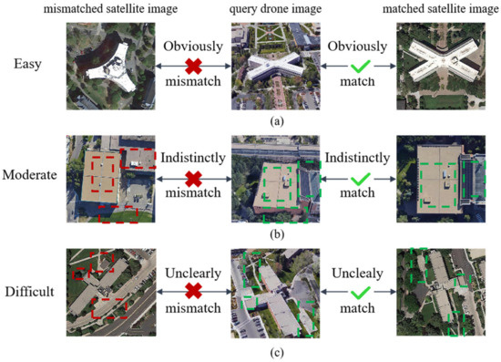
Figure 1.
The difficulty levels of matching different architectural scenes and the granularity of attention to specific regions during the matching process. (a) Easy judgment of whether there is a match. (b) Moderate judgment of whether there is a match. (c) Difficult judgment of whether there is a match.
Numerous deep learning methods aim to capture the overall semantic information of images. The latest research approach [4], leveraging the Vision Transformer [5], has improved the global correlation of local features, thereby enhancing image matching accuracy. However, existing methods predominantly focus on using single-scale features. Simultaneously, the use of a single-channel attention mechanism to correlate local features from different locations falls short in fully exploiting and utilizing multi-scale spatial structure information within the image, particularly in the extraction and utilization of locally valuable information. Based on previous research experience analysis, despite the multi-head self-attention module capturing global-range dependencies, making the receptive field of the Vision Transformer gradually more global midway through the network, the receptive field of the Vision Transformer also exhibits a strong dependence on the central patch. Therefore, as depicted in Figure 2, it can be observed that the regions emphasized by the pure Vision Transformer method [4] are more concentrated in the central part.
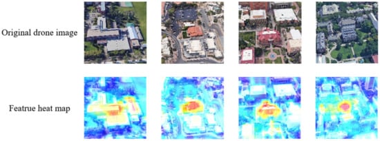
Figure 2.
The pure Vision Transformer method [4] extracts the heatmap of image features.
To address the shortcomings of existing methods, this paper proposes a novel framework called MIFT, which stands for Multi-scale Information Fusion based on Transformer. Specifically, MIFT achieves the fusion of multi-scale patch embeddings and multi-scale hierarchical features through the aggregation of convolutional features at different scales. This approach aims to extract detailed spatial structure and scene layout information at multiple scales. Additionally, MIFT utilizes self-attention mechanisms to capture global-to-local semantic information, enhancing image-level feature matching. The contributions of this paper can be summarized as follows:
- (1)
- We propose a Transformer-based cross-view geographic localization method, which integrates patch embeddings and hierarchical features separately to fully explore multi-scale contextual information.
- (2)
- A global–local range attention mechanism is designed to learn relationships among image feature nodes by employing different grouping strategies for patch embeddings, enabling the capture of overall semantic information in the image.
- (3)
- We substantiate the effectiveness of our approach on the University-1652 dataset and an independent self-made dataset. Our method demonstrates significantly superior localization accuracy compared to other state-of-the-art models. Code will be released at https://github.com/Gongnaiqun7/MIFT.
2. Related Works
- Cross-View Geolocalization
In recent years, cross-view geolocation has garnered increasing attention due to its vast potential applications. Before the advent of deep learning in the field of computer vision, some methods focused on utilizing manually designed features [6,7,8,9,10] to accomplish cross-view geolocation. Inspired by the tremendous success of Convolutional Neural Networks (CNNs) on ImageNet [11], researchers found that features extracted by deep neural networks could express higher-level semantic information compared to manually designed features. Current cross-view image geolocation mainly falls into two categories: matching ground images with satellite images and matching drone images with satellite images.
Early geolocation research primarily focused on ground images and satellite images. Workman [12] and others were the first to use two publicly available pretrained models to extract image features, demonstrating that deep features could differentiate images from different geographical locations. Lin [13] and others, inspired by face verification tasks, trained a Siamese AlexNet [14] network to map ground images and aerial images into a feature space, optimizing network parameters using contrastive loss functions [15,16]. Tian [17] employed Fast R-CNN to extract building features from images and designed a nearest neighbor matching algorithm for buildings. Hu [18] and others inserted NetVLAD [19] to extract discriminative features. Liu [20] and others found that azimuth information is crucial for spatial localization tasks. Zhai [21] and others utilized the semantic segmentation map to help semantic alignment. Shi [22] and others believed that existing methods overlooked the appearance and geometric differences between ground views and satellite views, approximating the alignment of satellite views with ground views using polar coordinate transformation. Regmi [23] and others applied Generative Adversarial Networks [24] (GANs) to cross-view geolocation, synthesizing satellite views from ground views using GANs for image matching. Zhu [25] and others obtained the rough geographic location through retrieval and refined the image’s geographic location by predicting offset through regression. The above research mainly focuses on the cross-view geolocation task between early ground-based and satellite images, primarily bridging the impact caused by spatial domain differences from the perspective transformation aspect.
Recent research results indicate that feature representation is crucial for model performance. Additionally, in recent years, studies on cross-view image geolocation suggest that increasing viewpoints can enhance geolocation accuracy. Therefore, researchers have introduced drone images and attempted to capture various robust features to address geolocation challenges. Zheng [26] and others constructed the University-1652 dataset, comprising satellite images, ground images, and drone images. They treated all view images from the same location as one category and employed a classification approach to accomplish geolocation tasks. They optimized the model using instance loss [27] and validation loss. Ding [28] achieved matching between drone images and satellite images through location classification, addressing the issue of imbalanced samples between satellite and drone images. Wang [29] proposed a ring partition strategy to segment feature images, making the network focus on the surroundings of target buildings, thereby obtaining more detailed information and achieving significant performance improvements on the University-1652 dataset. Tian [30] considered the spatial correspondence between drone-satellite views and surrounding contextual information, obtaining more context information. Zhuang [31] introduced a multi-scale attention structure to enhance salient features in different regions. Dai [4] achieved automatic region segmentation based on the heat distribution of Transformer feature maps, aligning specific regions in different views to improve the model’s accuracy and robustness to location variations. Zhuang [32] proposed a Transformer-based network to match drone images with satellite images. This network classifies each pixel in the image using pixel-wise attention, matching the same semantic parts in two images.
- B.
- Multi-scale Representation
Multi-scale representation refers to the sampling of signals at different granularities. Typically, different features can be extracted at different scales, allowing for the completion of various tasks. FPN [33] achieves the fusion of features at different scales by constructing a pyramid-shaped feature map. HRNet [34] employs parallel branches at multiple resolutions, coupled with continuous and bidirectional information exchange between branches, to simultaneously achieve semantic and precise positional information. PANet [35] introduces a path aggregation mechanism, which effectively captures the correlated information between multiscale features. Among them, FPN is the most popular one in practical use for its simplicity and universality; however, existing FPN directly collects multi-scale features from the original image, which has limitations. This study attempts feature-level optimization to enhance the capability of multi-scale feature representation.
- C.
- Attention Mechanism
The attention mechanism, as an effective means of feature selection and enhancement, has been widely applied across various domains of deep learning. Models structured around attention mechanisms not only capture positional relationships among information but also measure the importance of different features based on their respective weights. The Transformer [36] model achieves global sequence modeling through self-attention mechanisms. BERT [37], utilizing bidirectional Transformer encoders for pre-training, demonstrates remarkable performance across various natural language processing tasks. GPT [38] employs autoregressive Transformer decoders to excel in language generation tasks. Self-Attention [39] models introduce structured self-attention mechanisms, effectively capturing crucial information within input sequences. Recently proposed, the Swin Transformer [40] model achieves performance comparable to Transformer models in natural language processing, leveraging hierarchical attention mechanisms and shifted windows in the domain of image processing. Collectively, these contributions advance the development of attention mechanisms, endowing diverse tasks with robust modeling capabilities and yielding breakthroughs in fields such as natural language processing and computer vision.
3. Proposed Method
In this section, we introduce the details of our proposed method including the complete network structure, as shown in Figure 3. MIFT consists of three components. The first component, MEFF module, constructs multi-scale features. The second component, GLRA module, establishes feature correlations from a global to local scope. The third component, Segmentation Alignment Branch, accomplishes pixel-level feature matching.
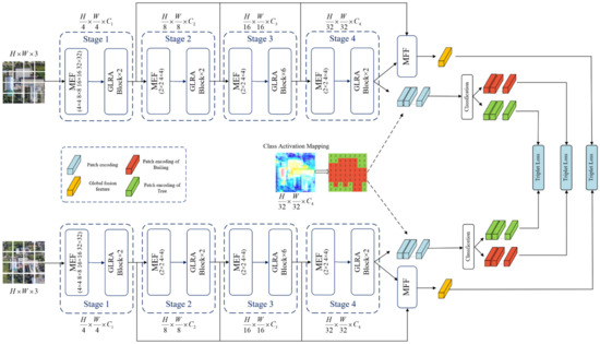
Figure 3.
The framework of the proposed method.
3.1. Network Architecture Overview
In this section, we introduce our proposed method, MIFT, and the complete network structure is illustrated in Figure 3. Firstly, the image is input into the multi-scale embedding fusion module (MEF), which generates multi-scale embeddings by taking the output of the previous stage (or input image) as input. Subsequently, several global–local range attention modules (GLRA) are added after MEF to explore the global structural information and local details of the image. Finally, the features extracted at different stages are input into the multi-scale feature fusion module (MFF). Additionally, a semantic segmentation branch is designed to achieve alignment of different semantic parts from two viewpoints. During the training process, metric learning is employed, and triplet loss is applied to each branch to minimize the distance between features with the same content. In the testing process, Euclidean distance is used to calculate the similarity between the query image and the database images. The retrieved images are then ranked based on their similarity.
3.2. Multi-Scale Embedding and Feature Fusion (MEFF)
In constructing multi-scale information, we perform fusion separately for patch embedding and hierarchical features. Regarding patch embedding, Figure 4a illustrates representations at different scales for two embeddings. It can be observed that solely considering the representation at a small scale makes it challenging to discern the relationship between the two embeddings, making it difficult to establish dependencies. Conversely, representation at a larger scale can provide rich semantic information to establish associations. Traditional Transformer variant networks such as Swin [40] and PVT [41] typically employ a single size of convolutional kernel for sampling at each stage of embedding construction. However, they may fail to establish strong dependencies between different embeddings. So, this paper constructs embeddings by considering multi-scale patches, achieved through multi-scale convolution followed by aggregation. For each central position, different-sized convolutional kernels are used to convolve with patches at different scales around this central position. The results are then concatenated, with the strides of different convolutions being the same. Taking the MEF in Stage 1 as an example, it takes the image as input and uses four convolutional kernels of different sizes for sampling. The strides and padding of these four kernels are controlled to generate the same number of embeddings. Different projection dimensions are set for each scale to control the overall budget of MEF, with the projection dimension inversely proportional to the kernel size. The specific numerical settings are provided in Figure 4b and its sub-table. Two different convolutional kernels (2 × 2 and 4 × 4) are used in other stages. Inspired by pyramid-structured models like Swin and PVT, the strides of MEF in other stages are set to 2 × 2 to reduce the number of embeddings to one-fourth.
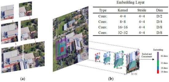
Figure 4.
(a) The representations of embeddings at different sizes. (b) Schematic diagram of the MEF module (using the first stage as an example). The input image is sampled by four different convolutional kernels (4 × 4, 8 × 8, 16 × 16, 32 × 32), all with the same stride (4 × 4). Consequently, each embedding is constructed by considering patches at four different scales.
For the feature fusion module, we employ deep features to weight shallow features within the module and then concatenate the deep features with the weighted shallow features. As illustrated in Figure 5, we follow common practices [42,43,44] by using four 1 × 1 convolutional layers to reduce the dimensionality of the output features from the four stages. The channel numbers are reduced from 768, 384, 192, and 96 to 512, 128, 64, and 64, respectively. Prior to weighting and fusion, shallow features undergo downsampling and convolution. We define a series of 3 × 3 convolutions with batch normalization [45] and ReLU [46] activation functions to process shallow features. The specific parameters for the convolutional layers (Convn) are detailed in Table 1.
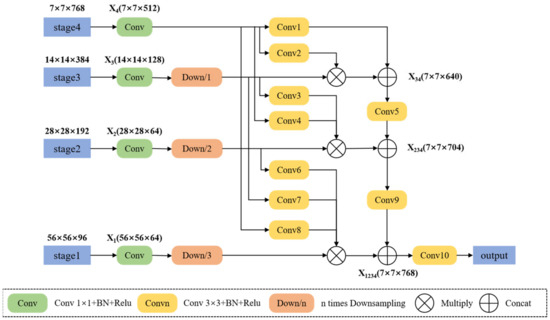
Figure 5.
Schematic diagram of the MFF module.

Table 1.
Convolutional Layer Parameters in the MFF Module.
3.3. Global–Local Range Attention (GLRA)
In order to address the Transformer’s tendency to capture more global dependencies and considering the challenge of increased computational complexity due to the large number of embeddings generated when using smaller convolutional kernels for multi-scale embedding, we devised a global–local range attention mechanism (GLRA). This mechanism aims to capture rich semantic information and fine-grained features in images. For local range attention, like Swin, our method also performs attention within a window range. We group adjacent t × t embeddings, resulting in multiple sets of local information. Taking Figure 6a as an example, by reshaping the original feature map of size 4 × 4 × C, we obtain four groups of 2 × 2 × C embeddings, which are then subjected to attention computation. We believe that performing attention within a moving window range in the Swin model could lead to increased computational complexity and a potential concentration of attention on a few positions within the input sequence, thereby neglecting information from other positions. Therefore, for global-range attention, we employ a fixed stride (e.g., 2 or 3) to sample rows and columns of the original feature map, producing multiple sets of global information. Illustrated in Figure 6b, for the original 4 × 4 × C feature map, using a 1 × 1 convolutional layer with a stride of 2, we similarly obtain four groups of 2 × 2 × C embeddings for attention processing. Since adjacent pixel positions in an image convey similar information, the GLRA provides a global receptive field, resulting in an almost global attention. Finally, the entire Transformer block is formed by stacking two self-attention blocks. Both self-attention blocks operate based on windows and employ the same attention computation as in Vision Transformer (ViT), with the constraint that self-attention computation is restricted to within each group. As shown in Figure 6c, the main distinction lies in the grouping strategy: one considers local information while the other considers global information. This structural design effectively leverages comprehensive global information to aid in matching images from the same geographical location.
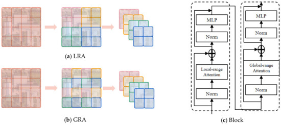
Figure 6.
(a) Local range attention. (b) Global range attention. (c) Transformer block.
3.4. Semantic Segmentation and Pixel Alignment
Although extracting robust global features at multiple scales is crucial, previous research has highlighted the importance of part-based methods for image retrieval [4,29,32]. Aligning specific semantic parts in images is a simple way to implement an end-to-end trained part-based approach. Without introducing additional supervisors, we perform pixel-level alignment between different semantic information in two-view images based on the heat map of the stage 4 feature map. Firstly, we calculate the heat value for each patch. The feature map of Stage 4 can be represented as , with a size of 1 × 49 × 768 (where 1 represents batch size, 49 represents the number of patches, and 768 represents the dimension, i.e., the length of the feature vector for each patch). By averaging the feature vectors of each patch, we obtain the heat value for each patch, which can be expressed as follows:
In the formula, represents the heat value of the j-th patch, and represents the i-th value of the feature vector corresponding to the j-th patch. After these operations, the size of is 1 × 49 × 1. The result is shown in Figure 7a.
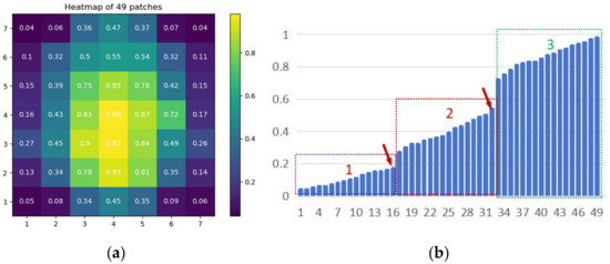
Figure 7.
(a) Heat values of each patch. (b) Region partition rules.
Subsequently, we sorted the heat values of in ascending order, as illustrated in Figure 7b. We calculated the gradient changes between adjacent patches, identified the n − 1 patches with the maximum gradient changes as breakpoints, and then divided all patches into different regions (n) based on the positions of these breakpoints. Each region was labeled as a distinct category. Taking , which divides all patches into three parts, as an example, through computation, we identified the two positions with significant gradient changes indicated by the red arrows in Figure 7b. Consequently, at these positions, we classified all patches into three categories: purple patches were labeled as trees, red patches as roads, and green patches as buildings. The entire process can be represented using the argmax function and first-order central differences:
After the aforementioned operations, we divided all patches into n regions based on the values of the heat map. As is well-known, directly using class labels may not be efficient for classification. Therefore, it is necessary to transform the data into feature vectors and input them into the classifier layer. Thus, we performed pooling operations on patches of different categories to obtain the feature vector . The expression for is as follows:
where n represents the number of different regions, is the feature vector of the j-th patch in the i-th region, and is the total number of patches in the i-th region. In short, is obtained by averaging pooling operations on all patches of each region. After these steps, we obtain feature vectors for the corresponding regions, and then classify each feature vector using the Classifier Layer. Thus, we obtain pixel-level local feature representations for different semantic parts in the image.
3.5. Loss Function and Learning Strategy
Cross-view image geolocalization can be fundamentally considered as an image retrieval task. Image retrieval is a feature matching problem, and instead of treating each target as a separate category, transforming the image retrieval problem into an image classification problem, metric learning aims to make the features of the same category more similar and those of different categories more distinct. This optimization approach is more direct. Therefore, this paper employs triplet loss to minimize the distance between feature vectors of the same category under different perspectives. Following previous studies [4,47], the traditional Euclidean distance is used and defined as follows:
In the equation, represents the 2-norm, is the feature vector of the query image ‘a’, is the feature vector of an image with the same category as ‘a’, and is the feature vector of an image with a different category to ‘a’. In our experiments, we computed the triplet loss with a threshold M = 0.3. To enable the model to establish more accurate matching relationships, we applied the triplet loss to all regions to reduce the distance between regions, as illustrated in Figure 3, where the triplet loss is applied to all positions. This includes both the multi-scale global features, serving as the image-level output, and the pixel-level output of various semantic local features.
It is worth noting that the task of cross-view image geolocation involves matching images from different perspectives rather than distinguishing images from the same perspective. Therefore, we only apply the triplet loss between different views. For instance, as illustrated in Figure 8, we extract an image from the light green set (drone or satellite view) and calculate triplet loss with all images from the light purple set (satellite or drone view).
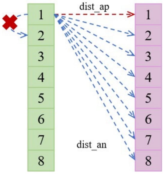
Figure 8.
Calculation of triplet loss. The numbers 1–8 represent the categories of images. The light green set represents 8 drone views or satellite views, and the light purple set represents 8 satellite views or drone views. dist_ap represents the distance between images of the same category; dist_an represents the distance between images of different categories. The red ‘×’ indicates that the distance between images from the same perspective is not calculated.
4. Experiment
In Section 4.1, we first introduce the public large-scale cross-view geolocalization datasets and evaluation protocols used in our experiments. Then, in Section 4.2, the implementation details are described. Next, the comparison with state-of-art methods is given in Section 4.3, followed by ablation studies in Section 4.4.
4.1. Datasets and Evaluation Metrics
4.1.1. University-1652 Dataset
In this work, we utilized the University-1652 dataset, as published by Zheng et al. [26]. Unlike constructing ground panoramic images to match satellite images in CVUSA [48] and CVACT, this dataset is unique in that it is the only benchmark dataset with both satellite and drone view images of buildings. The dataset comprises 1652 geographic targets from 72 universities worldwide. Each target includes three views: satellite view, drone view, and ground view. To mitigate the high cost of aerial control and drone flight, all drone and ground views were collected using a 3D engine named Google Earth, while satellite view images were obtained from Google Maps. The drone’s perspective in Google Earth is controlled through simulated camera angle adjustments, with the viewpoint height ranging from 256 m to 121.5 m. Each target consists of 1 satellite image, 54 drone images, and a small number of ground images.
The dataset is divided into a training set and a test set. The training set includes 701 buildings from 33 universities, while the test set includes 951 buildings from 39 universities. There is no overlap between the two sets. The original size of the captured images is 512 × 512 pixels. It is worth noting that, for testing in the drone-to-satellite view target localization task, the query image set consists of 37,855 drone view images and 701 true-matching satellite view images. The gallery contains 250 satellite view interference images, with only one true-matching satellite view image under this configuration. In the satellite-to-drone view navigation task, the gallery has 701 satellite view query images, 37,855 true-matching drone view images, and 13,500 drone view interference images. The specific distribution of each data group is shown in Table 2. Sample images from the dataset are illustrated in Figure 9.

Table 2.
Distribution of image data in University-1652.
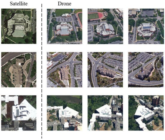
Figure 9.
Sample images from the University-1652 Dataset.
4.1.2. Self-Made Dataset
Due to the fact that all the drone images in the University 1652 dataset were extracted from 3D models, it may not be sufficient to prove its applicability in real drone scenarios. To further validate the model’s generalization ability in different scenarios, we captured aerial images of 42 buildings in the University Town of West Coast New Area, Qingdao, Shandong Province, China. Additionally, we obtained corresponding satellite images from Google Earth. Furthermore, we augmented the dataset with 30 additional drone and satellite images as distractor images for validation purposes. An example of the samples is depicted in Figure 10.
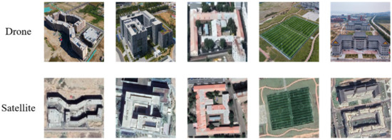
Figure 10.
Sample Images from the self-made Dataset.
4.1.3. Evaluation Protocols
In our experiments, Recall@K (R@K) and Average Precision (AP) are employed to evaluate the performance of the model. Higher values of R@K and AP indicate superior model performance. R@K is determined by calculating the proportion of truly matched images within the top K results in the ranking list. The computation formula is expressed as follows:
In this context, n represents the number of images in the query set. For a given query image with index i, the value of is 1 if the top K ranked results include the true matching images and 0 otherwise. Common choices for K include 1, 5, 10, and 1% of the total number of images in the reference image library. The accuracy is considered the most crucial metric in this evaluation.
AP (Average Precision) is a commonly used metric to measure the precision of retrieval systems. The calculation is expressed as follows:
In this context, n represents the number of images in the candidate image library. P(k) denotes the precision of the top k results in the retrieval ranking. If the kth image is a correct match for the query image, takes the value of 1; otherwise, it is 0. represents the total number of query images with true matches in the candidate image library.
4.2. Implementation Details
In data preprocessing, the training images are resized from 512 × 512 to 224 × 224, and random flips and random cropping augmentations are applied. Considering that each category has only one satellite image, we employ a multiple sampling strategy by expanding the satellite set through image augmentation to alleviate the imbalance of images from different domains, as detailed in Section 4.4.4. During training, we use stochastic gradient descent (SGD) as the optimizer with a momentum of 0.9 and weight decay of 0.0005 to optimize the model. For the initial learning rate, the backbone parameters are set to 0.003, and the rest of the learnable parameters are set to 0.01. After 100 and 120 iterations, the learning rate for all parameters is reduced to one-tenth of the original, and the model is trained for a total of 200 iterations. Regarding parameter initialization, we apply Kaiming initialization [49] to the classifier module. In testing, we utilize Euclidean distance to measure the similarity between the query image and candidate images in the image library. Our model is implemented using the PyTorch framework, and all experiments are conducted on an NVIDIA RTX A6000 GPU with 64 GB of memory (Nvidia Corporation, Santa Clara, CA, USA).
4.3. Comparison with Other Methods
4.3.1. Quantitative Statistics
On the University-1652 dataset, our proposed MIFT is compared with several existing competitive methods. As shown in Table 3, all our experiments utilize only drone views and satellite views from the dataset. In the Drone->Satellite task, R@1 is 87.84% and AP is 89.62%. In the Satellite->Drone task, R@1 is 92.30% and AP is 87.66%. Its performance surpasses advanced methods such as LPN [29], FSRA [4], SGM [32], and PAAN [50].

Table 3.
The comparison with other state-of-the-art results on the University-1652 dataset.
On the self-made dataset, the accuracy exhibits a trend similar to that on the University-1652 dataset: our method outperforms the aforementioned two methods. The results are shown in Table 4. In the Drone->Satellite task, R@1 is 77.44% and AP is 78.53%. In the Satellite->Drone task, R@1 is 75.08% and AP is 76.53%. We believe that the reason for the accuracy being lower than that on the University-1652 dataset is due to the resolution of satellite images. In comparison to the satellite images in the University-1652 dataset, the top information of buildings in the self-made dataset’s satellite images is somewhat blurry, which may affect the extraction of Fine-grained features and result in a decrease in retrieval accuracy.

Table 4.
The retrieval results on the self-made dataset.
4.3.2. Qualitative Analysis
As a qualitative assessment of the effectiveness of the multi-scale fusion method, we present the heatmaps of the final output feature maps from the network backbone MFF. Through these heatmaps, we observe a substantial difference in considering multi-scale features compared to other methods. As shown in Figure 11, Transformer-based methods with attention mechanisms allow the network to focus on global information, but more attention is concentrated on the central small area. This limitation results in the original ViT model struggling to segment the entire image effectively based on semantic information. In contrast, our approach pays more attention to the entire scene, showing a more significant segmentation effect for buildings, roads, and trees.
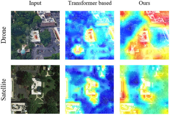
Figure 11.
On the left is the original image, in the middle is the heatmap from the last layer of ViT, and on the right is the heatmap from the last layer of multi-scale ViT.
In addition, we visualize the retrieval results for both the drone view target localization task and the drone navigation task, as shown in Figure 12. Each row represents the retrieval results for a target location. The first image is the query image, and the dashed line to the right shows the top five most closely matched images from the gallery set. The green box indicates correctly matched images, while the red box indicates incorrectly matched images. For the drone view target localization task, in Figure 12a, only one out of the top five matched images is a true satellite match. This demonstrates that our method can accurately retrieve matching images even in the presence of interference from similar images. For the drone navigation task, in Figure 12b, all top five matched images are correctly matched drone images, as each satellite image has 54 matching drone images associated with it. In addition, we visualize the retrieval results on the self-portrait dataset, as shown in Figure 12c,d. Unlike the retrieval results on the University-1652 dataset, where multiple aerial images were available for each building, the self-portrait dataset contains only one aerial image per building. Therefore, in both the drone localization and drone navigation tasks, only one true match image is present among the top five displayed matching results.
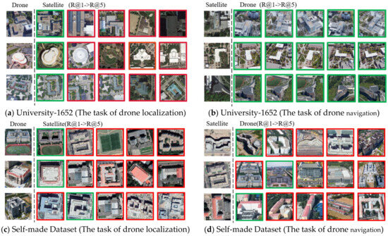
Figure 12.
Image retrieval results. (a) Top 5 retrieval results for drone target localization task on University-1652 dataset. (b) Top 5 retrieval results for drone navigation task on University-1652 dataset. (c) Top 5 retrieval results for drone target localization task on the self-made dataset. (d) Top 5 retrieval results for drone navigation task on the self-made dataset. Green boxes indicate correctly matched images, while red boxes indicate incorrectly matched images.
4.4. Ablation Studies
4.4.1. Effect of Different MEF’s Kernel Size
To validate the effectiveness of the multi-scale fusion embedding layer, we conducted experiments using a single-scale embedding layer. As shown in Table 5, when using a single-scale embedding layer (4 × 4 convolutional kernel), the model’s performance is enhanced with the multi-scale fusion embedding layer. Additionally, we experimented with various combinations of kernel sizes, which demonstrated similar performance. In conclusion, the multi-scale fusion embedding layer provides significant performance gains, and the model exhibits relative robustness to different kernel size choices.

Table 5.
Comparison between single-scale embedding layer and multi-scale fusion embedding layer, as well as the contrast between different kernel sizes.
4.4.2. Effect of Global–Local Range Attention
To validate the effectiveness of the global–local range attention, we compared our approach with two existing Transformer-based self-attention modules, namely, PVT and Swin. Specifically, PVT sacrifices small-scale features when computing self-attention, while Swin confines self-attention to a local range, foregoing the advantage of Transformer in extracting global features. As shown in Table 6, our designed GLRA outperforms self-attention mechanisms like PVT and Swin. The results indicate that employing global–local range self-attention is beneficial for enhancing the model’s performance.

Table 6.
Comparison of GLRA with other self-attention mechanisms.
4.4.3. Effect of the Number of Regions in Segmentation Branch
In our pixel-level matching branch, we partition the semantic categories of patches into n regions. When n = 2, the image is divided into two parts: buildings (foreground) and the environment (background). As illustrated in Figure 13, experimental results demonstrate that the model achieves optimal performance when n = 3, corresponding to the segmentation of the image into buildings, trees, and roads. It is noteworthy that when n = 1, the model solely relies on the multi-scale global features extracted by MIFT for cross-view image matching.
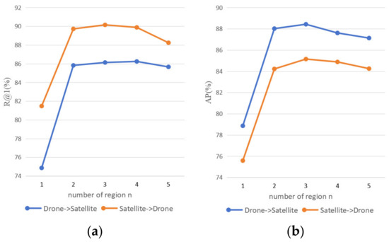
Figure 13.
The impact of different regions (n) on the task is depicted in the graphs: (a) represents the effect of n on R@1; (b) represents the impact on AP.
4.4.4. Effect of the Number of Sampling
In the University-1652 dataset, the correspondence ratio between one satellite view and 54 drone views is highly imbalanced. Inspired by methods such as LCM and FSRA, which use upsampling strategies for satellite image expansion, we introduced a hyperparameter k, representing the number of samples. Initially, we exported satellite views from the University-1652 dataset and augmented them to generate k enhanced satellite images. Augmentation techniques included random shifting, random cropping, and random flipping. Simultaneously, we randomly selected k images from other perspectives belonging to the same category as the corresponding satellite view. As shown in Table 7, the overall performance of the model is optimized when k is set to 3.

Table 7.
When the sampling count is k = 3, both R@1 and AP achieve the best performance in the two tasks.
4.4.5. Complexity Comparison of Different Models
Throughout the entire model, the attention mechanism is the most time-consuming module and also the most crucial part of the model. Therefore, we compare four types of attention mechanisms theoretically and empirically. Assuming the input size is s × s, the MHA complexity would be . Due to the fact that PVT reduces the length and width of key (K) and value (V) by a factor of 1/R, the complexity is decreased by times. As mentioned earlier, our method, like Swin, is also based on conducting attention within windows. Therefore, assuming the convolutional stride is t, with each window size being n × n (), with the global–local range attention mechanism, the complexity is reduced to . While the computational complexity of GLRA and Swin is in the same order of magnitude, Swin involves two additional shift operations and one mask operation. Additionally, we compared the computation time for inferring 10 images under each of the four types of attention mechanisms within the same network architecture and running environment (CPU RTX4060, CPUs AMD Ryzen-9-7945HX, Memory 16 G (AMD, Santa Clara, CA, USA)). The results are shown in Table 8. The run times of the four types of models follow well with the theoretical analysis.

Table 8.
The complexity comparison of the four attention mechanisms.
5. Conclusions
This paper proposes a Transformer-based cross-view geolocation method with multi-scale features. The method utilizes multi-scale patch embedding fusion, multi-scale hierarchical feature fusion modules, and a global–local range attention module to explore both overall semantic information and spatial geometric details of images. This allows the extraction of more robust multi-scale features for feature matching. Additionally, a semantic alignment branch based on weakly supervised segmentation is designed to perform pixel-level matching by aligning identical semantic information in different view images. Experimental results demonstrate the effectiveness of our method on the cross-view geolocation dataset University-1652, with significantly higher localization accuracy compared to other state-of-the-art models.
In future research, we plan to consider the continuity and complexity of images in real-world scenarios, further investigating cross-view geolocation methods adapted to complex scenes and exploring ways to enhance accuracy in cross-view image geolocation.
Author Contributions
Conceptualization, N.G. and J.S.; methodology, N.G. and L.L.; validation, Q.H.; formal analysis, N.G.; resources, J.S.; writing—original draft preparation, N.G. and L.L.; writing—review and editing, N.G. and J.S.; visualization, Q.H.; supervision, X.S.; project administration, L.L. and J.S.; funding acquisition, L.L. and J.S. All authors have read and agreed to the published version of the manuscript.
Funding
This research was funded by the National Natural Science Foundation of China (grant number 41971327) and Aerospace Innovation and Development Fund Project (grant ZY0110020009).
Data Availability Statement
Data are contained within the article.
Conflicts of Interest
The authors declare no conflicts of interest.
References
- Shetty, A.; Gao, G.X. UAV Pose Estimation Using Cross-View Geolocalization with Satellite Imagery. In Proceedings of the 2019 International Conference on Robotics and Automation (ICRA), Montreal, QC, Canada, 20–24 May 2019; pp. 1827–1833. [Google Scholar]
- Long, Y.; Gong, Y.; Xiao, Z.; Liu, Q. Accurate Object Localization in Remote Sensing Images Based on Convolutional Neural Networks. IEEE Trans. Geosci. Remote Sens. 2017, 55, 2486–2498. [Google Scholar] [CrossRef]
- Kim, D.-K.; Walter, M.R. Satellite Image-Based Localization via Learned Embeddings. In Proceedings of the 2017 IEEE International Conference on Robotics and Automation (ICRA), Singapore, 29 May–3 June 2017; pp. 2073–2080. [Google Scholar]
- Dai, M.; Hu, J.; Zhuang, J.; Zheng, E. A Transformer-Based Feature Segmentation and Region Alignment Method for UAV-View Geo-Localization. IEEE Trans. Circuits Syst. Video Technol. 2022, 32, 4376–4389. [Google Scholar] [CrossRef]
- Dosovitskiy, A.; Beyer, L.; Kolesnikov, A.; Weissenborn, D.; Zhai, X.; Unterthiner, T.; Dehghani, M.; Minderer, M.; Heigold, G.; Gelly, S.; et al. An Image IS Worth 16 × 16 Words: Transformers for Image Recognition at Scale. arXiv 2021, arXiv:2010.11929v2. [Google Scholar]
- Castaldo, F.; Zamir, A.; Angst, R.; Palmieri, F.; Savarese, S. Semantic Cross-View Matching. In Proceedings of the 2015 IEEE International Conference on Computer Vision Workshop (ICCVW), Santiago, Chile, 7–13 December 2015. [Google Scholar]
- Lin, T.-Y.; Belongie, S.; Hays, J. Cross-View Image Geolocalization. In Proceedings of the 2013 IEEE Conference on Computer Vision and Pattern Recognition, Portland, OR, USA, 23–28 June 2013; pp. 891–898. [Google Scholar]
- Senlet, T.; Elgammal, A. A Framework for Global Vehicle Localization Using Stereo Images and Satellite and Road Maps. In Proceedings of the 2011 IEEE International Conference on Computer Vision Workshops (ICCV Workshops), Barcelona, Spain, 6–13 November 2011; pp. 2034–2041. [Google Scholar]
- Bansal, M.; Sawhney, H.S.; Cheng, H.; Daniilidis, K. Geo-Localization of Street Views with Aerial Image Databases. In Proceedings of the 19th ACM International Conference on Multimedia, Scottsdale, AZ, USA, 28 November 2011; ACM: New York, NY, USA, 2011; pp. 1125–1128. [Google Scholar]
- Yu, J.; Rui, Y.; Tao, D. Click Prediction for Web Image Reranking Using Multimodal Sparse Coding. IEEE Trans. Image Process. 2014, 23, 2019–2032. [Google Scholar] [CrossRef] [PubMed]
- Deng, J.; Dong, W.; Socher, R.; Li, L.-J.; Li, K.; Li, F.-F. ImageNet: A Large-Scale Hierarchical Image Database. In Proceedings of the 2009 IEEE Conference on Computer Vision and Pattern Recognition, Miami, FL, USA, 20–25 June 2009; pp. 248–255. [Google Scholar]
- Workman, S.; Jacobs, N. On the Location Dependence of Convolutional Neural Network Features. In Proceedings of the 2015 IEEE Conference on Computer Vision and Pattern Recognition Workshops (CVPRW), Boston, MA, USA, 7–12 June 2015; pp. 70–78. [Google Scholar]
- Lin, T.-Y.; Cui, Y.; Belongie, S.; Hays, J. Learning Deep Representations for Ground-to-Aerial Geolocalization. In Proceedings of the 2015 IEEE Conference on Computer Vision and Pattern Recognition (CVPR), Boston, MA, USA, 7–12 June 2015; pp. 5007–5015. [Google Scholar]
- Chopra, S.; Hadsell, R.; LeCun, Y. Learning a Similarity Metric Discriminatively, with Application to Face Verification. In Proceedings of the 2005 IEEE Computer Society Conference on Computer Vision and Pattern Recognition (CVPR’05), San Diego, CA, USA, 20–25 June 2005; Volume 1, pp. 539–546. [Google Scholar]
- Hadsell, R.; Chopra, S.; LeCun, Y. Dimensionality Reduction by Learning an Invariant Mapping. In Proceedings of the 2006 IEEE Computer Society Conference on Computer Vision and Pattern Recognition—Volume 2 (CVPR’06), New York, NY, USA, 17–22 June 2006; Volume 2, pp. 1735–1742. [Google Scholar]
- Deng, W.; Zheng, L.; Ye, Q.; Kang, G.; Yang, Y.; Jiao, J. Image-Image Domain Adaptation with Preserved Self-Similarity and Domain-Dissimilarity for Person Re-Identification. In Proceedings of the 2018 IEEE/CVF Conference on Computer Vision and Pattern Recognition, Salt Lake City, UT, USA, 18–22 June 2018; pp. 994–1003. [Google Scholar]
- Tian, Y.; Chen, C.; Shah, M. Cross-View Image Matching for Geo-Localization in Urban Environments. In Proceedings of the 2017 IEEE Conference on Computer Vision and Pattern Recognition (CVPR), Honolulu, HI, USA, 21–26 July 2017; pp. 1998–2006. [Google Scholar]
- Hu, S.; Feng, M.; Nguyen, R.M.H.; Lee, G.H. CVM-Net: Cross-View Matching Network for Image-Based Ground-to-Aerial Geo-Localization. In Proceedings of the 2018 IEEE/CVF Conference on Computer Vision and Pattern Recognition, Salt Lake City, UT, USA, 18–23 June 2018; pp. 7258–7267. [Google Scholar]
- Arandjelovic, R.; Gronat, P.; Torii, A.; Pajdla, T.; Sivic, J. NetVLAD: CNN Architecture for Weakly Supervised Place Recognition. IEEE Trans. Pattern Anal. Mach. Intell. 2018, 40, 1437–1451. [Google Scholar] [CrossRef] [PubMed]
- Liu, L.; Li, H. Lending Orientation to Neural Networks for Cross-View Geo-Localization. In Proceedings of the 2019 IEEE/CVF Conference on Computer Vision and Pattern Recognition (CVPR), Long Beach, CA, USA, 15–20 June 2019; pp. 5617–5626. [Google Scholar]
- Zhai, M.; Bessinger, Z.; Workman, S.; Jacobs, N. Predicting Ground-Level Scene Layout from Aerial Imagery. In Proceedings of the 2017 IEEE Conference on Computer Vision and Pattern Recognition (CVPR), Honolulu, HI, USA, 21–26 July 2017; pp. 4132–4140. [Google Scholar]
- Shi, Y.; Liu, L.; Yu, X.; Li, H. Spatial-Aware Feature Aggregation for Cross-View Image Based Geo-Localization. In Proceedings of the 33rd International Conference on Neural Information Processing Systems, Vancouver, BC, Canada, 8–14 December 2019. [Google Scholar]
- Regmi, K.; Borji, A. Cross-View Image Synthesis Using Conditional GANs. In Proceedings of the 2018 IEEE/CVF Conference on Computer Vision and Pattern Recognition, Salt Lake City, UT, USA, 18–23 June 2018; pp. 3501–3510. [Google Scholar]
- Goodfellow, I.J.; Pouget-Abadie, J.; Mirza, M.; Xu, B.; Warde-Farley, D.; Ozair, S.; Courville, A.; Bengio, Y. Generative Adversarial Networks. Commun. ACM 2020, 63, 139–144. [Google Scholar] [CrossRef]
- Zhu, S.; Yang, T.; Chen, C. VIGOR: Cross-View Image Geo-Localization beyond One-to-One Retrieval. In Proceedings of the 2021 IEEE/CVF Conference on Computer Vision and Pattern Recognition (CVPR), Nashville, TN, USA, 20–25 June 2021; pp. 5316–5325. [Google Scholar]
- Zheng, Z.; Wei, Y.; Yang, Y. University-1652: A Multi-View Multi-Source Benchmark for Drone-Based Geo-Localization. In Proceedings of the 28th ACM International Conference on Multimedia, Seattle, WA, USA, 12–16 October 2020. [Google Scholar]
- Zheng, Z.; Zheng, L.; Garrett, M.; Yang, Y.; Xu, M.; Shen, Y.-D. Dual-Path Convolutional Image-Text Embeddings with Instance Loss. ACM Trans. Multimed. Comput. Commun. Appl. 2020, 16, 1–23. [Google Scholar] [CrossRef]
- Ding, L.; Zhou, J.; Meng, L.; Long, Z. A Practical Cross-View Image Matching Method between UAV and Satellite for UAV-Based Geo-Localization. Remote Sens. 2020, 13, 47. [Google Scholar] [CrossRef]
- Wang, T.; Zheng, Z.; Yan, C.; Zhang, J.; Sun, Y.; Zheng, B.; Yang, Y. Each Part Matters: Local Patterns Facilitate Cross-View Geo-Localization. IEEE Trans. Circuits Syst. Video Technol. 2022, 32, 867–879. [Google Scholar] [CrossRef]
- Tian, X.; Shao, J.; Ouyang, D.; Shen, H.T. UAV-Satellite View Synthesis for Cross-View Geo-Localization. IEEE Trans. Circuits Syst. Video Technol. 2022, 32, 4804–4815. [Google Scholar] [CrossRef]
- Zhuang, J.; Dai, M.; Chen, X.; Zheng, E. A Faster and More Effective Cross-View Matching Method of UAV and Satellite Images for UAV Geolocalization. Remote Sens. 2021, 13, 3979. [Google Scholar] [CrossRef]
- Zhuang, J.; Chen, X.; Dai, M.; Lan, W.; Cai, Y.; Zheng, E. A Semantic Guidance and Transformer-Based Matching Method for UAVs and Satellite Images for UAV Geo-Localization. IEEE Access 2022, 10, 34277–34287. [Google Scholar] [CrossRef]
- Lin, T.-Y.; Dollar, P.; Girshick, R.; He, K.; Hariharan, B.; Belongie, S. Feature Pyramid Networks for Object Detection. In Proceedings of the 2017 IEEE Conference on Computer Vision and Pattern Recognition (CVPR), Honolulu, HI, USA, 21–26 July 2017; pp. 936–944. [Google Scholar]
- Sun, K.; Xiao, B.; Liu, D.; Wang, J. Deep High-Resolution Representation Learning for Human Pose Estimation. In Proceedings of the 2019 IEEE/CVF Conference on Computer Vision and Pattern Recognition (CVPR), Long Beach, CA, USA, 15–20 June 2019. [Google Scholar]
- Liu, S.; Qi, L.; Qin, H.; Shi, J.; Jia, J. Path Aggregation Network for Instance Segmentation. In Proceedings of the 2018 IEEE/CVF Conference on Computer Vision and Pattern Recognition, Salt Lake City, UT, USA, 18–23 June 2018. [Google Scholar]
- Vaswani, A.; Shazeer, N.; Parmar, N.; Uszkoreit, J.; Jones, L.; Gomez, A.N.; Kaiser, Ł.; Polosukhin, I. Attention is all you need. Adv. Neural Inf. Process. Syst. 2017, 30. Available online: https://papers.nips.cc/paper_files/paper/2017/hash/3f5ee243547dee91fbd053c1c4a845aa-Abstract.html (accessed on 12 June 2017).
- Devlin, J.; Chang, M.-W.; Lee, K.; Toutanova, K. BERT: Pre-Training of Deep Bidirectional Transformers for Language Understanding. arXiv 2019, arXiv:1810.04805v2. [Google Scholar]
- Radford, A.; Narasimhan, K.; Salimans, T.; Sutskever, I. Improving Language Understanding by Generative Pre-Training. Available online: https://www.mikecaptain.com/resources/pdf/GPT-1.pdf (accessed on 11 June 2018).
- Lin, Z.; Feng, M.; dos Santos, C.N.; Yu, M.; Xiang, B.; Zhou, B.; Bengio, Y. A Structured Self-Attentive Sentence Embedding. arXiv 2017, arXiv:1703.03130. [Google Scholar] [CrossRef]
- Liu, Z.; Lin, Y.; Cao, Y.; Hu, H.; Wei, Y.; Zhang, Z.; Lin, S.; Guo, B. Swin Transformer: Hierarchical Vision Transformer Using Shifted Windows. In Proceedings of the 2021 IEEE/CVF International Conference on Computer Vision (ICCV), Montreal, QC, Canada, 10–17 October 2021. [Google Scholar]
- Wang, W.; Xie, E.; Li, X.; Fan, D.-P.; Song, K.; Liang, D.; Lu, T.; Luo, P.; Shao, L. Pyramid Vision Transformer: A Versatile Backbone for Dense Prediction without Convolutions. In Proceedings of the 2021 IEEE/CVF International Conference on Computer Vision (ICCV), Montreal, QC, Canada, 10–17 October 2021; pp. 548–558. [Google Scholar]
- Fan, D.-P.; Ji, G.-P.; Zhou, T.; Chen, G.; Fu, H.; Shen, J.; Shao, L. PraNet: Parallel Reverse Attention Network for Polyp Segmentation. In Proceedings of the Medical Image Computing and Computer Assisted Intervention—MICCAI 2020, Lima, Peru, 4–8 October 2020. [Google Scholar]
- Wu, Z.; Su, L.; Huang, Q. Cascaded Partial Decoder for Fast and Accurate Salient Object Detection. In Proceedings of the 2019 IEEE/CVF Conference on Computer Vision and Pattern Recognition (CVPR), Long Beach, CA, USA, 15–20 June 2019; pp. 3902–3911. [Google Scholar]
- Dong, B.; Wang, W.; Fan, D.-P.; Li, J.; Fu, H.; Shao, L. Polyp-PVT: Polyp Segmentation with Pyramid Vision Transformers. CAAI Artif. Intell. Res. 2023, 2, 9150015. [Google Scholar] [CrossRef]
- Ioffe, S.; Szegedy, C. Batch Normalization: Accelerating Deep Network Training by Reducing Internal Covariate Shift. In Proceedings of the 32nd International Conference on Machine Learning, ICML 2015, Lille, France, 6–11 July 2015. [Google Scholar]
- Glorot, X.; Bordes, A.; Bengio, Y. Deep Sparse Rectifier Neural Networks. In Proceedings of the 14th International Conference on Artificial Intelligence and Statistics, Fort Lauderdale, FL, USA, 11–13 April 2011. [Google Scholar]
- Chen, K.; Lei, W.; Zhao, S.; Zheng, W.-S.; Wang, R. PCCT: Progressive Class-Center Triplet Loss for Imbalanced Medical Image Classification. IEEE J. Biomed. Health Inform. 2023, 27, 2026–2036. [Google Scholar] [CrossRef] [PubMed]
- Workman, S.; Souvenir, R.; Jacobs, N. Wide-Area Image Geolocalization with Aerial Reference Imagery. In Proceedings of the 2015 IEEE International Conference on Computer Vision (ICCV), Santiago, Chile, 7–13 December 2015; pp. 3961–3969. [Google Scholar]
- He, K.; Zhang, X.; Ren, S.; Sun, J. Delving Deep into Rectifiers: Surpassing Human-Level Performance on ImageNet Classification. In Proceedings of the 2015 IEEE International Conference on Computer Vision (ICCV), Santiago, Chile, 7–13 December 2015. [Google Scholar]
- Bui, D.V.; Kubo, M.; Sato, H. A Part-Aware Attention Neural Network for Cross-View Geo-Localization between UAV and Satellite. J. Robot. Netw. Artif. Life 2022, 9, 275–284. [Google Scholar]
- Radenović, F.; Tolias, G.; Chum, O. Fine-Tuning CNN Image Retrieval with No Human Annotation. IEEE Trans. Pattern Anal. Mach. Intell. 2018, 41, 1655–1668. [Google Scholar] [CrossRef]
Disclaimer/Publisher’s Note: The statements, opinions and data contained in all publications are solely those of the individual author(s) and contributor(s) and not of MDPI and/or the editor(s). MDPI and/or the editor(s) disclaim responsibility for any injury to people or property resulting from any ideas, methods, instructions or products referred to in the content. |
© 2024 by the authors. Licensee MDPI, Basel, Switzerland. This article is an open access article distributed under the terms and conditions of the Creative Commons Attribution (CC BY) license (https://creativecommons.org/licenses/by/4.0/).