Abstract
In recent years, graph convolutional networks (GCNs) have attracted increasing attention in hyperspectral image (HSI) classification owing to their exceptional representation capabilities. However, the high computational requirements of GCNs have led most existing GCN-based HSI classification methods to utilize superpixels as graph nodes, thereby limiting the spatial topology scale and neglecting pixel-level spectral–spatial features. To address these limitations, we propose a novel HSI classification network based on graph convolution called the spatial-pooling-based graph attention U-net (SPGAU). Specifically, unlike existing GCN models that rely on fixed graphs, our model involves a spatial pooling method that emulates the region-growing process of superpixels and constructs multi-level graphs by progressively merging adjacent graph nodes. Inspired by the CNN classification framework U-net, SPGAU’s model has a U-shaped structure, realizing multi-scale feature extraction from coarse to fine and gradually fusing features from different graph levels. Additionally, the proposed graph attention convolution method adaptively aggregates adjacency information, thereby further enhancing feature extraction efficiency. Moreover, a 1D-CNN is established to extract pixel-level features, striking an optimal balance between enhancing the feature quality and reducing the computational burden. Experimental results on three representative benchmark datasets demonstrate that the proposed SPGAU outperforms other mainstream models both qualitatively and quantitatively.
1. Introduction
The rapid advancement in aerospace vehicle and optics technology has substantially improved hyperspectral imaging techniques [1], resulting in higher-quality and more cost-effective acquisition of hyperspectral images (HSIs) [2]. Each pixel within these images contains an abundance of spectral information, encompassing hundreds of distinct bands [3]. This extensive spectral information renders HSIs suitable for numerous practical applications, including environmental inspection [4], agricultural assessment [5], and military investigations [6]. The advantages of HSI extend to the capability of assigning specific land-cover labels to each hyperspectral pixel, hence promoting interest in HSI classification.
To address the challenge of HSI classification, various methods have been introduced [7]. In essence, HSI classification categorizes pixels by extracting image features, thereby emphasizing the need for discriminative feature extraction [8]. In the early stages, feature extraction methods were often manually designed using machine learning techniques, primarily based on spectral and spatial information found in spectral images. For example, methods like support vector machine (SVM) [9], logistic regression [10], linear discriminant analysis (LDA) [11], and principal component analysis (PCA) [12], which rely on spectral information, were proposed. However, these methods typically focus on HSI features while disregarding spatial information, resulting in less-than-ideal classification performance [13]. To enrich the feature space, it is imperative to harness spatial information in conjunction with spectral data in HSIs [14]. As a result, several spatial–spectral-based techniques, which consider both spatial and spectral information, have been developed. Among these, specific joint spatial–spectral classifiers leverage the characteristics of HSI data cubes. For instance, the utilization of 3-D wavelet analysis (WT) [15,16] and morphological information methods [17,18] is noteworthy. Furthermore, other methods place a higher emphasis on the spatial relationship between pixels, utilizing concepts like manifold learning [19], superpixel learning [20], and graph representation learning [21]. These techniques enable the construction of structural information within HSI data. While these methods have achieved considerable success in HSI classification, traditional machine learning classification methods are constrained by their reliance on human-crafted features and empirical parameters, which hinders in-depth feature extraction [22].
In comparison, deep learning (DL) can autonomously extract depth features through multi-layer neural networks [23,24]. Following their achievements in the realm of RGB images, DL models have been widely adopted in HSI classification due to their strong feature representation capabilities [25,26]. In their nascent stages, Chen et al. spearheaded the use of DL models for HSI classification by devising a stacked autoencoder for high-level feature extraction [27]. Subsequently, a plethora of DL classifiers for HSI classification have surfaced, achieving exceptional results. Notable examples include convolutional neural networks (CNNs) [28], recurrent neural networks (RNNs) [29], deep belief networks (DBNs) [30], and various other models. Among these deep learning approaches, CNNs have emerged as the most widely employed framework for HSI classification. The learning paradigms of CNN-based methods cover a variety of models, including transfer learning [31], meta-learning [32], active learning [33], and so on. Several CNN models with distinct architectures have been introduced to maximize the utilization of spectral and spatial data in HSIs, enhancing the network’s expressiveness by focusing on dimensions, network depth, and complexity. For example, Hu et al. pioneered the incorporation of the CNN model into HSI classification, developing a 1-D CNN classifier for spectral information extraction [34]. To leverage the spatial information in HSIs, Li et al. elevated the dimensionality of CNN, presenting a 3D-CNN model for extracting spectral–spatial features [35]. Additionally, the extraction of spectral–spatial features can be realized through multi-channel fusion, as exemplified by two-channel CNN (TCCNN) [36] and multi-channel CNN (MCCNN) [37]. Furthermore, inspired by the visual attention mechanism, attention techniques have been integrated into CNNs in various recent methods [38,39]. While existing CNN-based methods have made significant performance strides, the convolution operations in CNN models operate on regular square regions, neglecting pixel-to-pixel relationships. Although attention-based CNNs can assign different weights to distinct feature dimensions, they cannot directly evaluate pixel correlations due to CNN models’ inability to handle non-Euclidean data, such as the adjacency relationships between pixels.
Non-Euclidean spatial data pervade the real world. Graphs which connect vertices and edges offer a means to represent non-Euclidean data, with graph neural networks (GNNs) capable of directly extracting information from these graph structures [40]. Consequently, GNNs enable comprehensive extraction of spectral–spatial features in hyperspectral imaging (HSI) and yield impressive classification results. Presently, GNN approaches for HSI classification encompass three main methods of constructing graphs: pixel-based [41], selection region-based [42], and superpixel-based [43]. Among these, the pixel-based approach designates each pixel as a vertex, generating the graph structure based on all HSI pixels. Given the typically high resolution of HSIs, this method entails significant computational demands [41]. In contrast, the selection region-based approach constructs the graph using randomly chosen pixel patches from any HSI region rather than the entire HSI dataset. Hong et al. [42] effectively harnessed constructive relations and image features through a dual-channel mode employing GCNs and CNNs. On the other hand, superpixels contain adjacent pixels with similar features, making them a useful preprocessing tool for HSIs. They mitigate memory consumption and maintain the edge information of ground objects. Ren et al. devised superpixel adjacency graph structures at various scales and adapted these structures at each scale using feature similarity and nuclear diffusion. This approach facilitates high-level feature extraction while conserving computational resources [43]. While the former extracts multi-scale features by simultaneously constructing graph structures of different scales, our method evolves into multi-scale graph structures using the spatial pooling module, subsequently fusing features of varying scales throughout the U-shaped structure.
However, as discussed in [44], pixel-level graph nodes result in substantial computation. In response, a spatial-pooling-based graph attention neural network (SPGAU) is proposed for HSI classification. In this network, we use a superpixel-based method to preprocess the original HSI and greatly reduce the number of graph nodes. Moreover, to extract multi-scale spatial features from HSI, we design a spatial pooling module to obtain multi-scale maps. As the number of graph nodes decreases layer-by-layer, the computational burden gradually lightens. The primary contributions of this article are as follows:
- 1.
- We propose a novel spatial pooling module that emulates the process of superpixel merging and conducts random merging operations on neighboring nodes exhibiting high similarity in the graph. This operation not only reduces computational costs but also abstracts the multi-scale graph structure.
- 2.
- We incorporate an attention mechanism into the graph convolution network to enhance the efficacy of feature extraction.
- 3.
- We employ 1-D CNN to extract per-pixel image features, thus mitigating the potential loss of pixel-level information resulting from superpixel segmentation.
The remainder of the paper is structured as follows: In Section 2, we introduce the proposed SPGAU model. Section 3 describes three HSI classification datasets and experimental settings. In Section 4, we present a systematic discussion of the experimental results. Finally, Section 5 presents the conclusions and provides insight into future research directions.
2. Related Work
2.1. Graph Convolution
In recent years, graph neural networks (GNNs) have achieved state-of-the-art performance in various graph-related tasks by successfully extending convolution operators to graph-structured data. Existing GCN algorithms can be broadly categorized into two groups: spectral-based and spatial-based approaches. Spectral-based methods predominantly employ Fourier transforms and the graph Laplacian operator to define the convolution operation as a filter, with the goal of noise reduction in the graph signal. The ChebNet [45] algorithm, for instance, utilizes Chebyshev expansion for approximating k-polynomial filters, enhancing computational efficiency. GCN [46] simplifies the Chebyshev polynomial into a local spectrum filter, resulting in a first-order approximation of ChebNet. This approach enables weight and parameter sharing, significantly reducing complexity. To address the computational load associated with Laplacian matrix feature decomposition, the graph wavelet neural network (GWNN) [47] employs local wavelet transforms instead of global Fourier transforms for convolution operations. This strategy leverages the inherent sparsity in wavelet transforms, reducing network complexity. However, these models have limitations, such as their inability to handle directed graphs and their confinement to shallow networks.
In contrast to spectral-based methods, spatial-based methods do not rely on graph theory and directly aggregate neighborhood information for convolution operations. Given the inherent disarray in graph structures, GNN [48] utilizes a random walk method to determine node neighborhoods. However, when dealing with numerous neighboring nodes, using all neighbors for aggregation becomes inefficient. To tackle this challenge, GraphSAGE [49] samples a fixed number of neighbors for each node, significantly reducing computational costs. Additionally, the graph attention network (GAT) [50] introduces an attention mechanism to learn the weights between nodes, differentiating aggregation based on the importance of adjacent nodes. Nevertheless, these two branches of GCN mainly focus on learning node representations, making them incapable of generating more abstract graph representations due to the lack of subsampling operations.
2.2. Graph Pooling
Pooling operations in convolutional neural networks (CNNs) effectively reduce the size of input feature graphs and the number of training parameters, thereby enhancing model performance. Similarly, graph pooling techniques can also enhance model performance by suitably compressing nodes within a graph. Existing graph pooling methods can be categorized into global pooling and hierarchical pooling based on their roles in GNNs [51]. Global graph pooling captures node information representing the entire graph’s characteristics, often employed to link GNN layers with classifiers for more discriminative feature information in classification tasks. Common global graph pooling approaches include averaging and summing [45], attention mechanisms [52], feature sorting, and splicing [53]. Hierarchical graph pooling mirrors traditional CNN-based pooling, focusing on capturing the topological structure of a given graph while learning multi-scale information through structural modifications. Hierarchical graph pooling is analogous to traditional convolutional neural network pooling, with a primary focus on capturing the topological structure of the graph and learning multi-scale information by modifying the graph’s structure. Hierarchical pooling can be broadly classified into two approaches: graph coarsening [54] and node selection [55]. Graph coarsening methods aim to map nodes to distinct clusters and condense the graph into a higher-level substructure. On the other hand, node selection methods involve evaluating individual nodes or edges between nodes to determine which should be merged or eliminated.
3. Methodology
In this section, we initially outline the overall framework of SPGAU. Subsequently, we elucidate the method for constructing superpixel graphs. Moreover, we provide a concise introduction to the attention-based graph convolution module employed in our approach. Finally, we present the spatial pooling module, which interconnects the graph convolutional modules to evolve the graph structure.
3.1. Overview of the SPGAU
We propose a spatial-pooling-based graph attention neural network (SPGAU), as illustrated in Figure 1. Initially, the original HSI is divided into local patches (superpixels). Simultaneously, to enhance the learning capacity for pixel-level subtle features, a 1D-CNN is introduced for the efficient extraction of superpixel spectral features. Furthermore, an attention mechanism is integrated into the graph convolution process to adaptively aggregate feature efficiency. The similarity between nodes provides a similarity measure for the node merging in the spatial pooling module. Through the superpixel merging process, spatial pooling generates a more abstract graph structure by merging nodes with high similarity. In contrast to fusing features of different scales concurrently, the feature fusion of our spatial-pooling-based graph attention U-Net (SPGAU) unfolds gradually from shallow to deep layers, optimally using the U-Net structure to fuse information across various scales, naturally aligning with the pixel-level classification task in HSI.
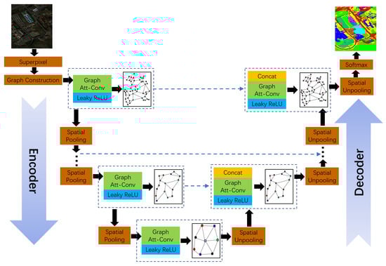
Figure 1.
The conceptual architecture of SPGAU. Firstly, the superpixels obtained by hyperspectral image segmentation (SLIC) are used as graph nodes, the hidden states of the nodes are the feature vectors extracted by the convolutional neural network, and the graph is constructed according to the spatial relationship between the superpixels. Then, multi-scale feature information is extracted by graph evolution through a set of stacked graph attention convolution and spatial pooling modules. Finally, the segmentation result of HSI is obtained by the softmax function. The blue dashed line indicates the skip connection, and the black arrow is the direction of the information flow.
3.2. Graph Construction
Hyperspectral images typically encompass hundreds of thousands of pixels, with each pixel containing hundreds of spectral channels. The vast amount of image data exerts significant computational demands on HSI classifiers. To mitigate this computational complexity while retaining the local structure and feature information in the image, we apply the simple linear iterative clustering (SLIC) [56] technique for segmenting HSI into spatially connected superpixels. Each superpixel is considered a node; then, an undirected graph is constructed depending on the adjacency relationships between superpixels in the HSI. Here, denotes the nodes, and represents the edges. Typically, these are portrayed using the superpixel adjacency matrix A and node feature matrix H , where F represents the number of superpixels, and D is the feature dimension. According to the position relationship of the superpixels in graph , the superpixel adjacency matrix A can be defined as
where represents the ith superpixel, consisting of several HSI pixels , and signifies the number of pixels in .
In practice, the noise of the hyperspectral images interferes with the reliability of the features of the superpixels. To suppress the noise, we use 1D-CNN to perform convolution operations on the spectral channel of HSI, and the feature of the bth spectral channel of the pixel is denoted as
where is the original spectral value of the bth channel at pixel , and are the learnable weights and bias. Then, the spectral feature vector can be written as
where B is the number of spectral channels. Finally, we compute the average features of a superpixel as a node vector, and the graph node feature matrix H can be mathematically calculated as
3.3. Graph Attention Convolutional Neural Network
We use superpixels as bridges to transform HSI into graph structures. GCN [57] is a graph-based multi-layer neural network, which can directly perform convolution operations on graph data and guide the flow of information through nodes. To better aggregate neighbor information, we introduce an attention mechanism into GCN to adaptively adjust the degree of information aggregation by calculating the similarity between every two neighboring nodes. Considering the similarity between nodes, the similarity coefficient between node i and node j can be written as
where are the learnable parameters; the similarity of node information is represented by calculating the inner product of two nodes. To facilitate the subsequent calculation, the softmax function can ensure the numerical stability of the similarity coefficient [40]. Furthermore, considering the neighbor information, the attention coefficient is calculated by using the normalization function,
where signifies the neighborhood of node i. To measure the similarity between adjacent nodes adaptively, we introduce an attention mechanism. Therefore, we define the attention matrix as
where ⊙ is the Schur product, denotes the attention coefficient matrix, is a learnable parameter, and I is the identity matrix to ensure learning stability [57]. In addition, the attention-based graph convolution can be expressed as
where is the leaky ReLU [58], is the degree matrix of , and and are learnable parameters.
3.4. Spatial Pooling
According to the current research, graph convolution is a very effective method for the spectral–spatial feature extraction task. However, there are still some problems to be solved; for instance, not all nodes contribute significantly to the classification process, and there is a potential for significant redundancy in calculations when dealing with large spatial sizes of HSI blocks. Therefore, reducing similar nodes in the graph can effectively reduce computational resources. In addition, the more simplified topology obtained by merging similar nodes can also provide feature information at different scales. For HSI classification, multi-scale features are crucial. Therefore, we use evolvable spatial pooling to address the above challenges. The core idea is to use the progressive merging relationship of superpixels to obtain superpixel graphs of different scales (the merging process is shown in Figure 2). From the perspective of graphics, spatial pooling can merge similar nodes to obtain a more abstract and reliable topology. From the feature perspective, spatial pooling is another screening of the features extracted by convolution, which can retain more high-quality features.
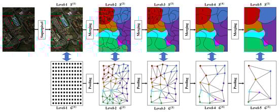
Figure 2.
Progressive merging of superpixels and evolution of graph structure, where the top half is the superpixel merging process. Different colors represent different classes. We take the red region as an example to encode the superpixels and intuitively show the process of superpixel merging. Correspondingly, the bottom half is the graph structure evolution process inspired by the idea of superpixel merging.
Specifically, the pooling process involves merging several graph nodes in graph with merging probability to construct a new graph structure . The process of graph pooling lacks a definite evolutionary path, making it extremely challenging to enumerate all possible evolutionary graphs for evaluation. Hence, we employ a random mechanism to discover an optimal graph pooling result. The graph evolution process of our spatial convolution module is shown in Figure 3.
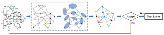
Figure 3.
Illustration of the spatial pooling process. Given the calculated probabilities for merging nodes, the space pooling process involves multiple attempts to merge nodes and generate a new graph until an accepted graph is obtained. The generation of a new graph entails randomly merging some nodes with high merging probability, resulting in the creation of new edges.
First, we randomly select N edges. The edge elimination probability (EEP) between node i and node j can be calculated by
where we define the EEP of nodes with the same label as 1 and the EEP of nodes with different labels as the similarity of two nodes, which can be calculated by Formula (6). Further, the merging probability (MP) of the whole graph can be obtained as
This random merging method can also effectively avoid getting trapped in a local optimum. To evaluate the evolution between two graphs, we define the acceptance probability (AP) from graph to graph as
where is the merging dynamic coefficient, and and denote the posterior probabilities of the graph structures and , respectively. The dynamic coefficient can play a certain supervision role in the spatial pooling process and promote the evolution of a more accurate graph structure. To save time, cost, and computing resources and to ensure efficient completion of the exploration of pooling nodes, we can empirically set the upper bound of the sampling trials, for example, 20 in our experiment. After eliminating the edges with the above determination, the operations of pooling and unpooling can be further defined. First, we define as an evolutionary matrix between and , computed as
Since node information is merged in the process of space pooling, the normalized association matrix is defined as
Next, the spatial pooling function can be denoted as
The unpooling function is expressed as
As shown in Figure 1, after multiple convolution-pooling modules, the final output passes through a fully connected layer with the softmax classifier to obtain the final classification result:
where is the classification result matrix. To optimize the proposed SPGAU, we use the cross-entropy loss function as
where denotes the index set of labeled pixels, C represents the number of classes, and represents the label matrix. Similarly to [59], our network parameters are acquired through training by the Adam optimizer.
4. Experiments
This section summarizes three publicly available HSI datasets to validate the effectiveness of the proposed SPGAU. Then, the experimental settings are introduced. SPGAU was compared to seven effective HSI classification approaches: 3-D CNN [60], GCN [46], MDGCN [61], SSRN [62], SSGCN [63], HybridSN [64], and SVM [9]. Finally, the classification performance was evaluated using metrics such as the overall accuracy (OA), the average accuracy (AA), and the Kappa statistic (Kapp).
4.1. Dataset Description
Three HSI classification datasets were selected for our experiments: the Indian Pines dataset (IP) [60], the Pavia University dataset (PU) [65], and the WHU-HiLongKou dataset (WHU) [66]. We summarize the datasets in Table 1. Specifically, Table 2, Table 3 and Table 4 show the number of training and testing samples for each class of the three datasets, respectively.

Table 1.
Details of the three HSI classification datasets used for experiments.
Table 2.
Category information of the Indian Pines dataset.
Table 3.
Category information of the Pavia University dataset.
Table 4.
Category information of the WHU-Hi-LongKou dataset.
4.2. Experimental Settings
As illustrated in Section 3, the initial level of superpixel segmentation involves image convolutions, while graph convolutions are implemented in subsequent levels. The learning rate is set to with 500 epochs, and the graph depth is 5. Specifically, Table 5 describes the details of SPGAU’s network configuration. The experiments are conducted on a computer equipped with a Nvidia GeForce GTX 2080Ti 11G GPU and an i9-10900K CPU, boasting 64 GB of memory (NVIDIA, Santa Clara, CA, USA). The software environment comprises Python 3.8.5 and PyTorch 1.7.1.
Table 5.
Network configuration of the SPGAU.
4.3. Classification Results
We employed three widely recognized datasets to evaluate the research methods for HSI classification performance. We compared SPGAU with seven HSI classification methods across these benchmark datasets. We set each experiment to be repeated ten times and report the mean and standard deviation for each metric. Table 6, Table 7 and Table 8 present the per-class accuracy, OA, AA, and Kappa coefficients obtained by eight methods on the three datasets, highlighting the best results in bold. Figure 4, Figure 5 and Figure 6 illustrate the HSI classification results obtained by these methods.
Table 6.
Comparison results on the Indian Pines d.
Table 7.
Comparison results on the Pavia University dataset.
Table 8.
Comparison results on the WHU-Hi-LongKou dataset.
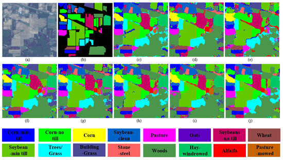
Figure 4.
Classification maps obtained by eight different methods on the Indian Pines dataset. (a) False-color image. (b) Ground-truth map. (c) 3-DCNN. (d) GCN. (e) MDGCN. (f) SSRN. (g) SSGCN. (h) HybridSN. (i) SVM. (j) SPGAU.
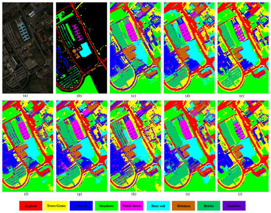
Figure 5.
Classification maps obtained by eight different methods on the Pavia University dataset. (a) False-color image. (b) Ground-truth map. (c) 3-DCNN. (d) GCN. (e) MDGCN. (f) SSRN. (g) SSGCN. (h) HybridSN. (i) SVM. (j) SPGAU.
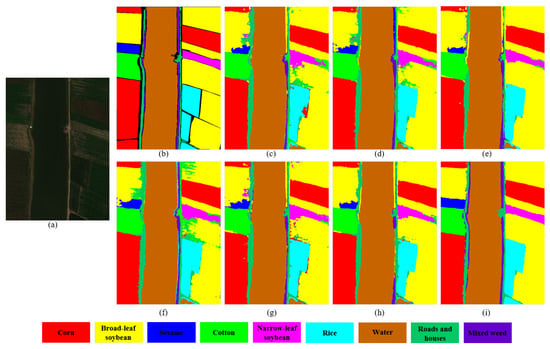
Figure 6.
Classification maps obtained by seven different methods on the WHU-Hi-LongKou dataset. (a) False-color image. (b) Ground-truth map. (c) 3-DCNN. (d) GCN. (e) SSRN. (f) SSGCN. (g) HybridSN. (h) SVM. (i) SPGAU.
Among the various network models, our proposed SPGAU emerges as the top-performing method across all three datasets. Notably, the accuracy for all classes exceeds 90%, with most being optimal. Particularly on the IP and WHU datasets, SPGAU attains an OA, AA, and Kappa coefficient each exceeding 98%. As Table 7 reveals, CNN-based methods outperform GCN-based approaches. Compared with 3D-CNN, SSRN, featuring the residual module, improves OA by 3.06%, while HybridSN achieves an impressive OA of 96%, attributed to its attention mechanism. However, not all GCN-based methods perform poorly. As depicted in Table 7, MDGCN also demonstrates substantial promise, with an OA of 95.24%, positioning it as the second-best performer, just behind SPGAU. The incorporation of multi-scale graph concepts in both SPGAU and MDGCN underscores the importance of multi-scale feature extraction for learning additional spatial features from HSI data. Moreover, because of the relatively large size of the WHU-Hi-LongKou dataset, MDGCN faces challenges in scaling to such data, which is why it is not included in the comparison presented in Table 7. Further insights from the experimental results of SVM in Table 6, Table 7 and Table 8 indicate that machine learning methods can achieve the performance of the deep learning methods. It is worth noting that in Table 6, SVM achieves the optimal accuracy in four categories, second only to the 6-item optimality achieved by our method. However, because the classification accuracy of “Corn-mintill” and “Soybean-mintill” of SVM is less than 80%, the OA of SVM is only 88.59%, which is nearly 10% lower than the 98.56% of SPGAU. This not only affects OA, but the poor Kappa coefficient also reflects the weak spatial consistency between the prediction results of SVM and the actual situation. From the perspective of the classification results in Figure 4, Figure 5 and Figure 6, SPGAU’s classification maps exhibit smoother visual effects with fewer classification errors. For instance, consider the red box section in Figure 4, where “Soybean-min-till” and “Corn-no-till” share similar spectral characteristics. This results in some pixels from “Soybean-min-till” being misclassified as “Corn-no-till” across all classification maps. Additionally, CNN-based methods produce pepper-like errors in certain regions, owing to the absence of spatial context information. In comparison, the classification maps generated by MDGCN and SPGAU, which leverage global information, exhibit stronger spatial correlations. In summary, SPGAU significantly outperforms other algorithms across the three datasets, owing to two key factors as follows:
- 1.
- Attention Mechanism Module: Adding the attention mechanism to graph convolution improves the efficiency of feature aggregation.
- 2.
- Spatial Pooling Module: The spatial pooling module combines similar nodes to generate graph structures at different levels. Building upon this foundation, it extracts more comprehensive global spatial context and spatial details by learning feature information at various scales.
These two modules enrich the feature space from both local and global perspectives, yielding multi-scale features that are well-suited for diverse land cover types. Consequently, SPGAU achieves classification results that are remarkably consistent with the ground truth labels.
5. Discussion
In this section, we first discuss the influence of network depth on the proposed SPGAU, then analyze whether the classification performance of SPGAU is competitive with different numbers of labeled samples, and finally, we briefly compare and analyze the computational efficiency of SPGAU.
5.1. Influence of Network Depth
Graph convolutional networks typically employ no more than three layers to prevent over-smoothing. Our SPGAU overcomes this limitation by incorporating a spatial pooling module, allowing for increased network depth and simplified spatial topology. This enhancement forms a strong basis for extracting deep feature information. To evaluate the impact of network depth on SPGAU’s classification performance, we select network depths ranging from 1 to 6 for the experiments. As depicted in Figure 7, increasing the network depth leads to improved classification accuracy, particularly when the depth reaches 2. This suggests that combining graph convolution with image convolution effectively enhances overall performance. On the PU and WHU datasets, deeper SPGAU leads to improved classification performance. However, for the Pavia University dataset, minimal improvement is observed beyond a depth of 2, mainly due to the presence of discontinuous and fragmented land covers, which limits the efficacy of advanced graph structures.
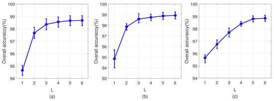
Figure 7.
Classification accuracies of SPAGUN with different network depths. (a) Indian Pines. (b) Pavia University. (c) WHU-Hi-LongKou.
Beyond a network depth of five layers, the improvements in network classification performance become statistically insignificant, leading to the conclusion that the optimal number of network layers is five.
5.2. Impact of the Number of Labeled Examples
Given the high pixel resolution of HSI, manual annotation imposes substantial costs. In this experiment, we examine whether SPGAU maintains a robust classification capability with limited samples. Specifically, we set the training sample proportion for the IP dataset at between 1% and 6% per class and for the PU and WHU datasets at between 0.1% and 0.6% per class. Each experiment is repeated 10 times, and we employ the average OA index to assess the performance of both our proposed SPGAU and the comparative algorithm. The experimental results for the three datasets are presented in Figure 8.
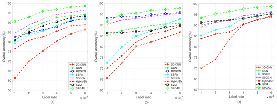
Figure 8.
The classification performance of various methods with different training set ratios on three datasets. (a) Indian Pines. (b) Pavia University. (c) WHU-Hi-LongKou.
Our SPGAU algorithm attains the highest OAs across all datasets. We notice an improvement in OA as the number of labeled instances increases. This suggests that incorporating more labeled data allows the model to acquire more practical information and enhances its training effectiveness. While the GCN-based method outperforms other models in the initial training stage, its OA does not rise significantly with the increase in samples in the later stage. Conversely, although the CNN-based methods exhibit lower OAs with fewer training samples, they consistently exhibit a growth trend over time. This phenomenon underscores the distinct learning characteristics between these two models. By combining their strengths, our SPGAU model achieves superior classification performance, further validating its effectiveness. HybridSN, an attention mechanism-based method, witnesses a significant increase in OAs with increase in the label proportion.
However, it does not reach the level of other methods, indicating that this method may not be suitable for scenarios with a few labeled samples. The MDGCN model secures the second-highest classification accuracy on both the IP and PU datasets. This can be attributed to its multi-scale mechanism, allowing it to learn diverse and informative features, demonstrating adaptability even with the limited labeled samples. Similarly, our SPGAU model, designed as a multi-scale feature extraction and fusion approach, highlights that incorporating diverse models and employing a multi-scale structure can enhance the effectiveness and robustness of HSI classification.
5.3. Running Time
We evaluated the model’s time efficiency, a critical indicator for evaluating the algorithm’s practicality. The experimental settings align with those outlined in Section 4.2. Table 9 reports the time cost (training and testing) of SPGAU on the three datasets. Specifically, machine learning-based SVM exhibits a characteristic of rapid training but slower testing, possibly attributed to the absence of a network structure suitable for GPU acceleration. CNNs are limited by their extensive parameter count, leading to significant time consumption. Notably, for CNN-based deep learning methods, network depth primarily influences processing speed. For instance, SSRN, an extension of the 3D-CNN model incorporating residual modules, results in more layers and longer training and testing times compared to 3D-CNN. Conversely, GCN-based methods do not exhibit an increase in time consumption with larger dataset scales. Interestingly, our proposed SPGAU shows higher time consumption than GCN and SSGCN on the Indian Pines dataset. Nevertheless, SPGAU delivers significantly improved classification performance compared to these two methods. In addition, on large-scale datasets, such as the PU dataset, SPGAU requires less time than GCN and SSGCN while achieving satisfactory results. Thus, our proposed spatial pooling module and graph attention convolution module effectively reduce redundant computations. Given that superpixel preprocessing substantially reduces the graph’s size, SPGAU performs efficiently in terms of time consumption on large-scale datasets. In sum, our proposed SPGAU employs superpixel preprocessing technology to control the graph’s scale, effectively reducing computational complexity.
Table 9.
Comparison of running time between different methods.
6. Conclusions
In this article, we established a novel SPGAU for HSI classification. Unlike conventional GCN models that operate on fixed graphs, SPGAU generates multi-scale graphs by iteratively merging adjacent and similar nodes in the graph. This progressive fusion of features of different scales, from rough to fine, enables the generation of more refined fusion features tailored to HSI classification tasks. Our spatial pooling method facilitates obtaining diverse scale graph structures through the merging of similar and adjacent graph nodes. This operation serves as subsampling, reducing computational complexity while acquiring abstract high-level graph structures. Subsequently, we employed a graph convolution operation with an attention mechanism to enhance the model’s learning capability. The experimental results obtained on three extensively used HSI datasets indicated that SPGAU performs well on small sample experiments in addition to its superior classification performance. Moreover, our method balances the classification accuracy well with the running time. While our method has achieved promising results in HSI classification, the network training process utilized a single-scene HSI dataset, without attempting more complex cross-scene HSI classification research. In future research, we will focus on dynamic graphs and explore the fusion of GNNs with transfer models to cope with cross-scene HSI classification.
Author Contributions
Methodology, Q.D.; conceptualization, Y.D.; formal analysis, Q.D. and X.F.; software, Q.D.; validation, J.W. and Q.D.; writing—original draft preparation, Q.D.; writing—review and editing, C.Z. and Y.D.; supervision, C.Z. and F.P.; project administration, F.P. and X.F.; funding acquisition, F.P. All authors have read and agreed to the published version of the manuscript.
Funding
This research was supported in part by the National Natural Science Foundation of China under Grant 62261160575, Grant 61991414, and Grant 61973036; and in part by the Technical Field Foundation of the National Defense Science and Technology 173 Program under Grant 20220601053, Grant 20220601030.
Data Availability Statement
In this paper, three public hyperspectral datasets are selected. The Indian Pines dataset and the Pavia University dataset are available at http://www.ehu.eus/ccwintco/index.php/HyperspectralRemoteSensingScenes. accessed on 2 August 2022. The WHU-Hi-LongKou dataset is available at http://rsidea.whu.edu.cn/resource_WHUHi_sharing.htm, accessed on 2 August 2022.
Acknowledgments
The authors would like to thank Grupo de Inteligencia Computacional (GIC) and Intelligent Data Extraction, Analysis and Applications of Remote Sensing (RSIDEA). These two organizations have made many excellent hyperspectral datasets publicly available, which provided a lot of choices for our study. We would also like to thank the editors and reviewers for their valuable comments and help with this article.
Conflicts of Interest
The authors declare no conflicts of interest.
References
- Hu, H.; Yao, M.; He, F.; Zhang, F. Graph neural network via edge convolution for hyperspectral image classification. IEEE Geosci. Remote Sens. Lett. 2021, 19, 1–5. [Google Scholar] [CrossRef]
- Sun, L.; Zhao, G.; Zheng, Y.; Wu, Z. Spectral-spatial feature tokenization transformer for hyperspectral image classification. IEEE Trans. Geosci. Remote Sens. 2022, 60, 1–14. [Google Scholar] [CrossRef]
- Ma, X.; Wang, H.; Wang, J. Semisupervised classification for hyperspectral image based on multi-decision labeling and deep feature learning. ISPRS J. Photogramm. Remote Sens. 2016, 120, 99–107. [Google Scholar] [CrossRef]
- Yang, G.; Huang, K.; Sun, W.; Meng, X.; Mao, D.; Ge, Y. Enhanced mangrove vegetation index based on hyperspectral images for mapping mangrove. ISPRS J. Photogramm. Remote Sens. 2022, 189, 236–254. [Google Scholar] [CrossRef]
- Shitharth, S.; Manoharan, H.; Alshareef, A.M.; Yafoz, A.; Alkhiri, H.; Mirza, O.M. Hyper spectral image classifications for monitoring harvests in agriculture using fly optimization algorithm. Comput. Electr. Eng. 2022, 103, 108400. [Google Scholar]
- Shimoni, M.; Haelterman, R.; Perneel, C. Hypersectral imaging for military and security applications: Combining myriad processing and sensing techniques. IEEE Geosci. Remote Sens. Mag. 2019, 7, 101–117. [Google Scholar] [CrossRef]
- Bai, J.; Huang, S.; Xiao, Z.; Li, X.; Zhu, Y.; Regan, A.C.; Jiao, L. Few-shot hyperspectral image classification based on adaptive subspaces and feature transformation. IEEE Trans. Geosci. Remote Sens. 2022, 60, 1–17. [Google Scholar] [CrossRef]
- Rasti, B.; Hong, D.; Hang, R.; Ghamisi, P.; Kang, X.; Chanussot, J.; Benediktsson, J.A. Feature extraction for hyperspectral imagery: The evolution from shallow to deep: Overview and toolbox. IEEE Geosci. Remote Sens. Mag. 2020, 8, 60–88. [Google Scholar] [CrossRef]
- Bo, C.; Lu, H.; Wang, D. Hyperspectral image classification via JCR and SVM models with decision fusion. IEEE Geosci. Remote Sens. Lett. 2015, 13, 177–181. [Google Scholar]
- Li, J.; Bioucas-Dias, J.M.; Plaza, A. Semisupervised hyperspectral image segmentation using multinomial logistic regression with active learning. IEEE Trans. Geosci. Remote Sens. 2010, 48, 4085–4098. [Google Scholar] [CrossRef]
- Bandos, T.V.; Bruzzone, L.; Camps-Valls, G. Classification of hyperspectral images with regularized linear discriminant analysis. IEEE Trans. Geosci. Remote Sens. 2009, 47, 862–873. [Google Scholar] [CrossRef]
- Rodarmel, C.; Shan, J. Principal component analysis for hyperspectral image classification. Surv. Land Inform. Sci. 2002, 62, 115–122. [Google Scholar]
- Zhang, Y.; Ma, Y.; Dai, X.; Li, H.; Mei, X.; Ma, J. Locality-constrained sparse representation for hyperspectral image classification. Inform. Sci. 2021, 546, 858–870. [Google Scholar] [CrossRef]
- Ghamisi, P.; Benediktsson, J.A.; Ulfarsson, M.O. Spectral-spatial classification of hyperspectral images based on hidden Markov random fields. IEEE Trans. Geosci. Remote Sens. 2013, 52, 2565–2574. [Google Scholar] [CrossRef]
- Ye, Z.; Prasad, S.; Li, W.; Fowler, J.E.; He, M. Classification based on 3-D DWT and decision fusion for hyperspectral image analysis. IEEE Geosci. Remote Sens. Lett. 2013, 11, 173–177. [Google Scholar] [CrossRef]
- Jia, S.; Zhuang, J.; Deng, L.; Zhu, J.; Xu, M.; Zhou, J.; Jia, X. 3-D Gaussian-Gabor feature extraction and selection for hyperspectral imagery classification. IEEE Trans. Geosci. Remote Sens. 2019, 57, 8813–8826. [Google Scholar] [CrossRef]
- Fauvel, M.; Benediktsson, J.A.; Chanussot, J.; Sveinsson, J.R. Spectral and spatial classification of hyperspectral data using SVMs and morphological profiles. IEEE Trans. Geosci. Remote Sens. 2008, 46, 3804–3814. [Google Scholar] [CrossRef]
- Fang, L.; He, N.; Li, S.; Ghamisi, P.; Benediktsson, J.A. Extinction profiles fusion for hyperspectral images classification. IEEE Trans. Geosci. Remote Sens. 2017, 56, 1803–1815. [Google Scholar] [CrossRef]
- Huang, H.; Shi, G.; He, H.; Duan, Y.; Luo, F. Dimensionality reduction of hyperspectral imagery based on spatial-spectral manifold learning. IEEE Trans. Cybern. 2019, 50, 2604–2616. [Google Scholar] [CrossRef] [PubMed]
- Fang, L.; Li, S.; Kang, X.; Benediktsson, J.A. Spectral-spatial classification of hyperspectral images with a superpixel-based discriminative sparse model. IEEE Trans. Geosci. Remote Sens. 2015, 53, 4186–4201. [Google Scholar] [CrossRef]
- Ma, L.; Crawford, M.M.; Yang, X.; Guo, Y. Local-manifold-learning-based graph construction for semisupervised hyperspectral image classification. IEEE Trans. Geosci. Remote Sens. 2014, 53, 2832–2844. [Google Scholar] [CrossRef]
- Hong, D.; Gao, L.; Yokoya, N.; Yao, J.; Chanussot, J.; Du, Q.; Zhang, B. More diverse means better: Multimodal deep learning meets remote-sensing imagery classification. IEEE Trans. Geosci. Remote Sens. 2020, 59, 4340–4354. [Google Scholar] [CrossRef]
- Fu, J.; Li, F.; Zhao, J. Real-Time Infrared Horizon Detection in Maritime and Land Environments Based on Hyper-Laplace Filter and Convolutional Neural Network. IEEE Trans. Instrum. Meas. 2023, 72, 1–13. [Google Scholar] [CrossRef]
- Aralikatti, R.C.; Pawan, S.; Rajan, J. A Dual-Stage Semi-Supervised Pre-Training Approach for Medical Image Segmentation. IEEE Trans. Artif. Intell. 2023, 5, 556–565. [Google Scholar] [CrossRef]
- Zhang, Y.; Xu, S.; Hong, D.; Gao, H.; Zhang, C.; Bi, M.; Li, C. Multimodal Transformer Network for Hyperspectral and LiDAR Classification. IEEE Trans. Geosci. Remote Sens. 2023, 61, 1–17. [Google Scholar] [CrossRef]
- Yang, J.; Du, B.; Zhang, L. Overcoming the Barrier of Incompleteness: A Hyperspectral Image Classification Full Model. IEEE Trans. Neural Netw. Learn. Syst. 2023, 1–15. [Google Scholar] [CrossRef] [PubMed]
- Chen, Y.; Lin, Z.; Zhao, X.; Wang, G.; Gu, Y. Deep learning-based classification of hyperspectral data. Int. J. Appl. Earth Obs. Geoinf. 2014, 7, 2094–2107. [Google Scholar] [CrossRef]
- Dong, Y.; Liu, Q.; Du, B.; Zhang, L. Weighted feature fusion of convolutional neural network and graph attention network for hyperspectral image classification. IEEE Trans. Image Process. 2022, 31, 1559–1572. [Google Scholar] [CrossRef] [PubMed]
- Liang, L.; Zhang, S.; Li, J. Multiscale DenseNet meets with bi-RNN for hyperspectral image classification. Int. J. Appl. Earth Obs. Geoinf. 2022, 15, 5401–5415. [Google Scholar] [CrossRef]
- Sellami, A.; Tabbone, S. Deep neural networks-based relevant latent representation learning for hyperspectral image classification. Pattern Recognit. 2022, 121, 108224. [Google Scholar] [CrossRef]
- Yang, B.; Hu, S.; Guo, Q.; Hong, D. Multisource domain transfer learning based on spectral projections for hyperspectral image classification. Int. J. Appl. Earth Obs. Geoinf. 2022, 15, 3730–3739. [Google Scholar] [CrossRef]
- Li, X.; Cao, Z.; Zhao, L.; Jiang, J. ALPN: Active-learning-based prototypical network for few-shot hyperspectral imagery classification. IEEE Geosci. Remote Sens. Lett. 2021, 19, 1–5. [Google Scholar] [CrossRef]
- Gao, K.; Liu, B.; Yu, X.; Yu, A. Unsupervised meta learning with multiview constraints for hyperspectral image small sample set classification. IEEE Trans. Image Process. 2022, 31, 3449–3462. [Google Scholar] [CrossRef]
- Hu, W.; Huang, Y.; Wei, L.; Zhang, F.; Li, H. Deep convolutional neural networks for hyperspectral image classification. J. Sens. 2015, 2015, 1–12. [Google Scholar] [CrossRef]
- Li, Y.; Zhang, H.; Shen, Q. Spectral-spatial classification of hyperspectral imagery with 3D convolutional neural network. Remote Sens. 2017, 9, 67. [Google Scholar] [CrossRef]
- Yang, J.; Zhao, Y.Q.; Chan, J.C.W. Learning and transferring deep joint spectral–spatial features for hyperspectral classification. IEEE Trans. Geosci. Remote Sens. 2017, 55, 4729–4742. [Google Scholar] [CrossRef]
- Chen, C.; Zhang, J.J.; Zheng, C.H.; Yan, Q.; Xun, L.N. Classification of hyperspectral data using a multi-channel convolutional neural network. In Proceedings of the the 14th International Conference on Intelligent Computing (ICIC), Wuhan, China, 15–18 August 2018; pp. 81–92. [Google Scholar]
- Fang, J.; Zhu, Z.; He, G.; Wang, N.; Cao, X. Spatial-spectral Decoupling Framework for Hyperspectral Image Classification. IEEE Geosci. Remote Sens. Lett. 2023, 20, 1–5. [Google Scholar] [CrossRef]
- Shi, H.; Cao, G.; Zhang, Y.; Ge, Z.; Liu, Y.; Yang, D. F3Net: Fast Fourier Filter Network for Hyperspectral Image Classification. IEEE Trans. Instrum. Meas. 2023, 72, 1–18. [Google Scholar] [CrossRef]
- Liu, Q.; Xiao, L.; Yang, J.; Wei, Z. Multilevel superpixel structured graph U-Nets for hyperspectral image classification. IEEE Trans. Geosci. Remote Sens. 2021, 60, 1–15. [Google Scholar] [CrossRef]
- Mou, L.; Lu, X.; Li, X.; Zhu, X.X. Nonlocal graph convolutional networks for hyperspectral image classification. IEEE Trans. Geosci. Remote Sens. 2020, 58, 8246–8257. [Google Scholar] [CrossRef]
- Hong, D.; Gao, L.; Yao, J.; Zhang, B.; Plaza, A.; Chanussot, J. Graph convolutional networks for hyperspectral image classification. IEEE Trans. Geosci. Remote Sens. 2020, 59, 5966–5978. [Google Scholar] [CrossRef]
- Ren, S.; Zhou, F. Semi-supervised classification for PolSAR data with multi-scale evolving weighted graph convolutional network. Int. J. Appl. Earth Obs. Geoinf. 2021, 14, 2911–2927. [Google Scholar] [CrossRef]
- Liu, Q.; Xiao, L.; Yang, J.; Wei, Z. CNN-enhanced graph convolutional network with pixel-and superpixel-level feature fusion for hyperspectral image classification. IEEE Trans. Geosci. Remote Sens. 2020, 59, 8657–8671. [Google Scholar] [CrossRef]
- Defferrard, M.; Bresson, X.; Vandergheynst, P. Convolutional neural networks on graphs with fast localized spectral filtering. Adv. Neural Inf. Process. Syst. 2016, 29, 3844–3852. [Google Scholar]
- Kipf, T.N.; Welling, M. Semi-supervised classification with graph convolutional networks. arXiv 2016, arXiv:1609.02907. [Google Scholar]
- Xu, B.; Shen, H.; Cao, Q.; Qiu, Y.; Cheng, X. Graph wavelet neural network. arXiv 2019, arXiv:1904.07785. [Google Scholar]
- Hechtlinger, Y.; Chakravarti, P.; Qin, J. A generalization of convolutional neural networks to graph-structured data. arXiv 2017, arXiv:1704.08165. [Google Scholar]
- Hamilton, W.; Ying, Z.; Leskovec, J. Inductive representation learning on large graphs. Adv. Neural Inf. Process. Syst. 2017, 30, 1–11. [Google Scholar]
- Velickovic, P.; Cucurull, G.; Casanova, A.; Romero, A.; Lio, P.; Bengio, Y. Graph attention networks. arXiv 2017, arXiv:1710.10903. [Google Scholar]
- Li, Z.P.; Su, H.L.; Zhu, X.B.; Wei, X.M.; Jiang, X.S.; Gribova, V.; Filaretov, V.F.; Huang, D.S. Hierarchical graph pooling with self-adaptive cluster aggregation. IEEE Trans. Cogn. Dev. Syst. 2021, 14, 1198–1207. [Google Scholar] [CrossRef]
- Lee, J.; Lee, I.; Kang, J. Self-attention graph pooling. In Proceedings of the the 36th International Conference on Machine Learning (ICML), Long Beach, CA, USA, 9–15 June 2019; pp. 3734–3743. [Google Scholar]
- Zhang, M.; Cui, Z.; Neumann, M.; Chen, Y. An end-to-end deep learning architecture for graph classification. In Proceedings of the the 32th AAAI Conference on Artificial Intelligence (AAAI-18), New Orleans, LA, USA, 2–7 February 2018; Volume 32, pp. 1–5. [Google Scholar]
- Yuan, H.; Ji, S. Structpool: Structured graph pooling via conditional random fields. In Proceedings of the the 8th International Conference on Learning Representations (ICLR), Addis Ababa, Ethiopia, 26–30 April 2020; pp. 1–12. [Google Scholar]
- Ranjan, E.; Sanyal, S.; Talukdar, P. Asap: Adaptive structure aware pooling for learning hierarchical graph representations. In Proceedings of the the 34th AAAI Conference on Artificial Intelligence (AAAI-20), New York, NY, USA, 7–12 February 2020; Volume 34, pp. 5470–5477. [Google Scholar]
- Achanta, R.; Shaji, A.; Smith, K.; Lucchi, A.; Fua, P.; Susstrunk, S. SLIC superpixels compared to state-of-the-art superpixel methods. IEEE Trans. Pattern Anal. Mach. Intell. 2012, 34, 2274–2282. [Google Scholar] [CrossRef] [PubMed]
- Gao, H.; Ji, S. Graph u-nets. In Proceedings of the the 36th International Conference on Machine Learning (ICML), Long Beach, CA, USA, 9–15 June 2019; pp. 2083–2092. [Google Scholar]
- Maas, A.L.; Hannun, A.Y.; Ng, A.Y. Rectifier nonlinearities improve neural network acoustic models. In Proceedings of the the 30th International Conference on Machine Learning (ICML), Atlanta, GA, USA, 16–21 June 2013; Volume 30, p. 3. [Google Scholar]
- Kingma, D.P.; Ba, J. Adam: A method for stochastic optimization. arXiv 2014, arXiv:1412.6980. [Google Scholar]
- Chen, Y.; Jiang, H.; Li, C.; Jia, X.; Ghamisi, P. Deep feature extraction and classification of hyperspectral images based on convolutional neural networks. IEEE Trans. Geosci. Remote Sens. 2016, 54, 6232–6251. [Google Scholar] [CrossRef]
- Wan, S.; Gong, C.; Zhong, P.; Du, B.; Zhang, L.; Yang, J. Multiscale dynamic graph convolutional network for hyperspectral image classification. IEEE Trans. Geosci. Remote Sens. 2019, 58, 3162–3177. [Google Scholar] [CrossRef]
- Zhong, Z.; Li, J.; Luo, Z.; Chapman, M. Spectral-spatial residual network for hyperspectral image classification: A 3-D deep learning framework. IEEE Trans. Geosci. Remote Sens. 2017, 56, 847–858. [Google Scholar] [CrossRef]
- Qin, A.; Shang, Z.; Tian, J.; Wang, Y.; Zhang, T.; Tang, Y.Y. Spectral-spatial graph convolutional networks for semisupervised hyperspectral image classification. IEEE Geosci. Remote Sens. Lett. 2018, 16, 241–245. [Google Scholar] [CrossRef]
- Roy, S.K.; Krishna, G.; Dubey, S.R.; Chaudhuri, B.B. HybridSN: Exploring 3D-2D CNN feature hierarchy for hyperspectral image classification. IEEE Geosci. Remote Sens. Lett. 2019, 17, 277–281. [Google Scholar] [CrossRef]
- Wang, Z.; Du, B.; Guo, Y. Domain adaptation with neural embedding matching. IEEE Trans. Neural Netw. Learn. Syst. 2019, 31, 2387–2397. [Google Scholar] [CrossRef]
- Zhong, Y.; Hu, X.; Luo, C.; Wang, X.; Zhao, J.; Zhang, L. WHU-Hi: UAV-borne hyperspectral with high spatial resolution (H2) benchmark datasets and classifier for precise crop identification based on deep convolutional neural network with CRF. Remote Sens. Environ. 2020, 250, 112012. [Google Scholar] [CrossRef]
Disclaimer/Publisher’s Note: The statements, opinions and data contained in all publications are solely those of the individual author(s) and contributor(s) and not of MDPI and/or the editor(s). MDPI and/or the editor(s) disclaim responsibility for any injury to people or property resulting from any ideas, methods, instructions or products referred to in the content. |
© 2024 by the authors. Licensee MDPI, Basel, Switzerland. This article is an open access article distributed under the terms and conditions of the Creative Commons Attribution (CC BY) license (https://creativecommons.org/licenses/by/4.0/).