A Unitary Transformation Extension of PolSAR Four-Component Target Decomposition

Abstract

As an improvement on the traditional model-based Yamaguchi four-component decomposition method, in recent years, to fully utilize the polarization information in the coherency matrix, four-component target decomposition methods Y4R and S4R have been proposed, which are based on the rotation of the coherency matrix and the expansion of the volume model, respectively. At the same time, there is also an improved G4U method proposed based on Y4R and S4R. Although these methods have achieved certain decomposition results, there are still problems with overestimation of volume scattering and insufficient utilization of polarization information. In this paper, a unitary transformation extension to the four-component target decomposition method of PolSAR based on the properties of the Jacobi method is proposed. By analyzing the terms in the basic scattering models, such as volume scattering, in the existing four-component decomposition methods, it is clear that the reason for the existence of the residual matrix in the existing decomposition methods is that the off-diagonal term $T_{13}$ and the real part of $T_{23}$ of the coherency matrix $\left[T\right]$ do not participate in the four-component decomposition. On this basis, a matrix transformation method is proposed to decouple terms $T_{13}$ and $\mathrm{Re}\left(T_{23}\right)$, and the residual matrix decomposed based on this method is derived. The performance of the proposed method was validated and evaluated using two datasets. The experimental results indicate that, compared with model-based methods such as Y4R, S4R and G4U, the proposed method can enhance the contribution of double-bounce scattering and odd-bounce scattering power in urban areas in both sets of data. The computational time of the proposed method is equivalent to Y4R, S4R, etc.

1. Introduction

As an important method for interpreting scattering mechanisms from polarimetric synthetic aperture radar (PolSAR) images, polarimetric incoherent target decomposition has been widely studied [1,2,3,4,5,6,7,8]. Besides, related application achievements have shown good application prospects in fields such as target classification and recognition [9,10,11,12].

Among numerous decomposition methods, model-based decomposition methods have clear physical meanings and are widely used in PolSAR target decomposition. However, their results are influenced by the basic scattering model and target orientation. At the same time, decomposition results often have problems such as overestimation of volume scattering, negative power, and insufficient utilization of polarization information [13,14,15], resulting in room for improvement.

The core of the model-based decomposition method is to decompose the scattering into linear combinations of basic scattering components, such as volume scattering, double-bounce scattering, odd-bounce scattering, etc. By analyzing physical parameters such as the power of each basic scattering component, the scattering mechanism of the target can be interpreted. Three-component and four-component model-based scattering power decomposition are popular model-based decomposition methods.

The primitive three-component decomposition model was proposed by Freeman and Durden [16]. Under the assumption of scattering symmetry, cross-polarized scattering coefficient is not correlated with co-polarized scattering coefficient (i.e., $〈S_{\mathrm{HH}}{S}_{\mathrm{HV}}^{\ast }〉=〈S_{\mathrm{VV}}{S}_{\mathrm{HV}}^{\ast }〉=0$ holds, which means $T_{13}=〈\left(S_{\mathrm{HH}}+S_{\mathrm{VV}}\right)S_{\mathrm{HV}}^{\ast }〉$ and $T_{23}=〈\left(S_{\mathrm{HH}}-S_{\mathrm{VV}}\right)S_{\mathrm{HV}}^{\ast }〉$ terms in the PolSAR coherency matrix $\left[T\right]$ are 0), the coherency matrix of nine parameter variables is reduced to five, and the PolSAR coherency matrix is decomposed into a linear combination of backscattering from volume scattering, double-bounce scattering, and odd-bounce scattering. Due to the assumption that scattering symmetry is not applicable to general scenarios with buildings, etc., in order to make the decomposition method more suitable for more scenarios and increase the number of interpretations of coherency matrix terms, Yamaguchi et al. [17] proposed the four-component decomposition method, which does not require scattering symmetry. On the basis of the three-component decomposition method, helix scattering is added as the basic scattering component, which can increase the number of interpretable terms to six. However, for a coherency matrix with nine free parameters, interpreting only six of the terms does not fully utilize polarization information.

In order to further utilize polarization information, Yamaguchi et al. [3] transformed the real part of the $T_{23}$ term into 0 through deorientation (Y4R). After deorientation processing, the parameters of the coherency matrix were reduced from nine to eight, and then, through four-component decomposition, six of the eight parameters could be solved. At the same time, Sato et al. [18] extended Y4R by expanding the volume scattering model (S4R).

Based on the Y4R and S4R four-component decomposition methods, Singh et al. [4] reduced the real and imaginary parts of the $T_{23}$ term to 0 and the parameter variables from eight to seven through further unitary transformation, at the same time, the influence of the $T_{13}$ term was taken into account during the decomposition process and further utilized polarization information (G4U) [4].

In recent years, in order to fully utilize the polarization coherency matrix information, new basic scattering components have been studied. Based on this, optimized polarization decomposition methods such as six-component scattering power decomposition [19] and seven-component scattering power decomposition [7] are proposed. However, although the number of basic scattering models has increased, in some large-azimuth urban areas, the double-bounce scattering component is still not the main scattering mechanism [8]. Maurya et al. [20] optimized the coherency matrix used for decomposition by using selective unitary rotations (Maurya1) and then performed three-component optimization decomposition. Yin et al. [21] added descriptors to urban areas to increase the contribution of double-bounce scattering. While Li et al. [15] proposed the GG4U method on the basis of G4U from a mathematical perspective, this method processes the balance equation system of S4R/Y4R scattering by adding a $T_{13}$ related but redundant balance equation. In this method, Li et al. introduced the decomposition constant $\mu$. When the decomposition constant is $\mu =0$, GG4U changes to S4R, to G4U when $\mu =1$, and to DG4U when $\mu =-1$.

Although the above methods reduce the parameters of the coherency matrix through unitary transformation, the decomposition does not decouple the effects of components that are not involved in the optimization decomposition, i.e., insufficient utilization of polarization information. At the same time, despite the influence of the $T_{13}$ term considered in the GG4U decomposition method, there is always an unknown residual in the GG4U regardless of the unitary transformation used [15].

Ideally, it is essential to completely deorient the PolSAR coherency matrix to decouple the energy that resides in off-diagonal terms in the four-component model-based scattering power decomposition method [20]. This article aims to extend the four-component power decomposition of PolSAR from a mathematical perspective. We focus on decoupling the energy that resides in off-diagonal terms by using the Jacobian method to make the non-diagonal terms of the matrix zero [22]. In addition, three special unitary SU (3) matrices [20] are utilized from the perspective of statistical calculation. The proposed method utilizes the properties of the Jacobi method to perform continuous unitary transformations on the coherency matrix, which effectively decouples the influence of off-diagonal scattering terms on decomposition. The superiority of the newly developed four-component decomposition method was evaluated through the analysis of experimental datasets. Experimental analysis was studied through the total power of cross-polarization, the total power of four scattering mechanisms ($P_{\mathrm{V}}+P_{\mathrm{D}}+P_{\mathrm{S}}+P_{\mathrm{C}}$), helix scattering power ($P_{\mathrm{C}}$), volume scattering power ($P_{\mathrm{V}}$), power of double-bounce scattering and odd-bounce scattering ($P_{\mathrm{D}}+P_{\mathrm{S}}$). These results of different methods along the distance direction and normalized scattering powers mean are compared with the Y4R, S4R and G4U in [3,4,18]. The results of these experiments indicate that the proposed method has an advantage over the Y4R, S4R, and G4U methods in improving the contribution of double-bounce scattering, especially in urban areas.

The organization of this article is as follows: a brief introduction to the PolSAR second-order statistical model is presented in Section 2. Additionally, the Y4R, S4R, and G4U methods and their decomposition residual matrices are presented in Section 3. The principle and flowchart of the proposed method are presented in Section 4, including solutions and a residual matrix. In Section 5, the superiority is validated on different PolSAR datasets by comparing them with Y4R, S4R, and G4U decomposition methods, and Section 6 concludes the paper.

2. PolSAR Coherency Matrix

For a single target in the PolSAR system, the scattering matrix $\left[S\right]$ is:

$$\left[S\right]=\left[\begin{array}{cc}{S}_{\mathrm{HH}}& S_{\mathrm{HV}}\\ S_{\mathrm{VH}}& S_{\mathrm{VV}}\end{array}\right]$$

(1)

where $S_{\mathrm{HH}}, S_{\mathrm{HV}}, S_{\mathrm{VH}}, S_{\mathrm{VV}}$ are the backscatter coefficients of different polarization channels.

With the reciprocal backscattering assumption, the backscatter coefficients in the scattering matrix $\left[S\right]$ meet $S_{\mathrm{HV}}=S_{\mathrm{VH}}$.

Under the Pauli scattering vector ${\mathit{k}}_{\mathrm{P}}$, the coherency matrix can be written as the following $3\times 3$ matrix [3]:

$$\begin{gathered} \left[T\right]=〈{\mathit{k}}_{\mathrm{P}}{\mathit{k}}_{\mathrm{P}}^{\ast \mathrm{T}}〉=\left[\begin{array}{ccc}{T}_{11}& T_{12}& T_{13}\\ T_{21}& T_{22}& T_{23}\\ T_{31}& T_{32}& T_{33}\end{array}\right]=\left[\begin{array}{ccc}{T}_{11}& T_{12}& T_{13}\\ T_{12}^{\ast }& T_{22}& T_{23}\\ T_{13}^{\ast }& T_{23}^{\ast }& T_{33}\end{array}\right], \\ {\mathit{k}}_{\mathrm{P}}=\frac{1}{\sqrt{2}}\left[\begin{array}{c}{S}_{\mathrm{HH}}+S_{\mathrm{VV}}\\ S_{\mathrm{HH}}-S_{\mathrm{VV}}\\ 2S_{\mathrm{HV}}\end{array}\right] \end{gathered}$$

(2)

where the superscript $T$ and $\ast$ stand for the transpose and conjugate operators, respectively, $〈\cdot 〉$ denotes the expectation.

From the expression of (2), the total power (span) of coherency matrices $\left[T\right]$ can be written as:

$$\mathrm{trace}\left(\left[T\right]\right)={\left|S_{\mathrm{HH}}\right|}^2+2{\left|S_{\mathrm{HV}}\right|}^2+{\left|S_{\mathrm{VV}}\right|}^2$$

(3)

3. Y4R, S4R, and G4U PolSAR Decomposition Methods

To reduce the randomness of the target azimuth, the coherency matrix is rotated to reduce the influence of terms in the coherency matrix on PolSAR decomposition. In the unitary transformation-based PolSAR decomposition methods, Y4R and S4R are relatively classic algorithms. Both decomposition methods use volume scattering, double-bounce scattering, odd-bounce scattering, and helix scattering to represent the coherency matrix transformed by the unitary matrix. The expression is as follows:

$$\left[T\prime \right]=P_{\mathrm{V}}\left[T_{\mathrm{V}}\right]+P_{\mathrm{D}}\left[T_{\mathrm{D}}\right]+P_{\mathrm{S}}\left[T_{\mathrm{S}}\right]+P_{\mathrm{C}}\left[T_{\mathrm{C}}\right]$$

(4)

where $\left[T^{\prime }\right]$ is a coherency matrix that undergoes a unitary transformation, which minimizes the cross-polarization power. The conversion is as follows:

$$\left[T\prime \right]=\left[G_{23}\left({\varphi }_1\right)\right]\left[T\right]{\left[G_{23}\left({\varphi }_1\right)\right]}^{-1}=\left(\begin{array}{ccc}{T}_{11}^{\prime }& T_{12}^{\prime }& T_{13}^{\prime }\\ T_{21}^{\prime }& T_{22}^{\prime }& T_{23}^{\prime }\\ T_{31}^{\prime }& T_{32}^{\prime }& T_{33}^{\prime }\end{array}\right)$$

(5)

where $\left[G_{23}\left({\varphi }_1\right)\right]$ is a unitary matrix, and its expression can be found in Equation (2) in [20], $\left[G_{23}\left({\varphi }_1\right)\right]=\left(\begin{array}{ccc}1& 0& 0\\ 0& \cos 2{\varphi }_1& \sin 2{\varphi }_1\\ 0& -\sin 2{\varphi }_1& \cos 2{\varphi }_1\end{array}\right)$, the rotation ${\varphi }_1$ is attained by minimizing the (3, 3) entry of the coherency matrix, ${\varphi }_1=\frac{1}{4}{\tan }^{-1}\left(\frac{2\mathrm{Re}\left(T_{23}\right)}{T_{22}-T_{33}}\right)$.

$\left[T_{\mathrm{V}}\right],\left[T_{\mathrm{D}}\right],\left[T_{\mathrm{S}}\right],\left[T_{\mathrm{C}}\right]$ are the coherency matrices for basic scattering mechanisms such as volume scattering, double-bounce scattering, odd-bounce, and helix scattering, respectively. $P_{\mathrm{V}}, P_{\mathrm{D}}, P_{\mathrm{S}}, P_{\mathrm{C}}$ are the corresponding expansion coefficients. The expressions for $\left[T_{\mathrm{D}}\right]$, $\left[T_{\mathrm{S}}\right]$ and $\left[T_{\mathrm{C}}\right]$ are as follows [4]:

$$\left[T_{\mathrm{D}}\right]=\frac{1}{1+{\left|\alpha \right|}^2}\left[\begin{array}{ccc}{\left|\alpha \right|}^2& \alpha & 0\\ {\alpha }^{\ast }& 1& 0\\ 0& 0& 0\end{array}\right],\left[T_S\right]=\frac{1}{1+{\left|\beta \right|}^2}\left[\begin{array}{ccc}1& {\beta }^{\ast }& 0\\ \beta & {\left|\beta \right|}^2& 0\\ 0& 0& 0\end{array}\right],\left[T_{\mathrm{C}}\right]=\frac{1}{2}\left[\begin{array}{ccc}0& 0& 0\\ 0& 1& \pm j\\ 0& \mathit{\mp }j& 1\end{array}\right]$$

(6)

In (6), $\alpha$ and $\beta$ are the scattering model coefficients of double-bounce scattering and odd-bounce scattering, $j$ is the imaginary unit.

For volume scattering $\left[T_{\mathrm{V}}\right]$, the model can be represented as follows based on the relationship between the backscattering coefficients $S_{\mathrm{HH}}$ and $S_{\mathrm{VV}}$:

$$\left[T_{\mathrm{V}}\right]=\left\{\begin{array}{cccc}\left[T_{\mathrm{V}1}\right],\hfill & \mathrm{Re}\left(S_{\mathrm{HH}}{S}_{\mathrm{VV}}^{\ast }\right)\ge 0\hfill & \mathit{and}\hfill & 10\log \left(\frac{{\left|S_{\mathrm{VV}}\right|}^2}{{\left|S_{\mathrm{HH}}\right|}^2}\right)\le -2\begin{array}{cc}& \end{array}\\ \left[T_{\mathrm{V}2}\right],\hfill & \mathrm{Re}\left(S_{\mathrm{HH}}{S}_{\mathrm{VV}}^{\ast }\right)\ge 0\hfill & \mathit{and}& -2<10\log \left(\frac{{\left|S_{\mathrm{VV}}\right|}^2}{{\left|S_{\mathrm{HH}}\right|}^2}\right)<-2\\ \left[T_{\mathrm{V}3}\right],\hfill & \mathrm{Re}\left(S_{\mathrm{HH}}{S}_{\mathrm{VV}}^{\ast }\right)\ge 0\hfill & \mathit{and}\hfill & 10\log \left(\frac{{\left|S_{\mathrm{VV}}\right|}^2}{{\left|S_{\mathrm{HH}}\right|}^2}\right)\ge 2\begin{array}{cc}& \end{array}\\ \left[T_{\mathrm{V}4}\right],\hfill & \mathrm{Re}\left(S_{\mathrm{HH}}{S}_{\mathrm{VV}}^{\ast }\right)<0\hfill \end{array}\right.$$

(7)

where

$$\left[T_{\mathrm{V}1}\right]=\frac{1}{30}\left[\begin{array}{ccc}15& 5& 0\\ 5& 7& 0\\ 0& 0& 8\end{array}\right],\left[T_{\mathrm{V}2}\right]=\frac{1}{4}\left[\begin{array}{ccc}2& 0& 0\\ 0& 1& 0\\ 0& 0& 1\end{array}\right],\left[T_{\mathrm{V}3}\right]=\frac{1}{30}\left[\begin{array}{ccc}15& -5& 0\\ -5& 7& 0\\ 0& 0& 8\end{array}\right],\left[T_{\mathrm{V}4}\right]=\frac{1}{15}\left[\begin{array}{ccc}0& 0& 0\\ 0& 7& 0\\ 0& 0& 8\end{array}\right]$$

(8)

There are various volume scattering models in (8), but they can all be written in the following form:

$$\left[T_{\mathrm{V}}\right]=\left[\begin{array}{ccc}a& d& 0\\ d& b& 0\\ 0& 0& c\end{array}\right]$$

(9)

where $a,b,c$ are variables, satisfying $a+b+c=1$, $d$ is a constant.

According to the models of volume scattering, double-bounce scattering, odd-bounce scattering, helix scattering in (6)–(8), and the coherency matrix decomposition expression (4), the residual matrix after Y4R and S4R decomposition can be obtained as [15]:

$$\left[T_{\mathrm{R}}^{\prime }\right]=\left[\begin{array}{ccc}0& 0& T_{13}^{\prime }\\ 0& 0& 0\\ T_{31}^{\prime }& 0& 0\end{array}\right]$$

(10)

From the above equation, it can be seen that after the unitary matrix $\left[G_{23}\left({\varphi }_1\right)\right]$ transformation, there is still the influence of $T{\prime }_{13}$ in the residual matrix. To overcome this problem, the G4U method proposed by Li et al. utilizes $\left[U_{23}\left({\varphi }_2\right)\right]$ to perform a unitary transformation on $\left[T^{\prime }\right]$, that is:

$$\left[T^{″}\right]=\left[U_{23}\left({\varphi }_2\right)\right]\left[T\prime \right]{\left[U_{23}\left({\varphi }_2\right)\right]}^{-1}$$

(11)

where $\left[U_{23}\left({\varphi }_2\right)\right]$ can be found in Equation (9) in [4] and ${\varphi }_2=\frac{1}{4}{\tan }^{-1}\left(\frac{2\mathrm{Im}\left(T_{23}\left({\varphi }_1\right)\right)}{T_{22}\left({\varphi }_1\right)-T_{33}\left({\varphi }_1\right)}\right)$.

Similar to $\left[T_{\mathrm{R}}^{\prime }\right]$ in (14), the residual matrix after G4U decomposition is [15]:

$$\left[T_{\mathrm{R}}^{″}\right]=\left[\begin{array}{ccc}0& -T_{\mathrm{13}}^{\prime }& T_{\mathrm{13}}^{\prime }\\ -T_{\mathrm{31}}^{\prime }& 0& 0\\ T_{\mathrm{31}}^{\prime }& 0& 0\end{array}\right]$$

(12)

In addition to the commonly used four-component decomposition methods mentioned above, in recent years, to overcome the problem of overestimation of volume scattering power, in 2019, Maurya1 method [20] choose the unitary transformation method to minimize the cross-polarization energy. At the same time, An [23] and Maurya [24] (Maurya2) also proposed different hybrid decomposition techniques, incorporating eigenvalue decomposition in model decomposition. These methods determine the maximum possible value of volume scattering power $P_{\mathrm{V}}$ through eigenvalue decomposition [23]:

$$\left[T\right]x=\lambda \left[T_{\mathrm{V}}\right]x$$

(13)

Then, $P_{\mathrm{V}}$ can be determined by solving the following cubic equation:

$$\det \left(\left[T\right]-\lambda \left[T_{\mathrm{V}}\right]\right)=0$$

(14)

From the above equation, three eigenvalues can be obtained, ${\lambda }_1,{\lambda }_2,{\lambda }_3$, then $P_{\mathrm{V}}=\min \left\{{\lambda }_1,{\lambda }_2,{\lambda }_3\right\}$. After deriving $P_{\mathrm{V}}$ and extracting the volume scattering component $P_{\mathrm{V}}\left[T_{\mathrm{V}}\right]$ from the original coherency matrix $\left[T\right]$, the remaining matrix $\left[T_{\mathrm{re}}\right]$, including double-bounce scattering and odd-bounce scattering, can be written as:

$$\left[T_{\mathrm{re}}\right]=\left[T\right]-P_{\mathrm{V}}\left[T_{\mathrm{V}}\right]$$

(15)

The rank of the remaining $\left[T_{\mathrm{re}}\right]$ is at most 2, on this basis, using the method of unitary transformation, An and Maurya2 constructed different models for double-bounce scattering and odd-bounce scattering to obtain their scattering powers.

4. Decomposing Method Based on the Jacobi Method

In the four-component model-based scattering power decomposition method of PolSAR, the basic scattering models such as volume scattering, double-bounce scattering, odd-bounce scattering, and helix scattering do not contain the term $T_{13}$ and the real part of $T_{23}$. Ideally, the measured coherency matrix should be completely reoriented to avoid any ambiguity in the scattering mechanism. However, implementing unitary transformation on the coherency matrix $\left[T\right]$ alone cannot achieve the elimination of the term $T_{13}$ and the real part of $T_{23}$. Therefore, most existing studies decouple the off-diagonal term $T_{13}$ or $T_{23}$ of the PolSAR coherency matrix to minimize the impact of the off-diagonal terms.

This article is from the perspective of statistical calculation and the properties of the Jacobi method to ensure the energy of the coherency matrix so that the coherency matrix used for PolSAR decomposition does not contain the term $T_{13}$ and the real part of $T_{23}$, in order to eliminate the influence of off-diagonal terms on the decomposition.

For real symmetric matrices, the Jacobi method can make any non-diagonal element equal to 0, and all non-diagonal elements can be eliminated through continuous iterations. Furthermore, the energy of the matrix and the sum of squares of all elements remain unchanged after the Jacobi iteration. To this end, the Jacobi method for real symmetric matrices is extended to the complex coherency symmetric matrix $\left[T\right]$ of polarization.

Performing the unitary transformation of the coherency matrix $\left[T\right]$:

$$\left[T^{\left(1\right)}\right]=\left[C_{13}\left(\theta \right)\right]\left[T\right]{\left[C_{13}\left(\theta \right)\right]}^{-1}$$

(16)

where

$$\left[C_{13}\left(\theta \right)\right]=\left[U_{13}\left({\theta }_2\right)\right]\left[G_{13}\left({\theta }_1\right)\right]$$

(17)

$\left[G_{13}\left({\theta }_1\right)\right]$, $\left[U_{13}\left({\theta }_2\right)\right]$ are unitary matrices, ${\theta }_1$ and ${\theta }_2$ are:

$$\begin{gathered} \left[G_{13}\left({\theta }_1\right)\right]=\left(\begin{array}{ccc}\cos 2{\theta }_1& 0& \sin 2{\theta }_1\\ 0& 1& 0\\ -\sin 2{\theta }_1& 0& \cos 2{\theta }_1\end{array}\right), \left[U_{13}\left({\theta }_2\right)\right]=\left(\begin{array}{ccc}\cos 2{\theta }_2& 0& j\sin 2{\theta }_2\\ 0& 1& 0\\ j\sin 2{\theta }_2& 0& \cos 2{\theta }_2\end{array}\right) \\ {\theta }_1=\frac{1}{4}{\tan }^{-1}\left(\frac{2\mathrm{Re}\left(T_{13}\right)}{T_{11}-T_{33}}\right), {\theta }_2=\frac{1}{4}{\tan }^{-1}\left(\frac{2\mathrm{Im}\left(T_{13}\left({\theta }_1\right)\right)}{T_{11}\left({\theta }_1\right)-T_{33}\left({\theta }_1\right)}\right) \end{gathered}$$

(18)

The real part and the imaginary part of the $T_{13}$ term can be removed, respectively through unitary transformation $\left[G_{13}\left({\theta }_1\right)\right]$ and $\left[U_{13}\left({\theta }_2\right)\right]$.

Since $\left[G_{13}\left({\theta }_1\right)\right]$ and $\left[U_{13}\left({\theta }_2\right)\right]$ are unitary matrices, $\left[{\mathrm{C}}_{13}\left(\theta \right)\right]$ remains a unitary matrix.

Thus, the terms in $\left[T^{\left(1\right)}\right]$ can be represented as:

$$\begin{array}{l}{T}_{11}^{\left(1\right)}=T_{11}\left({\theta }_1\right){\cos }^{2}2{\theta }_2+T_{33}\left({\theta }_1\right){\sin }^{2}2{\theta }_2+\mathrm{Im}\left(T_{13}\left({\theta }_1\right)\right)\sin 4{\theta }_2\\ T_{12}^{\left(1\right)}=T_{12}\left({\theta }_1\right)\cos 2{\theta }_2+j{T}_{23}^{\ast }\left({\theta }_1\right)\sin 2{\theta }_2\\ T_{13}^{\left(1\right)}=0\\ T_{21}^{\left(1\right)}={\stackrel{⌢}{T}}_{12}^{\left(1\right)\ast }\\ T_{22}^{\left(1\right)}=T_{22}\\ T_{23}^{\left(1\right)}=T_{23}\left({\theta }_1\right)\cos 2{\theta }_2-j{T}_{12}^{\ast }\left({\theta }_1\right)\sin 2{\theta }_2\\ T_{31}^{\left(1\right)}=T_{13}^{\left(1\right)\ast }=0\\ T_{32}^{\left(1\right)}=T_{23}^{\left(1\right)\ast }\\ T_{33}^{\left(1\right)}=T_{33}\left({\theta }_1\right){\cos }^{2}2{\theta }_2+T_{11}\left({\theta }_1\right){\sin }^{2}2{\theta }_2-\mathrm{Im}\left(T_{13}\left({\theta }_1\right)\right)\sin 4{\theta }_2\end{array}$$

(19)

In the above equation, the expression for $T_{ij}\left({\theta }_1\right)$ is:

$$\begin{array}{l}{T}_{11}\left({\theta }_1\right)=T_{11}{\cos }^{2}2{\theta }_1+T_{33}{\sin }^{2}2{\theta }_1+\mathrm{Re}\left(T_{13}\right)\sin 4{\theta }_1\\ T_{12}\left({\theta }_1\right)=T_{12}\cos 2{\theta }_1+T_{32}\sin 2{\theta }_1\\ T_{13}\left({\theta }_1\right)=j\mathrm{Im}\left(T_{13}\right)\\ T_{22}\left({\theta }_1\right)=T_{22}\\ T_{23}\left({\theta }_1\right)=T_{23}\cos 2{\theta }_1-T_{21}\sin 2{\theta }_1\\ T_{33}\left({\theta }_1\right)=T_{33}{\cos }^{2}2{\theta }_1+T_{11}{\sin }^{2}2{\theta }_1-\mathrm{Re}\left(T_{13}\right)\sin 4{\theta }_1\end{array}$$

(20)

In particular, if $T_{13}=0$, according to the expression of ${\theta }_1$ and ${\theta }_2$, ${\theta }_1=0$ and ${\theta }_2=0$, furthermore, after transforming in (16), $\left[T^{\left(1\right)}\right]=\left[T\right]$. At the same time, if $T_{13}\ne 0$ and $T_{23}=0$, after transforming $\left[T^{\left(1\right)}\right]=\left[C_{13}\left(\theta \right)\right]\left[T\right]{\left[C_{13}\left(\theta \right)\right]}^{-1}$, $T_{23}$ is no longer 0, but:

$$T_{23}^{\left(1\right)}=-T_{12}^{\ast }\sin 2{\theta }_1\cos 2{\theta }_2-j{T}_{12}^{\ast }\cos 2{\theta }_1\sin 2{\theta }_2$$

(21)

From (16), $T_{13}^{\left(1\right)}=0$. Using $D\left(\left[T\right]\right)$ to represent the sum of squares of diagonal terms in the coherency matrix $\left[T\right]$, then $D\left(\left[T\right]\right)$ can be expressed as:

$$D\left(\left[T\right]\right)={\left|T_{11}\right|}^2+{\left|T_{22}\right|}^2+{\left|T_{33}\right|}^2$$

(22)

At the same time, using $E\left(\left[T\right]\right)$ to represent the sum of squares of off-diagonal terms, then $E\left(\left[T\right]\right)$ can be expressed as:

$$E\left(\left[T\right]\right)={‖\left[T\right]‖}_F^2-D\left(\left[T\right]\right)=2\left({\left|T_{12}\right|}^2+{\left|T_{13}\right|}^2+{\left|T_{23}\right|}^2\right)$$

(23)

where ${‖\left[T\right]‖}_F^2$ represents the square of the F-norm.

Further,

$$\begin{array}{l}{\left|T_{12}^{\left(1\right)}\right|}^2+{\left|T_{13}^{\left(1\right)}\right|}^2+{\left|T_{23}^{\left(1\right)}\right|}^2\\ ={\left(\mathrm{Re}\left(T_{12}\right)\cos 2{\theta }_1+\mathrm{Re}\left(T_{23}\right)\sin 2{\theta }_1\right)}^2+{\left(\mathrm{Im}\left(T_{12}\right)\cos 2{\theta }_1-\mathrm{Im}\left(T_{23}\right)\sin 2{\theta }_1\right)}^2\\ \begin{array}{cc}& +{\left(\mathrm{Re}\left(T_{23}\right)\cos 2{\theta }_1-\mathrm{Re}\left(T_{12}\right)\sin 2{\theta }_1\right)}^2+{\left(\mathrm{Im}\left(T_{23}\right)\cos 2{\theta }_1+\mathrm{Im}\left(T_{12}\right)\sin 2{\theta }_1\right)}^2\end{array}+0\\ ={\left(\mathrm{Re}\left(T_{12}\right)\right)}^2+{\left(\mathrm{Re}\left(T_{23}\right)\right)}^2+{\left(\mathrm{Im}\left(T_{12}\right)\right)}^2+{\left(\mathrm{Im}\left(T_{23}\right)\right)}^2\\ ={\left|T_{12}\right|}^2+{\left|T_{23}\right|}^2\end{array}$$

(24)

$$\begin{array}{l}E\left(\left[T^{\left(1\right)}\right]\right)=2\left({\left|T_{12}^{\left(1\right)}\right|}^2+{\left|T_{13}^{\left(1\right)}\right|}^2+{\left|T_{23}^{\left(1\right)}\right|}^2\right)\\ =2\left({\left|T_{12}\right|}^2+{\left|T_{23}\right|}^2+0\right)\\ =E\left(\left[T\right]\right)-2{\left|T_{13}\right|}^2\end{array}$$

(25)

Similarly, performing the unitary transformation $\left[{\stackrel{⌢}{T}}^{\left(1\right)}\right]=\left[C_{23}\left(\varphi \right)\right]\left[T^{\left(1\right)}\right]\left[C_{23}{\left(\varphi \right)}^{-1}\right]$, $\left[C_{23}\left(\varphi \right)\right]$ satisfies $\left[C_{23}\left(\varphi \right)\right]=\left[G_{23}\left({\varphi }_1\right)\right]$. $\left[G_{23}\left({\varphi }_1\right)\right]=\left(\begin{array}{ccc}1& 0& 0\\ 0& \cos 2{\varphi }_1& \sin 2{\varphi }_1\\ 0& -\sin 2{\varphi }_1& \cos 2{\varphi }_1\end{array}\right)$ is a unitary matrix and can be found in Equation (2) in [20]. Based on the unitary transformation above, the terms in $\left[{\stackrel{⌢}{T}}^{\left(1\right)}\right]$ can be expressed as:

$$\begin{array}{l}{\stackrel{⌢}{T}}_{11}^{\left(1\right)}=T_{11}^{\left(1\right)}\\ {\stackrel{⌢}{T}}_{12}^{\left(1\right)}=T_{12}^{\left(1\right)}\cos 2{\varphi }_1+T_{13}^{\left(1\right)}\sin 2{\varphi }_1\\ {\stackrel{⌢}{T}}_{13}^{\left(1\right)}=-T_{12}^{\left(1\right)}\sin 2{\varphi }_1+T_{13}^{\left(1\right)}\cos 2{\varphi }_1\\ {\stackrel{⌢}{T}}_{22}^{\left(1\right)}=T_{22}^{\left(1\right)}{\cos }^{2}2{\varphi }_1+T_{33}^{\left(1\right)}{\sin }^{2}2{\varphi }_1+\mathrm{Re}\left(T_{23}^{\left(1\right)}\right)\sin 4{\varphi }_1\\ {\stackrel{⌢}{T}}_{23}^{\left(1\right)}=j\mathrm{Im}\left(T_{23}^{\left(1\right)}\right)\\ {\stackrel{⌢}{T}}_{33}^{\left(1\right)}=T_{22}^{\left(1\right)}{\sin }^{2}2{\varphi }_1+T_{33}^{\left(1\right)}{\cos }^{2}2{\varphi }_1-\mathrm{Re}\left(T_{23}^{\left(1\right)}\right)\sin 4{\varphi }_1\end{array}$$

(26)

$$\begin{array}{cc}\hfill E\left(\left[{\stackrel{⌢}{T}}^{\left(1\right)}\right]\right)& =2\left({\left|{\stackrel{⌢}{T}}_{12}^{\left(1\right)}\right|}^2+{\left|{\stackrel{⌢}{T}}_{13}^{\left(1\right)}\right|}^2+{\left|{\stackrel{⌢}{T}}_{23}^{\left(1\right)}\right|}^2\right)\hfill \\ \hfill & =E\left(\left[T^{\left(1\right)}\right]\right)-2{\left|\mathrm{Re}\left(T_{23}^{\left(1\right)}\right)\right|}^2\hfill \\ \hfill & =E\left(\left[T\right]\right)-2{\left|T_{13}\right|}^2-2{\left|\mathrm{Re}\left(T_{23}^{\left(1\right)}\right)\right|}^2\hfill \end{array}$$

(27)

In particular, if $T_{13}=0$ and $\mathrm{Re}\left(T_{23}\right)=0$, then $\left[T^{\left(1\right)}\right]=\left[T\right]$ and ${\varphi }_1=0$, and further there is:

$$\left[{\stackrel{⌢}{T}}^{\left(1\right)}\right]=\left[T\right]$$

(28)

According to the properties of Jacobi method, generally, let:

$$\left[T^{\left(0\right)}\right]=\left[T\right]$$

(29)

After $n$ iterations, the coherency matrix becomes:

$$\begin{array}{cc}\left[{\stackrel{⌢}{T}}^{\left(n\right)}\right]& =\left[C_{23}\left({\varphi }_n\right)\right]\left[T^{\left(n\right)}\right]{\left[C_{23}\left({\varphi }_n\right)\right]}^{-1}\hfill \\ & =\left[C_{23}\left({\varphi }_n\right)\right]\left[C_{13}\left({\theta }_n\right)\right]\left[{\stackrel{⌢}{T}}^{\left(n-1\right)}\right]\left[C_{13}{\left({\theta }_n\right)}^{-1}\right]{\left[C_{23}\left({\varphi }_n\right)\right]}^{-1}\\ & =\left[G_{23}\left({\varphi }_{n,1}\right)\right]\left[U_{13}\left({\theta }_{n,2}\right)\right]\left[G_{13}\left({\theta }_{n,1}\right)\right]\left[{\stackrel{⌢}{T}}^{\left(n-1\right)}\right]{\left[G_{13}\left({\theta }_{n,1}\right)\right]}^{-1}{\left[U_{13}\left({\theta }_{n,2}\right)\right]}^{-1}{\left[G_{23}\left({\varphi }_{n,1}\right)\right]}^{-1}\hfill \end{array}$$

(30)

where

$${\theta }_{n,1}=\frac{1}{4}\arctan \left(\frac{2\mathrm{Re}\left(T_{13}^{\left(n-1\right)}\right)}{T_{11}^{\left(n-1\right)}-T_{33}^{\left(n-1\right)}}\right),{\theta }_{n,2}=\frac{1}{4}{\tan }^{-1}\left(\frac{2\mathrm{Im}\left\{T_{13}^{\left(n-1\right)}\left({\theta }_{n,1}\right)\right\}}{T_{11}^{\left(n-1\right)}\left({\theta }_{n,1}\right)-T_{33}^{\left(n-1\right)}\left({\theta }_{n,1}\right)}\right)$$

(31)

$${\varphi }_{n,1}=\frac{1}{4}{\tan }^{-1}\left(\frac{2\mathrm{Re}\left\{T_{23}^{\left(n-1\right)}\left({\theta }_{n,2}\right)\right\}}{T_{22}^{\left(n-1\right)}\left({\theta }_{n,2}\right)-T_{33}^{\left(n-1\right)}\left({\theta }_{n,2}\right)}\right)$$

(32)

Then,

$$\begin{array}{l}E\left(\left[T^{\left(n\right)}\right]\right)=E\left(\left[T^{\left(n-1\right)}\right]\right)-2{\left|T_{13}^{\left(n-1\right)}\right|}^2\\ E\left(\left[{\stackrel{⌢}{T}}^{\left(n\right)}\right]\right)=2\left({\left|{\stackrel{⌢}{T}}_{12}^{\left(n\right)}\right|}^2+{\left|{\stackrel{⌢}{T}}_{13}^{\left(n\right)}\right|}^2+{\left|{\stackrel{⌢}{T}}_{23}^{\left(n\right)}\right|}^2\right)=E\left(\left[T^{\left(n\right)}\right]\right)-2{\left|\mathrm{Re}\left(T_{23}^{\left(n\right)}\right)\right|}^2=E\left(\left[T^{\left(n-1\right)}\right]\right)-2{\left|T_{13}^{\left(n-1\right)}\right|}^2-2{\left|\mathrm{Re}\left(T_{23}^{\left(n\right)}\right)\right|}^2\end{array}$$

(33)

In particular, when $n=3$

$$\begin{array}{l}E\left(\left[T^{\left(3\right)}\right]\right)=E\left(\left[T^{\left(2\right)}\right]\right)-2{\left|T_{13}^{\left(2\right)}\right|}^2\\ E\left(\left[{\stackrel{⌢}{T}}^{\left(3\right)}\right]\right)=2\left({\left|{\stackrel{⌢}{T}}_{12}^{\left(3\right)}\right|}^2+{\left|{\stackrel{⌢}{T}}_{13}^{\left(3\right)}\right|}^2+{\left|{\stackrel{⌢}{T}}_{23}^{\left(3\right)}\right|}^2\right)=E\left(\left[T^{\left(3\right)}\right]\right)-2{\left|\mathrm{Re}\left(T_{23}^{\left(3\right)}\right)\right|}^2=E\left(\left[T^{\left(2\right)}\right]\right)-2{\left|T_{13}^{\left(2\right)}\right|}^2-2{\left|\mathrm{Re}\left(T_{23}^{\left(3\right)}\right)\right|}^2\end{array}$$

(34)

From Equation (33), it can be seen that $E\left(\left[{\stackrel{⌢}{T}}^{\left(n\right)}\right]\right)$ monotonically decreases and has a lower bound. In regard to $\left|T_{13}^{\left(n-1\right)}\right|$ and $\left|\mathrm{Re}\left(T_{23}^{\left(n\right)}\right)\right|$, when $E\left(\left[{\stackrel{⌢}{T}}^{\left(n\right)}\right]\right)$ converges to a stable value, it means that $\left|T_{13}^{\left(n-1\right)}\right|$ and $\left|\mathrm{Re}\left(T_{23}^{\left(n\right)}\right)\right|$ no longer change, according to the convergence of Jacobi’s method, thus, $\left|T_{13}^{\left(n-1\right)}\right|$ and $\left|\mathrm{Re}\left(T_{23}^{\left(n\right)}\right)\right|$ satisfy:

$$\begin{array}{l}\underset{n\to \infty }{\lim }{T}_{13}^{\left(n\right)}=0,\\ \underset{n\to \infty }{\lim }\mathrm{Re}\left(T_{23}^{\left(n\right)}\right)=0\end{array}$$

(35)

The $\left[{\stackrel{⌢}{T}}^{\left(n\right)}\right]$ that meets the condition is rewritten as $\left[\stackrel{⌢}{T}\right]$,

$$\left[\stackrel{⌢}{T}\right]=\left[\begin{array}{ccc}{\stackrel{⌢}{T}}_{11}& {\stackrel{⌢}{T}}_{12}& 0\\ {\stackrel{⌢}{T}}_{21}& {\stackrel{⌢}{T}}_{22}& {\stackrel{⌢}{T}}_{23}\\ 0& {\stackrel{⌢}{T}}_{32}& {\stackrel{⌢}{T}}_{33}\end{array}\right]$$

(36)

A special case is if $T_{13}=0$ and $\mathrm{Re}\left(T_{23}\right)=0$, then even after $n$ iterations, $\left[\stackrel{⌢}{T}\right]=\left[T\right]$. In other words, if $\left[\stackrel{⌢}{T}\right]$ satisfies ${\stackrel{⌢}{T}}_{13}=0$ and $\mathrm{Re}\left({\stackrel{⌢}{T}}_{23}\right)=0$ after $n$ iterations, even if the above iteration is continued, the size of the terms in $\left[\stackrel{⌢}{T}\right]$ will not be changed.

According to the above processing, the influence of the term $T_{13}$ and the real part of $T_{23}$ in the original $\left[T\right]$ are decoupled, and all energy in $\left[T\right]$ is concentrated on other components, excluding the term $T_{13}$ and the real part of $T_{23}$. This method comprehensively utilizes scattering information and effectively utilizes all information in the coherency matrix through rotation transformation.

The above transformations are all based on unitary matrix transformations, therefore,

$$\mathrm{Span}=\mathrm{trace}\left(\left[T\right]\right)=\mathrm{trace}\left(\left[\stackrel{⌢}{T}\right]\right)={\stackrel{⌢}{T}}_{11}+{\stackrel{⌢}{T}}_{22}+{\stackrel{⌢}{T}}_{33}$$

(37)

The transformed matrix $\left[\stackrel{⌢}{T}\right]$ is represented as a linear combination of volume scattering, double-bounce scattering, odd-bounce scattering and helix scattering:

$$\left[\stackrel{⌢}{T}\right]=P_{\mathrm{V}}\left[T_{\mathrm{V}}\right]+P_{\mathrm{D}}\left[T_{\mathrm{D}}\right]+P_{\mathrm{S}}\left[T_{\mathrm{S}}\right]+P_{\mathrm{C}}\left[T_{\mathrm{C}}\right]$$

(38)

where $\left[T_{\mathrm{V}}\right],\left[T_{\mathrm{D}}\right],\left[T_{\mathrm{S}}\right],\left[T_{\mathrm{C}}\right]$ are the coherency matrices for basic scattering mechanisms such as volume scattering, double-bounce scattering, odd-bounce scattering, and helix scattering, respectively. The models of $\left[T_{\mathrm{V}}\right],\left[T_{\mathrm{D}}\right],\left[T_{\mathrm{S}}\right],\left[T_{\mathrm{C}}\right]$ can be seen in (6)–(8). $P_{\mathrm{V}},P_{\mathrm{D}},P_{\mathrm{S}},P_{\mathrm{C}}$ are the corresponding expansion coefficients.

The expansion of (38) leads to:

$$\begin{array}{l}{\stackrel{⌢}{T}}_{11}=P_{\mathrm{v}}a+P_{\mathrm{D}}\frac{{\left|\alpha \right|}^2}{1+{\left|\alpha \right|}^2}+P_{\mathrm{S}}\frac{1}{1+{\left|\beta \right|}^2}\\ {\stackrel{⌢}{T}}_{12}=P_{\mathrm{v}}d+P_{\mathrm{D}}\frac{\alpha }{1+{\left|\alpha \right|}^2}+P_{\mathrm{S}}\frac{{\beta }^{\ast }}{1+{\left|\beta \right|}^2}\\ {\stackrel{⌢}{T}}_{22}=P_{\mathrm{v}}b+P_{\mathrm{D}}\frac{1}{1+{\left|\alpha \right|}^2}+P_{\mathrm{S}}\frac{{\left|\beta \right|}^2}{1+{\left|\beta \right|}^2}\\ {\stackrel{⌢}{T}}_{23}=\pm \frac{1}{2}j{P}_{\mathrm{C}}\\ {\stackrel{⌢}{T}}_{33}=P_{\mathrm{v}}c+\frac{1}{2}{P}_{\mathrm{C}}\end{array}$$

(39)

In the above equation, $a,b,c$ and $d$ are the parameters of volume scattering, all of which are constants. $\alpha$ and $\beta$ are the scattering model-coefficients of double-bounce scattering, and odd-bounce scattering. From the above equation, it can be concluded that the expression for $P_{\mathrm{C}}$ is:

$$P_{\mathrm{C}}=2\left|{\stackrel{⌢}{T}}_{23}\right|$$

(40)

After $P_{\mathrm{C}}$ is determined, $P_{\mathrm{V}}$ can be determined based on the size of $\mathrm{Re}\left(S_{\mathrm{HH}}{S}_{\mathrm{VV}}^{\ast }\right)$ and $10\log \left(\frac{{\left|S_{\mathrm{VV}}\right|}^2}{{\left|S_{\mathrm{HH}}\right|}^2}\right)$ after removing the helix scattering from $\left[T^{\prime }\right]$. Let $L_1=\mathrm{Re}\left(S_{\mathrm{HH}}{S}_{\mathrm{VV}}^{\ast }\right)$ and $L_2=10\log \left(\frac{{\left|S_{\mathrm{VV}}\right|}^2}{{\left|S_{\mathrm{HH}}\right|}^2}\right)$, then:

$$\begin{gathered} L_1={\stackrel{⌢}{T}}_{11}-{\stackrel{⌢}{T}}_{22}+\frac{1}{2}{P}_{\mathrm{C}} \\ {L}_2=10\log \left(\frac{{\stackrel{⌢}{T}}_{11}+{\stackrel{⌢}{T}}_{22}-2\mathrm{Re}\left({\stackrel{⌢}{T}}_{12}\right)}{{\stackrel{⌢}{T}}_{11}+{\stackrel{⌢}{T}}_{22}+2\mathrm{Re}\left({\stackrel{⌢}{T}}_{12}\right)}\right) \end{gathered}$$

(41)

According to (39), $P_{\mathrm{V}}$ can be determined:

$$P_{\mathrm{V}}=\frac{1}{c}{\stackrel{⌢}{T}}_{33}-\frac{1}{2c}{P}_{\mathrm{C}}$$

(42)

Furthermore, (39) becomes:

$$\left\{\begin{array}{c}{P}_{\mathrm{D}}\frac{{\left|\alpha \right|}^2}{1+{\left|\alpha \right|}^2}+P_{\mathrm{S}}\frac{1}{1+{\left|\beta \right|}^2}=S\\ P_{\mathrm{D}}\frac{\alpha }{1+{\left|\alpha \right|}^2}+P_{\mathrm{S}}\frac{{\beta }^{\ast }}{1+{\left|\beta \right|}^2}=C\\ P_{\mathrm{D}}\frac{1}{1+{\left|\alpha \right|}^2}+P_{\mathrm{S}}\frac{{\left|\beta \right|}^2}{1+{\left|\beta \right|}^2}=D\end{array}\right.$$

(43)

where

$$\left\{\begin{array}{c}S={\stackrel{⌢}{T}}_{11}-\frac{a}{c}\left({\stackrel{⌢}{T}}_{33}-\left|{\stackrel{⌢}{T}}_{23}\right|\right)\\ C={\stackrel{⌢}{T}}_{12}-\frac{d}{c}\left({\stackrel{⌢}{T}}_{33}-\left|{\stackrel{⌢}{T}}_{23}\right|\right)\\ D={\stackrel{⌢}{T}}_{22}-\frac{1}{c}\left({\stackrel{⌢}{T}}_{33}b+\left(c-b\right)\left|{\stackrel{⌢}{T}}_{23}\right|\right)\end{array}\right.$$

(44)

Following van Zyl and Yamaguchi et al., $\alpha ,\beta$ in (40) can be fixed by the sign of $S-D$ for the dominant scattering mechanism between surface scattering and double-bounce scattering. If $S-D\ge 0$, there is dominant surface scattering, which means $\alpha =0$; on the contrary, for dominant double-bounce scattering, $\beta =0$. If $L_3=S-D$, then:

$$L_3={\stackrel{⌢}{T}}_{11}-{\stackrel{⌢}{T}}_{12}-\frac{a-b}{c}{\stackrel{⌢}{T}}_{33}+\frac{1-2b}{c}\left|{\stackrel{⌢}{T}}_{23}\right|$$

(45)

Comprehensive $L_1$ and $L_3$, when $L_1\ge 0$ and $L_3\ge 0$, $\alpha =0$; otherwise, $\beta =0$.

According to the signs of $L_1$ and $L_3$, by combining (41) into (40), we can obtain:

$$\begin{array}{l}\left\{\begin{array}{c}\begin{array}{ccc}{L}_1\ge 0& and& L_3\ge 0\left\{\begin{array}{c}\begin{array}{cc}\alpha =0,& \beta =\frac{C}{S}\end{array}\\ \begin{array}{cc}{P}_{\mathrm{C}}=2\left|{\stackrel{⌢}{T}}_{23}\right|,& P_{\mathrm{V}}=\frac{1}{c}{\stackrel{⌢}{T}}_{33}-\frac{1}{2c}{P}_{\mathrm{C}}\end{array}\\ \begin{array}{cc}{P}_{\mathrm{S}}=S+\frac{{\left|C\right|}^2}{S},& P_{\mathrm{D}}=D-\frac{{\left|C\right|}^2}{S}\end{array}\end{array}\right.\end{array}\\ \begin{array}{ccc}{L}_1<0& or& L_3<0\left\{\begin{array}{c}\begin{array}{cc}\alpha =\frac{C}{D},& \beta =0\end{array}\\ \begin{array}{cc}{P}_{\mathrm{C}}=2\left|{\stackrel{⌢}{T}}_{23}\right|,& P_{\mathrm{V}}=\frac{1}{c}{\stackrel{⌢}{T}}_{33}-\frac{1}{2c}{P}_{\mathrm{C}}\end{array}\\ \begin{array}{cc}{P}_{\mathrm{S}}=S-\frac{{\left|C\right|}^2}{D},& P_{\mathrm{D}}=D+\frac{{\left|C\right|}^2}{D}\end{array}\end{array}\right.\end{array}\end{array}\right.\\ \end{array}$$

(46)

Through the decomposition of the new method, the residual matrix is:

$$\begin{array}{cc}\hfill \left[{\stackrel{⌢}{T}}_{\mathrm{R}}\right]& =\left[\stackrel{⌢}{T}\right]-P_{\mathrm{V}}\left[T_{\mathrm{V}}\right]-P_{\mathrm{D}}\left[T_{\mathrm{D}}\right]-P_{\mathrm{S}}\left[T_{\mathrm{S}}\right]-P_{\mathrm{C}}\left[T_{\mathrm{C}}\right]\hfill \\ \hfill & =\left[0\right]\hfill \end{array}$$

(47)

From the above equation, it can be seen that, through the processing of the four-component decomposition method proposed in this article, the residual matrix is $\left[0\right]$. This means that the new four-component decomposition method in this article can fully utilize the coherency matrix information.

The above theoretically demonstrates that the method proposed in this paper can minimize the cross-polarization power by simultaneously decoupling $T_{13}$ and $\mathrm{Re}\left(T_{23}\right)$ in the off-diagonal terms of the coherency matrix [22]. In actual data processing, the iteration $n$ cannot be infinite. To achieve this, this paper set the following termination conditions and objective function to obtain the number of iterations that meet the conditions:

$$\begin{array}{l}\begin{array}{cc}\min \hfill & n\hfill \end{array}\\ \begin{array}{cc}s.t.\hfill & \left|T_{13}^{\left(n\right)}\right|\le \gamma \hfill \\ \hfill & \left|\mathrm{Re}\left(T_{23}^{\left(n\right)}\right)\right|\le \gamma \hfill \\ \hfill & n\le N\hfill \end{array}\end{array}$$

(48)

where $n$ is the number of iterations to be solved and the value is a non-negative integer; $N$ is the maximum number of iterations, $N$ is determined based on actual processing needs; and $\gamma$ is the data accuracy and serves as the termination condition. The purpose of the above optimization problem is to determine the minimum number of iterations $n$ that meet the constraints of data accuracy and the maximum number of iterations. From (45), it can be seen that the larger the $N$, the higher the achievable accuracy. In particular, if $\left|T_{13}^{\left(n\right)}\right|$ and $\left|\mathrm{Re}\left(T_{23}^{\left(n\right)}\right)\right|$ still do not meet the termination condition when $n=N$ denotes $n=N$. The detailed flowchart of the proposed decomposition process is given in Figure 1.

5. Results and Validation

To evaluate the effectiveness of the four-component decomposition method proposed in this paper, GF-3 C-band and AIRSAR L-band PolSAR datasets are used in the comparison studies of the proposed decomposition method, and the three existing methods (Y4R, S4R, and G4U) [3,4,18] are examined for scattering power decomposition. The comparison studies are analyzed in the following aspects:

(1)

Ability to maintain total power and suppress cross-polarization power.

(2)

Ability to reduce the proportion of volume scattering and helix scattering, as well as the ability to increase the proportion of double-bounce scattering and odd-bounce scattering.

(3)

Iteration number and accuracy analysis of the proposed method.

5.1. GF-3 C-Band PolSAR Dataset

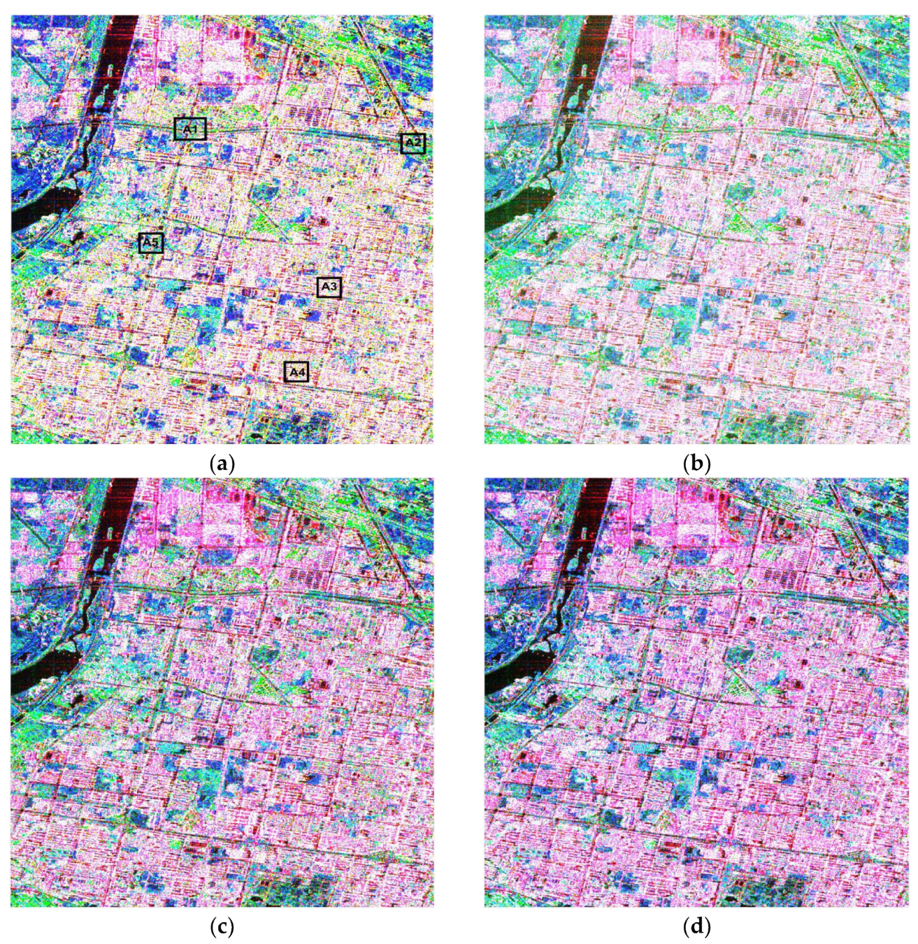
Firstly, the algorithm proposed in this article is validated using the GF-3 [8] C-band PolSAR data. The color-coded images are shown in Figure 2.

The GF-3 [8] C-band PolSAR data is over Xi’an, the fully polarimetric data were acquired on 11 July 2017, the image size is $2200\times 1900$ pixels, and the spatial resolution is about $8.03 \mathrm{m}\times 4.17 \mathrm{m}$. Figure 2a–c show the color-coded images of the Y4R, S4R, and G4U methods, while the color-coded image of the proposed four-component decomposition method is shown in Figure 2d. In this demonstration, the volume scattering power $P_{\mathrm{V}}$ is colored green, while the double-bounce scattering power $P_{\mathrm{D}}$ and odd-bounce scattering power $P_{\mathrm{S}}$ are colored red and blue, respectively. During data processing, according to (45), the data accuracy is set to $\gamma {=10}^{-6}$, and 99% of the data meets the requirement. The data used above is mainly from urban areas, so there are many buildings, which also means that double-bounce scattering should be dominant. At the same time, it can be intuitively seen from Figure 2 that the red color of the urban areas is enhanced in Figure 2d as compared with Figure 2a–c. This is because the method proposed in this article concentrates the energy of off-diagonal terms in the coherency matrix that are not used for decomposition on the terms participating in the decomposition, so that the energy of the coherency matrix is fully utilized. At the same time, this enhanced red color in the building area is beneficial for easier identification of artificial structures in vegetation areas.

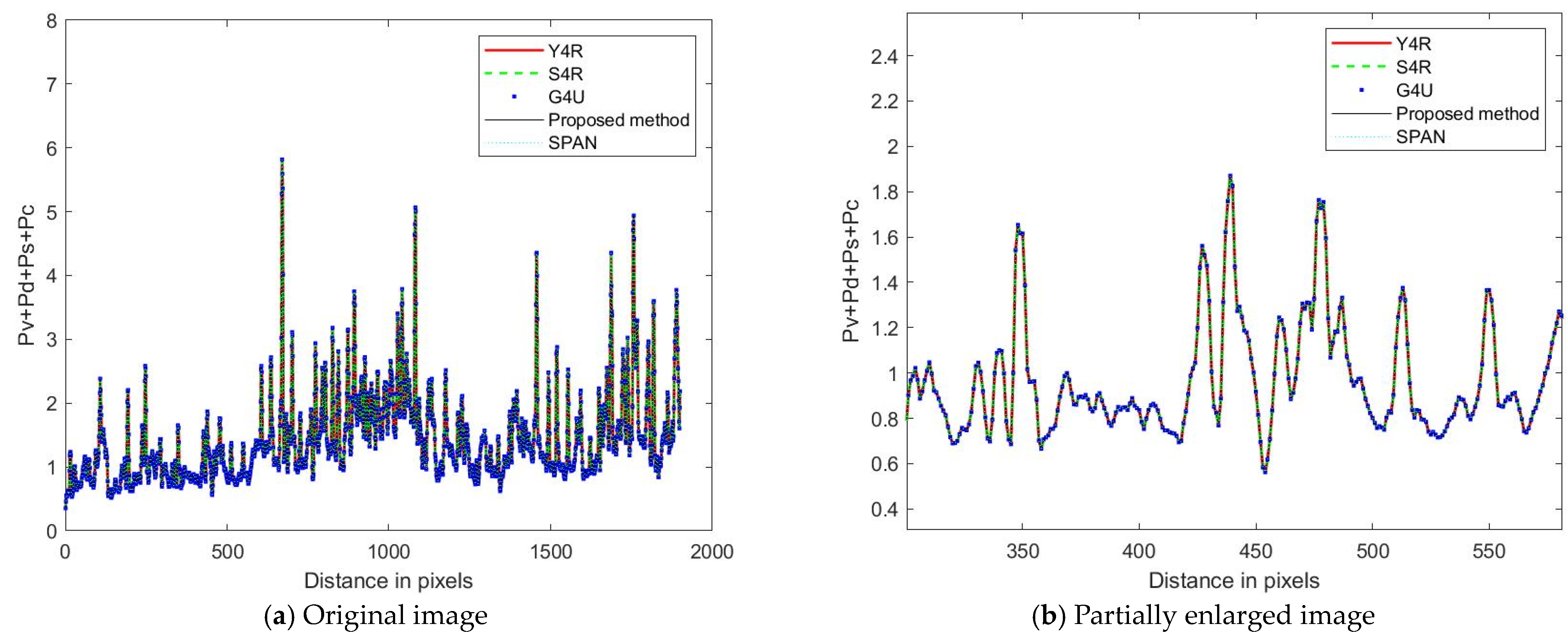
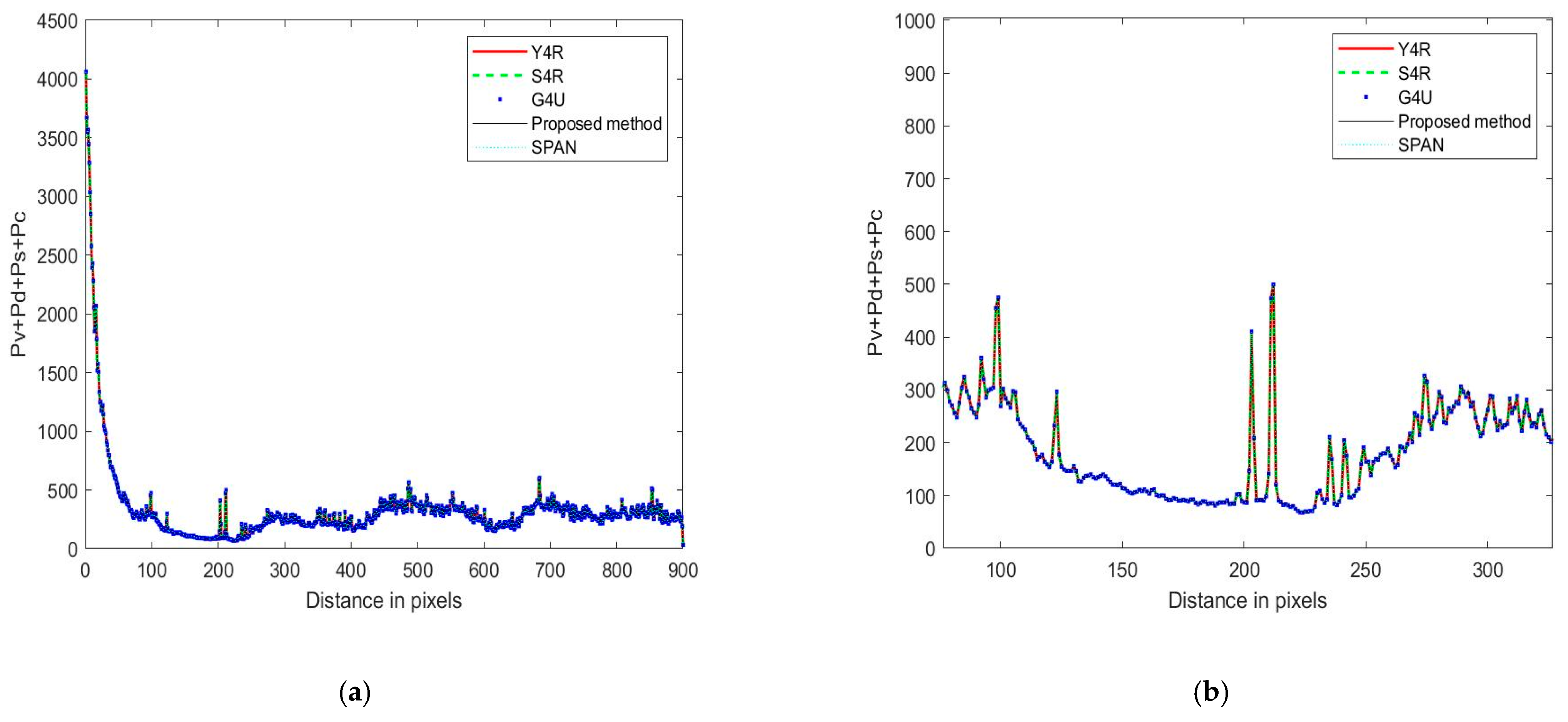
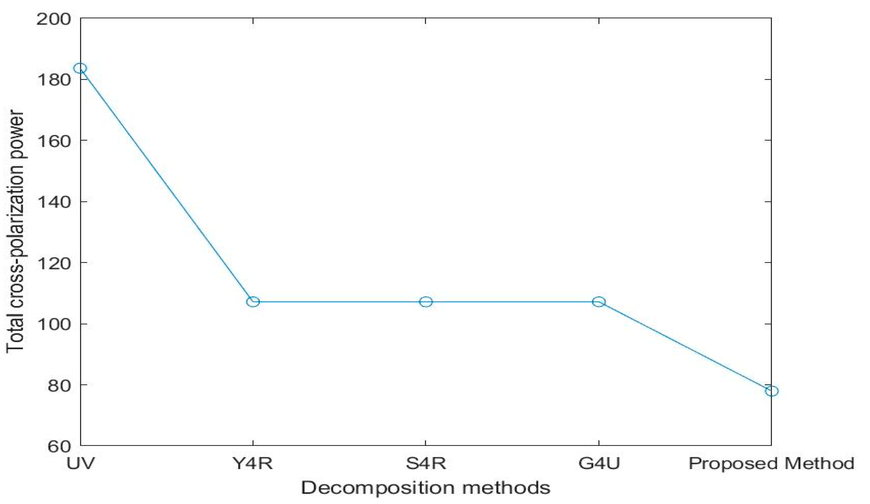
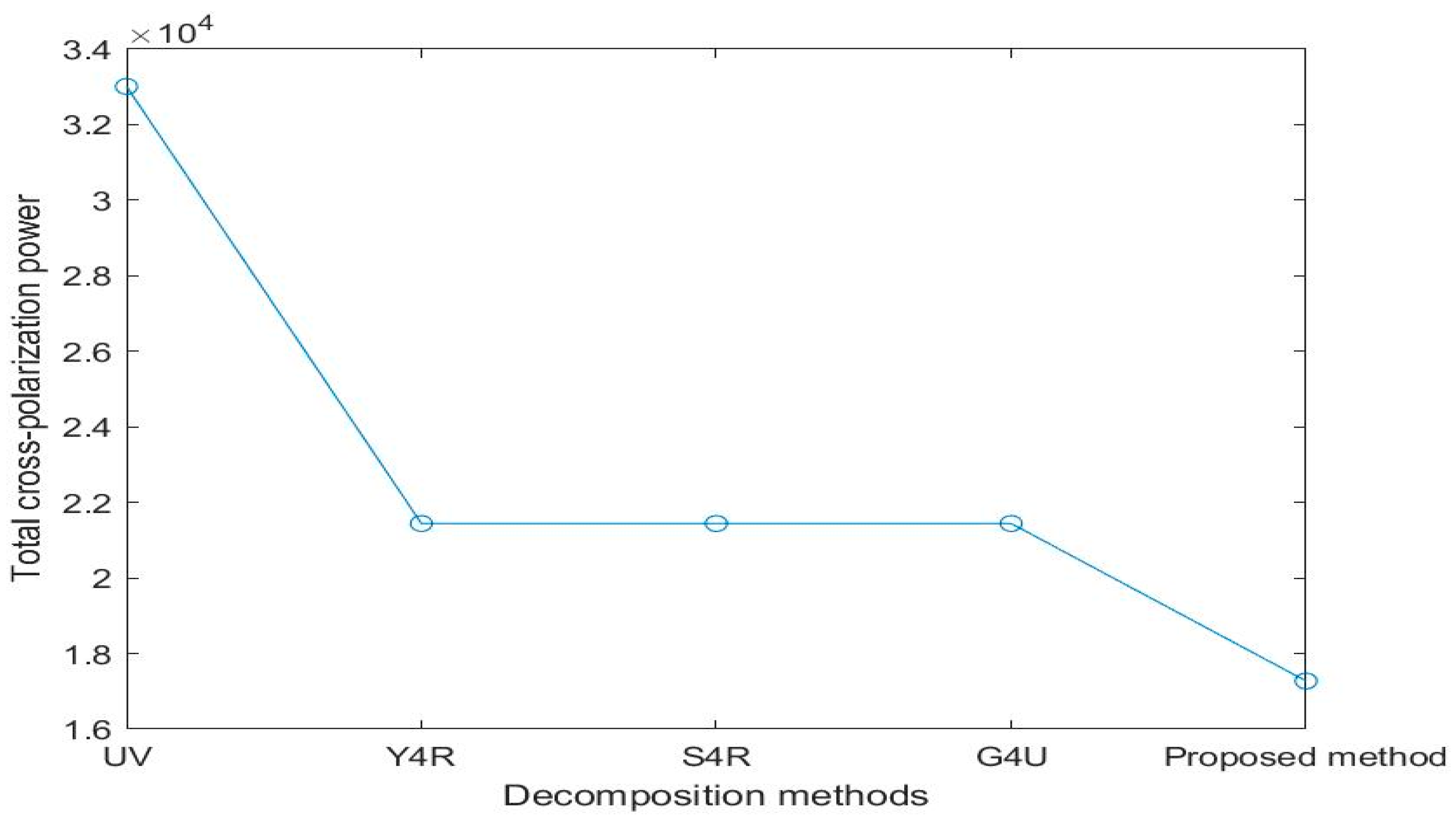
In order to verify the ability to maintain total energy, the summation $P_{\mathrm{V}}+P_{\mathrm{D}}+P_{\mathrm{S}}+P_{\mathrm{C}}$ of each pixel along the distance direction is compared with the total SPAN of each pixel along the same distance direction, as shown in Figure 3. At the same time, as several methods have compressed the energy of the cross-polarization $T_{33}$, the results of several methods can be seen in Figure 4, where UV represents the total energy of the unprocessed coherency matrix cross-polarization $T_{33}$.

Figure 3a is the original image of the $P_{\mathrm{V}}+P_{\mathrm{D}}+P_{\mathrm{S}}+P_{\mathrm{C}}$ results along the distance direction by Y4R, S4R, G4U, and the proposed method. In order to present the results more clearly, Figure 3b selected a portion of Figure 3a for magnification. From both Figure 3a,b, it can be seen that the $P_{\mathrm{V}}+P_{\mathrm{D}}+P_{\mathrm{S}}+P_{\mathrm{C}}$ results of the proposed method and existing methods are basically consistent with the total energy SPAN along the distance direction, which is similar to the conclusion in [4] that Y4R, S4R, and G4U are consistent with the total energy SPAN.

Due to the fact that Y4R, S4R, G4U, and the proposed methods all reduce the overestimation of volume scattering by reducing cross-polarization energy, Figure 4 shows the total energy of the cross-polarization term $T_{33}$ as an unprocessed coherency matrix processed by different methods. From Figure 4, it can be seen that, compared with the other three methods, the proposed method has the most significant reduction in total energy of cross-polarization. Compared to methods such as Y4R, S4R, and G4U, the total energy of cross-polarization proposed in this paper has been reduced by approximately 27%.

When $P_{\mathrm{V}}+P_{\mathrm{D}}+P_{\mathrm{S}}+P_{\mathrm{C}}$ is consistent with SPAN, the reduction of cross-polarization power will cause changes in the power of volume scattering, as can be seen from the analysis in Section 4. Therefore, to further verify the scattering results of the newly developed four-component decomposition method, the composition power profile results of different methods along the distance direction for the entire image are shown in Figure 5, Figure 6 and Figure 7. 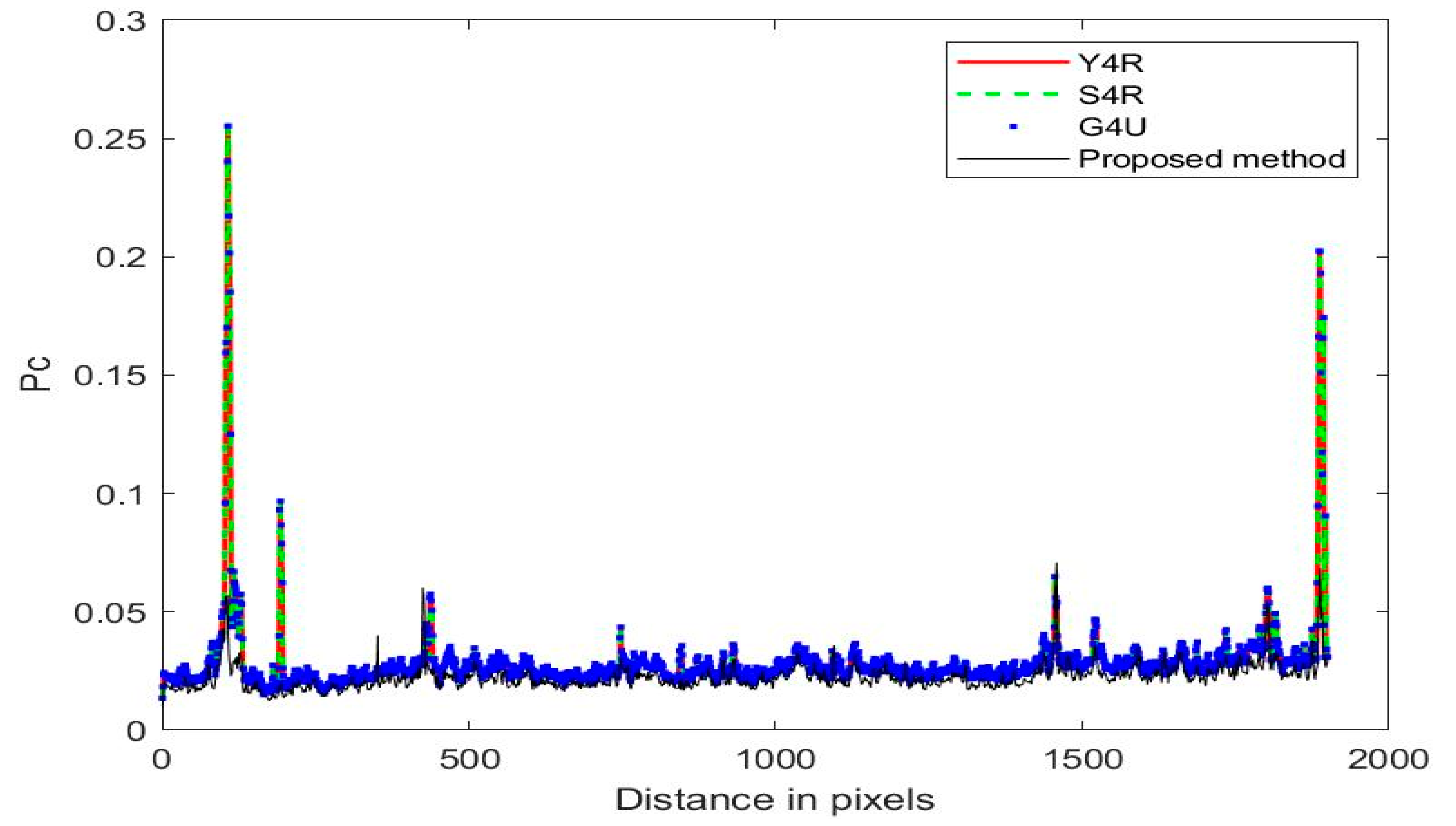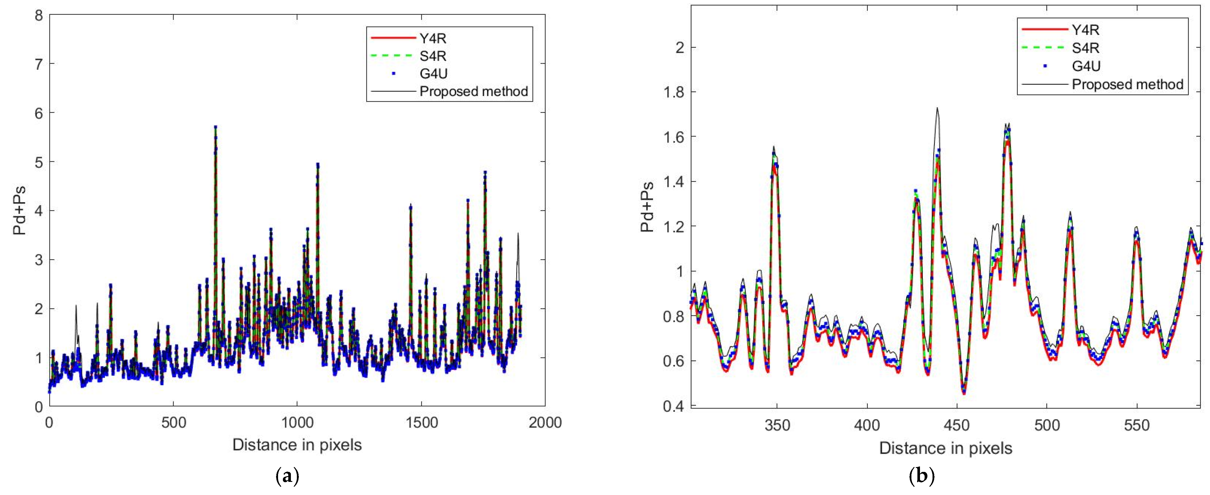Figure 5 and Figure 6 represent the power profiles for helix scattering and volume scattering along the distance direction, respectively, and Figure 7 shows the sum of the power distribution along the distance direction for double-bounce scattering and odd-bounce scattering. Similarly, in order to make the details clearer, Figure 7 is divided into the original image in Figure 7a and a partially enlarged image in Figure 7b for display.

Figure 5 shows the power of helix scattering by different methods along the distance direction. From Figure 5, it can be seen that, for the entire image, compared with existing methods, the newly developed four-component decomposition method has lower helix scattering power than the Y4R, S4R, and G4U methods. At the same time, Figure 6 demonstrates the volume scattering power of different methods along the distance direction. The results are consistent with the helix scattering power results, indicating that the proposed method has a lower volume scattering power. In other words, the helix scattering and volume scattering powers of the proposed method have been suppressed.

Figure 7 shows the sum of double-bounce scattering and odd-bounce scattering along the distance direction using different methods. Figure 7a is the original image of the $P_{\mathrm{D}}+P_{\mathrm{S}}$ results along the distance direction by Y4R, S4R, G4U, and the proposed method. Figure 7b is an enlarged view of a segment in Figure 7a, which is for the purpose of presenting the results more clearly. From the figures, it can be seen that for the entire graph, the sum of double-bounce scattering power and odd-bounce scattering power along the distance direction is higher than the other methods; in other words, the sum of double-bounce scattering and odd-bounce scattering has been improved.

Furthermore, in order to quantitatively compare the decomposition results of different methods, the relevant methods include Y4R, S4R, and G4U mentioned earlier, as well as recent literature in the model-based category, such as Maurya1 [20], Maurya2 [23], and An [24]. Maurya1, Maurya2, and An are three-component decomposition methods, where Maurya2 and An use hybrid decomposition techniques; that is, they determine the volume scattering power through eigenvalue decomposition, followed by model-based decomposition using unitary transformation. Different patches are selected, as shown in Figure 2a. Here, building areas are given special attention: patches A1 and A2 are flyovers, and patches A3 and A4 are buildings. At the same time, consideration was also given to the garden area in the city, as shown in patch A5. The quantitative comparison results for different regions based on the normalized average values of decomposed scattering power are provided in

Table 1. Normalized average four-component scattering power of patches A1–A4 in Figure 2a.

GF-3	Methods	${\mathit{P}}_{\mathbf{V}}$	${\mathit{P}}_{\mathbf{D}}$	${\mathit{P}}_{\mathbf{S}}$	${\mathit{P}}_{\mathbf{C}}$
Patch A1	Y4R	28.98	38.12	26.22	6.68
	S4R	24.64	39.23	29.45	6.68
	G4U	25.75	38.53	29.04	6.68
	Maurya1	33.08	37.66	29.26	-
	Maurya2	22.22	44.84	32.94	-
	An	22.22	49.93	27.85	-
	Proposed method	19.68	44.23	31.12	4.97
Patch A2	Y4R	34.34	34.70	24.15	6.81
	S4R	29.85	36.15	27.19	6.81
	G4U	30.71	35.69	26.79	6.81
	Maurya1	33.32	36.02	30.66	-
	Maurya2	18.94	41.47	39.59	-
	An	18.94	54.72	26.34	-
	Proposed method	24.75	40.86	28.79	5.60
Patch A3	Y4R	6.76	80.22	11.88	1.14
	S4R	4.34	80.80	13.72	1.14
	G4U	4.51	80.89	13.46	1.14
	Maurya1	7.43	80.04	12.53	-
	Maurya2	4.95	82.21	12.84	-
	An	4.95	82.81	12.24	-
	Proposed method	3.17	82.75	13.29	0.79
Patch A4	Y4R	11.08	71.90	14.81	2.21
	S4R	7.10	72.99	17.70	2.21
	G4U	7.25	73.11	17.43	2.21
	Maurya1	13.66	71.12	15.22	-
	Maurya2	9.24	74.54	16.22	-
	An	9.24	76.26	14.50	-
	Proposed method	5.63	76.27	16.57	1.53
Patch A5	Y4R	39.84	29.77	25.93	4.46
	S4R	37.09	30.40	28.05	4.46
	G4U	37.56	29.79	28.19	4.46
	Maurya1	32.71	30.78	36.51	-
	Maurya2	14.72	47.07	38.21	-
	An	14.72	54.49	30.79	-
	Proposed method	32.16	34.12	30.18	3.54

, and the total power of different regions is shown in (3).

Table 1 analyzes the normalized average values of the four scattering mechanisms, different types of terrain are selected as shown in Figure 2a. Due to the fact that Maurya1, Maurya2, and An are three-component decompositions, their decomposition results do not include helix scattering $P_{\mathrm{C}}$. Patch A1 and patch A2 are flyovers, as can be seen from Figure 2a. For flyovers, their architecture is similar to urban constructions, and scattering should be mainly double-bounce scattering and odd-bounce scattering. For patch A1, the percentages of volume scattering $P_{\mathrm{V}}$ contribution are 28.98%, 24.64%, 25.75%, and 19.68% for Y4R, S4R, G4U, and the proposed method, while the results of Maurya1, Maurya2, and An are 33.08%, 22.22%, and 22.22%, respectively. At the same time, for patch A2, the results of the volume scattering $P_{\mathrm{V}}$ contribution of several methods are as follows: 34.34%, 29.85%, 30.71%, 33.32%, 18.94%, 18.94% and 24.75%, respectively. In other words, for model-based decomposition methods Y4R, S4R, G4U, and Maurya1, the method proposed in this paper can reduce the volume scattering of Patch A1 and patch A2 by up to 13.4% and 8.59%, respectively. For the hybrid three-decomposition methods Maurya2 and An, the volume scattering power $P_{\mathrm{V}}$ is solved by $\det \left(\left[T\right]-P_{\mathrm{V}}\left[T_{\mathrm{V}}\right]\right)=0$, so $P_{\mathrm{V}}$ of these two methods are the same. From the equation, three eigenvalues can be obtained, ${\lambda }_1,{\lambda }_2,{\lambda }_3$, then $P_{\mathrm{V}}=\min \left\{{\lambda }_1,{\lambda }_2,{\lambda }_3\right\}$, which leads to better suppression of volume scattering compared to fully model-based decomposition and improves the proportion of double-bounce scattering and odd-bounce scattering. For the model-based decomposition method, the odd-bounce scattering $P_{\mathrm{D}}$ of the two flyovers has been improved by 6.57% and 6.16% by the proposed method, respectively, while the hybrid three-decomposition methods can further increase the odd-bounce scattering contribution of the two flyovers by up to 5.7% and 13.86% on the basis of the method proposed in this article. When the total power is consistent, as shown in Figure 3, the increase in the proportion of double-bounce scattering $P_{\mathrm{D}}$ and odd-bounce scattering $P_{\mathrm{S}}$ is due to the decrease in the proportion of volume scattering $P_{\mathrm{V}}$. For the four-component decomposition methods Y4R, S4R, G4U, and the proposed method, the proportion of helix scattering $P_{\mathrm{C}}$ decreased by 1.71% and 1.21%, respectively.

Patch A3 and patch A4 are built-up areas. Based on Figure 2a, they are dominated by double-bounce scattering. For patch A3, the percentages of double-bounce scattering contribution are 80.22%, 80.80%, 80.89%, 80.04%, and 82.75% for Y4R, S4R, G4U, Maurya1, and proposed method, respectively. At the same time, for patch A4, the results of several methods are as follows: 71.90%, 72.99%, 73.11%, 71.12%, and 76.27%. For odd-bounce scattering, the results of the two built-up areas have increased by 1.41% and 1.76%, respectively. At the same time, the proportion of volume scattering is reduced by 4.26% and 8.03%, respectively, while the proportion of helix scattering decreases by 0.35% and 0.68%, respectively. At the same time, for the hybrid three-component decomposition methods Maurya2 and An, the proportions of volume scattering are 4.95% and 9.24%, which are higher than the proportion of volume scattering in the proposed method. In other words, in patch A3 and patch A4, the proposed method can achieve higher proportions of double-bounce scattering and odd-bounce scattering than Maurya2 and An.

Patch A5 is a garden area in the city; both the color in Figure 2a and the data results in Table 1 indicate that the volume scattering in this area is enhanced relative to the built-up areas. The proposed four-component decomposition method also enhances the proportion of double-bounce scattering and odd-bounce scattering in the region, the percentages of volume scattering contribution are 39.84%, 37.09%, 37.56%, 32.71%, and 32.16%, for Y4R, S4R, G4U, Maurya1, and the proposed method, respectively. The proportions of double-bounce scattering and odd-bounce scattering increased by 4.35% and 4.25%, respectively. However, in this garden area, the percentages of the volume scattering contribution of Maurya2 and An are 14.72%, which is much lower than other methods. Furthermore, by observing the results of Maurya2, it can be seen that the sum of normalized powers is not equal to 100%, which means that this method did not fully decompose the energy.

5.2. AIRSAR L-Band PolSAR Dataset

In order to further verify the introduced four-component decomposition scheme, another color-coded image is provided in Figure 8. The PolSAR dataset was acquired by using AIRSAR L-band. The color-coded images are shown in Figure 8.

The fully polarimetric data were acquired on 11 May 1999 over San Francisco. The image size is $900\times 1024$ pixels, and the spatial resolution is about $10 \mathrm{m}\times 10 \mathrm{m}$.

Similar to the validation of the GF-3 dataset, the color-coded images of Y4R, S4R, G4U, and the proposed method are shown in Figure 8a–d, where the volume scattering power $P_{\mathrm{V}}$ is colored green, while the double-bounce scattering power $P_{\mathrm{D}}$ and odd-bounce scattering power $P_{\mathrm{S}}$ are colored red and blue, respectively. At the same time, the $P_{\mathrm{V}}+P_{\mathrm{D}}+P_{\mathrm{S}}+P_{\mathrm{C}}$, total power of cross-polarization, $P_{\mathrm{C}}$, $P_{\mathrm{V}}$, and $P_{\mathrm{D}}+P_{\mathrm{S}}$ results of different methods are shown in Figure 9, Figure 10, Figure 11, Figure 12 and Figure 13.

From Figure 8, it can be seen that the mountainous areas covered with forests and built-up areas are mainly dominated by volume scattering and double-bounce scattering mechanisms, respectively, while the water area is dominated by odd-bounce scattering. At the same time, it can be intuitively seen that the red color of the urban areas is enhanced in Figure 8d as compared with Figure 8a–c. This is because the method in this article concentrates the energy of off-diagonal terms in the coherency matrix that are not used for decomposition on the terms participating in the decomposition, so that the energy of the coherency matrix is fully utilized.

The analysis method is consistent with the GF-3 dataset. Figure 9a is the original image of the $P_{\mathrm{V}}+P_{\mathrm{D}}+P_{\mathrm{S}}+P_{\mathrm{C}}$ results along the distance direction by Y4R, S4R, G4U, and the proposed method. In order to present the results more clearly, Figure 9b selected a portion of Figure 9a for magnification. From Figure 3a,b, the $P_{\mathrm{V}}+P_{\mathrm{D}}+P_{\mathrm{S}}+P_{\mathrm{C}}$ results of the newly developed four-component decomposition method are basically consistent with the existing methods and total energy SPAN along the distance direction.

For the power of cross-polarization terms $T_{33}$, Figure 10 shows the results processed by Y4R, S4R, G4U, and the newly developed four-component decomposition method. Compared with the unprocessed coherency matrix, the total power of cross-polarization after being processed by different methods, such as Y4R, S4R, G4U, and the proposed method, has been reduced. At the same time, compared to Y4R, S4R and G4U, the proposed method has the most significant reduction in total energy of cross-polarization, which can be reduced by approximately 20%.

Figure 11 shows the power of helix scattering by different methods along the distance direction, and Figure 12 demonstrates the volume scattering power of different methods along the distance direction. From the results in Figure 11 and Figure 12, it is evident that the newly developed method has a lower helix scattering power and volume scattering power than the Y4R, S4R, and G4U methods, which means that the newly developed four-component decomposition method further overcomes the overestimation of volume scattering and helix scattering. This result is similar to the results of the GF-3 dataset.

Like the GF-3 dataset, the sum of double-bounce scattering and odd-bounce scattering $P_{\mathrm{D}}+P_{\mathrm{S}}$ was also analyzed, as shown in Figure 13. Where Figure 13a is the original image of the $P_{\mathrm{D}}+P_{\mathrm{S}}$ results along the distance direction by Y4R, S4R, G4U, and the proposed method. Figure 13b is an enlarged image. From the figures, the result of the newly developed four-component decomposition method is higher than the other methods, which reduces the impact of volume scattering.

Similar to the analysis in the previous section, different patches are selected as shown in Figure 8a. The Y4R, S4R, G4U, Maurya1 [20], Maurya2 [23], and An [24] decomposition methods are compared with the method proposed in this paper. At the same time, the percentage of the normalized mean of scattering powers by different methods for these selected patches is calculated in

Table 2. Normalized average four-component scattering power of patches A1-A4 in Figure 8a.

AIRSAR	Methods	${\mathit{P}}_{\mathbf{V}}$	${\mathit{P}}_{\mathbf{D}}$	${\mathit{P}}_{\mathbf{S}}$	${\mathit{P}}_{\mathbf{C}}$
Patch A1	Y4R	16.80	63.71	16.69	2.80
	S4R	11.04	66.02	20.14	2.80
	G4U	11.12	66.57	19.51	2.80
	Maurya1	15.77	63.22	21.01	-
	Maurya2	5.62	69.38	25.00	-
	An	5.62	74.13	20.25	-
	Proposed method	7.90	69.63	20.76	1.71
Patch A2	Y4R	26.91	50.53	17.37	5.19
	S4R	20.05	53.43	21.33	5.19
	G4U	20.41	53.77	20.63	5.19
	Maurya1	25.20	48.33	26.47	-
	Maurya2	8.51	59.45	32.04	-
	An	8.51	68.26	23.23	-
	Proposed method	14.17	58.33	23.95	3.55
Patch A3	Y4R	15.12	66.43	16.03	2.42
	S4R	10.02	68.23	19.33	2.42
	G4U	10.02	68.54	19.02	2.42
	Maurya1	14.41	66.01	19.58	-
	Maurya2	5.67	71.42	22.91	-
	An	5.67	75.12	19.21	-
	Proposed method	6.96	71.64	20.05	1.35
Patch A4	Y4R	57.91	15.15	12.31	14.63
	S4R	53.68	17.29	14.44	14.59
	G4U	54.55	16.89	13.93	14.63
	Maurya1	38.31	24.85	36.84	-
	Maurya2	11.69	39.16	49.15	-
	An	11.69	61.55	26.76	-
	Proposed method	40.50	26.77	21.87	10.86
Patch A5	Y4R	6.03	0.36	92.72	0.89
	S4R	6.03	0.36	92.72	0.89
	G4U	6.03	0.39	92.69	0.89
	Maurya1	5.35	0.89	93.76	-
	Maurya2	2.16	1.42	96.42	-
	An	2.16	1.32	96.52	-
	Proposed method	2.47	2.65	94.75	0.13

. Here, urban areas are given special attention (patches A1 to A4); among these urban patches, patch A4 is an urban area with vegetation, while water areas were also studied (patch A5), as shown in Figure 8a.

The observations made for the GF-3 image also apply to the AIRSAR image. In the AIRSAR image, patches A1 to A3 are all urban areas, and the difference between patch A1, patch A2, and patch A3 lies in their different orientation angles. Patch A1 and patch A3 have similar orientation angles but different orientation angles from patch A2, as can be seen from Figure 8a. For Y4R, S4R, G4U, Maurya1, and the proposed method, patch A1 and patch A3 with similar orientation angles, an additional increment of 5.92% and 5.21% by the newly four-component decomposition method of double-bounce scattering $P_{\mathrm{D}}$ compared with the Y4R method, 3.61% and 3.41% compared with the S4R method, 3.06% and 3.10% compared with the G4U method, and 6.41% and 5.63% compared with the Maurya1 method, respectively. For urban patch A2, there is a similar result as for patch A1 and patch A3. The proportion of double-bounce scattering $P_{\mathrm{D}}$ by the newly developed method has increased compared to the Y4R, S4R, G4U, and Maurya1 decomposition methods; the result can be 10%. The increase in the proportion of double-bounce scattering means a more accurate interpretation of urban areas. In the vegetation patch A4 case, the contribution of the volume scattering component is 40.50% by the newly developed four-component decomposition method. As can be seen from Figure 8a, the selected vegetation area lies in the urban region; hence, this vegetation patch also expects significant odd-bounce scattering and double-bounce scattering mechanisms. The water area in patch A5 exhibits blue, so the odd-bounce scattering contribution is dominant. The percentages of odd-bounce scattering contribution are 92.72%, 92.72%, 92.69%, 93.76, and 94.75% for Y4R, S4R, G4U, Maurya1, and the proposed method, respectively, which is consistent with reality. For the hybrid three-component decomposition methods Maurya2 and An, the experimental results are similar to those of GF-3.

In the hybrid decomposition methods Maurya2 and An, since the volume scattering power is first determined based on the minimum $P_{\mathrm{V}}$ that satisfies $\det \left(\left[T\right]-P_{\mathrm{V}}\left[T_{\mathrm{V}}\right]\right)=0$, and then model-based decomposition is performed through different unitary transformations, Maurya2 and An have the same volume scattering power. From the results of the GF-3 and AIRSAR datasets, it can be seen that the hybrid decomposition methods exhibit significant advantages in built-up areas, especially in highly oriented urban structures (patch A4 of the AIRSAR dataset), which can increase the proportion of double-bounce scattering and odd-bounce scattering. However, in vegetation areas, as $P_{\mathrm{V}}$ is the minimum value that satisfies $\det \left(\left[T\right]-P_{\mathrm{V}}\left[T_{\mathrm{V}}\right]\right)=0$, this hybrid method will underestimate the volume scattering power, as can be seen in patch A5 of the GF-3 dataset. Compared with other methods, the proportion of volume scattering in the hybrid method can be reduced by up to 25.12% in these vegetation areas. The method proposed in this paper is based on four basic scattering models, which can avoid underestimation of volume scattering by hybrid methods in vegetation areas to some extent. At the same time, compared to other model-based methods, the method proposed in this paper can achieve better performance.

5.3. Iteration Number and Accuracy Analysis

For an iterative approach, the iteration number $n$ is very important, given the fact that $n$ cannot be infinite in practice. For this paper, we take the GF-3 C-band PolSAR dataset ($2200\times 1900$ pixels) as an example to analyze the impact of iteration number $n$ from different aspects.

The number of iterations is closely related to the accuracy requirements. Therefore, this paper first analyzes the number of iterations required for data to meet different accuracies. Here, the iteration numbers required for 96%, 97%, 98%, 99%, and 100% of the GF-3 dataset to meet different accuracies are analyzed. The termination conditions $\gamma$ shown in (45) have accuracies of ${10}^{-4}$, ${10}^{-5}$, ${10}^{-6}$ and ${10}^{-7}$,respectively. The iteration number $n$ under different accuracies and data proportions is calculated in

Table 3. Iteration number $n$ under different accuracies and data proportions.

Proportion	96%	97%	98%	99%	100%
Accuracy
${10}^{-4}$	_	_	1	2	5
${10}^{-5}$	4	5	7	11	27
${10}^{-6}$	12	15	19	30	68
${10}^{-7}$	23	27	35	50	119

.

From the above results, it can be seen that when the accuracy requirement is low, a simple iteration can meet the requirements. However, when the accuracy requirement is higher, the number of iterations increases, but it can be achieved through a limited number of operations. Due to the different pixels, the number of iterations that satisfy both $T_{13}$ and $\mathrm{Re}\left(T_{23}\right)$ close to zero is also different. Therefore, in reality, this paper fixes the maximum iteration number $N$ in (45). Here, we take $N=20$ and analyze the proportion of data that satisfies different data accuracies under the maximum iteration number; the results are shown in

Table 4. The proportion of data satisfying different accuracies when $N=20$.

Accuracy	${10}^{-4}$	${10}^{-5}$	${10}^{-6}$	${10}^{-7}$
Proportion	100%	99.67%	98.17%	95.19%

.

Furthermore, this paper achieves minimization of the cross-polarization term $T_{33}$ by decoupling the off-diagonal terms that do not participate in the four-component decomposition. Therefore, this paper also analyzes the impact of data accuracy. The total power of cross-polarization under different accuracies is shown in

Table 5. Total power of cross-polarization at different accuracies.

Accuracy	${10}^{-4}$	${10}^{-5}$	${10}^{-6}$	${10}^{-7}$
Total power of cross-polarization	110.88	82.06	78.02	77.88

below. Assuming 99% of the data meets the accuracy requirement, the number of iterations under different accuracies is shown in Table 3.

The results in Table 5 indicate that through the processing of the method proposed in this manuscript, as the data accuracy improves, the total power of cross-polarization moves to a stable result, which is consistent with the results of previous theoretical analyses.

Finally, computational time is considered in this manuscript. Here, the time cost of different methods was calculated by taking the patch A3 area in the GF-3 data as an example. The computational time of the method proposed was conducted with $N=20$ and $\gamma ={10}^{-6}$. In the experiment, a local PC with an Intel Core i7 CPU and 16 GB of memory was used to process the data set. The results are shown in

Table 6. Computational time of different methods.

Mehods	Y4R	S4R	G4U	Maurya1	Maurya2	An	Proposed Method
Computational time(s)	6.78	5.96	6.28	5.53	819.25	824.57	8.24

below.

From Table 6, it can be seen that the model-based decomposition methods, including Y4R, S4R, G4U, and Maurya1, consume less computational time than other investigated methods. The proposed method in this paper involves iterative operations and takes relatively more computational time than those compared with the model-based methods shown in Table 6. However, the computational time of the model-based methods is at the same level. The hybrid decomposition methods, including Maurya2 and An, have the longest computational times among all the methods. The reason is that the hybrid decomposition method involves solving matrix eigenvalues, which means the procedure of eigendecomposing the covariance matrix with the computational complexity of $O(N^3)$ ($N$ is the dimension of the covariance matrix).

6. Conclusions

In this paper, a methodology is proposed to optimize the fully coherency matrix of PolSAR. This method utilizes the properties of the Jacobi method through unitary transformation to concentrate the energy of off-diagonal terms that do not participate in model-based four-component decomposition on other terms, which means reducing the nine parameters of the coherency matrix to the six required for decomposition. Additionally, the proposed method avoids the generation of residual matrices without the assumption of scattering symmetry and can minimize the volume scattering power in four-component decomposition. The effectiveness of the newly developed four-component decomposition method was investigated by using the GF-3 C-band and AIRSAR L-band PolSAR datasets. The experiment shows that the newly developed method can effectively reduce the energy of the cross-polarization term, which also means that compared with the Y4R, S4R, G4U, and Maurya1 methods, the newly developed method can effectively increase the contributions of double-bounce and odd-bounce scattering in urban areas. From the analysis of the iteration number, accuracy, and computational time, it was found that the proposed method can achieve data accuracy after a finite number of iterations, and the computational time is equivalent to traditional four-component decomposition methods such as Y4R and G4U and is significantly lower than in the hybrid methods. These experiments have all verified the distinctness and superiority of this method. Therefore, Jacobi-based polarization decomposition can effectively extract features of scenes, especially urban areas, which provides a more suitable approach for the application of PolSAR data.