Article

Anti-Rain Clutter Interference Method for Millimeter-Wave Radar Based on Convolutional Neural Network

School of Electronic and Optical Engineering, Nanjing University of Science and Technology, Nanjing 210094, China
*
Author to whom correspondence should be addressed.
Remote Sens. 2024, 16(20), 3907; https://doi.org/10.3390/rs16203907
Submission received: 27 August 2024 / Revised: 30 September 2024 / Accepted: 19 October 2024 / Published: 21 October 2024

Abstract

:
Millimeter-wave radars are widely used in various environments due to their excellent detection capabilities. However, the detection performance in severe weather environments is still an important research challenge. In this paper, the propagation characteristics of millimeter-wave radar in a rainfall environment are thoroughly investigated, and the modeling of the millimeter-wave radar echo signal in a rainfall environment is completed. The effect of rainfall on radar detection performance is verified through experiments, and an anti-rain clutter interference method based on a convolutional neural network is proposed. The method combines image recognition and classification techniques to effectively distinguish target signals from rain clutter in radar echo signals based on feature differences. In addition, this paper compares the recognition results of the proposed method with VGGnet and Resnet. The experimental results show that the proposed convolutional neural network method significantly improves the target detection capability of the radar system in a rainfall environment, verifying the method’s effectiveness and accuracy. This study provides a new solution for the application of millimeter-wave radar in severe weather conditions.

1. Introduction

With the continuous progress of science and technology, millimeter-wave radar has made remarkable development, especially in the fields of automobiles and unmanned aerial vehicles [1,2,3,4]. For example, millimeter-wave radar is used for wingtip distance measurement of high-speed coaxial helicopters, as mentioned in reference [3], and it is also applied in target detection and autonomous driving [1,2,4], among others. Millimeter-wave radar has demonstrated unique advantages in detection and imaging [5], and is gradually becoming an indispensable part of modern radar systems by virtue of its unique technical characteristics and wide application potential. However, it is due to the diversity of the application environment that millimeter-wave radar is affected by various kinds of interference in the process of practical application.
A rainfall environment, as a typical severe weather condition, has a significant impact on millimeter-wave radar. At present, the effect of rain clutter on millimeter-wave radar in rainfall environments is still an important research topic [6]. Due to the large differences in the distribution characteristics of raindrops around the globe, no uniform standard has been formed to model the signals under rainfall environments. This paper analyses the main effects of rainfall environments on millimeter-wave radar signals based on CST electromagnetic simulation, and these effects are specifically divided into two parts: the rain clutter signals generated by the reflection of raindrops, and the attenuation of the transmitted signals by the rainfall environment. Therefore, reducing the impact of rain clutter on the detection performance of millimeter-wave radar has become an important issue. However, effective methods to address this problem are still very scarce. In reference [7], a method based on two-dimensional filtering is proposed to counteract the interference of rain clutter. And after referring to some other radar anti-jamming methods [8,9], this paper chooses to use a convolutional neural network (CNN) for anti-rain clutter.
The development of CNNs dates back to the 1990s when they were first proposed by Yann LeCun et al. [10]. The earliest LeNet-5 model achieved remarkable success in handwritten digit recognition tasks. As computational power increased and datasets expanded, CNNs saw a major breakthrough in the mid-2000s. In 2012, AlexNet marked the arrival of the deep learning era by significantly improving the accuracy of image classification in the ImageNet competition [11]. In recent years, network architectures such as VGGnet, ResNet, EfficientNet and MobileNetV3 have continued to push the frontiers of the technology [12,13,14,15], and CNNs are now widely used in computer vision, natural language processing, and other fields [16,17,18,19]. The combination of millimeter-wave radar and CNNs opens up new applications in the field of image recognition, especially in target detection and recognition in complex environments. In reference [20], millimeter-wave radar is applied to multi-person action recognition; reference [21] uses it for target detection; while reference [22] explores its application in trajectory recognition. These studies demonstrate the potential and advantages of combining millimeter-wave radar with CNNs in a variety of tasks. This paper, on the other hand, applies CNNs to anti-interference processing of millimeter-wave radar. Initially, VGGNet was used for this task, but its recognition performance was not satisfactory. Therefore, an attempt was made to combine the VGGNet with other network structures, and the results show that this attempt was a remarkable success as the recognition performance was significantly improved.
In this paper, a CNN method is used for the anti-rain clutter process, and it is compared with VGGnet and Resnet to demonstrate the accuracy of anti-rain clutter. Such a study helps to improve the ranging measure capability of millimeter-wave radar in complex environments and provides more reliable technical support for practical applications.

2. Triangular Wave Linear Frequency Modulation Signal

The triangular wave linear frequency modulation signal is a continuous wave signal used in millimeter-wave radar. Due to its favorable spectral characteristics and controllable frequency variation patterns, this signal is commonly employed for applications such as measuring range and velocity or spectrum analysis. This study uses the triangular wave linear frequency modulation signal for ranging purposes. Figure 1 illustrates a schematic diagram of target detection using the triangular wave linear frequency modulation signal.
In Figure 1, f t t denotes the transmitted signal frequency, f r t represents the echo signal frequency, f 0 is the center frequency, Δ F m indicates the modulation bandwidth, and f i t is the beat frequency. Figure 1 shows that within one modulation period T m , the beat frequency f i t of the triangular wave frequency modulation detection system is divided into four intervals. Intervals 1 and 3 are irregular, while intervals 2 and 4 are regular. The beat frequency f i t remains stationary in the regular regions, whereas in the irregular regions, it changes linearly. In practical applications, only the signals within the regular regions are considered, and those within the irregular regions are excluded.
The frequency modulation slope of the triangular wave frequency modulation detection system is given by:
k F = Δ F m T m / 2 = 2 Δ F m T m
Within a modulation period T m , there are two segments in f i t : the rising segment f i + , and the falling segment f i . Given the delay τ = 2 R / c , the expressions for f i + and f i can be derived as follows:
f i + = f t f r = k F τ f d = 4 Δ F m R T m c f d
f i = f r f t = k F τ + f d = 4 Δ F m R T m c + f d
Adding Equations (2) and (3) gives the distance R between the target and the detector.
R = c T m 4 Δ F m f i + + f i 2
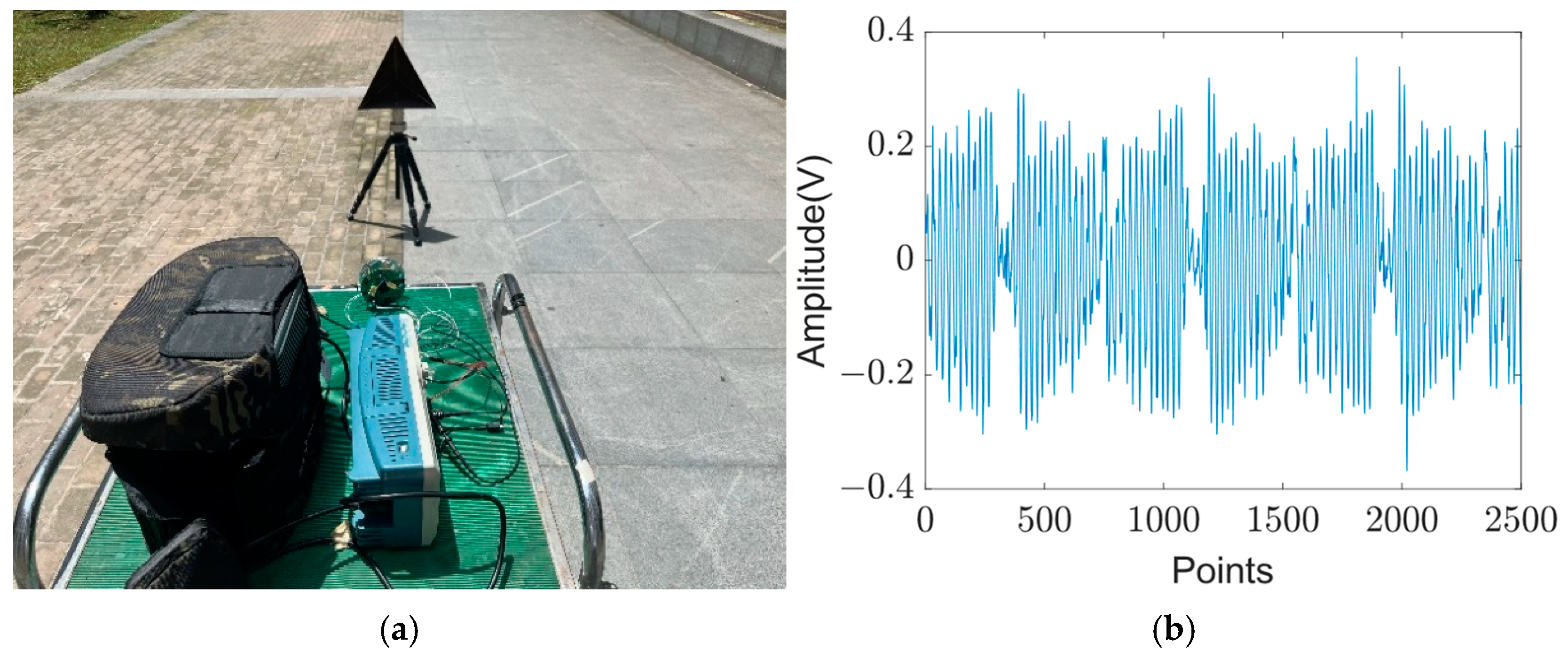
In the experimental setup shown in Figure 2a, the equipment used includes a 24 GHz triangular wave linear frequency modulation detector, a portable power supply, an oscilloscope, and a corner reflector placed 8 m from the detector. Signal sampling is performed at a rate of 100 MHz, and the sampling result is shown in Figure 2b. Using Equation (4) to measure the range; the result is 8.08 m, with the error being within an acceptable range.

3. Rain Clutter Signal

3.1. Signal Propagation in Rainfall Environments

The raindrop size distribution refers to the number of raindrops of different sizes in a unit volume at various rainfall rates, also known as the raindrop spectrum. It is a crucial parameter for studying radio wave propagation in rainfall environments. Due to varying conditions globally, the distribution of rainfall also differs. The most commonly used raindrop spectra are the negative exponential Marshall–Palmer (M-P) distribution and the Weibull distribution. In this study, the distribution model used is the M-P distribution.
Based on their measurements and incorporating data from Laws and Parsons, Marshall and Palmer proposed the M-P distribution model, which can be expressed as:
N D = N 0 e Λ D
In Equation (5):
N 0 = 8000   ( m 3 mm 1 )
Λ = 4.1 P R 0.21   ( mm 1 )
D is the raindrop diameter, P R is the rainfall rate, and N D represents the number of raindrops per cubic meter.
This paper uses CST2019 software to simulate signal propagation under rainy conditions to study its characteristics in a rainfall environment. Figure 3a shows the schematic diagram of the signal propagation modeling in a rainy environment in CST. Figure 3b depicts the raindrop modeling in CST. In the electromagnetic simulation, the number of raindrops required for space 8   m × 4   m × 4   m is calculated using the M-P model, as shown in Equation (5). These raindrops are then randomly distributed in space. A plane wave is transmitted from plane ABCD, and probes are placed at points O and P to receive the signal.
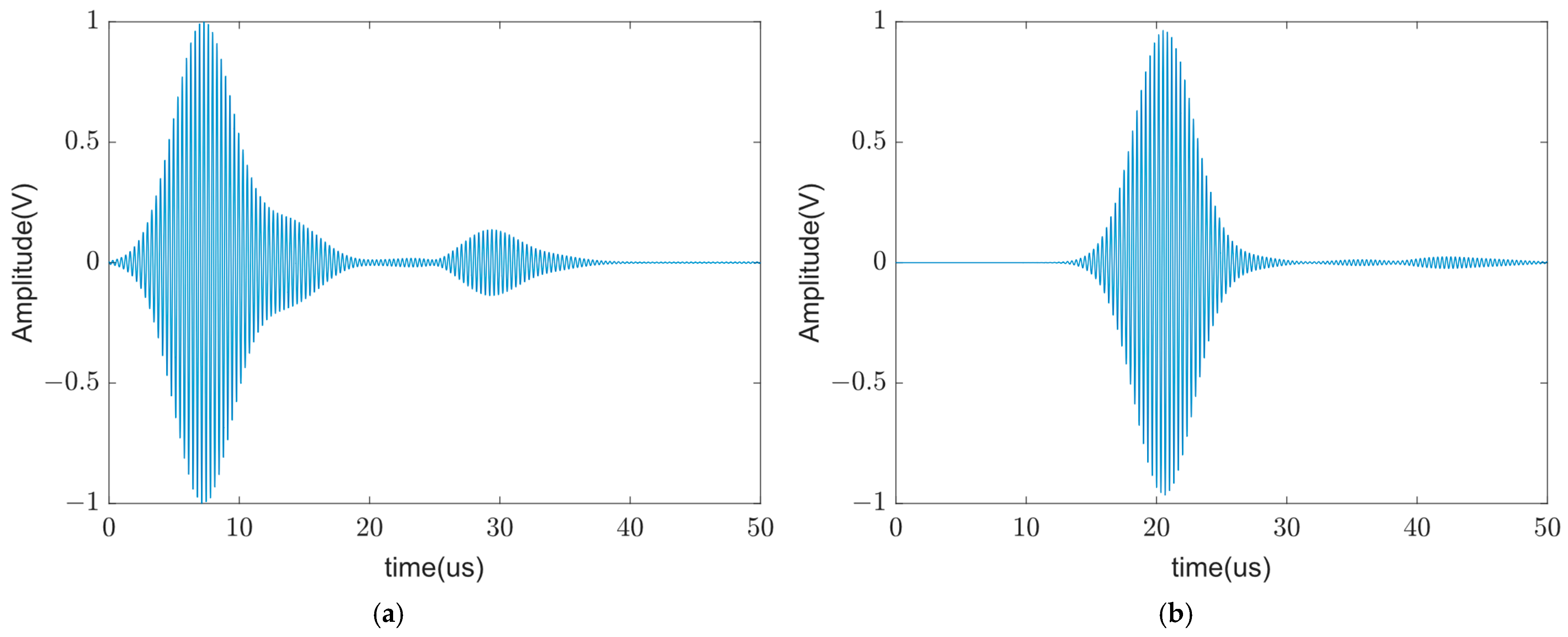
The results of the CST electromagnetic simulation are shown in Figure 4. Figure 4a presents the signal received by the probe at point O. It is evident from the figure that, in addition to the transmitted signal, the probe also receives signals reflected by raindrops. Figure 4b shows the signal received by the probe at point P. The transmitted signal is noticeably attenuated, and raindrops scatter some additional signal later. Combining the results from both figures, it can be concluded that in a rainfall environment, the impact on signal propagation consists of two main parts: first, the reflection of the signal by raindrops, and second, the attenuation of the signal due to the rainfall environment.

3.2. The Influence of the Rainfall Environment on Signals

3.2.1. Attenuation Under a Rainfall Environment

In the signal propagation process through a rainfall environment, in addition to atmospheric losses, the presence of raindrops causes additional attenuation of the signal. The radar equation for a target under the influence of a rainfall environment can be expressed as:
P r = P t G 2 λ 2 σ 4 π 3 R 4 L S e 0.46 A
In Equation (8), P t is the power of the transmitter, G is the antenna gain, λ is the operating wavelength, R is the radar range, σ is the radar cross-section, and A is the rain attenuation along the electromagnetic wave propagation path, which equals the rain attenuation rate γ R dB / Km multiplied by the path length A = γ R R , and L S represents the radar’s losses. According to the empirical formula provided by the International Telecommunication Union (ITU):
γ R = k P R α
In Equation (9), the coefficients k and α are derived by fitting the curve to a power-law coefficient through discrete calculations.
k = k H + k V + k H k V cos 2 ω cos 2 τ / 2
α = k H α H + k V α V + k H α H k V α V cos 2 ω cos 2 τ / 2 k
The parameters k H , k V , α H , and α V can be obtained from the parameter tables provided by the ITU. ω represents the path inclination angle, and τ represents the polarization inclination angle. The k H , k V , α H , and α V parameters for two typical frequencies, 24 GHz and 35 GHz , are shown in Table 1.

3.2.2. Reflected Signal Under a Rainfall Environment

In addition to direct attenuation, raindrops also cause reflection of the signal. When millimeter-wave signals encounter raindrops, some of the energy is reflected into space, creating what is known as rain clutter. These reflected signals may differ in phase from the original signal, leading to interference.
The actual conditions in a rain zone are very complex, with raindrops of various sizes distributed throughout. When a target is within the radar detection range in the rain zone, the receiver picks up rain clutter. We assume there is a small volume element d V within a small region at a beam axis tilt angle θ , an azimuth angle φ , and a distance L from the antenna. This volume element contains a small area d S perpendicular to the incident wave direction, with a radial depth d L . We then let d Ω be the solid angle of the area element. Since the volume element is small enough to ensure that all scattered energy reaches the antenna simultaneously, d V = L 2 d Ω d L can be derived. The radar-received rain scatter energy can be expressed as:
d P t = P t G 2 λ 2 4 π 3 L 4 f θ , φ 4 η R d V = P t G 2 λ 2 d L 4 π 3 L 2 f θ , φ 4 η R d Ω
Assuming the effective radial depth of the beam is h D / 2 , the effective echo distance from the radar is L L + h D / 2 . h D = c τ , where τ represents the pulse width, and c is the speed of light. The reflected echo energy from rain with a Gaussian-shaped antenna can be expressed as:
P r = P t G 2 λ 2 h D θ φ η R 1024 π 2 L 2 ln 2
In Equation (13), η R = 0 D MAX Q i , j D N D d D represents the volumetric reflectivity of raindrops, which is the backscatter cross-section. D denotes the diameter of the raindrops. Q i , j D is the backscatter cross-section of particles calculated using Mie theory. N D d D represents the drop size distribution spectrum for raindrops with a diameter of D D + d D .

3.2.3. Signal Modeling and Simulation in Rainfall Environments

First, we model the raindrop spectrum. Using Equation (5), we calculate the number of raindrops within a space 20   m × 20   m × 20   m for a given rainfall rate. Since rainfall distribution in space is random, we distribute these raindrops randomly. We generate three random arrays X 1 n , Y 1 n and Z 1 n for the X, Y, and Z coordinates, respectively, of the raindrops. Based on these coordinates, we perform raindrop spectrum modeling in the simulation.
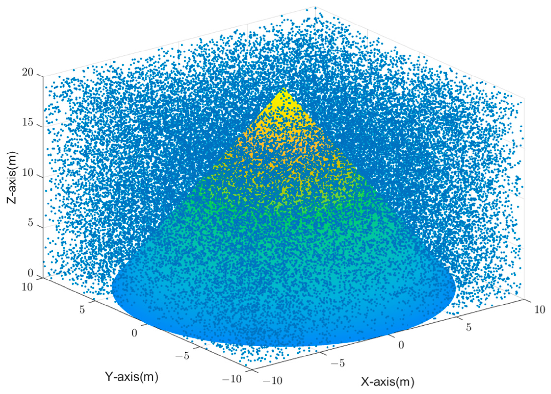
In the laboratory, the triangular wave linear frequency modulation detector has a conical detection range. To simulate the actual situation, as shown in Figure 5, the detector’s conical detection range is set to 20 m, matching the detector’s actual detection distance. In the simulation, this conical range accurately reflects the detector’s real-world operating conditions.
After setting the radar’s detection range, raindrops are assessed based on their position within the radar beam’s effective coverage. Raindrops within this range will reflect radar signals. The reflected signal energy from raindrops is calculated using Equation (13), where η R represents the sum of the backscattering cross-sections of raindrops within the same range. In this study, the backscattering cross-section of each raindrop is computed individually. Consequently, the reflected signals from all raindrops within the detection range are generated independently and then summed to obtain the overall rain clutter signal.
In the simulation environment described in this paper, the radar is located at the vertex of the cone, where the cone’s range represents the effective coverage area of the radar beam, and the target is positioned at the origin of the coordinate axis 0 , 0 , 0 . The simulated detector parameters are shown in Table 2, and the simulation results are shown in Figure 6.
From the time-domain simulation results in Figure 6a, it can be observed that the time-domain waveform of the rain clutter signal is chaotic and exhibits a complex temporal variation pattern. The frequency-domain simulation results in Figure 6b show that the signal’s frequency spectrum is predominantly concentrated in the low-frequency range, indicating that the signal’s frequency components are stronger in the low-frequency domain. Additionally, the time-frequency plot in Figure 6c provides a clear view of the signal’s energy distribution, where the energy blocks represent the ratio of signal energy to the maximum energy value, helping us understand the signal’s energy distribution characteristics in both time and frequency domains.

3.3. Signal Measurement in a Rainfall Environment

To explore the characteristics of rain clutter signals in the rainfall environment, actual signal detection experiments were conducted, which also helped verify the accuracy of the simulation results. A large umbrella was added to the experimental equipment shown in Figure 2a to prevent the equipment from becoming wet and causing short circuits. This ensured the experimental process’s reliability and the data’s accuracy.
The experimental setup is shown in Figure 7. A triangular waveform linear frequency modulation detector was used in an open environment to collect signals from a rain-affected area. The measured signals from the rainfall environment are displayed in Figure 8.
From the actual measured signal results from the experiment, it can be observed that the time-domain signal is very similar to the simulated signal, both exhibiting relatively chaotic signals with no apparent patterns. In the frequency-domain analysis, the signal energy is concentrated within 10 MHz, a fact corroborated by the spectrogram, which shows similar energy distribution to the simulated signal. However, a significant difference between the actual and simulated signals is that the simulated signal includes only signals from within a 20 m range, resulting in a zero-signal component beyond 10 MHz in the frequency spectrum. In contrast, the actual measurements, while still primarily within the 10 MHz range, also detect some weak signals beyond 10 MHz, indicating the presence of certain signal components in the higher frequency range.
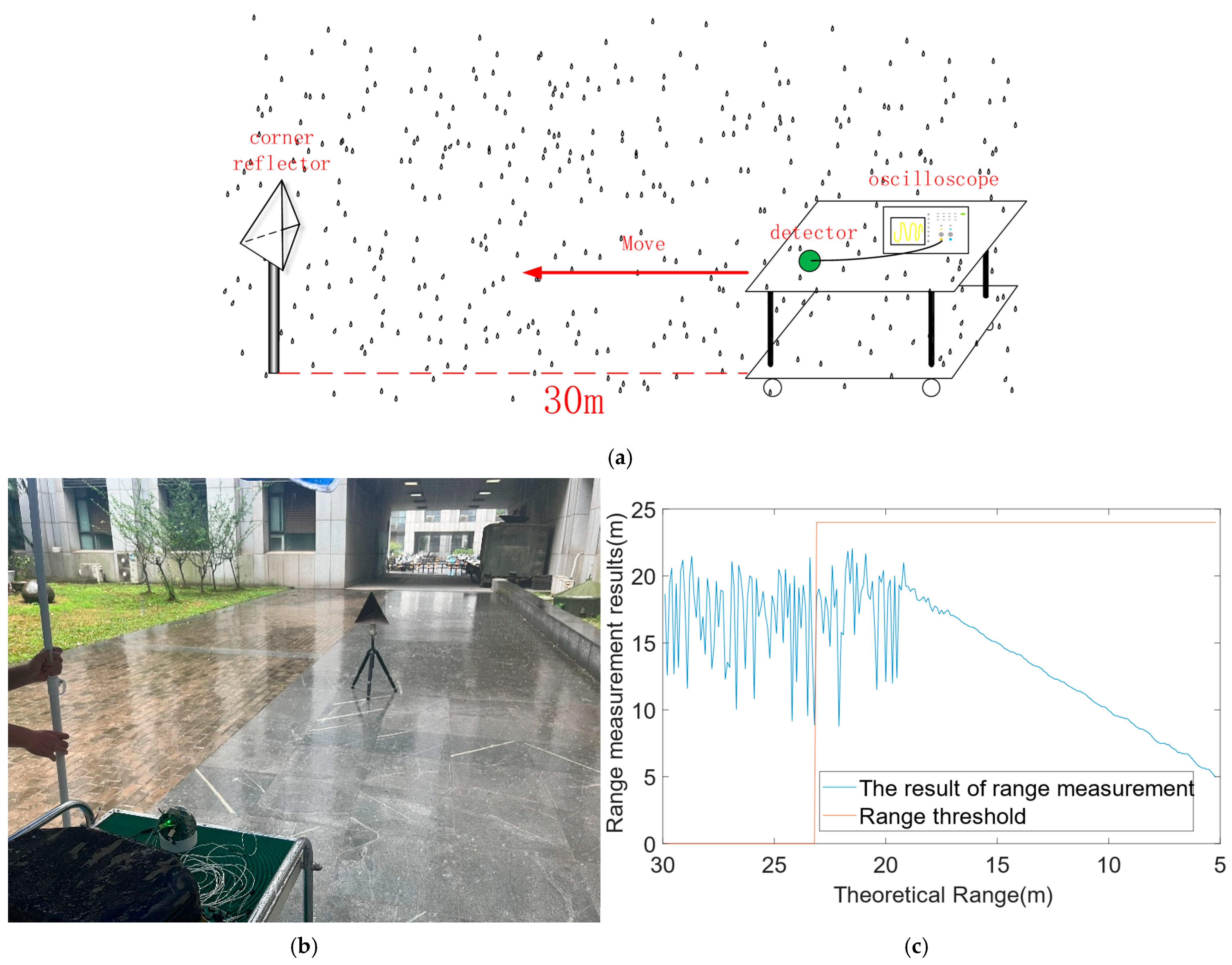
The range measurement experiment was conducted by moving the detector from a starting point 30 m from the angle reflector towards a distance of 5 m, while collecting signals in rainfall environments. The signals were then subsequently processed using a computer to measure the range using Equation (4). The schematic diagram of the experiment is illustrated in Figure 9a, and the actual experimental scene is shown in Figure 9b, while the measurement results are presented in Figure 9c. Assuming a range threshold of 9 m, the threshold is triggered when the measured distance is less than 9 m. The results indicate that measurements affected by rain clutter are uncertain and may lead to premature triggering of the range threshold. Therefore, it can be concluded that range measurements in rainfall environments are influenced to some extent, and it is necessary to propose a method to resist the influence of rain clutter on the triangular wave linear frequency modulation detector.
The ranging results shown in Figure 9c indicate that when the corner reflector is within the range of 20–30 m, it is not within the effective detection range of the triangular wave linear frequency-modulated detector, resulting in chaotic ranging results. However, when the corner reflector enters the effective range of the detector, although the ranging results exhibit some instability, the overall trend remains correct. Therefore, this study proposes a recognition method based on convolutional neural networks (CNNs) to distinguish whether the corner reflector is within the detection range of the detector. If the corner reflector is identified as being within the effective range of the detector, normal ranging processing will be carried out; conversely, if the recognition result indicates that it is outside the effective range of the detector, no ranging processing will be performed. This approach can effectively enhance the accuracy and reliability of the ranging measurements.

4. Convolutional Neural Network for Anti-Rain Clutter

4.1. Dataset

To perform image recognition using a CNN, it is essential to identify feature images that can easily distinguish between rain clutter and mixed signals. In this paper, the one-dimensional echo signal is converted into a two-dimensional spectrogram by short-time Fourier transform (STFT). This conversion not only provides richer feature information, but also effectively enhances the distinguishability of the signal, thus laying a solid foundation for the subsequent classification and identification work. By analysing the spectrogram, we can better understand the changing pattern of the signal in the rainfall environment, which provides support for improving the recognition accuracy. The mathematical expression of STFT is represented in Equation (14):
H t , f = g t τ h τ e 2 π f τ j d τ
In Equation (14), f is the frequency, t is the time. With the change in time t , the window function is shifted on the time axis to obtain the result of the short-time Fourier transform. From the above analysis, once the window function is selected, its shape is fixed, and the corresponding frequency resolution can be determined. The short-time Fourier transform is equivalent to the projection of each segment of the function on the window function, which reduces the spectral leakage of each segment and improves the resolution of the spectral curve.
The spectrograms of the target signal in a non-rain environment, the rain clutter signal in a rain environment, and the mixed signal consisting of rain clutter and target signal are shown in Figure 10. These spectrograms illustrate the characteristics under different environmental and signal conditions, which facilitate the training and recognition tasks of the CNN.
From Figure 10a, it can be observed that the spectrogram of the target signal is relatively clean, with the signal’s distribution and energy in the frequency domain being highly concentrated. Figure 10b shows that spectrogram of the rain clutter signal is primarily concentrated in the low-frequency region, with its energy distribution being relatively dispersed. In contrast, Figure 10c illustrates that the spectrogram of the mixed signal is also concentrated in the low-frequency area. However, unlike the rain clutter signal, the mixed signal has higher energy in the region where the target is located, while the energy in other regions is lower. These characteristics indicate that, although the mixed signal overlaps with the rain clutter signal in the frequency domain, the differences in energy distribution provide valuable information for distinguishing between the signals.
The spectrograms of signals exhibit distinct characteristics under different conditions, which allows for the differentiation of signals using image recognition techniques. Therefore, it is necessary to generate a large number of spectrograms of signals under various conditions to build a dataset. However, due to the uncontrollable nature of rainfall environments, simulation is chosen for generating the dataset in bulk. This approach enables the production of a substantial number of spectrograms in a controlled environment, thereby ensuring the quality and diversity of the dataset.
To highlight the characteristics of the signal under different conditions, a thresholding method is applied to the signal energy during dataset creation. When the signal energy exceeds 50% of the maximum value, this portion of the signal energy is retained, whereas when the signal energy is below 50%, it is set to zero, as shown in Equation (15).
0.5 0.3 0.1 0.7 0.2 0.6 0.3 0.8 0.9 0.6 0.5 0.8 0.4 0.1 0.3 0.6 0.5 0 0 0.7 0 0.6 0 0.8 0.9 0.6 0.5 0.8 0 0 0 0.6
Additionally, based on subsequent training results, the presence of axis and energy grids has been found to reduce the accuracy of signal recognition. Therefore, during dataset creation, it is necessary to remove the axis and energy grids to improve signal recognition performance. Therefore, after performing thresholding and removing the axis and energy grids, the spectrograms of the signals under different conditions obtained from the simulation are shown in Figure 11.
As shown in Figure 11a, the spectrogram of the target signal after threshold processing exhibits a relatively concentrated and organized energy distribution. In contrast, the rain clutter signal in Figure 11b shows a more dispersed energy distribution. Conversely, the mixed signal in Figure 11c has a concentrated frequency-domain energy but with a less organized energy distribution. These features provide clear criteria for distinguishing between the target signal and rain clutter signal, laying a foundation for subsequent identification efforts.
Batch-generated spectrograms, as shown in Figure 11, were used to create a dataset for subsequent image recognition. This dataset consists of a total of about 3600 spectrograms, including 1200 target signals, 1200 rain clutter signals, and 1200 mixed signals. For each type of signal, 960 images are designated for the training set and 240 images for the test set.

4.2. The Structure of the CNN

The CNN structure used in this study is based on LeNet and incorporates features from the VGG16 network for enhancement. This modification aims to merge the advantages of both classic networks to improve the network’s expressive power and classification accuracy. Through this structural optimization, it is expected to achieve more efficient and accurate data processing and feature extraction. The network structure includes convolutional layers, pooling layers, fully connected layers, and activation layers.
  • Convolutional Layer: Extracts local features from the input data. The convolutional layer applies a convolutional kernel by sliding it over the input data and performing the convolution operation, thus generating feature maps. This operation can capture local patterns in the input image, such as edges, corners, or textures. The study employs 30 convolutional kernels of size 5 × 5;
  • Pooling Layer: Reduces the spatial dimensions of the feature maps, thereby decreasing the computational load and memory usage while retaining important features. Pooling operations typically use either max pooling or average pooling, which select the maximum value or the average value from a local region, respectively. The choice made in this study is max pooling;
  • Fully Connected Layer: Integrates and classifies the features extracted by the convolutional and pooling layers. The fully connected layer flattens the output from the previous layers into a one-dimensional vector and connects each neuron to all neurons in the preceding layer, facilitating the final decision-making or prediction;
  • Activation Layer: Introduces non-linearity to the network, enabling it to learn and represent complex functions. Common activation functions include ReLU (Rectified Linear Unit), Sigmoid, and Tanh. The activation function performs a non-linear transformation on the output of each neuron. The activation function used in this study is ReLU.
Figure 12 illustrates the structure of the CNN used in this study. First, the color image with three channels is converted into a single-channel grayscale image. Next, the network employs 30 convolutional kernels of size 5 × 5 to extract features from the image. To introduce non-linearity, prevent gradient vanishing, and reduce overfitting, the ReLU activation function is applied to the data output from the convolutional layers. Subsequently, a max pooling layer is used to reduce the spatial dimensions of the feature maps, thereby decreasing computational load and memory usage. Finally, the network integrates and classifies the features extracted by the convolutional and pooling layers through two fully connected layers. An additional ReLU activation function is included between these two fully connected layers to further enhance the network’s representational capability and performance. The final recognition result is determined by comparing the maximum value among the three candidate results.
During the training process, the output image sizes of each layer as well as the required amounts of weight parameters and bias variables are detailed in Table 3. Table 3 provides a comprehensive list of the output image dimensions, the number of weight parameters, and the number of bias parameters for each layer. The size of the output image for each layer varies according to the size of the convolutional kernels, the stride, and the pooling operations. The number of weight parameters is determined by the quantity and size of the convolutional kernels, while the number of bias parameters equals the number of convolutional kernels. These data provide a complete understanding of the network’s computational complexity and storage requirements, which aids in further optimization and adjustment of the network structure.

4.3. Model Training and Result Comparison

The complete steps for image recognition and classification using CNN are as follows:
  • Generate the spectrograms preprocessed with feature enhancement as shown in Figure 11 by using simulation. Then, normalize the image pixels to 224 × 224 .
  • Classify the simulated dataset, using 80% for the training set and 20% for the test set.
  • Construct a CNN model as shown in Figure 12; choose the cross-entropy loss function, and select the stochastic gradient descent optimization algorithm
  • Train the model and optimize it with gradient descent, setting the learning rate to 0.00001 and the batch size to 3. Stop training when the loss function stabilizes.
  • Evaluate the model performance on the test set by calculating metrics such as accuracy, precision, recall and so on.
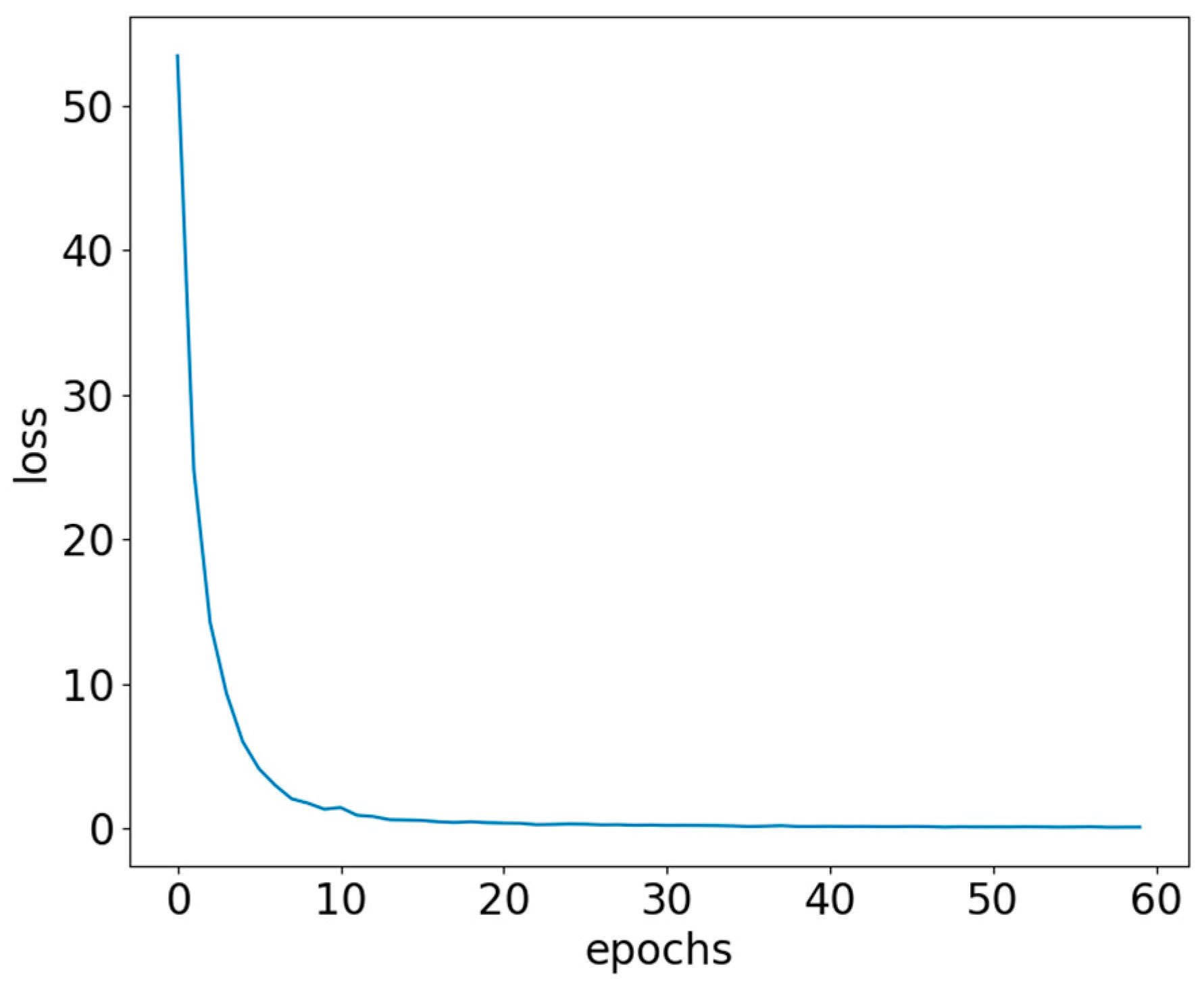
The above steps are used to train the CNN model and keep optimizing the model parameters through step 3. The loss values of the model as the number of model training times (epochs) increases are shown in Figure 13.
As can be seen in Figure 13, the model parameters stabilize after more than 15 epochs. Therefore, recognition performance is subsequently validated on the test set using these stable parameters and the results are plotted as a confusion matrix. Further, these results are compared with the performance of the VGGNet model and the Resnet model. The results of the confusion matrix are shown in Figure 14.
The recognition results of the test set are displayed in the confusion matrix in Figure 14. As can be seen from the figure, the VGGNet model and the Resnet model have significantly more recognition error results than the CNN used in this paper. Despite the better performance of the CNN used in this paper, two mixed signals are still misidentified as rain clutter. The reason for this analysis may be due to the excessive energy of the rain clutter, which leads to recognition errors. By comparing the computational metrics and training time for 20 epochs in Table 4, it can be seen that the CNN model used in this paper outperforms the VGG network and the Resnet network in most of the metrics. Therefore, it can be concluded that the modified CNN is significantly better than the VGG network and the Resnet network in terms of recognition accuracy. Therefore, the modified CNN will be selected for subsequent practical applications.

5. Application to Anti-Rain Clutter

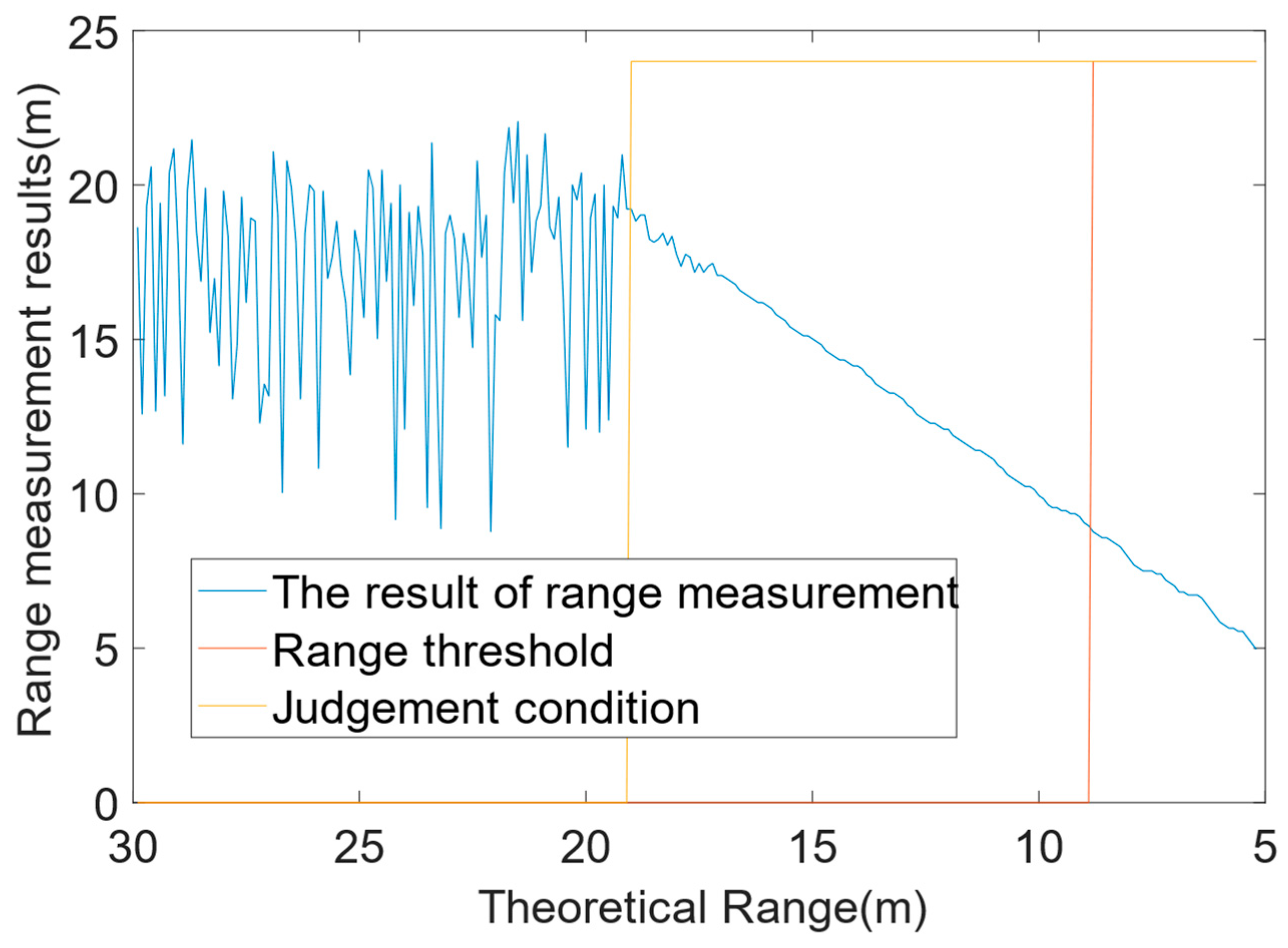
After determining the optimal parameters of the model, it was applied to the ranging measure task of the triangular wave linear frequency modulation detector in the rainfall environment. The echo signal received by the detector was recognised. When the recognition result was rain clutter, the signal was not subjected to the ranging measure process; conversely, when the recognition result showed that the signal contains the target signal, the signal was ranged. The ranging measure results after anti-interference processing are shown in Figure 15. When the signal is recognized as containing the target signal five times in a row, it is judged that the target is already within the detection range of the detector which is reflected in the figure as yellow lines.
When the CNN model recognised the echo signal from the triangular wave linear frequency modulation detector as a rain clutter signal, the system did respond to the signal. Specifically, the system did not output the range threshold before the yellow line in Figure 15, and started outputting the range threshold only after the yellow line judgement condition. As can be seen from the results, the system successfully and correctly outputs the range threshold at nine meters. This validates the effectiveness of using the recognition method for anti-rain clutter.

6. Conclusions

The purpose of this paper is to investigate the anti-interference method of millimeter-wave radar in severe weather environments such as rainfall environments. The influence of a rainfall environment on the millimeter-wave radar signal is studied based on the electromagnetic simulation by CST. Subsequently, according to the effect of the rainfall environment on the signal, we complete the signal detection model under the rainfall environment and conduct a simulation of the echo signal for the CNN model dataset production. We then combine this with experimental measurements to study the rainfall environment on the triangular wave linear frequency modulation detector ranging performance and use the CNN recognition to classify the echo signal. Ignoring the results of rain clutter signals, we then start the output of the distance threshold when it is in the part that contains the target signal. The recognition results of the CNN network are compared with VGGnet. The comparative analysis validates the accuracy of the CNN model used in this paper. The final results validate the effectiveness of using the CNN model in this paper to classify signals in a rainfall environment for anti-interference effects. This study provides new ideas and solutions for an anti-interference method for millimeter-wave radar when it faces interference from a bad weather environment, which is important for improving the anti-interference capability of radar systems. At the same time, this study also provides a valuable reference for future related research and promotes further in-depth discussion and development of anti-interference technology.

Author Contributions

Conceptualization, C.Z. and S.Z.; methodology, C.Z. and S.Z.; software, C.Z.; validation, C.Z., C.S. and S.C.; formal analysis, C.Z. and C.S.; resources, S.Z. and S.C.; data curation, C.Z. and C.S.; writing—original draft preparation, C.Z.; writing—review and editing, S.Z. and S.C.; visualization, C.Z.; supervision, S.Z.; project administration, S.Z.; funding acquisition, S.Z. and S.C. All authors have read and agreed to the published version of the manuscript.

Funding

This work was supported in part by the National Natural Science Foundation of China (NSFC) under grant 62271261, grant 61971226 and grant 62301252; and Fundamental Research Funds for the Central Universities under grant 30922010717.

Data Availability Statement

The data presented in this study are only available on request from the corresponding author due to privacy restrictions.

Acknowledgments

The authors would like to thank the anonymous reviewers for their careful assessment of our work.

Conflicts of Interest

The authors declare no conflicts of interest.

References

  1. Tan, B.; Ma, Z.; Zhu, X.; Li, S.; Zheng, L.; Chen, S.; Huang, L.; Bai, J. 3-D Object Detection for Multiframe 4-D Automotive Millimeter-Wave Radar Point Cloud. IEEE Sens. J. 2023, 23, 11125–11138. [Google Scholar] [CrossRef]
  2. Futatsumori, S.; Shibagaki, N. 96 GHz Millimeter-Wave Radar System for Airport Surface Detection Purpose. In Proceedings of the 2022 IEEE Conference on Antenna Measurements and Applications (CAMA), Guangzhou, China, 14–17 December 2022; IEEE: Piscataway, NJ, USA, 2022; pp. 1–2. [Google Scholar]
  3. Zhang, Z.; Qiu, Z.; Hu, W.; Lu, Y.; Zheng, W. Research on Wingtip Distance Measurement of High-Speed Coaxial Helicopter Based on 77 GHz FMCW Millimeter-Wave Radar. Meas. Sci. Technol. 2023, 34, 085111. [Google Scholar] [CrossRef]
  4. Gharamohammadi, A.; Dabak, A.G.; Yang, Z.; Khajepour, A.; Shaker, G. Volume-Based Occupancy Detection for In-Cabin Applications by Millimeter Wave Radar. Remote Sens. 2024, 16, 3068. [Google Scholar] [CrossRef]
  5. Guan, J.; Yin, W.; Xia, Y.; Wang, L. A MIMO Millimeter-Wave Radar for High-Resolution Imaging. In Proceedings of the IET International Radar Conference (IRC 2023), Chongqing, China, 3–5 December 2023; Institution of Engineering and Technology: London, UK, 2023; pp. 57–62. [Google Scholar]
  6. Shibly, I.H.; Zaman, M.M.; Hossain, M.S.; Hasan, M.M.S. Performance Analysis of Adaptive Cruise Control Using Frequency Modulated Continuous Wave Radar Under Rain Clutter. In Proceedings of the 2023 26th International Conference on Computer and Information Technology (ICCIT), Cox’s Bazar, Bangladesh, 13–15 December 2023; IEEE: Piscataway, NJ, USA, 2023; pp. 1–5. [Google Scholar]
  7. Wang, W.; Yang, G.; Zhang, Y. Application of Two-Dimensional Filtering in Rain Clutter Filtering. In Frontier Computing; Hung, J.C., Yen, N.Y., Chang, J.-W., Eds.; Lecture Notes in Electrical Engineering; Springer Nature: Singapore, 2022; Volume 827, pp. 1756–1761. [Google Scholar]
  8. Chen, K.; Zhang, J.; Chen, S.; Zhang, S.; Zhao, H. Recognition and Estimation for Frequency-Modulated Continuous-Wave Radars in Unknown and Complex Spectrum Environments. In IEEE Transactions on Aerospace and Electronic Systems; IEEE: Piscataway, NJ, USA, 2023; Volume 59, pp. 6098–6111. [Google Scholar]
  9. Chen, K.; Zhang, J.; Chen, S.; Zhang, S.; Zhao, H. Active Jamming Mitigation for Short-Range Detection System. In IEEE Transactions on Vehicular Technology; IEEE: Piscataway, NJ, USA, 2023; Volume 72, pp. 11446–11457. [Google Scholar]
  10. Lecun, Y.; Bottou, L.; Bengio, Y.; Haffner, P. Gradient-based learning applied to document recognition. In Proceedings of the IEEE; IEEE: Piscataway, NJ, USA, 1998; Volume 86, pp. 2278–2324. [Google Scholar]
  11. Krizhevsky, A.; Sutskever, I.; Hinton, G.E. ImageNet classification with deep convolutional neural networks. Commun. ACM 2012, 60, 84–90. [Google Scholar] [CrossRef]
  12. Simonyan, K.; Zisserman, A. Very Deep Convolutional Networks for Large-Scale Image Recognition. arXiv 2014, arXiv:1409.1556. [Google Scholar]
  13. He, K.; Zhang, X.; Ren, S.; Sun, J. Deep Residual Learning for Image Recognition. In Proceedings of the 2016 IEEE Conference on Computer Vision and Pattern Recognition (CVPR), Las Vegas, NV, USA, 27–30 June 2016; IEEE: New York, NY, USA, 2016; pp. 770–778. [Google Scholar]
  14. Tan, M.; Le, Q.V. EfficientNet: Rethinking Model Scaling for Convolutional Neural Networks. In Proceedings of the International Conference on Machine Learning, Long Beach, CA, USA, 9–15 June 2019; Chaudhuri, K., Salakhutdinov, R., Eds.; Jmlr-Journal Machine Learning Research: San Diego, CA, USA, 2019; Volume 97. [Google Scholar]
  15. Howard, A.; Sandler, M.; Chu, G.; Chen, L.-C.; Chen, B.; Tan, M.; Wang, W.; Zhu, Y.; Pang, R.; Vasudevan, V.; et al. Searching for MobileNetV3. In Proceedings of the 2019 IEEE/CVF International Conference on Computer Vision (ICCV 2019), Seoul, Republic of Korea, 27 October–2 November 2019; IEEE Computer Soc: Los Alamitos, CA, USA, 2019; pp. 1314–1324. [Google Scholar]
  16. Li, J.; Zhang, S.; Zhu, L.; Chen, S.; Hou, L.; Li, X.; Chen, K. Carrier-Free Ultra-Wideband Sensor Target Recognition in the Jungle Environment. Remote Sens. 2024, 16, 1549. [Google Scholar] [CrossRef]
  17. Strząbała, K.; Ćwiąkała, P.; Puniach, E. Identification of Landslide Precursors for Early Warning of Hazards with Remote Sensing. Remote Sens. 2024, 16, 2781. [Google Scholar] [CrossRef]
  18. Jiang, C.; Zhang, H.; Zhan, R.; Shu, W.; Zhang, J. Open-Set Recognition Model for SAR Target Based on Capsule Network with the KLD. Remote Sens. 2024, 16, 3141. [Google Scholar] [CrossRef]
  19. Dai, Y.; Yang, S.; Lee, K. Sensing and Navigation for Multiple Mobile Robots Based on Deep Q-Network. Remote Sens. 2023, 15, 4757. [Google Scholar] [CrossRef]
  20. Dang, X.; Fan, K.; Li, F.; Tang, Y.; Gao, Y.; Wang, Y. Multi-Person Action Recognition Based on Millimeter-Wave Radar Point Cloud. Appl. Sci. 2024, 14, 7253. [Google Scholar] [CrossRef]
  21. Jia, F.; Li, C.; Bi, S.; Qian, J.; Wei, L.; Sun, G. TC–Radar: Transformer–CNN Hybrid Network for Millimeter-Wave Radar Object Detection. Remote Sens. 2024, 16, 2881. [Google Scholar] [CrossRef]
  22. Bai, Y.; Wang, J.; Chen, P.; Gong, Z.; Xiong, Q. Hand Trajectory Recognition by Radar with a Finite-State Machine and a Bi-LSTM. Appl. Sci. 2024, 14, 6782. [Google Scholar] [CrossRef]
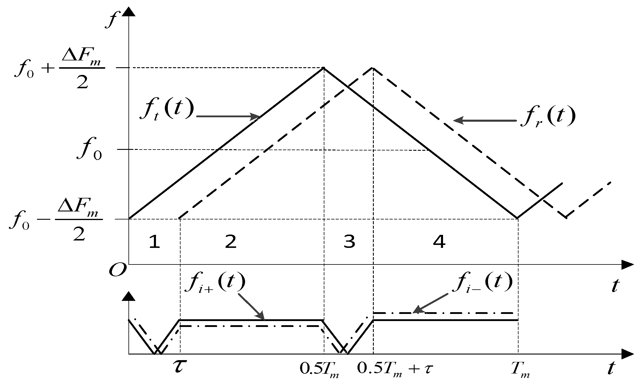
Figure 1. Schematic diagram of target detection using the triangular wave linear frequency modulation signal.
Remotesensing 16 03907 g001
Figure 2. Field experiment and result of range measurement. (a) Field experiment scene of range measurement. (b) Result of range measurement.
Remotesensing 16 03907 g002
Figure 3. CST simulation analysis. (a) Schematic diagram. (b) CST model diagram.
Remotesensing 16 03907 g003
Figure 4. Results of CST simulation analysis. (a) Result of point O. (b) Result of point P.
Remotesensing 16 03907 g004
Figure 5. Raindrop spectrum modeling under 1.2 rainfall rate.
Remotesensing 16 03907 g005
Figure 6. The results of simulation in rainfall environment. (a) Time-domain diagram. (b) Frequency-domain diagram. (c) Spectrogram.
Remotesensing 16 03907 g006
Figure 7. Signal detection experiment in the rainfall environment.
Remotesensing 16 03907 g007
Figure 8. The rain clutter signals collected from the experiment. (a) Time-domain diagram (b) Frequency-domain diagram. (c) Spectrogram.
Remotesensing 16 03907 g008
Figure 9. Range measurement experiment under a rainfall environment. (a) Schematic diagram. (b) Scene. (c) Range measurement results.
Remotesensing 16 03907 g009
Figure 10. The spectrograms under different environmental and signal conditions from the experiment. (a) The target signal in a non-rain environment. (b) The rain clutter signal in a rain environment. (c) The mixed signal in a rain environment.
Remotesensing 16 03907 g010
Figure 11. The spectrograms under different environmental and signal conditions from the simulation after performing thresholding. (a) The target signal in a non-rain environment. (b) The rain clutter signal in a rain environment (c) The mixed signal in a rain environment.
Remotesensing 16 03907 g011
Figure 12. The structure of the CNN.
Remotesensing 16 03907 g012
Figure 13. The loss of the CNN model.
Remotesensing 16 03907 g013
Figure 14. The results of the confusion matrix under different CNN models. (a) The confusion matrix under the VGGnet model. (b) The confusion matrix under the Resnet model. (c) The CNN confusion matrix under the model used in this paper.
Remotesensing 16 03907 g014
Figure 15. The ranging result after recognition.
Remotesensing 16 03907 g015
Table 1. The k H , k V , α H , and α V parameters for 24 GHz and 35 GHz .
f k H k V α H α V
24 GHz 0.14250.14041.01010.9561
35 GHz 0.33740.32240.90740.8761
Table 2. The simulated detector parameters.
f Δ F m T m f S
24   GHz 300   MHz 8   μ s 100   MHz
Table 3. The structural parameters of the CNN.
The Output Image DimensionsWeights Bias
Input 3 × 224 × 224 00
Gray 1 × 224 × 224 00
Convolution 220 × 220 × 30 75030
ReLU1 220 × 220 × 30 00
Maxpooling 55 × 55 × 30 00
Affine1 1 × 1 × 100 9,075,000100
ReLU2 1 × 1 × 100 00
Affine2 1 × 1 × 3 3003
Table 4. The metrics of the model performance on the test set under different models.
VGGnetResnetCNN of This Paper
MixRainTargetMixRainTargetMixRainTarget
Precision0.9380.9470.9920.9860.9130.9960.9840.9881.0
Recall0.9380.9510.9880.9010.9881.00.9880.9841.0
Specificity0.9690.9730.9960.9940.9530.9980.9920.9941.0
Time(s)101,988.785022.14260.67
Disclaimer/Publisher’s Note: The statements, opinions and data contained in all publications are solely those of the individual author(s) and contributor(s) and not of MDPI and/or the editor(s). MDPI and/or the editor(s) disclaim responsibility for any injury to people or property resulting from any ideas, methods, instructions or products referred to in the content.