Abstract
Sea ice is a crucial component of the global climate system. The China–French Ocean Satellite Scatterometer (CFOSAT/SCAT, CSCAT) employs an innovative rotating fan beam system. This study applied principal component analysis (PCA) to extract classification features and developed an ensemble machine learning approach for sea ice detection. PCA identified key features from CSCAT’s backscatter information, representing outer and sweet swath observations. The ensemble model’s performances (OA and Kappa) for the Northern and Southern Hemispheres were 0.930, 0.899, and 0.844, 0.747, respectively. CSCAT achieved an accuracy of over 0.9 for close ice and open water but less than 0.3 for open ice, with misclassification of open ice as closed ice. The sea ice extent discrepancy between CSCAT and the National Snow and Ice Data Center (NSIDC) was −0.06 ± 0.36 million km2 in the Northern Hemisphere and −0.03 ± 0.48 million km2 in the Southern Hemisphere. CSCAT’s sea ice closely matched synthetic aperture radar (SAR) imagery, indicating effective sea ice and open water differentiation. CSCAT accurately distinguished sea ice from open water but struggled with open ice classification, with misclassifications in the Arctic’s Greenland Sea and Hudson Bay, and the Antarctic’s sea ice–water boundary.
1. Introduction
Sea ice is a mixture of ice crystals, air bubbles, and brine formed in seawater. It covers approximately 7–15% of the world’s oceans and is one of the most important components of the cryosphere. Sea ice influences the global ocean radiative flux balance [1], thermohaline circulation [2], biogeochemical cycles [3], and polar navigation and operations [4], as one of the global cold sources. The increase in global temperature in recent decades has led to significant changes in polar sea ice. Satellite records suggest that the extent of Arctic sea ice has repeatedly reached record lows [5], while the extent of Antarctic sea ice varies greatly, experiencing periods of positive trends and maxima of sea ice extent [6,7,8]. However, it has also reached record lows in recent years [9]. This change in sea ice triggers several global impacts, such as changes in marine ecosystems, atmospheric circulation, and Arctic warming [10]. Therefore, it is important to monitor the distribution of sea ice in the polar regions.
Microwave remote sensing is widely used due to its capabilities for weather-independence, all-day observation, long-term monitoring, and comprehensive coverage [11]. In particular, satellite scatterometers have attracted attention as an active microwave remote sensing system that operates without imaging capabilities. These systems are crucial for providing real-time, accurate parameters of sea ice by emitting microwave pulses towards the Earth’s surface and analyzing the backscattered signals to infer surface properties. Table 1 provides a comprehensive compilation of various microwave scatterometer systems along with relevant bibliographic references, demonstrating their application in sea ice monitoring by several international agencies. It is noteworthy that these scatterometers predominantly work in the C-band (5.3 GHz) and Ku-band (13.5 GHz) frequencies. Based on their beam system, they are further classified into fixed fan beam, rotating pencil beam, and rotating fan beam scatterometers. Based on polarization, these systems are differentiated into vertical polarization (VV) and horizontal polarization (HH). The European Space Agency (ESA) is leading the advancement of C-band single polarized scatterometers with fixed fan beam, particularly through the development of instruments such as the Active Microwave Instrument-Scatterometer (AMI-SCAT) and Advanced Scatterometer (ASCAT). On the other hand, the National Aeronautics and Space Administration (NASA) focused more on Ku-band dual-polarization scatterometers. This technology has evolved significantly, moving from early fixed fan beam scatterometers (such as SeaSat-A Scatterometer System, SASS, and the NASA Scatterometer Satellite, NSCAT) to advanced rotating pencil beam scatterometers (such as SeaWinds and RapidScat). In addition to ESA and NASA, India and China have also made commendable progress in this field through the independent development of the Oceansat Scatterometer (OSCAT) and HY-2 Scatterometer (HSCAT). These systems are comparable to NASA’s SeaWinds in terms of frequency, polarization, and beam system. A notable milestone was reached in 2021 with the launch of the Chinese–French Oceanography Satellite (CFOSAT), a collaborative project between China and France that carries the innovative Chinese-French Ocean Satellite Scatterometer (CSCAT)—a Ku-band dual polarization rotating fan beam scatterometer. To further expand this range of instruments, China’s FY-3E satellite was deployed in 2022, equipped with Wind Radar (WindRad), which uses dual-frequency and dual-polarization. This deployment is particularly notable, as it marks the first use of horizontal C-band polarization in Earth observation [12], signifying a new chapter in the microwave remote sensing of sea ice.
Satellite scatterometers can provide daily observations of polar regions and are commonly used to map the extent of sea ice. Table 1 lists retrieval algorithms used for sea ice detection related to satellite scatterometers, which are broadly divided into two groups. The first group is called the Remund/Long-NSCAT (RL-N) algorithm, which uses linear discriminant analysis to classify ice and water by constructing features such as polarization ratio and frequency ratio [13]. The versatility of the RL-N algorithm is evident in its application to data from a variety of scatterometers, including OSCAT, HSCAT, and CSCAT, among others. These results show good consistency with sea ice concentration. However, the method has certain limitations; the accuracy of the RL-N algorithm can be significantly affected by wind-induced surface roughness and summer ice melt [14]. These effects need to be mitigated in the post-classification process by employing binary image processing techniques and sea ice growth/retreat constraint methods [15,16]. The second group refers to the Royal Netherlands Meteorological Institute (KNMI) algorithm proposed by the Royal Netherlands Meteorological Institute. This algorithm is designed for the analysis of sea ice using AMI-SCAT data and introduces geophysical model functions (GMFs) for sea ice detection. It contains Bayesian classifiers that are used to determine sea ice, as described by de Haan and Stoffelen [17] and Verspeek [18]. This approach has been successfully applied to satellite data from SeaWinds, ASCAT, HSCAT, and CSCAT. These GMFs for different sensors exhibit unique characteristics. AMI-SCAT’s GMF describes sea ice probability using an ice cone line in the three-dimensional σ0 space, assuming isotropic backscattering [17,18]. ASCAT’s GMF is based on a linear relationship between the forward, mid, and aft beams, with sea ice backscatter characteristics changing with incidence angle [19]. SeaWinds’ GMF represents sea ice properties through a linear relationship between vertically and horizontally polarized signals [20]. CSCAT, on the other hand, uses a look-up table to define the GMF due to the complex observation model [21]. This validation indicates that the method provides more accurate information for characterizing sea ice during the melting season. The GMFs have strong dependency on specific types of remote sensors, which can impose significant limitations when adapting to data from other sensor types or platforms.
It is worth noting that the introduction of new rotating fan beam systems such as CSCAT and WindRad introduces variability in incidence and azimuth angles, which has a significant impact on backscatter from OW and sea ice surfaces [22]. To deal with the complexity that arises from multiple angles of incidence and azimuth, the RL-N and KNMI algorithms have also been adapted for use with the CSCAT. Zhai et al. [23] addressed this problem by calculating the polarization ratio using the average of the horizontal and vertical polarization CSCAT backscatter coefficients over angles of incidence and azimuth. However, directly calculating the polarization ratio may reduce the detection accuracy because sea ice and seawater have different sensitivities to incidence and azimuth angles. At the same time, the CSCAT GMF model was first introduced in CSCAT by Liu et al. [24], which simplified the problem of mixed geometry observations by selecting backscatter observations near a 40° incidence angle to build a geophysical model of sea ice. The method of selecting a 40° incidence angle reduces the rotating fan beam system to a rotating pencil bean system. Li et al. [21] proposed a method of creating an incidence angle lookup table to construct a GMF to solve the problem of mixing incidence and azimuth observations. They observed a large standard deviation between the lowest and highest incidence angles when constructing a look-up table model, and therefore truncated the observations at both incidence angles. Moreover, the linear relationship between the incidence angle and the backscatter coefficient has also been used to correct this effect [13,25]. In essence, polarization ratio, frequency ratio, and normalization coefficients are still unable to fully mitigate the errors caused by wind-induced sea surface roughness. For CSCAT, with its multi-angle observations, the construction of GMFs is significantly more complex than traditional three-dimensional spatial distributions. It can no longer be expressed using a simple three-dimensional mathematical formula and instead requires a lookup table for implementation. Principal component analysis (PCA), traditionally viewed as a downscaling method, serves a dual role: It reduces the dimensionality of the feature space and highlights uncorrelated features [26,27]. Previous studies used PCA in sea ice retrieval by combining passive microwave radiometers and scatterometers [28] and have showed that it is effective in reducing the complexity of feature space and improving sea ice classification efficiency. However, the application of PCA to scatterometer observations for classification feature extraction has not been studied. This represents an opportunity for novel research that could potentially affect the accuracy of sea ice detection using scatterometer data.
The study aims to (1) extract classification features from CSCAT observations using PCA, (2) build an ensemble machine learning model to detect sea ice in both the Northern and Southern Hemispheres, and (3) validate the results of CSCAT sea ice detection by comparing with similar types of sea ice products and assessing the validity and feasibility of the developed model. As such, this paper not only eliminates the dependency on specific functions through the use of PCA, but also presents an automated algorithmic framework that requires no empirical parameters or manual identification, making it versatile enough to be applied across various scatterometer platforms.

Table 1.
Representative microwave scatterometer system and related references for sea ice application from various agencies in different countries (modified based on Long [29]).
Table 1.
Representative microwave scatterometer system and related references for sea ice application from various agencies in different countries (modified based on Long [29]).
| Sensor | Agency | Frequency | Polarization | Reference | Mission | Dates |
|---|---|---|---|---|---|---|
| SASS | NASA | Ku | 2VV*2 2HH*2 | Yueh et al. [30] | SeaSat | 1978.06–1978.10 |
| AMI-SCAT | ESA | C | 3VV | Verspeek [18] 2 de Haan and Stoffelen [17] 2 | ERS-1 | 1991.07–1996.07 |
| ERS-2 | 1995.04–2001.01 | |||||
| NSCAT | NASA | Ku | 3VV*2 1HH*2 | Remund and Long [13] 1 | ADEOS | 1996.09–1997.06 |
| SeaWinds | NASA | Ku | HH-inner VV-outer | Belmonte Rivas and Stoffelen [20] 2 | ADEOS-2 | 2002.12–2003.10 |
| QuikSCAT | 1999.06–2009.11 | |||||
| ASCAT | ESA | C | 3VV*2 | Belmonte Rivas et al. [19] 2 Breivik et al. [31] 2 Lindell and Long [32] 2 Aaboe et al. [33] 2 | Metop-A | 2006.10–2021.11 |
| Metop-B | 2012.09– | |||||
| Metop-C | 2018.11– | |||||
| OSCAT | ISRO | Ku | HH-inner VV-outer | Hill and Long [34] 1 | OceanSat-2 ScatSAT-1 | 2009.09–2014.02 2016.09–2021.02 |
| HSCAT | NSOAS | Ku | HH-inner VV-outer | Xu et al. [35] 1 Li et al. [16] 1 Zou et al. [36] 1 | HY-2A | 2011.08–2022.04 |
| HY-2B | 2018.10– | |||||
| HY-2C | 2020.09– | |||||
| HY-2D | 2021.05– | |||||
| RapidScat | NASA | Ku | VV HH | Singh et al. [28] 1 | ISS RapidScat | 2014.09–2016.08 |
| CSCAT | CNSA | Ku | VV HH | Liu et al. [24] 2 Zhai et al. [23] 1 Li et al. [21] 2 Liu et al. [37] 2 Xu et al. [38] 1 | CFOSAT | 2018.10–2023.01 |
| WindRAD | CMA | C/Ku | VV*2 HH*2 | Zhai et al. [39] 1 | FY-3E | 2021.05– |
1 Algorithm belonging to RL-N. 2 Algorithm belonging to KNMI.
2. Materials and Methods
2.1. Materials
2.1.1. Input Data
The CSCAT Level 2A (L2A) products used here were maintained by the National Satellite Ocean Application Service, can be derived from https://osdds.nsoas.org.cn, accessed on 21 January 2023, and cover the period 2019–2022. CSCAT on-board CFOSAT is a real aperture radar operating in the Ku band (13.256 GHz) and collects vertical (VV) and horizontal (HH) polarization backscatter coefficient from two rotating fan beam antennas (Figure 1). The CSCAT covers a 1050 km swath divided into 25 km and 12.5 km regular grid wind vector cells (WVCs), with incidence angles ranging from 25° to 48° for fan beams. For the objectives of this study, the 25 km resolution provides sufficient detail and accuracy, while also demonstrating good quality and stability in our study area, making it the most suitable choice for this research. WVCs for cross-track orbit near ~43°S are shown in Figure 1c. According to Li et al. [40], the WVCs can be classified into three groups: outer swath WVCs (number 1–5, number 38–42); sweet swath WVCs (number 6–12, number 31–37); and nadir swath WVCs (number 13–30). CSCAT provides multiple views in the Ku band and per WVC, with a smaller number of views and less azimuth diversity in the outer and nadir swath and a larger number of views and more azimuth diversity in the sweet swath [41]. The incidence angle of WVCs exhibits axisymmetric properties relative to the nadir point and shows a large range of variability as the nadir point is approached. The azimuth angle shows central symmetry with respect to the nadir point. This characteristic distribution is displayed in Figure 1b and was a direct consequence of the rotating fan beam system of the CSCAT. It represented the forward- or backward-looking wind. The design of CSCAT cleverly combined the features of fixed fan beam and rotating pencil beam scatterometers. This combination not only expanded the swath, but also significantly increased the diversity of observation geometries within a specific swath.
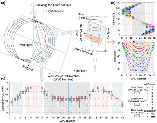
Figure 1.
(a) Observation geometry of CSCAT adapted from Zhang et al. [42]. (b) Incidence and azimuth angles versus the cross-track wind vector cell (WVC) number for a row at a latitude of ~43°S from orbit observed on 1 January 2019 at 07:56:26, showcasing WVC views in color and and using symbolic circles and forks, respectively. (c) The average number of views at WVC across the swath.
2.1.2. Auxiliary Data
Auxiliary data were needed for three different purposes, as outlined in Table 2. First, it was necessary for prior reference information. Second, it was required for validating the detection results. Finally, a static dataset was needed that was relevant to the polar grid projection and controlled the quality of the detection results.

Table 2.
Data used for research and model construction.
- Prior reference datasets
Scatterometer-based sea ice detection is essentially a supervised classification problem. The process relies on a high-quality reference dataset to train and validate the performance of the model. According to Ivanova et al. [43] and Kern et al. [44], hybrid algorithms provided the most reliable estimates of sea ice concentration for climate monitoring purposes. In this study, we used from the CMEMS Ocean and Sea Ice Thematic Assembly Centre (OSI TAC) global reprocessed sea ice concentration product as prior reference dataset, which is a redistribution of the European Organization for the Exploitation of Meteorological Satellites (EUMETSAT) OSISAF Climate Data Record (CDR), labelled OSI-450, and the Interim Climate Data Record (ICDR), labelled OSI-430-a. This dataset was derived from Scanning Multichannel Microwave Radiometer (SMMR), Special Sensor Microwave-Imager (SSM/I), and Special Sensor Microwave-Imager/Sounder (SSMIS) data and uses a hybrid, adaptive, and self-optimizing sea ice concentration algorithm, which is an extension and improvement of the bootstrap algorithm [45] and the Bristol algorithm [46]. The algorithm utilized three channels (∼19 GHz for vertical polarization and ∼37 GHz for horizontal and vertical polarization) to provide optimal accuracy in both open water and consolidated ice conditions. It was characterized by quantifiability, temporal consistency, and sustainability and was therefore suitable as a prior reference dataset compared to independent estimates of sea ice concentration in regions with extremely high and low ice concentrations [47]. To match the time series of CSCAT observations, we obtained records of daily sea ice concentration for the period from 1 January 2019 to 31 December 2022. The data were projected as Equal-Area Scalable Earth 2.0 Grids (EASE-Grid 2.0) with a spatial resolution of 25 km.
- 2.
- Comparison datasets
To ensure an independent evaluation beyond OSISAF sea ice concentration, we introduced two additional datasets for third-party comparison, which allowed us to compare scatterometer and microwave radiometer sea ice cover results. Two similar sea ice products were used for spatial comparisons at a given time. As one of the comparison data sets, the study used the near real-time sea ice edge products from OSISAF of the EUMETSAT. These sea ice edge was derived from atmospherically corrected SSMIS brightness temperatures and ASCAT backscatter values through a Bayesian detection approach, which classified the data into open water (OW), open ice (OI), and close ice (CI) [31]. In addition, to validate the accuracy of the CSCAT sea ice extent detection results, sea ice concentrations from Nimbus-7 SMMR and DMSP SSM/I-SSMIS Passive Microwave Data Version 1 (hereinafter referred to as NSIDC sea ice concentration) [48] serves as an independent comparison dataset. This NSIDC dataset, generated from SSMIS brightness temperature data, used the established NASA Team (NT) algorithm developed by the Oceans and Ice Branch at NASA’s Goddard Space Flight Center (GSFC) [49]. The dataset provided a 25-km daily sea ice concentration for both polar regions from 26 October 1978 to 31 May 2022.
High-resolution images from Sentinel-1, part of European Space Agency (ESA) Copernicus program, were used for local visual validation. The Sentinel-1 constellation, consisting of Sentinel-1A and 1B, carries C-band Synthetic Aperture Radar (SAR) sensors, which provide reliable all-weather, day-and-night Earth observations. SAR images, known for their high resolution, have been widely utilized to validate scatterometer-based sea ice detection [50]. The analysis used Sentinel-1A/1B SAR Level-1, extra wide (EW) swath images in ground range-detected (GRD) mode with an approximate spatial resolution of 20 m × 40 m [51], to verify the CSCAT results over main areas of the Arctic and Antarctic.
- 3.
- Static datasets
The static dataset used in this study consists of polar grid area information [52] and a land-sea mask, that provides arrays of the area in millions, as well as a land-sea mask for the 25 km grid for the Northern and Southern Hemispheres, respectively.
To improve the accuracy of sea ice detection, the retrieval results here are quality controlled using effective ice mask data. Valid sea ice is defined as the likely presence of ice where it has existed in the past based on a 35-year climatology report. Among other things, the Arctic ice mask data was obtained from the US Ice Centre [53], which is a dataset based on Arctic sea ice charts and sea ice concentration data provided by the US National Ice Centre. It contains 12 files covering the maximum sea ice extent from 1972 to 2007, with each file representing each month of the year. The Antarctic-specific study determined the maximum monthly effective sea ice extent in Antarctica by analyzing daily climatological OSI-450 sea ice concentration data from 1978 to 2020 and counting pixels with sea ice concentrations greater than 0 over a period of 42 years.
2.2. Methods
This study used PCA and ensemble machine learning model to automate the detection of sea ice using Level-2A CSCAT data from 2019 to 2022. The sea ice detected using this technique was compared with sea ice concentrations derived from passive microwave data, the sea ice edge determined by passive microwave and active scatterometer data, and SAR data for specific regions. Figure 2 illustrates the workflow for sea ice detection. The first step involved preprocessing the Level 2A CSCAT time series data. This included checking the pixel quality of the land and rain flag, reprojection, regrinding from orbit to polar stereographic grid, and calculating the polarization ratio. The result was 8 views of , and (Figure 2a). PCA was then applied to those three scatterometer parameters. The main component that most closely suggested ice and water was chosen as the distinguishing feature (Figure 2b). Regions of interest around the Arctic and Antarctic were selected, where different ice/ocean classes’ characteristics are expected. Corresponding prior information on sea ice concentration data were spatially and temporally matched with CSCAT using nearest neighbor interpolation (Figure 2c). At the same time, the period length was compared and determined for statistical analysis. This was followed by sample selection, from which single and ensemble machine learning classifiers were used to distinguish sea ice, with 80% of the data trained and validated with the remaining 20%. A preliminary sea ice map was then created based on an ensemble model. In the final phase, the map was refined by applying valid ice masks to reduce misdetection noise (Figure 2d).
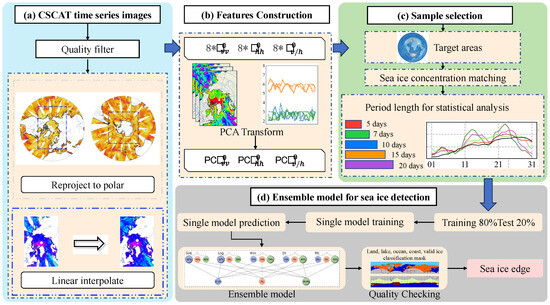
Figure 2.
Workflow of this study.
2.2.1. Features Construction
The satellite orbit data were projected to the Northern and Southern Hemispheres. This was process was conducted in order to minimize deformation and keep the poles at the center of the image when studying the polar regions. For this purpose, the NSIDC projection program was used (https://nsidc.org/data/user-resources/help-center/guide-nsidcs-polar-stereographic-projection, accessed on 30 January 2023). The CSCAT L2A data we used were derived from WVC’s orbit resampled data, recorded as backscattering (dB). During the polar projection process, we filtered out pixels that were labeled as land and affected by precipitation. The precipitation information used for this filtering came from the quality indicators in the L2B wind field retrieval data, specifically the rain_fail and rain_detect flags in the wvc_quality dataset. We then divided the data into the Northern and Southern Hemispheres based on latitude and longitude and excluded pixels within which the number of WVC views was zero. The CSCAT L2A orbit data were projected onto the poles, and then the projected data was interpolated using the radial interpolation function of the SciPy library in Python to ensure consistency of the orbital centers and sides with the observed number of views in the sweet swath and to produce the projected backscattered observation dataset:
where represents the WVC, represents the backscattering in vertical polarization for the WVC , and represents the backscattering in horizontal polarization for the WVC .
The polarization ratio was calculated according to WVC with the following equation:
A polar backscatter observation dataset was then constructed using the following equation:
This study selected the singular value decomposition method based on the Scikit-Learn library in Python [54]. PCA was then performed on the observations of datasets , to obtain the principal components of :
where represents the number of principal components, refers to the principal component of the vertical polarization, refers to the principal component of the horizontal polarization, and represents the principal component of the polarization ratio.
2.2.2. Dynamic Sampling
With the aim of obtaining representative samples of sea ice and seawater, training samples are crucial for sea ice detection. Microwave radiometric observations have revealed dynamic reference brightness temperatures of open water and sea ice (tie points) [55], demonstrating seasonal and interannual variability differences [56]. However, the seasonal and interannual variation of microwave scatter from open water and sea ice are not well understood. Currently, many methods for detecting sea ice using satellite scatterometers use a dynamic sample selection strategy or periodic model updates [34]. Liu et al. [57] collected 10 days of backscatter observations to build a lookup table for a dynamic sea ice geophysical model. The probability distribution function of open water and sea ice from OSI SAF was originally based on statistics from a fixed reference year (2007.3–2008.2) [31]. The probability density function’s update frequency has gradually increased from monthly to 15 days [33]. Zhai et al. [23] also examined the effect of the length of the training sample period on the effectiveness of the model and found that the accuracy did not improve when the period of training sets exceeded 7 days. The length of the sampling period depends on the availability and accessibility of the referenced sea ice information. This information is typically obtained through various methods such as satellite remote sensing, buoy observations, and sensor measurements. Data can only be collected at specific time intervals, such as daily, weekly, or monthly. The choice of sampling period depends on the study methodology, data availability, and the need for reliable statistics. Therefore, it is necessary to analyze and determine the appropriate period length.
We used the daily CMEMS sea ice concentration climate dataset as prior reference. First, the daily CMEMS sea ice concentration climate dataset was converted to a projection plane consistent with CSCAT preprocessing in order to eliminate the impact of errors that may result from different projection systems and to ensure that the data remained consistent with the study area. For the Northern Hemisphere (Southern Hemisphere), the projections were converted from epsg6931 (epsg6932) to epsg3411 (epsg3412). According to the spatiotemporal matching principle, the eigenvalues of the principal component eigenvalues and the sea ice concentration were extracted from the regions of interest in the Northern and Southern Hemisphere, respectively (Figure 3, yellow blocks), to obtain the scattering properties and spatial distribution information of sea ice. In order to effectively detect sea ice, sea ice concentration was divided into less than 30% open water, 30%–70% open ice, or more than 70% close ice. Such a division clarified the different sea ice conditions and provided effective training examples for model training:
where represented the number of principal components selected, was the selected principal component of vertical polarization, was the selected principal component of horizontal polarization, was the selected principal component of the polarization ratio, and was the sample label determined by CMEMS, i.e., open water, open ice, or close ice. Microwave scattering from open water and sea ice exhibited different variation characteristics at seasonal and interannual scales, and these characteristics determined the selection of the sampling period in this study. For each specific day, we collected sea ice and open water samples from the last 5, 7, 10, 15, and 20 days (including the current day) to ensure a balanced and representative dataset. We combined five sample periods of 5, 7, 10, 15, and 20 days and analyzed the sample characteristics and model effects by constructing characteristic time series of open water, open ice, and close ice for the period 2019–2022, which were used for determination of the last sampling period.
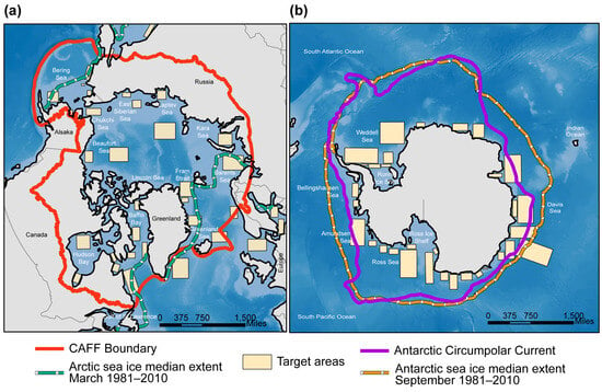
Figure 3.
Location map over (a) the Northern Hemisphere and (b) the Southern Hemisphere for the regions (marked in yellow colors) used in sample selection overlaid on the CAFF Boundary [58], Antarctic Circumpolar Current (https://data.aad.gov.au/dataset/4892/download, accessed on 20 March 2023) and sea ice median extent [59].
2.2.3. Single and Ensemble Model Construction
Ensemble methods combine the predictions of several base estimators built with a given learning algorithm in order to improve generalizability/robustness over a single estimator. More generally, ensemble models can be applied to any base learner for the purposes of averaging methods such as bagging methods, model stacking, or voting, or boosting methods, such as in AdaBoost. We chose the average voting classifier as the ensemble model. The average voting ensemble model is a machine learning technique that combines multiple base estimators. Specifically, it computes the predicted probabilities for each class from each base estimator and then averages these probabilities. The final class prediction is made based on the class with the highest average probability. Such a classifier can be useful for a set of equally well-performing models in order to balance out their individual weaknesses.
In this study, we selected five base estimators: Gaussian naive Bayes (Gnb), logistic regression (Log), K-nearest neighbors (Knn), decision tree (Dt), and random forest classifier (Rfc) to build an ensemble learning model for sea ice detection in the Northern and Southern Hemispheres. The training process of the ensemble model (Figure 4) was as follows: (1) The training and testing datasets were calculated based on the period length determined in the previous section. To ensure unbiased estimates, we divided the dataset into an 80% training set and a 20% testing set. (2) During model training, careful parameter tuning was performed to optimize the performance of each model. RandomizedSearchCV from the sklearn library was used to optimize the hyperparameters for each model. A 10-fold cross-validation approach assessed model performance, with 50 random hyperparameter combinations being sampled in order to identify the best configuration. The scoring = ‘f1’ metric was chosen to provide a comprehensive evaluation by considering both precision and recall. (3) After training, the probabilities predicted by each estimator were calculated for each class. That is, Gnb, Log, Knn, Dt, and Rfc generated probability maps for open water, open ice, and close ice, respectively. Specifically, the Gnb model computed the posterior probability by multiplying the conditional probability with the class prior probability. The Log model derived the class probability distribution through maximum likelihood estimation. The Knn model determined the classification probability based on the proportion of the nearest neighbors’ classes. The Dt model calculated the class probability at the leaf node based on the proportion of samples in each class. Finally, the Rfc averaged the predicted probabilities across multiple decision trees to produce the final class probabilities. After obtaining the probabilities for open water, open ice, and close ice, the class with the highest probability was selected as the final classification for that pixel. (4) Then, the predicted probabilities of all classifiers were averaged to obtain the probability maps for open water, open ice, and close ice. The final prediction was based on the class with the highest probability.
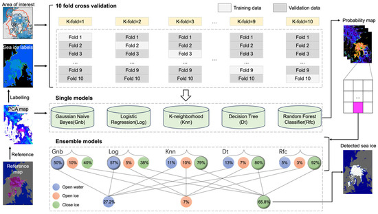
Figure 4.
Model structure of the soft voting ensemble learning and training process.
2.2.4. Accuracy Assessment
To verify accuracy of models, we used 20% of the test samples to construct a confusion matrix. This yielded various validation parameters, such as user accuracy (UA), producer accuracy (PA), overall accuracy (OA), the F1 score (F1), and the kappa coefficient (Kappa).
3. Results
After reviewing the L2 orbit data and daily projected data, there were a total of 116 days where CSCAT data was unusable. Specifically, 50 days of Level 2A orbital observations were missing, and 66 days were eliminated due to quality control measures (e.g., removal of invalid values, rain-affected pixels, and land pixels). Additionally, since we needed to collect samples from the past 5 consecutive days, a total of 22 days were affected due to insufficient sample sizes. The specific relevant data and reasons for deletion are listed in the Table 3. No sea ice forecasts were made in the study for these 138 data days. The number of days used for statistical analysis was 90%.

Table 3.
The list of invalid dates and reason for removal from statistical analysis from 1 January 2019 to 31 December 2022.
3.1. Characteristics of CSCAT Features
The CSCAT data included eight VV polarization (), eight HH polarization (), and eight polarization ratios (). There were obvious correlations between the properties of these observations. Figure 5a,b show the Pearson’s correlation for these observations in the Northern and Southern Hemisphere, respectively. As can be seen from the figures, there was not only a high correlation between adjacent (or ), but also a correlation between the set of and for each WVC. We applied PCA to the CSCAT polar backscatter observation dataset and assigned it to fewer principal components. With the bivariate plots of the principal component analysis (Figure 5c,d), we found that among the eight WVCs, the contributions of WVCs in views 3, 4, and 8 were more significant in and . In comparison, the results of view 8 showed a significant deviation from the results of views 3 and 4. Views 3 and 4 primarily occupied the outer swath and nadir swath, respectively. The WVCs of the nadir swath were characterized by azimuth angles of 0/360 or 180 degrees, corresponding to the forward and backward perspectives, accompanied by a wide range of incidence angles. Conversely, the WVCs in the outer swath were defined by azimuth angles of approximately 90 or 270 degrees, indicating lateral viewing angles, again with a wide range of incidence angles. View 8 was consistently located in the region designated the sweet swath, characterized by significant variability in the antenna’s azimuth angle. According to Li et al. [40], the WVCs in the sweet swath were the optimal area for measuring sea surface wind. Likewise, the WVCs of the sweet swath in the principal component analysis occupied a larger amount of information. Therefore, the first two principal components of and effectively characterized the observed information in the outer swath, nadir swath, and sweet swath. In contrast, the bivariate plot of shows that the first two principal components could only represent the outer swath, suggesting that the amount of information gathered using only the first two principal components accounted for almost 50% of the total observations. Spatial distribution analyses of the first four (out of eight) principal components conducted on 10 January 2019 for both the Northern and Southern Hemispheres (as shown in Figure 6a,b), revealed that the importance of and was mainly concentrated within the first two components. Meanwhile, the significance of the VH polarization was evenly distributed across all four components.
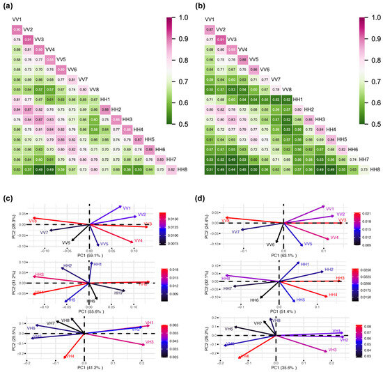
Figure 5.
Pearson’s correlation coefficients in the (a) Northern Hemisphere and (b) Southern Hemisphere and related principal component analysis (PCA) bioplots of CSCAT backscatter observations over the (c) Northern and (d) Southern Hemispheres on 10 January 2019.
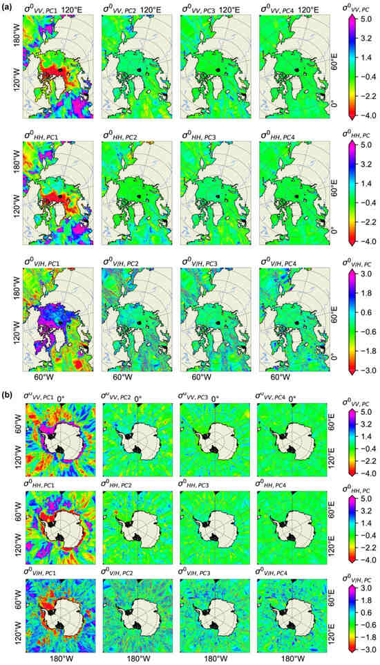
Figure 6.
Spatial distribution of the first four (out of eight) principal components of , and and polarization in the (a) Northern Hemisphere and (b) Southern Hemisphere on 10 January 2019, respectively.
Figure 7 shows the daily variation curves for the contributions of the first two principal components of and and the first four principal components of . These results suggested that the choice of the first two principal components for () polarization accounted for over 80% of the total variance explained, while the choice of the first four principal components for explained more than 65% of the total variance.
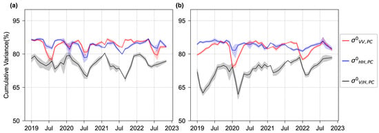
Figure 7.
Time series of cumulative variance of the eigenvalues for principal components in the (a) Northern and (b) Southern Hemispheres between 2019 and 2022.
3.2. Period Choice for Dynamic Sampling
Figure 8 presents the statistical averages of the first principal component of in both the Northern and Southern Hemispheres using different sampling periods of 5, 7, 10, 15, and 20 days. The analysis shows that shorter sample periods result in significant noise in the first principal component of the VV polarization, thereby enhancing contrast during seasonal variations. Conversely, extending the sampling period results in a smoother curve for the first principal component feature of VV polarization, suggesting a diminishing emphasis on seasonal variations. Subsequent comparisons of the detection performance of the random forest model were performed for the Northern and Southern Hemispheres in January–March and June–August, respectively, over the same range of sampling periods (5, 7, 10, 15, and 20 days). Table 4 presents the F1 scores for five different models across various sampling periods It highlights which sampling period (e.g., 5 days, 7 days, etc.) resulted in the highest F1 scores for each model. The table summarizes a total of 10 statistical scenarios, with 8 scenarios showing that the 5-day sampling period consistently achieved the highest F1 score.
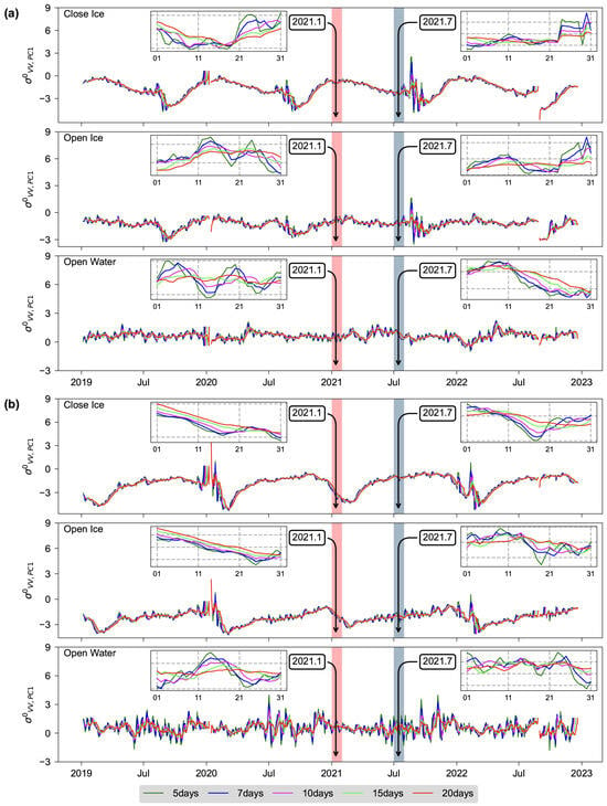
Figure 8.
Time series of with different period lengths in the (a) Northern Hemisphere and (b) Southern Hemisphere for close ice, open ice, and open water.

Table 4.
Period with the highest average F1 scores for each model (Dt, Gnb, Knn, Log, and Rfc) in the Northern and Southern Hemispheres.
After comprehensive evaluation, a sample period of 5 days was chosen for the dynamic sample statistics. Taking into account the possibility of incomplete sampling periods due to missing observations on certain dates, a forward search was performed to find available data no longer than 5 days. If the forward search exceeded 20 days, then dynamic sample data were considered missing on that date, and no modeling or sea ice detection was performed for that day.
3.3. Assessment for Single and Ensemble Models
In this study, five individual models were modelled: Gnb, Log, Knn, Dt, and Rfc. The variable importance of these models was assessed during the model building process, and cross-validation of F1 scores was performed to provide insight into the performance of the models and the relative importance of each feature. Variable importance is an important measure of how strongly features influence the predictive power of a model. We assessed feature importance using different metrics tailored to each model. For Dt and Rfc, Gini importance was used, which reflects the reduction in contamination by each feature. For Log and Gnb, feature weights from regression coefficients were used, with the magnitude of the coefficients indicating feature influence, and although Knn does not directly indicate feature importance, it can be assessed indirectly via model performance or weighted configurations.
Figure 9a shows the feature importance of these five models for the Northern and Southern Hemispheres. There are some differences in how different models rank for feature importance. Different models assigned different levels of importance to features. The most important feature was the first principal component of HH polarization. The ranking of and varied between the models: They took second and third place in Log-ranked third and second in others The situation in the Southern Hemisphere was more complex, as there were significant differences in the order of feature importance among models. In the Dt, Knn, and Rfc models, was the most important feature, while in the Gnb model, was the most important, and in the Log model, was the most important. This reflected the geographical differences between the Northern and Southern Hemispheres and the different responses to polarization features. Consequently, the models also showed variations in the ranking of radar polarization features for different regions. Figure 9b summarizes the distribution of F1 scores across the models during a 10-fold cross-validation period from 1 January 2019 to 31 December 2022. The F1 scores, which ranged from 0.660 to 0.750 for both hemispheres, indicated a commendable balance of precision and recall achieved by the models over the past four years. The Log model in the Southern Hemisphere showed the largest standard deviation (0.088), indicating greater variability in performance across different subsets compared to the other models. The standard deviations of the other models were between 0.028 and 0.069. Figure 9c shows the time series of F1 values obtained by 10-fold cross-validation for different machine learning models from 1 January 2019 to 31 December 2022. The Knn, Rfc, and ensemble models consistently showed relatively stable and high F1 values throughout both the Northern and Southern Hemispheres, indicating strong and sustained forecast performance in these regions. In contrast, Log showed larger fluctuations in F1 results and generally lower values, suggesting weaker and more unstable generalization abilities, especially in the Northern Hemisphere. For all models, there was no obvious temporal trend showing significant improvements or declines in F1 score over the analyzed period, suggesting stable model performance without noticeable deterioration or improvement. However, the different models showed differences in performance over the course of the season. Notably, in the Northern Hemisphere, the F1 score for all models increased continuously from July to September, and similarly, in the Southern Hemisphere, F1 scores were higher from January to March compared to other months. This pattern, observed continuously from 2019 to 2022, indicates that Ku-band CSCAT is particularly effective in identifying the melting status of sea ice during the summer months. On the other hand, the Log model outperformed Dt and Gnb in both hemispheres from January to March, but in the Southern Hemisphere, its F1 values were significantly lower than those of Dt and Gnb from July to September. The consistent performance of these models highlights their robustness and reliability in analyzing sea ice dynamics using radar polarization features, despite the inherent variability in environmental conditions between the Northern and Southern Hemispheres.
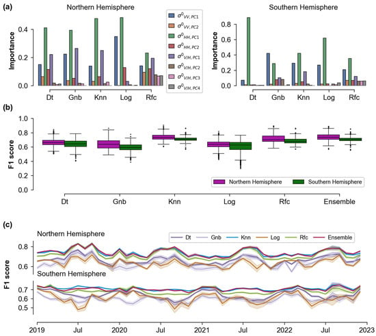
Figure 9.
(a) Feature importance for single models on 10 January 2019 in the Northern Hemisphere (left) and the Southern Hemisphere (right). (b) Statistical results of 10-fold cross-validation F1 scores for different machine learning models from 1 January 2019 to 31 December 2022. (c) Time series of 10-fold cross-validation F1 scores for different machine learning models from 1 January 2019 to 31 December 2022.
To evaluate the models, we summarized confusion matrices for individual and integrated models (Table 5). In both the Northern and Southern Hemispheres, the performance of the five individual models varied in different classification scenarios. For open water and close ice, Knn and Rfc achieved F1 values above 0.9, while the other three models also achieved values around 0.8. However, all five models had very low F1 values of less than 0.4 on open ice. Among them, Knn performed the best with an F1 value above 0.3, followed by Rfc in the Northern Hemisphere and Dt in the Southern Hemisphere. Among the results of five single models between 2019 and 2022, Knn and Rfc showed strong performance in the Northern Hemisphere, with F1 and OA values above 0.9 and kappa coefficients above 0.8, indicating high data consistency. In contrast, Dt, Gnb, and Log showed F1 and OA values between 0.7 and 0.9, with kappa coefficients ranging between 0.569 and 0.6887, reflecting moderate consistency. While Dt and Log had OA values around 0.7 in the Southern Hemisphere, Knn, Rfc, and Gnb reached OA values between 0.8 and 0.9. Only Knn and Rfc had kappa values above 0.7, indicating high model consistency, while Dt, Gnb, and Log had Kappa values below 0.6, indicating medium consistency. Overall, Knn and Rfc performed better than the other single models in terms of detection accuracy.

Table 5.
Summary of averaged detection accuracies through confusion matrix of sea ice edge classification in the Northern and Southern Hemisphere from 1 January 2019 to 31 December 2022.
In the Northern Hemisphere, the ensemble models slightly outperformed the best two individual models, Rfc and Knn, in terms of OA and Kappa values. Additionally, while the F1 score for open ice improved compared to Rfc, it still remained lower than that of Knn. A similar trend was observed in the Southern Hemisphere. The ensemble models showed a slight advantage over the best individual models in terms of OA and Kappa values. For open ice, the F1 score was higher than that of Rfc but still lower than Knn. Based on these observations, the ensemble models can be considered the preferred choice. Their overall performance, demonstrated by the improved OA and Kappa values, indicates their effectiveness in achieving better consistency and reliability across different scenarios. While KNN still outperforms the ensemble models in terms of F1 scores for open ice, the ensemble models’ superior overall performance suggests that they offer a more balanced and reliable solution across various classification tasks.
Figure 10 illustrates the time series of assessment parameters from 1 January 2019 to 31 December 2022. The overall classification metrics (OA and Kappa) had more similar daily trends to the UA, PA, and F1 values for close ice. However, these values were significantly lower from July to October in the Northern Hemisphere and from January to April in the Southern Hemisphere. UA, PA, and F1 values were generally higher in open water, with less seasonal variation and relatively low values, mainly in the Northern Hemisphere from January to April and in the Southern Hemisphere from April to October. The UA, PA, and F1 values for close ice and open water were higher than those for open ice. Figure 11 presents an error analysis based on the model classification confusion matrix, with the y-axis representing the misclassification rates for each class. Specifically, these rates were calculated by determining the number of pixels for each class (e.g., “Close Ice”, “Open Ice”, and “Open Water”) that were incorrectly classified as other classes and then dividing these misclassified pixel counts by the total number of pixels for that class. Error analysis showed that close ice was frequently mistakenly classified as open ice from July to October in the Northern Hemisphere and from January to April in the Southern Hemisphere, resulting in decreased classification accuracy. On the other hand, open water was frequently mistakenly identified as close ice from April to October in the Southern Hemisphere and January to April in the Northern Hemisphere, which also affected the accuracy of the classification. Furthermore, a significant portion of open ice was incorrectly identified as close ice, which helps to explain why close ice classification accuracy was typically lower.
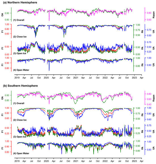
Figure 10.
The time series of the evaluation parameters for (1) overall, (2) close ice, (3) open ice, and (4) open water in the sea ice monitoring ensemble training model in the (a) Northern Hemisphere and (b) Southern Hemisphere from 1 January 2019 to 31 December 2022, respectively.
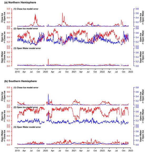
Figure 11.
Daily error analysis for (1) close ice, (2) open ice, and (3) open water in the sea ice monitoring ensemble training model in the (a) Northern Hemisphere and (b) Southern Hemisphere from 1 January 2019 to 31 December 2022, respectively.
3.4. Single and Ensemble Model-Based Sea Ice Mapping
This study used five single models and an averaged ensemble model for sea ice detection. The Northern and Southern Hemisphere sea ice detection results for 10 December 2019 and 10 June 2019 are shown in Figure 12. Each column represents origin reference SIC, classified reference SIC, and different models, namely Dt, Gnb, Knn, Log, and Rfc, from left to right. The reference map provided the observed sea ice distribution, serving as a comparison baseline. It is evident that the amount of sea ice was similar in both the Northern and Southern Hemispheres. There were differences between the models in terms of sea ice detection. The Knn and Rfc models overall performed better than the other models in classifying sea ice in both the Northern and Southern Hemispheres. The Knn model detected sea ice by calculating the distance between samples, while the Rfc model classified it by constructing a decision tree integration. These models might be better suited to the capture the spatiotemporal correlation of sea ice and dealing with its nonlinear features. Compared to the original reference maps, the Knn and Rfc single models tended to misclassify open ice as close ice at the sea ice boundary, whereas Dt and Log were more prone to misclassifying close ice as open ice. These differences were likely due to variations in the algorithmic principles and feature extraction functions. The advantage of Rfc and Knn lay in their overall robustness and stability for close ice, while Dt and Log demonstrated certain advantages in handling complex boundaries, particularly in distinguishing open ice from close ice.
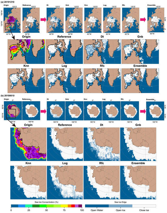
Figure 12.
Sea ice detection in the (a) Northern Hemisphere on 10 December 2019 and (b) Southern Hemisphere on 10 June 2019 derived from the Dt, Gnb, Knn, Log, Rfc, and ensemble models, respectively.
By averaging the results of those five models, a sea ice map of the Northern and Southern Hemispheres was created. However, when comparing these with the ensemble model results, it was clear that the significant misclassifications in single models were effectively mitigated in the ensemble model. The ensemble model not only retained the correct classification of close ice from Knn and Rfc, but it also gained the accurate classification of open ice from the other three single models. Ensemble models reduce errors that may occur with single models by combining predictions from multiple models. Therefore, they are expected to improve the accuracy of sea ice detection to some extent.
4. Discussion
In this section, we focus on discussing the performance of the ensemble model across different time periods and spatial ranges in order to comprehensively assess its applicability and accuracy. We achieve this by using the sea ice extent derived from other sea ice concentration to validate the CSCAT sea ice classification results and by conducting detailed evaluations using metrics such as R2 and RMSE. Additionally, we compare the CSCAT sea ice classification with similar sea ice edge and concentration products as well as with Sentinel 1 SAR images.
4.1. Comparison with Daily Sea Ice Extent
Sea ice extent (SIE) is usually defined as the sum of the area of ocean grid cells with a sea ice concentration greater than 15%. A SIC threshold of 15% is not applied regularly [60]. This parameter represents the maximum sea ice cover and is crucial for assessing climate change. However, because our model classifies sea ice using a 30%/70% SIC threshold, we adjusted our analysis to use a 30% SIC threshold to calculate sea ice extent in order to ensure a fair comparison: . For CSCAT, sea ice extent was calculated by summing the area of pixels classified as close ice and open ice.
To assess the temporal accuracy of our sea ice detection, we conducted a daily comparison with the daily sea ice area data released by the NSIDC and OSISAF from 2019 to 2022. Despite significant daily fluctuations, the sea ice extent derived from CSCAT showed a high level of agreement with the officially published daily data. Figure 13b1,b2 show the time series of sea ice extent differences between CSCAT, OSISAF, and NSIDC across different hemispheres, respectively. In the Northern Hemisphere, CSCAT underestimated sea ice extent by −0.06 ± 0.36 million km2 compared to NSIDC, while OSISAF underestimated it by −0.12 ± 0.09 million km2. In the Southern Hemisphere, CSCAT underestimated sea ice extent by −0.03 ± 0.48 million km2, and OSISAF underestimated it by −0.11 ± 0.09 million km2. The comparison results showed that CSCAT generally estimated lower sea ice extent than NSIDC. Zhai et al. [23] used a random forest approach to estimate the CSCAT distribution and compared the differences to OSISAF sea ice extent. Their results suggested a lower estimate for the Northern Hemisphere, consistent with our study, but a higher estimate for the Southern Hemisphere, contradicting our results. According to the model error analysis, open ice was misclassified as close ice in most months in the Southern Hemisphere, with many open ice areas misclassified as open water from January to April (Figure 11b (2)). This likely led to the overall lower sea ice extent in the Southern Hemisphere observed in our study.
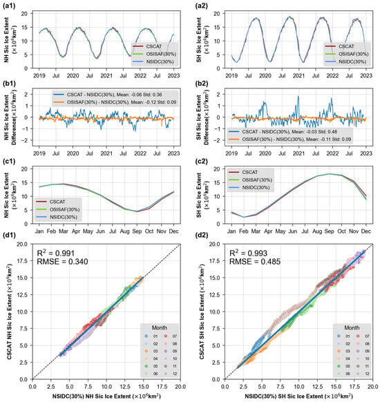
Figure 13.
Daily sea ice extent from 2019 to 2022 in the (a1) Northern Hemisphere and (a2) Southern Hemisphere for CSCAT, OSISAF (30% SIC), and NSIDC (30% SIC). Daily sea ice extent difference from 2019 to 2022 in the (b1) Northern Hemisphere and (b2) Southern Hemisphere for CSCAT vs. NSIDC and OSISAF vs. NSIDC. Monthly sea ice extent from 2019 to 2022 over the (c1) Northern Hemisphere and (c2) Southern Hemisphere for CSCAT, OSISAF (30% SIC), and NSIDC (30% SIC). Scatter plot of sea ice extent between CSCAT and NSIDC over the (d1) Northern Hemisphere and (d2) Southern Hemisphere. The pairs are colored by month, and the blue line represents a trend line fitted to the data.
To better present the results, we have graphically displayed the daily sea ice extent on a monthly basis. The visualization showed that sea ice extent from CSCAT matched NSIDC in January, February, May, June, July, and August. However, the results were slightly overestimated in March and April and slightly underestimated from September to December. In the Southern Hemisphere, the sea ice extent in February, August, and September corresponded closely, yet we observed an underestimation from March to July and an overestimation from November to January of the following year. These variations indicated that while the model performed well under specific conditions, such as during months with relatively stable sea ice conditions, its applicability under other conditions, particularly during seasonal transitions, was challenged. The observed underestimations or overestimations were likely associated with dynamic environmental factors that significantly impacted sea ice formation and melting during these transitional periods. This is in stark contrast to the discrepancies found between QuikSCAT and ASCAT compared to AMSR-E, particularly during sea ice melt months, as reported by Belmonte Rivas et al. [19]. It is noteworthy that active scatterometers and passive microwave radiometers showed significant differences during periods of rapid sea ice change. Furthermore, linear regression analysis of the CSCAT and NSIDC sea ice extent data yielded R-squared values of 0.991 and 0.993 with corresponding RMSE values of 0.340 and 0.485 million km2. These results confirm that our method for estimating sea ice extent provided consistent results over longer time periods compared to other accepted data sources.
4.2. Comparison with Sea Ice Concentration and Sea Ice Edge Datasets
ASCAT, SSMIS, and AMSR2 are the three other sources of sea ice cover data. ASCAT is a C-band HH-polarized scatterometer that provides sea ice detection similar to CSCAT. SSMIS and AMSR2 are the two dominant microwave radiometric instruments commonly used to determine sea ice concentration and provide more reliable sea ice distributions. To compare the spatial differences between the CSCAT sea ice edge and other sea ice cover products, we selected the sea ice edge from ASCAT and sea ice concentration from NSIDC. The comparison involved contrasting the CSCAT and ASCAT sea ice edges with the SSMIS sea ice concentration. This comparison employed a statistical method similar to a confusion matrix (Equation (6)). First, the NSIDC sea ice concentration was divided into three classes based on thresholds: less than 30% was open water (OW), 30–70% was open ice (OI), and more than 70% was close ice (CI). The CSCAT and ASCAT sea ice edge results also included these three types. Monthly mode statistics were calculated for each pixel compared to the NSIDC sea ice edge, resulting in the monthly average differences for sea ice edge between CSCAT, ASCAT, and NSIDC. The consistency of , and can be calculated using Equation (7).
For this study, we compared sea ice detection in the Northern Hemisphere on 10 January 2019 and in the Southern Hemisphere on 10 June 2019 from threedifferent sources: CSCAT, ASCAT, and NSIDC (Figure 14). The results of each data source were represented by a color-coded scale indicating the sea ice concentration and sea ice edge results. For NSIDC SIC, the scale ranges from dark red (0%, open water) to deep purple (100%, close ice). For sea ice edge products, the scale ranges from dark blue (open water) to light blue (open ice) to white (close ice). The comparison results indicate that the sea ice edge obtained by CSCAT was consistent with the sea ice acquired by ASCAT and NSIDC, but there were also some deviations. In the Northern Hemisphere, CSCAT detected open ice in the Greenland Sea, Baffin Bay, and Hudson Bay, while in the Southern Hemisphere, open ice was detected at the ice edge regions of the Ross Sea. Compared to ASCAT, this open ice tended to be less, which can also be observed in the sea ice distribution detected by Li et al. [21] using GMFs.
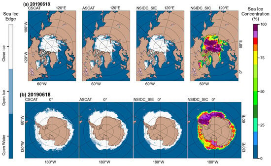
Figure 14.
Sea ice mapping in the (a) Northern Hemisphere on 18 June 2019 and (b) Southern Hemisphere on 18 June 2019 derived from CSCAT, ASCAT, NSIDC sea ice edge (SIE), and NSIDC sea ice concentration (SIC), respectively.
From the consistency time series for sea ice edge (Figure 15), it was observed that, in both the Southern and Northern Hemispheres, the consistency of close ice observed by CSCAT with that observed by NSIDC (0.903, 0.931) was slightly better than that of ASCAT (0.898, 0.922), while ASCAT (0.998, 0.997) showed slightly better performance for open water compared to CSCAT (0.988, 0.988). For open ice, CSCAT performed worse overall than ASCAT, although with slight differences in the different hemispheres. In the Northern Hemisphere, CSCAT showed lower consistency with NSIDC compared to ASCAT in most months. In the Southern Hemisphere, the differences between ASCAT and CSCAT in terms of open ice exhibited a seasonal symmetry: in the months when the consistency of ASCAT was poor (January to April), CSCAT performed well, and in the months when the consistency of CSCAT was poor (May to December), ASCAT performed well. This seasonal symmetry for the consistency of open ice in the Southern Hemisphere was also observed in Zhai et al. [23]. This suggested that CSCAT had a better ability to identify open ice compared to ASCAT from January to April. These differences were mainly due to the different frequencies of the two sensors. CSCAT operates in the Ku band, which has a shorter wavelength than the C-band ASCAT. The shorter wavelength is more sensitive to the rough surface of multiyear ice but has a weaker response to thin ice edges.
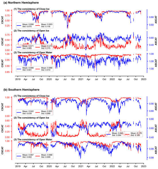
Figure 15.
Daily consistency compared to NSIDC for (1) close ice, (2) open ice, and (3) open water over the (a) Northern Hemisphere and (b) Southern Hemisphere from 1 January 2019 to 31 December 2022, respectively.
In the Northern Hemisphere, CSCAT showed lower consistency for open ice from January to April and lower consistency for close ice from May to August (Figure 15a (1),(2)). The spatial distribution of sea ice cover differences between CSCAT, ASCAT, and NSIDC in February and May revealed that the misclassification of sea ice by CSCAT in the Northern Hemisphere was mainly concentrated along the ice edges in the Barents Sea and the Greenland Sea, where close ice was incorrectly classified as open ice, which was less common in the spatial differences observed with ASCAT (Figure 16a,c). In August, CSCAT misclassified open ice as close ice, especially in the northern sea areas of Canada, while ASCAT showed less misclassification in these areas. In the Southern Hemisphere, CSCAT showed lower consistency for open ice from April to December but higher consistency from January to March. Misclassification still occurred at the ice edge, with open ice being mostly classified as close ice in August and November (Figure 16b,d). In March, mutual misclassification between close and open ice occurred at the sea ice edge of East Antarctica.
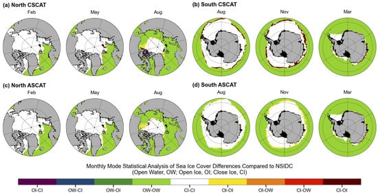
Figure 16.
Monthly mode statistics for CSCAT over the (a) Northern Hemisphere and (b) Southern Hemisphere and for ASCAT over the (c) Northern Hemisphere and (d) Southern Hemisphere, showing sea ice cover differences compared to NSIDC.
The comparison between CSCAT and ASCAT revealed that CSCAT had slightly better consistency with NSIDC for close ice in both hemispheres, while ASCAT performed better for open water. CSCAT generally underperformed compared to ASCAT for open ice, especially in the Northern Hemisphere. However, in the Southern Hemisphere, CSCAT outperformed ASCAT from January to April, whereas ASCAT performed better from May to December. Misclassifications were primarily observed along the ice edges in the Barents Sea and Greenland Sea, where CSCAT often misclassified close ice as open ice, unlike ASCAT. In August, CSCAT also misclassified open ice as close ice in central sea areas, while ASCAT’s misclassifications occurred mainly at the boundary between open and close ice. In the Southern Hemisphere, CSCAT showed lower consistency in detecting open ice from April to December but higher consistency from January to March, with misclassifications mostly occurring along the ice edges.
4.3. Comparison with High Resolution SAR Imagery
To confirm the regional detection of sea ice, a comparison with Sentinel-1 SAR data was performed. For the validation process, a section of the Northern Hemisphere on 19 June and 8 March 2019 and a section of the Southern Hemisphere on 19 June 2019 were selected and verified using the map data. During the process, we performed various data processing procedures using the SNAP 8.0.0 software, namely orbital corrections, radiometric calibrations, dB conversions, and latitude/longitude projections. We then created a geo-mosaic using ArcGIS 10.7 software, which allowed us to create SAR images covering many parts of the polar regions. In addition, we used ArcGIS software to extract the peripheral sea ice boundary from the sea ice results and overlay it on the corresponding SAR image.
Figure 17a depicts the expanse of open ice in the Greenland Sea as captured by the Sentinel-1 SAR imagery. The open ice appears as a lighter shade of gray in contrast to the deep gray of the seawater. The features observed were consistent with the sea ice boundaries extracted by CSCAT. Moreover, the Sentinel-1 SAR image dated 8 March 2019, facilitated the clear identification of sea ice and open water in Baffin Bay. This identification closely aligned with our extracted sea ice boundary positions, as illustrated in Figure 17b. Similar outcomes were demonstrated over two regions in the Southern Hemisphere above the Indian Ocean. The sea ice boundaries extracted by CSCAT showed superior performance in delineating sea ice from open waters (Figure 17c). Near the Antarctic Peninsula, CSCAT’s detection of sea ice boundaries differed from the SAR images and incorrectly marked some open water as sea ice. Despite this, CSCAT had accurately identified a distinct, isolated region of sea ice. Our detection results showed similarity in the shape and position of sea ice compared to Sentinel-1 SAR imagery while also capturing the variations and structural features at the sea ice edge.
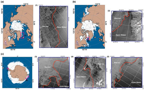
Figure 17.
Comparative analysis of sea ice detection and high-resolution synthetic aperture radar (SAR) images. Comparison between CSCAT-derived sea ice detection results and Sentinel-1 SAR images in the Northern Hemisphere taken on (a) 18 June 2019 and (b) 8 March 2019 and in the Southern Hemisphere on (c) 19 June 2019. The thick red line represents the CSCAT-derived sea ice detection results.
5. Conclusions
The aim of this study was to automatically extract feature information from CSCAT using PCA to retrieve sea ice data in the Northern and Southern Hemispheres and to use an ensemble machine learning algorithm to obtain reliable daily sea ice distributions from 2019 to 2022. PCA effectively extracted principal component features representing outer swath, zones, and close ice. We trained ensemble models based on Knn, Log, Dt, Gnb, and Rfc. Rfc/Knn exhibited high error rates in detecting open ice, often misclassifying it as close ice, particularly at the sea ice boundary. In contrast, Dt/Log/Gnb performed more effectively in identifying open ice at the sea ice boundary. By combining these models, we improved overall classification accuracy both for open ice and close ice. The sea ice edge detected by CSCAT was also independently validated against NSIDC’s sea ice concentration and ASCAT’s sea ice edge, showing high correlation in sea ice extent and temporal–spatial consistency as well as good alignment with SAR imagery at the sea ice–water boundary. The PCA extraction method significantly enhances the feature extraction capabilities of scatterometers with fan-beam and rotating-beam configurations. It complements traditional sea ice detection approaches and allows for the precise and reliable classification of sea ice and open water. Although CSCAT performed well in distinguishing between sea ice and open water, it was prone to confusion between different types of sea ice, with especially limited capability to identify open ice. In the Arctic, such misclassifications were most notable in the Greenland Sea in February and May and in parts of the central region in August; in the Antarctic, they were primarily observed across the entire Antarctic sea ice–water boundary in August and November and along the Antarctic coastline and sea water boundary in May. Open ice is typically associated with the marginal ice zone (MIZ), which is more important than the central region (close ice) for shipping route development, fishery resources, ecosystems, and climate responses. So, good performance on open ice is more important. Future work should focus on further optimizing the algorithm to improve open ice recognition and extending its application to other radar systems, incorporating additional data from ship-based observations, optical imagery, and SAR to enhance detection performance.
Author Contributions
Y.L. (Yanping Luo): investigation, conceptualization, methodology, data curation, writing—original draft, writing—review and editing. Y.L. (Yang Liu): conceptualization, formal analysis, writing—review and editing. C.H.: methodology, data curation. F.H.: methodology, data curation. All authors contributed to the manuscript and approved the submitted version. All authors have read and agreed to the published version of the manuscript.
Funding
This work was supported by the research program “Impact and Response of Antarctic Seas to Climate Change, IRASCC2020-2022” (Grant No. IRASCC 01-02-05C) from the Chinese Arctic and Antarctic Administration (CAA), Ministry of Natural Resources of the People’s Republic of China.
Data Availability Statement
The data underlying this article will be shared upon reasonable request to the corresponding authors.
Conflicts of Interest
The authors declare no conflicts of interest.
References
- Turner, J.; Orr, A.; Gudmundsson, G.H.; Jenkins, A.; Bingham, R.G.; Hillenbrand, C.-D.; Bracegirdle, T.J. Atmosphere-ocean-ice interactions in the Amundsen Sea Embayment, West Antarctica. Rev. Geophys. 2017, 55, 235–276. [Google Scholar] [CrossRef]
- Boers, N. Observation-based early-warning signals for a collapse of the Atlantic Meridional Overturning Circulation. Nat. Clim. Chang. 2021, 11, 680–688. [Google Scholar] [CrossRef]
- Lin, Y.; Moreno, C.; Marchetti, A.; Ducklow, H.; Schofield, O.; Delage, E.; Meredith, M.; Li, Z.; Eveillard, D.; Chaffron, S.; et al. Decline in plankton diversity and carbon flux with reduced sea ice extent along the Western Antarctic Peninsula. Nat. Commun. 2021, 12, 4948. [Google Scholar] [CrossRef] [PubMed]
- Gui, D.; Pang, X.; Lei, R.; Zhao, X.; Wang, J. Changes in sea ice kinematics in the Arctic outflow region and their associations with Arctic Northeast Passage accessibility. Acta Oceanol. Sin. 2019, 38, 101–110. [Google Scholar] [CrossRef]
- Comiso, J.C.; Meier, W.N.; Gersten, R. Variability and trends in the Arctic Sea ice cover: Results from different techniques. J. Geophys. Res. Ocean. 2017, 122, 6883–6900. [Google Scholar] [CrossRef]
- Comiso, J.C.; Gersten, R.A.; Stock, L.V.; Turner, J.; Perez, G.J.; Cho, K. Positive Trend in the Antarctic Sea Ice Cover and Associated Changes in Surface Temperature. J. Clim. 2017, 30, 2251–2267. [Google Scholar] [CrossRef]
- Turner, J.; Hosking, J.S.; Phillips, T.; Marshall, G.J. Temporal and spatial evolution of the Antarctic sea ice prior to the September 2012 record maximum extent. Geophys. Res. Lett. 2013, 40, 5894–5898. [Google Scholar] [CrossRef]
- Lieser, J.; Massom, R.; Reid, P.; Scambos, T.; Stammerjohn, S. The record 2013 Southern Hemisphere sea-ice extent maximum. Ann. Glaciol. 2015, 56, 99–106. [Google Scholar] [CrossRef]
- Turner, J.; Phillips, T.; Marshall, G.J.; Hosking, J.S.; Pope, J.O.; Bracegirdle, T.J.; Deb, P. Unprecedented springtime retreat of Antarctic sea ice in 2016. Geophys. Res. Lett. 2017, 44, 6868–6875. [Google Scholar] [CrossRef]
- Cohen, J.; Screen, J.A.; Furtado, J.C.; Barlow, M.; Whittleston, D.; Coumou, D.; Francis, J.; Dethloff, K.; Entekhabi, D.; Overland, J.; et al. Recent Arctic amplification and extreme mid-latitude weather. Nat. Geosci. 2014, 7, 627–637. [Google Scholar] [CrossRef]
- Sandven, S.; Johannessen, O.M. The use of microwave remote sensing for sea ice studies in the Barents Sea. ISPRS J. Photogramm. Remote Sens. 1993, 48, 2–18. [Google Scholar] [CrossRef]
- Zhang, P.; Hu, X.; Lu, Q.; Zhu, A.; Lin, M.; Sun, L.; Chen, L.; Xu, N. FY-3E: The First Operational Meteorological Satellite Mission in an Early Morning Orbit. Adv. Atmos. Sci. 2022, 39, 1–8. [Google Scholar] [CrossRef]
- Remund, Q.P.; Long, D.G. Sea ice extent mapping using Ku band scatterometer data. J. Geophys. Res. Ocean. 1999, 104, 11515–11527. [Google Scholar] [CrossRef]
- Remund, Q.P.; Long, D.G. A Decade of QuikSCAT Scatterometer Sea Ice Extent Data. IEEE Trans. Geosci. Remote Sens. 2014, 52, 4281–4290. [Google Scholar] [CrossRef]
- Abreu, R.D.; Wilson, K.; Arkett, M.; Langlois, D. Evaluating the use of QuikSCAT data for operational sea ice monitoring. In Proceedings of the IEEE International Geoscience and Remote Sensing Symposium, Toronto, ON, Canada, 24–28 June 2002; Volume 3035, pp. 3032–3033. [Google Scholar]
- Li, M.; Zhao, C.; Zhao, Y.; Wang, Z.; Shi, L. Polar Sea Ice Monitoring Using HY-2A Scatterometer Measurements. Remote Sens. 2016, 8, 688. [Google Scholar] [CrossRef]
- de Haan, S.; Stoffelen, A. Ice Discrimination Using ERS Scatterometer. 2001. Available online: https://www.knmi.nl/research/publications/ice-discrimination-using-ers-scatterometer (accessed on 23 August 2024).
- Verspeek, J.A. Sea Ice Classification Using Bayesian Statistics; KNMI, 2006. Available online: https://www.knmi.nl/research/publications/sea-ice-classification-using-bayesian-statistics (accessed on 23 August 2024).
- Belmonte Rivas, M.; Verspeek, J.; Verhoef, A.; Stoffelen, A. Bayesian Sea Ice Detection With the Advanced Scatterometer ASCAT. IEEE Trans. Geosci. Remote Sens. 2012, 50, 2649–2657. [Google Scholar] [CrossRef]
- Belmonte Rivas, M.; Stoffelen, A. New Bayesian Algorithm for Sea Ice Detection With QuikSCAT. IEEE Trans. Geosci. Remote Sens. 2011, 49, 1894–1901. [Google Scholar] [CrossRef]
- Li, Z.; Verhoef, A.; Stoffelen, A. Bayesian Sea Ice Detection Algorithm for CFOSAT. Remote Sens. 2022, 14, 3569. [Google Scholar] [CrossRef]
- Hersbach, H.; Stoffelen, A.; de Haan, S. An improved C-band scatterometer ocean geophysical model function: CMOD5. J. Geophys. Res. Ocean. 2007, 112, C03006. [Google Scholar] [CrossRef]
- Zhai, X.; Wang, Z.; Zheng, Z.; Xu, R.; Dou, F.; Xu, N.; Zhang, X. Sea Ice Monitoring with CFOSAT Scatterometer Measurements Using Random Forest Classifier. Remote Sens. 2021, 13, 4686. [Google Scholar] [CrossRef]
- Liu, L.; Dong, X.; Lin, W.; Lang, S.; Wang, L. Polar Sea Ice Detection with the CFOSAT Scatterometer. In Proceedings of the 2021 IEEE International Geoscience and Remote Sensing Symposium IGARSS, Brussels, Belgium, 11–16 July 2021; pp. 5645–5648. [Google Scholar] [CrossRef]
- Xu, R.; Zhao, C.; Zhai, X.; Chen, G. Arctic Sea Ice Type Classification by Combining CFOSCAT and AMSR-2 Data. Earth Space Sci. 2022, 9, e2021EA002052. [Google Scholar] [CrossRef]
- Hotelling, H. Analysis of a complex of statistical variables into principal components. J. Educ. Psychol. 1933, 24, 498–520. [Google Scholar] [CrossRef]
- Zabalza, J.; Ren, J.; Yang, M.; Zhang, Y.; Wang, J.; Marshall, S.; Han, J. Novel Folded-PCA for improved feature extraction and data reduction with hyperspectral imaging and SAR in remote sensing. ISPRS J. Photogramm. Remote Sens. 2014, 93, 112–122. [Google Scholar] [CrossRef]
- Singh, R.K.; Singh, K.N.; Maisnam, M.; P., J.; Maity, S. Antarctic Sea Ice Extent from ISRO’s SCATSAT-1 Using PCA and An Unsupervised Classification. Proceedings 2018, 2, 340. [Google Scholar] [CrossRef]
- Long, D.G. Polar Applications of Spaceborne Scatterometers. IEEE J. Sel. Top. Appl. Earth Obs. Remote Sens. 2017, 10, 2307–2320. [Google Scholar] [CrossRef]
- Yueh, S.H.; Kwok, R.; Lou, S.H.; Tsai, W.Y. Sea ice identification using dual-polarized Ku-band scatterometer data. IEEE Trans. Geosci. Remote Sens. 1997, 35, 560–569. [Google Scholar] [CrossRef]
- Breivik, L.A.; Eastwood, S.; Lavergne, T. Use of C-Band Scatterometer for Sea Ice Edge Identification. IEEE Trans. Geosci. Remote Sens. 2012, 50, 2669–2677. [Google Scholar] [CrossRef]
- Lindell, D.; Long, D. Multiyear Arctic Ice Classification Using ASCAT and SSMIS. Remote Sens. 2016, 8, 294. [Google Scholar] [CrossRef]
- Aaboe, S.; Down, E.J.; Eastwood, S. EUMETSAT Ocean and Sea Ice Satellite Application Facility, Global Seaice Edge Near-Real-Time Product-Multimission (2020), OSI-402-d, (Data Extracted from OSI SAF FTP Server/EUMETSAT Data Center: Accessed 10-01-2023. 2020. Available online: https://osi-saf.eumetsat.int/products/osi-402-d (accessed on 23 August 2024).
- Hill, J.C.; Long, D.G. Extension of the QuikSCAT Sea Ice Extent Data Set with OSCAT Data. IEEE Geosci. Remote Sens. Lett. 2017, 14, 92–96. [Google Scholar] [CrossRef]
- Xu, R.; Zhao, C.; Zhai, X.; Zhao, K.; Shen, J.; Chen, G. Polar Sea Ice Identification and Classification Based on HY-2A/SCAT Data. J. Ocean Univ. China 2022, 21, 331–346. [Google Scholar] [CrossRef]
- Zou, J.; Zeng, T.; Guo, M.; Cui, S. The study on an Antarctic sea ice identification algorithm of the HY-2A microwave scatterometer data. Acta Oceanol. Sin. 2016, 35, 74–79. [Google Scholar] [CrossRef]
- Liu, L.; Zhai, H.; Dong, X.; Zhao, F. SEA ICE Extent Retrieval with Ku-Band Rotating Fan Beam Scatterometer Data. In Proceedings of the IGARSS 2022-2022 IEEE International Geoscience and Remote Sensing Symposium, Kuala Lumpur, Malaysia, 17–22 July 2022; pp. 3810–3813. [Google Scholar] [CrossRef]
- Xu, C.; Wang, Z.; Zhai, X.; Lin, W.; He, Y. SVM-Based Sea Ice Extent Retrieval Using Multisource Scatterometer Measurements. Remote Sens. 2023, 15, 1630. [Google Scholar] [CrossRef]
- Zhai, X.; Tian, S.; Ye, Y.; Cao, G.; Chen, L.; Xu, N.; Zheng, Z. First Results of Antarctic Sea Ice Classification Using Spaceborne Dual-Frequency Scatterometer FY-3E WindRAD. IEEE Geosci. Remote Sens. Lett. 2024, 21, 2000105. [Google Scholar] [CrossRef]
- Li, Z.; Stoffelen, A.; Verhoef, A.; Verspeek, J. Numerical Weather Prediction Ocean Calibration for the Chinese-French Oceanography Satellite Wind Scatterometer and Wind Retrieval Evaluation. Earth Space Sci. 2021, 8, e2020EA001606. [Google Scholar] [CrossRef]
- Li, Z.; Stoffelen, A.; Verhoef, A.; Verspeek, J. NWP Ocean Calibration for the CFOSAT Wind Scatterometer. In Proceedings of the 2021 IEEE International Geoscience and Remote Sensing Symposium IGARSS, Brussels, Belgium, 11–16 July 2021; pp. 443–446. [Google Scholar] [CrossRef]
- Zhang, K.; Dong, X.; Zhu, D.; Yun, R.; Wang, B.; Yu, M. An Improved Method of Noise Subtraction for the CFOSAT Scatterometer. IEEE J. Sel. Top. Appl. Earth Obs. Remote Sens. 2021, 14, 7506–7515. [Google Scholar] [CrossRef]
- Ivanova, N.; Pedersen, L.T.; Tonboe, R.T.; Kern, S.; Heygster, G.; Lavergne, T.; Sørensen, A.; Saldo, R.; Dybkjær, G.; Brucker, L.; et al. Inter-comparison and evaluation of sea ice algorithms: Towards further identification of challenges and optimal approach using passive microwave observations. Cryosphere 2015, 9, 1797–1817. [Google Scholar] [CrossRef]
- Kern, S.; Lavergne, T.; Notz, D.; Pedersen, L.T.; Tonboe, R.T.; Saldo, R.; Sørensen, A.M. Satellite passive microwave sea-ice concentration data set intercomparison: Closed ice and ship-based observations. Cryosphere 2019, 13, 3261–3307. [Google Scholar] [CrossRef]
- Comiso, J.C. Characteristics of Arctic winter sea ice from satellite multispectral microwave observations. J. Geophys. Res. Ocean. 1986, 91, 975–994. [Google Scholar] [CrossRef]
- Smith, D.M. Extraction of winter total sea-ice concentration in the Greenland and Barents Seas from SSM/I data. Int. J. Remote Sens. 1996, 17, 2625–2646. [Google Scholar] [CrossRef]
- Lavergne, T.; Sørensen, A.M.; Kern, S.; Tonboe, R.; Notz, D.; Aaboe, S.; Bell, L.; Dybkjær, G.; Eastwood, S.; Gabarro, C.; et al. Version 2 of the EUMETSAT OSI SAF and ESA CCI sea-ice concentration climate data records. Cryosphere 2019, 13, 49–78. [Google Scholar] [CrossRef]
- Cavalieri, D.J.; Parkinson, C.; Gloersen, P.; Zwally, H.J. Sea Ice Concentrations from Nimbus-7 SMMR and DMSP SSM/I-SSMIS Passive Microwave Data. 1996. Available online: https://nsidc.org/data/nsidc-0051/versions/1 (accessed on 21 January 2023).
- Cavalieri, D.J.; Gloersen, P.; Campbell, W.J. Determination of sea ice parameters with the Nimbus 7 SMMR. J. Geophys. Res. Atmos. 1984, 89, 5355–5369. [Google Scholar] [CrossRef]
- Dabboor, M.; Shokr, M. A new Likelihood Ratio for supervised classification of fully polarimetric SAR data: An application for sea ice type mapping. ISPRS J. Photogramm. Remote Sens. 2013, 84, 1–11. [Google Scholar] [CrossRef]
- Torres, R.; Snoeij, P.; Geudtner, D.; Bibby, D.; Davidson, M.; Attema, E.; Potin, P.; Rommen, B.; Floury, N.; Brown, M.; et al. GMES Sentinel-1 mission. Remote Sens. Environ. 2012, 120, 9–24. [Google Scholar] [CrossRef]
- Stewart, J.S.; Meier, W.N.; Scott, D.J. Polar Stereographic Ancillary Grid Information, Version 1; National Snow and Ice Data Center: Boulder, CO, USA, 2022. [Google Scholar] [CrossRef]
- Meier, W.N.; Stroeve, J.; Fetterer, F.; Wilcox, H. Polar Stereographic Valid Ice Masks Derived from National Ice Center Monthly Sea Ice Climatologies, Version 1; National Snow and Ice Data Center: Boulder, CO, USA, 2015. [Google Scholar] [CrossRef]
- Halko, N.; Martinsson, P.-G.; Tropp, J.A. Finding structure with randomness: Stochastic algorithms for constructing approximate matrix decompositions. arXiv 2009, arXiv:0909.4061. [Google Scholar] [CrossRef]
- Sandven, S.; Spreen, G.; Heygster, G.; Girard-Ardhuin, F.; Farrell, S.L.; Dierking, W.; Allard, R.A. Sea Ice Remote Sensing—Recent Developments in Methods and Climate Data Sets. Surv. Geophys. 2023, 44, 1653–1689. [Google Scholar] [CrossRef]
- Hao, H.; Su, J.; Shi, Q.; Li, L. Arctic sea ice concentration retrieval using the DT-ASI algorithm based on FY-3B/MWRI data. Acta Oceanol. Sin. 2021, 40, 176–188. [Google Scholar] [CrossRef]
- Liu, J.; Liu, S.; Lin, W.; Lang, S.; He, Y. Sea ice identification based on CFOSAT scatterometer. Haiyang Xuebao 2023, 45, 134–140. [Google Scholar] [CrossRef]
- CAFF. Boundary for Conservation of Arctic Flora and Fauna (CAFF) Working Group of the Arctic Council. 2017. Available online: http://geo.abds.is/geonetwork/srv/eng/catalog.search#/metadata/2ad7a7cb-2ad7-4517-a26e-7878ef134239 (accessed on 1 December 2023).
- Fetterer, F.; Fetterer, F.; Knowles, K.; Meier, W.N.; Savoie, M.; Windnagel, A.K. Sea Ice Index, Version 3 [Data Set]; National Snow and Ice Data Center: Boulder, CO, USA, 2017; Available online: https://doi.org/10.7265/N5K072F8 (accessed on 10 January 2023).
- Kern, S.; Lavergne, T.; Notz, D.; Pedersen, L.T.; Tonboe, R. Satellite passive microwave sea-ice concentration data set inter-comparison for Arctic summer conditions. Cryosphere 2020, 14, 2469–2493. [Google Scholar] [CrossRef]
Disclaimer/Publisher’s Note: The statements, opinions and data contained in all publications are solely those of the individual author(s) and contributor(s) and not of MDPI and/or the editor(s). MDPI and/or the editor(s) disclaim responsibility for any injury to people or property resulting from any ideas, methods, instructions or products referred to in the content. |
© 2024 by the authors. Licensee MDPI, Basel, Switzerland. This article is an open access article distributed under the terms and conditions of the Creative Commons Attribution (CC BY) license (https://creativecommons.org/licenses/by/4.0/).