Abstract
Estimating tropical cyclone (TC) intensity is crucial for disaster reduction and risk management. This study aims to estimate TC intensity using machine learning (ML) models. We utilized eight ML models to predict TC intensity, incorporating factors such as TC location, central pressure, distance to land, landfall in the next six hours, storm speed, storm direction, date, and number from the International Best Track Archive for Climate Stewardship Version 4 (IBTrACS V4). The dataset was divided into four sub-datasets based on the El Niño–Southern Oscillation (ENSO) phases (Neutral, El Niño, and La Niña). Our results highlight that central pressure has the greatest effect on TC intensity estimation, with a maximum root mean square error (RMSE) of 1.289 knots (equivalent to 0.663 m/s). Cubist and Random Forest (RF) models consistently outperformed others, with Cubist showing superior performance in both training and testing datasets. The highest bias was observed in SVM models. Temporal analysis revealed the highest mean error in January and November, and the lowest in February. Errors during the Warm phase of ENSO were notably higher, especially in the South China Sea. Central pressure was identified as the most influential factor for TC intensity estimation, with further exploration of environmental features recommended for model robustness.
1. Introduction
Tropical cyclones (TCs) are among the most devastating natural phenomena, capable of causing immense destruction and loss of life upon making landfall in coastal areas [1]. Their frequency and intensity are closely related to climate change and extreme weather patterns, making their study increasingly critical in the context of a warming planet [2]. Accurate estimation of TC intensity is essential for predicting potential impacts and implementing effective mitigation strategies.
Numerous theoretical models and techniques have been developed to estimate TC intensity, each with its strengths and limitations. The Dvorak technique is one of the most widely used methods, leveraging satellite imagery to assess storm intensity [3,4]. The Dvorak technique has been enhanced with the objective Dvorak technique (ODT) and advanced ODT (AODT) to better assess the inner core structure and evolution of TCs [5,6]. Additionally, based on that method, the Liou–Liu formula was introduced to investigate the interaction, especially intensity interaction, between two TCs or TCs and TDs [7,8]. Other methods, such as an image processing approach using feature vector analysis, have also been proposed for TC intensity detection [9]. These methods typically rely on satellite imagery and cloud characteristics to estimate TC intensity.
Numerical weather prediction models offer dynamic simulations based on atmospheric data, providing detailed forecasts. The primary source of uncertainty in predicting storm intensity lies in the variability of the forecasted environmental wind shear [10]. Lee et al. [11] used a probabilistic multiple linear regression model to relate TC intensity to the local large-scale environment, with promising results. Bhattacharya et al. [12] developed an empirical relationship between model mean sea level pressure and observed intensity, which improved intensity prediction. Davis [13] highlighted the importance of model resolution in accurately representing TC intensity, particularly for category 4 and 5 storms.
Recent progress in machine learning (ML) and deep learning (DL) have introduced new approaches, enabling more sophisticated and accurate predictions by analyzing large datasets and recognizing complex patterns. While ML and DL techniques are still being actively researched and developed for TC forecasting, recent studies have shown promising results in their application, whether through employing pure data-driven models or enhancing mathematical models. This includes TC eye recognition based on intensity prediction, image contour extraction, and various ML techniques [14,15,16]. Recent studies have shown promising results in the use of ML for estimation of TC intensity. Biswas et al. [17] achieved an 88% accuracy in cyclone grade estimation and a root mean square error (RMSE) of 2.3 in maximum sustained surface wind speed estimation over the North Indian Ocean. Olander et al. [18] developed an enhanced advanced Dvorak technique (AiDT) model, which demonstrated a 30% improvement in MSWS estimation over the traditional advanced Dvorak technique. Zhang et al. [19] proposed a relevance vector machine model for TC intensity estimation using infrared satellite image data, showing potential for improved accuracy. Tan et al. [20] used Himawari-8 satellite cloud products and DL to achieve a relatively low RMSE of 4.06 m/s and a mean absolute error (MAE) of 3.23 m/s in TC intensity estimation. These studies collectively highlight the potential of ML in improving the accuracy of TC intensity estimation. Jiang et al. [21] proposed a deep multisource attention network (DMANet) for TC intensity estimation, achieving a significant reduction in RMSE.
This work explores the probable application of ML methods to TC intensity estimation over the Western North Pacific (WNP). Four groups of ML methods were considered: (a) linear, (b) tree-based, (c) instance-based, and (d) boosting. The main objective is to improve TC intensity prediction by applying eight different regression-based ML models to a comprehensive dataset of 1017 typhoons from the International Best Track Archive for Climate Stewardship (IbTRACS). Recognizing the influence of the El Niño–Southern Oscillation (ENSO) on TC activity, the analysis considers four distinct phases of ENSO, resulting in a total of 32 model instances being evaluated. To compare the performance of these ML methods, four statistical indices were used: coefficient of determination (R2), Nash–Sutcliffe Efficiency (NSE), MAE, and RMSE. By extracting critical features from the typhoon data and applying these models, the study seeks to provide a more accurate and nuanced understanding of TC intensity across different ENSO phases. This approach not only aims to enhance predictive accuracy, but also to offer insights into the complex interactions between TCs and climate variability.
2. Materials and Methods
2.1. Data and Preprocessing Data
2.1.1. TC Best-Track Dataset
The data for this research were collected from the International Best Track Archive for Climate Stewardship Version 4 (IBTrACS V4) dataset. This dataset was created in collaboration with all of the World Meteorological Organization’s Regional Specialized Meteorological Centers (RSMCs) and provides a comprehensive collection of information about TCs across the globe [22]. The scope of this research pertains solely to mature typhoon phases, omitting instances where wind speeds are less than 35 knots. The 6-hourly center estimates from IBTrACS for typhoons from 1979 to 2020 in the WNP are shown in Figure 1. For the NWP Ocean zone, the IBTrACS dataset contains 1017 typhoon data collected by the RSMC–Tokyo center of the Japan Meteorological Agency (JMA) from 1979 to 2020. The dataset had mostly 6-hourly data points, along with a few 3-hourly and 1-hourly data points. To smooth the whole dataset for statistical purposes, all 3-hourly and 1-hourly data points were removed. Factors under scrutiny encompass typhoon identity, number, location (including longitude and latitude), maximum wind speed, minimum central pressure, storm direction, storm speed, distance to land, landfall in the next 6 h, and date within the WNP. The 6-hourly interval between track points in the IBTrACS dataset supports its use as input for ML models, as IBTrACS was created for this purpose. However, it is important to note that while this uniform interval aids in the structured input for models, it does not guarantee perfectly accurate tracking or precision, as IBTrACS may involve interpolation and subjectivity in forecast centers.
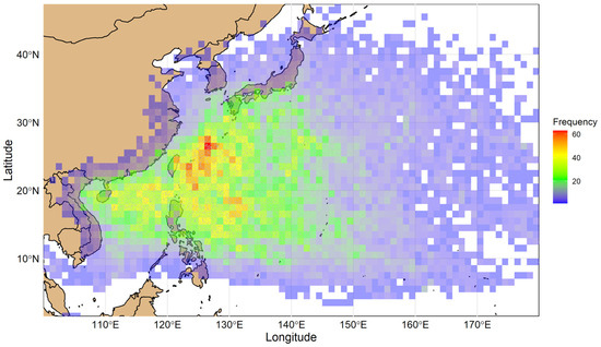
Figure 1.
Two-dimensional histogram showing the frequency (count) of 6-hourly center estimates from the IBTrACS dataset for TCs in the WNP from 1979 to 2020. The histogram is overlaid with actual track points (grey dots), with each bin representing a 1° × 1° degree resolution.
2.1.2. Study Area
The WNP region, including countries like Vietnam, Japan, China, the Philippines, and Taiwan, is particularly notable for its frequent and intense typhoons. These powerful typhoons significantly impact the region, causing extensive damage and necessitating robust disaster preparedness and response strategies. Typhoons primarily form between May and November, with their intensity and frequency influenced by climatic factors.
2.1.3. Multivariate ENSO Index Version 2 (MEI V2)
ENSO is a recurring climate phenomenon occurring approximately every 2 to 7 years, characterized by changes in sea surface temperature (El Niño and La Niña) and atmospheric air pressure (Southern Oscillation) across the equatorial Pacific Ocean. These oceanic and atmospheric dynamics interact in complex ways that influence typhoons differently during each ENSO phase. The bi-monthly MEI V2 was utilized to investigate ENSO’s impact on typhoons. Data spanning from 1979 to 2020 were extracted from https://www.psl.noaa.gov/enso/mei/ (accessed on 1 January 2023). ENSO phases were categorized as Neutral (values near ±0.5), El Niño (values > +0.5), and La Niña (values < −0.5).
2.2. Methods
The research workflow consists of three main stages: data collection, model application, and model evaluation and comparison (Figure 2). Initially, typhoon data from the IBTrACS V4 and MEI V2 datasets were compiled into a standardized format, ensuring inclusion of both target and predictive variables. Only typhoon tracks within the WNP region were retained. Next, the Boruta algorithm was employed to identify features that significantly contribute to intensity estimation [23]. Subsequently, these selected factors were incorporated into the models. The dataset was then randomly split into training and testing subsets. The training data were used to optimize hyperparameters and develop predictive models using ML methods.
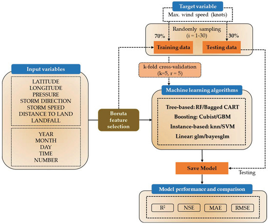
Figure 2.
Schematic flowchart of the current study.
The 12 predictors utilized in this study are latitude, longitude, pressure, storm direction, storm speed, distance to land, landfall, year, month, day, time, and number. This list is also depicted in Figure 2. The time feature was eliminated by Boruta feature selection. Therefore, we have 11 predictors as inputs to ML models. The dataset was partitioned into two sets using a 70/30 split, a common ratio employed in many studies. Table 1 summarizes the distribution of training and testing data across different phases of the ENSO. It shows the number of data points used for training and testing models under Neutral phase, El Niño (or Warm phase), and La Niña (or Cold phase) conditions, with a total of 24,485 data points allocated for analysis. The entire process was iterated thirty times to ensure model stability and facilitate comparisons between models. The training data underwent modeling with k-fold cross-validation, where the number of folds (k) was set to 5 and the process was repeated 5 times (r).

Table 1.
Amount of training and testing data in models.
The target variable represents the maximum wind speed of the typhoon at each estimated center point, which indicates the intensity of the TC. The latitude and longitude denote the location of the TC’s center at the time when it reaches its maximum intensity. TCs predominantly forms between 10°N and 30°N from the equator. Minimum central pressure refers to the lowest atmospheric pressure estimated at the center, or eye, of a TC. Storm direction refers to the path or trajectory along which the TC is moving. Storm speed indicates how quickly the TC is moving along its path. Distance to land is the current separation between the TC’s center and the nearest coastline or landmass. Landfall refers to the prediction of whether the TC is likely to cross over a coastline within the next six hours. This event marks where the TC’s center intersects the coastline. Year, month, day, and time are variables used to denote specific points in time within the IBTrACS dataset. The “number” typically serves as a unique identifier for each TC or storm system within a given basin, facilitating the tracking of their characteristics, trajectory, and impacts over time, though it may not be unique across all basins.
2.2.1. ML Models and Hyperparameters
This section describes the models and their hyperparameters used in the study. We selected eight distinct ML models from four categories: tree-based models, boosting models, instance-based models, and linear models. This selection provided a comprehensive overview of various ML approaches and their performance in estimating typhoon intensity. The models were implemented using R software 4.1.2, with detailed information provided in Table A1.
- Tree-based models
- Random Forest (RF): Implemented using the randomForest package in R (rf function), Random Forest consists of 2000 decision trees. Each tree is constructed by randomly selecting 5 variables at each split, providing robustness against overfitting and effective handling of complex data relationships [24].
- Bagged Classification and Regression Trees (CART): Utilized via the e1071 package (treebag function) without specific hyperparameter tuning. Bagged CART aggregates multiple decision trees to improve predictive accuracy and stability [25].
- Boosting models
- Gradient Boosting Machine (GBM): Developed with the gbm package (gbm function), GBM employs an ensemble of 100 trees. Each tree is sequentially built to correct errors of the previous one, with an interaction depth of 1, shrinkage of 0.1 to prevent overfitting, and requiring at least 10 observations per node for robust model construction [26,27].
- Cubist: Implemented using the cubist package (cubist function), Cubist utilizes 100 committees and employs 5 nearest neighbors for regression predictions. It combines rule-based models with model averaging techniques, effectively capturing nonlinear relationships in data [28].
- Instanced models
- K-Nearest Neighbors (kNN): Utilized via the caret package (knn function), kNN is employed with k set to 6 for classification tasks. It predicts based on the majority class among its nearest neighbors, making it suitable for clustered data points and non-parametric modeling [29].
- Support Vector Machine (SVM): Developed using the LiblineaR package (svmLinear3 function), SVM constructs hyperplanes in high-dimensional space. It is configured with a cost parameter of 1 and uses L2 loss (mean square error) for optimal fitting, offering robust performance in classification and regression tasks [30].
- Linear models
- Generalized linear models (GLMs): Implemented with the caret package (glm function), GLMs are versatile in modeling various types of linear relationships. They are used here without additional hyperparameter tuning, leveraging simplicity and interpretability for straightforward model implementation [31].
- Bayesian GLM: Developed using the arm package (bayesglm function), Bayesian GLM incorporates Bayesian inference for uncertainty quantification in predictions. It offers insights into parameter uncertainty and posterior distribution, enhancing the interpretability of model results [32].
2.2.2. Model Performance
To assess the performance of the ML models, four statistical indices were employed as assessment metrics: (1) coefficient of determination (R2), (2) root mean square error (RMSE), (3) mean absolute error (MAE), and (4) Nash–Sutcliffe Efficiency (NSE).
R2 measures the proportion of the variance in the dependent variable (e.g., maximum wind speed) that is predictable from the independent variables (model predictions). A higher R2 indicates a better fit of the model to the data, with values closer to 1 indicating stronger predictive power.
RMSE quantifies the average magnitude of the errors between estimated values and observed values. It offers a measure of the model’s accuracy, where lower RMSE values indicate better model performance in minimizing prediction errors.
MAE measures the average magnitude of the errors between estimated values and observed values, without considering the direction of errors. It delivers a straightforward assessment of forecast accuracy, with lower MAE values indicating better model performance in terms of absolute prediction error.
Nash–Sutcliffe Efficiency (NSE) assesses the predictive performance of hydrological models by comparing the simulated values to observed values. It ranges from negative infinity to 1, where 1 indicates perfect predictions, values closer to 0 indicate predictions are no better than the mean of the observed data, and negative values indicate predictions are worse than using the mean.
2.2.3. Important Factor Analysis
Permutation methods for defining variable importance are used to assess each predictor’s contribution in a model by measuring the impact on performance when a variable’s values are randomly shuffled. This technique begins by establishing a baseline performance metric with the original dataset. Then, the values of one variable are permuted, and the model’s performance is re-evaluated; a significant drop in performance indicates high importance, while a minor change suggests low importance. This method is versatile and model-agnostic, offering a straightforward way to understand and rank the importance of variables [33,34].
After obtaining these scores, they are ranked in order from most to least important, from 1 to 10. The final results are averaged across the two types of models that yield the best performance, incorporating four phases of ENSO models and 30 runs.
3. Results
In this part, we present a comparison of 32 instances of models, highlighting the two best-performing models based on statistical performance. Subsequent sections will detail the spatial distribution and monthly errors of these models. Finally, we analyze the important factors contributing to the performance of these top models.
3.1. Comparison of 32 Model Instances for Intensity Estimate
This section examines the performance of 32 model instances for estimating intensity, focusing on metrics such as NSE and RMSE. These metrics are derived from a comprehensive analysis involving 30 runs per model, resulting in a total of 120 data points across Figure 3a,b. Figure 3c,d provide a detailed summary of the results from the NSE and RMSE analyses, respectively, categorized by datasets (All Centers, Cold, Warm, and Neutral phases).
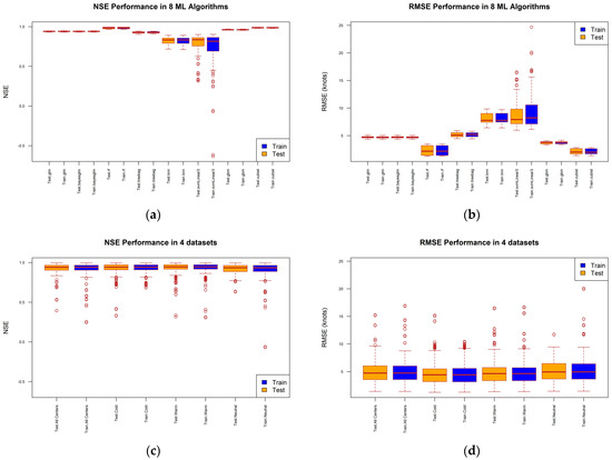
Figure 3.
Performance comparison of average models: (a,b) 8 types of models and (c,d) 4 datasets.
Among the models evaluated, Cubist consistently shows the lowest RMSE values across all datasets, ranging from 1.42 ± 0.023 (Cold phase in training) to 2.732 ± 0.057 (Neutral phase in testing). Following closely, RF demonstrates the second-lowest RMSE values, varying from 1.289 ± 0.009 (Cold phase in training) to 3.395 ± 0.072 (Neutral phase in testing). GBM also performs well, with RMSE values spanning from 3.381 ± 0.022 (Cold phase in training) to 4.024 ± 0.052 (Neutral phase in testing). Conversely, kNN and SVM with a Linear Kernel exhibit relatively higher RMSE values across datasets, with kNN ranging from 7.316 ± 0.05 (Warm phase in training) to 9.737 ± 3.975 (Neutral phase in testing), and SVM varying from 8.143 ± 2.202 (Cold phase in testing) to 9.737 ± 3.975 (Neutral phase in testing). The GLM and Bayesian GLM models demonstrate consistent RMSE values across different datasets, maintaining values like 4.651 ± 0.023 (in training) and 4.653 ± 0.055 (in testing) for both GLM and Bayesian GLM in the Warm phase dataset as an example (as shown in Table 2).

Table 2.
Performance indices of 32 model instances for training and testing data.
Cubist demonstrates the highest NSE values across various datasets, ranging from 0.98 ± 0.001 (Neutral phase in testing) to 0.994 ± 0 (Cold phase in training). RF follows closely with NSE values spanning from 0.969 ± 0.001 (Neutral phase in testing) to 0.995 ± 0 (All Centers, Cold, and Warm phases in training). GBM also performs well, with NSE values ranging from 0.957 ± 0.001 (Neutral phase in testing) to 0.97 ± 0.001 (Warm phase in training). In contrast, kNN and SVM with a Linear Kernel show lower NSE values, with kNN ranging from 0.733 ± 0.008 (Cold phase in testing) to 0.89 ± 0.001 (All Centers in training), and SVM ranging from 0.708 ± 0.311 (Neutral phase in testing) to 0.79 ± 0.131 (Cold phase in training). The GLM and Bayesian GLM models exhibit highly consistent NSE values across datasets, such as 0.943 ± 0.001 (training) and 0.941 ± 0.002 (testing) for both models in the Cold phase dataset (as shown in Table 2).
Based on the analysis, Cubist outperforms RF, which outperforms GBM, which in turn outperforms GLM. Bayesian GLM performs better than kNN and SVM with a Linear Kernel.
In Figure 3c, the NSE values exhibit a range from approximately 0.92 to 0.98 for the training datasets and 0.91 to 0.97 for the testing datasets. Notably, the highest NSE values, indicating optimal performance, are consistently observed for the Warm phase dataset across both training and testing scenarios. Conversely, the Neutral phase dataset consistently shows the lowest NSE values. The NSE values for the All Centers and Cold phase datasets fall between these extremes, reflecting moderate performance across these datasets. The RMSE values range from approximately 4 to 6 for the training datasets and 4 to 7 for the testing datasets (Figure 3d). Similar to the NSE results, the lowest RMSE values, indicating superior model performance, are consistently observed for the Warm phase dataset. Conversely, the Neutral phase dataset consistently exhibits the highest RMSE values, aligning with its lower NSE performance. The RMSE values for the All Centers and Cold phase datasets also fall within an intermediate range between Warm and Neutral data performance. Overall, these analyses underscore that the models perform most effectively on the Warm phase dataset, characterized by the highest NSE and lowest RMSE values, despite having fewer data points compared to other datasets. Conversely, the Neutral phase dataset poses the greatest challenge, exhibiting lower NSE and higher RMSE values.
Figure 4a,b presents a Taylor diagram performance comparison of 32 model instances during the training and testing phases. By visualizing the results on a Taylor diagram, for both training and testing cases, the Cubist model consistently shows high correlation and appropriate standard deviation, indicating strong performance. GLM and Bayesian GML tend to underestimate variability, while Bagged CART tends to overestimate it. Models like RF and SVM show strong performance with high correlations and standard deviations that reasonably match the reference data. The consistency across training and testing indicates the robustness of models like Cubist, while others like Bagged CART show more variability in their performance across different datasets.
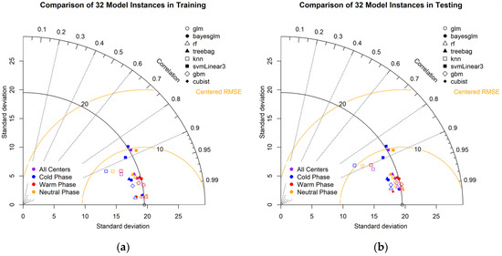
Figure 4.
Taylor diagram performance comparison of 32 model instances during the (a) training phase and (b) testing phase.
The analysis across the four phases (All Centers, Cold phase, Warm phase, and Neutral phase) shows that the model performances vary depending on the phase of the data. In the All Centers category, models tend to cluster together, indicating consistent performance across varying conditions. During the Cold phase, models like “cubist” and “rf” maintain high correlations and appropriate standard deviations, suggesting robustness in colder conditions. The Warm phase sees a slight increase in the spread of model performances, with some models like Bagged CART overestimating variability. In the Neutral phase, the model performances are more consistent, with high correlations and moderate standard deviations. Overall, models like Cubist and RF show strong, consistent performance across all phases, while others like Bagged CART exhibit more variability depending on the phase.
3.2. Cubist-Based and RF-Based Model Perfomance
The scatterplots for the Cubist models show strong performance in both training and testing phases (Figure 5a,b). In the training phase, the overall R2 value is 0.991, indicating a high degree of accuracy. The model performs slightly better during the Cold phase (R2 = 0.994) and Neutral phase (R2 = 0.991) compared to the Warm phase (R2 = 0.992). Similarly, in the testing phase, the overall R2 value is 0.979, with the Cold phase showing the highest accuracy (R2 = 0.982), followed by the Warm phase (R2 = 0.98) and the Neutral phase (R2 = 0.977). These results demonstrate the Cubist model’s robust predictive capability across different climatic phases, although there is a slight drop in performance during the testing phase compared to training.
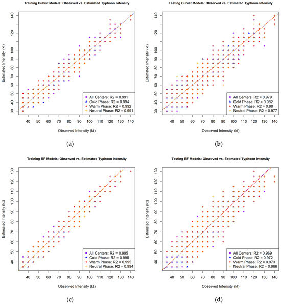
Figure 5.
Performance of (a,b) Cubist and RF (c,d) models in training and testing phases.
The scatterplots for the RF models also reflect strong performance, with slightly higher R2 values in the training phase (Figure 5c). The overall R2 value is 0.995 for training, with both Cold and Warm phases showing R2 values of 0.995 and the Neutral phase slightly lower at 0.994. In the testing phase, the overall R2 value drops to 0.969, with the Cold phase (R2 = 0.972) outperforming the Warm (R2 = 0.973) and Neutral phases (R2 = 0.966) (Figure 5d). Despite the slight decrease in R2 values during testing, the RF models exhibit good accuracy across different phases. The comparison between Cubist and RF models suggests that while both models perform well, the RF model tends to slightly outperform the Cubist model in the training phase but shows a comparable performance in the testing phase. R2 index values are also shown in detail in Table 2.
3.3. Spatial Distribution of Error Estimation
These images depict the absolute error distribution for typhoon intensity forecasts using Cubist-based models in the WNP region. Each image represents a different dataset or climatological phase used for testing the models. The blue points indicate forecast errors, with lighter shades of blue representing higher errors. Additionally, yellow and orange points highlight areas with even higher forecast errors compared to the light blue regions. In the map of the maximum absolute error of the Cubist and RF models (Figure 6a,b), which includes all tracks, the highest errors are concentrated around the Philippine archipelago, particularly the northern islands like Luzon, as well as in the South China Sea and East China Sea regions. Some yellow and orange points can be seen in these areas, indicating the most significant forecast challenges.
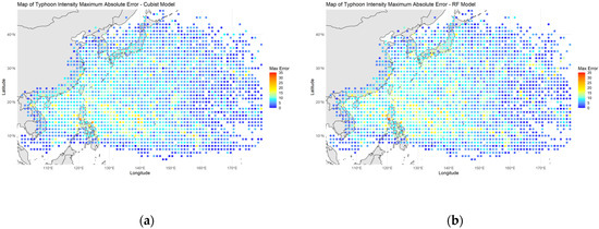
Figure 6.
Error map of Cubist and RF model testing phases with all data: (a) Cubist and (b) RF models.
Figure 7 shows error locations where values greater than 5 knots (MAE ≥ 5 kt) occur in testing across three phases of ENSO for Cubist and RF models. During the Neutral phase (Figure 7a,b), the errors are more scattered, but there are still noticeable concentrations of higher errors (lighter blues and some yellow/orange points) around the Philippines, the South China Sea, and the East China Sea. The Cold phase (Figure 7c,f) shows a high concentration of higher errors, including yellow and orange points, around the northern Philippine islands, particularly Luzon, as well as in the South China Sea and areas east of the Philippines. In the Warm phase (Figure 7b,e), the higher errors are more widespread across the WNP, with notable concentrations of light blue, yellow, and orange points around the northern Philippines, the South China Sea region, and the areas east of the Philippines towards the central Pacific.
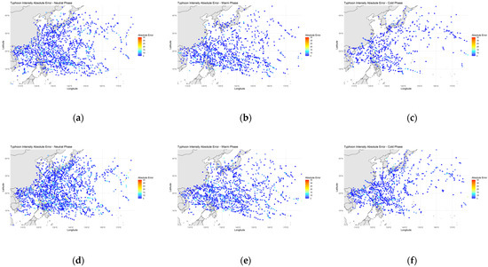
Figure 7.
Mean absolute error (MAE, ≥5 kt) in testing across three phases of ENSO for the Cubist model and RF model. Panels show: (a) Cubist model during Neutral phase, (b) Cubist model during Warm phase, (c) Cubist model during Cold phase, (d) RF model during Neutral phase, (e) RF model during Warm phase, and (f) RF model during Cold phase. The color scale is consistent across all plots to facilitate comparison.
3.4. Month-Wise Distribution of Errors
Figure 8 shows a line plot with two lines, representing two different models: “Cubist” (shown in blue) and “RF” (shown in red). The x-axis represents 12 months of the year from January to December, while the y-axis displays a range of values from around 1.5 to 2.5.
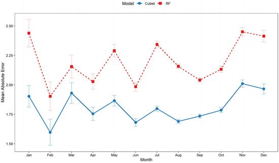
Figure 8.
Month-wise error of Cubist and RF models.
The plot does not reveal a clear seasonal pattern in the MAE, as the values oscillate monthly without a consistent trend. While initial expectations might suggest higher errors during the peak typhoon season (typically July to October), these months lie in the middle range of MAE values for the year.
For the RF model, the highest MAE is observed in January and November, with values around 2.4. The Cubist model peaks in November with an MAE around 2.0. Wider confidence intervals, like in February for Cubist, indicate higher uncertainty in error estimates. Narrower intervals, like in August for RF, suggest more consistent errors. Overall, the Cubist model consistently shows lower MAE values compared to the RF model throughout the year. Cubist’s lowest MAE of approximately 1.75 occurs in February (as shown in Figure 8).
Smaller error bars indicate higher confidence in the error estimates, while larger error bars indicate lower confidence. It is worth noting that both models show similar trends in error fluctuations, with peaks and troughs often occurring in the same months, suggesting some underlying factor affecting both models similarly.
3.5. Important Features
The boxplot visualization reveals that minimum central pressure or pressure is the most influential factor for predicting typhoon intensity, consistently ranked at the top with minimal variation. This indicates that the minimum central pressure is crucial for accurate predictions. Longitude and year follow in importance, although with moderate to high variability, suggesting their significance can differ based on specific conditions or datasets. Features like latitude, distance to land, and number show moderate importance and variability, indicating their roles are somewhat dependent on other interacting factors. The lower rankings of landfall indicator and storm direction, despite their expected significance, suggest these features might not be as critical in this model ensemble’s predictions. Features such as day, month, and storm speed are among the least important contributors, with storm speed consistently ranked low, implying it does not significantly affect intensity predictions (as shown in Figure 9).
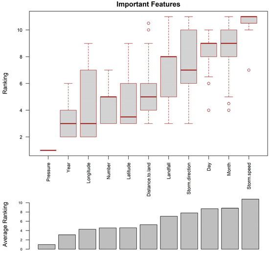
Figure 9.
Ranking of important features based on the average of 30 runs each from the Cubist and RF models, resulting in a total of 60 runs.
3.6. Comparison of Model Performance between Current and Previous Studies
The current study utilizes 32 model instances, with the top two being the Cubist and RF models combined with best-track data to estimate typhoon intensity, achieving good performance compared to a range of previous methods. Table 3 compares the performance of various models for typhoon intensity estimation over the WNP region, highlighting the RMSE values in both meters per second (m/s) and knots. It clearly shows that the current study’s ML models outperform DL networks, hybrid models, satellite-based techniques, and traditional Dvorak approaches. Specifically, the Cubist model achieves an RMSE of 1.37 ± 0.23 m/s (2.66 ± 0.04 knots), and the RF model achieves 1.66 ± 0.23 m/s (3.22 ± 0.04 knots). These lower RMSE values emphasize the effectiveness of boosting and tree-based machine learning methods in capturing the complex dynamics of typhoon intensity, offering more accurate and reliable predictions than earlier methods.

Table 3.
Comparison of model performance for typhoon intensity estimation between current and previous studies over the WNP region. Values are presented in RMSE. Bold values represent original findings from previous studies. Note: 1 m/s = 1.9438 knots.
Deep learning approaches, often utilizing satellite data, have also been explored for typhoon intensity estimation. Jiang et al. implemented a DMANet with a Kalman Filter, resulting in an RMSE of 4.02 m/s (7.82 knots) [21]. Similarly, Wang et al. [35] and Chen et al. [36] used convolutional neural networks (CNNs) with Himawari-8 geostationary satellite data, achieving RMSE values of 4.62 m/s (8.98 knots) and 4.32 m/s (8.39 knots), respectively. However, while deep learning models are powerful in handling large and complex datasets, their performance generally shows higher errors compared to the current study’s methods. Additionally, hybrid models and advanced machine learning techniques like the dynamic balance CNN by Tian et al. [37], CatBoost model by Zhong et al. [38] and the spatiotemporal interaction attention model by Zhang et al. [39] performed slightly better than standard CNN approaches but still lagged behind the current study’s models.
Other techniques for typhoon intensity estimation include methods leveraging satellite observations and traditional techniques like the Dvorak method. Studies such as those by Xiang et al. [40] and Sakuragi et al. [41] used satellite data, but their RMSE values, ranging from 5.94 to 7.27 m/s (11.55 to 14.3 knots), indicate greater estimation errors. Ritchie et al. [42] utilized the deviation-angle variance technique, yielding RMSEs of 7.27 m/s (14.3 knots). Infrared satellite image-based methods also yielded higher errors, with Zhang et al. [19], Lu and Yu [43], and Zhao et al. [44] reporting RMSE values between 6.18 and 7.30 m/s (12.01 and 14.19 knots). Traditional approaches like the ADT and its AI-enhanced variant (AiDT) still exhibit higher errors than the machine learning models used in the current study, further emphasizing the superior performance of the Cubist and RF models. Ryu et al. [45] used the ADT, reporting an RMSE of 4.39 m/s (8.53 knots). Olander et al. [18] enhanced the ADT with artificial intelligence, referred to as AiDT, improving the RMSE to 3.76 m/s (7.30 knots).
4. Discussion
The stability observed in NSE and RMSE values across training and testing datasets indicates consistent model performance without notable overfitting or underfitting issues. Specifically, models such as “cubist” and “rf” demonstrate strong and consistent performance across all phases of the data. This suggests that these models are robust and capable of generalizing well to different conditions. Overall, the results highlight the reliability of certain models like “cubist” and “rf” across various phases, while emphasizing the need for further investigation into the factors influencing the performance variability of other models.
Spatial patterns of model error highlight challenges in accurately predicting typhoon intensities around the Philippine archipelago, particularly in the northern islands, and in the South China Sea and East China Sea areas. These challenges may stem from the complex interactions between typhoons, land masses, topography, and atmospheric/oceanic conditions in these regions. Additionally, variations across different climatological phases suggest that larger-scale climate patterns or phenomena may influence model performance.
Temporally, this trend indicates the increased difficulty in accurately predicting typhoon intensities during the peak season. The lack of a clear seasonal pattern suggests that factors other than seasonality may influence the error rates for both models. Peak errors occur in January and November, which suggests that forecast models encounter greater challenges in predicting typhoon intensities during periods of intense typhoon activity. The seasonal variation in MAE may be attributed to several factors, including changes in environmental conditions (e.g., sea surface temperatures, atmospheric patterns) that influence typhoon formation and intensification, as well as the availability and quality of observational data used for model initialization and validation.
The analysis identified minimum central pressure or pressure as the most influential factor for predicting typhoon intensities, aligning with established meteorological knowledge. Central pressure serves as a critical indicator of TC intensity. Although central pressure measurements are often estimated using wind speed in methods like the Dvorak technique [3,4], they are crucial in assessing the destructive potential of a TC [46]. However, other factors like location, distance to land, and environmental conditions also contribute significantly to improving the forecast accuracy of our model. Prioritizing high-quality minimum central pressure observations and exploring interactions between central pressure and other factors could improve forecast accuracy. While features like day, month, and storm speed are among the least important contributors, further exploration is needed to understand the conditional impacts of variables like year and latitude. Future work could involve refining models to focus on high-importance features, conducting further analysis of variable features, and validating findings across different datasets to ensure robust and accurate predictions.
The current study’s use of 32 model instances, particularly the Cubist and RF models combined with best-track data, represents a significant advancement in typhoon intensity estimation. These models demonstrate better performance compared to previous methods. Specifically, the Cubist model achieves an RMSE of 1.37 ± 0.23 m/s (2.66 ± 0.04 knots) and the RF model achieves 1.66 ± 0.23 m/s (3.22 ± 0.04 knots), outperforming DL networks, hybrid models, satellite-based techniques, and traditional Dvorak approaches. Although DL methods like DMANet and CNNs show progress with RMSE values between 4.02 and 4.62 m/s (7.82 to 8.98 knots), they generally exhibit higher errors than the current study’s models. Hybrid models, such as CatBoost and spatiotemporal interaction attention models, also demonstrate improved performance over standard CNNs but do not reach the accuracy of the Cubist and RF models. Traditional and satellite-based techniques, including microwave observations, infrared images, and the Dvorak method, typically show higher RMSE values, indicating less accuracy. The Cubist and RF models make the most of the detailed best-track data, which includes key information like wind speed, pressure, and location, leading to more accurate intensity predictions. These results highlight the effectiveness of boosting and tree-based machine learning methods in accurately predicting typhoon intensity.
The main limitation of this study is its reliance solely on best-track data and domain experts for model development. Future work should explore incorporating additional data sources and methods to reduce reliance on expert judgment, enhancing the robustness and applicability of the prediction model.
5. Conclusions
This study compares 32 instances of models using an ENSO phases approach for training TC intensity estimation models, utilizing three ENSO phases (Warm, Cold, and Neutral) for comparison. We extracted best-track data of 1017 TCs throughout 1979–2020 in the WNP region, incorporating ten features from 24,485 track points. Our main findings are as follows:
- The Cubist and RF methods consistently outperform other models in both training and testing datasets. These two models, Cubist and RF, exhibit superior performance, as indicated by statistical indices. The RMSE of the best-performing algorithm (RF model during the Cold phase of ENSO) is 1.289 knots (~0.663 m/s), showcasing the potential of best-track data for intensity estimation. ENSO phases significantly impact ML model performance, potentially aiding faster learning.
- In testing phase models based on ENSO phases, the performance ranks as follows: Cubist consistently outperforms RF, followed by GBM, GLM, and Bayesian GLM, while kNN and SVM with a Linear Kernel demonstrate lower performance.
- The mean error is highest in November and lowest in February.
- During the Warm phase of ENSO, the error is greater than in other phases, especially in the South China Sea.
- Our findings indicate that minimal central pressure significantly influences TC intensity estimates, exerting the most substantial impact. Further environmental features will be incorporated to enhance the robustness of these models.
Author Contributions
Y.-A.L.: Conceptualization, Supervision and Project administration, Methodology and Formal analysis, Resources and Software, Writing—original draft, Writing—review and editing. T.-V.L.: Conceptualization, Data curation, Methodology and Formal analysis, Resources and Software, Writing—original draft, Writing—review and editing. All authors have read and agreed to the published version of the manuscript.
Funding
This research was supported in part by National Science and Technology Council of Taiwan under the Grant 113-2111-M-008-022 and Grant 113-2121-M-008-001.
Data Availability Statement
The data supporting the findings of this study are publicly available. The International Best Track Archive for Climate Stewardship (IBTrACS) data can be accessed at https://www.ncei.noaa.gov/products/international-best-track-archive (accessed on 30 November 2022). The Multivariate ENSO Index (MEI) v2 data are available at https://www.psl.noaa.gov/enso/mei/ (accessed on 1 January 2023).
Conflicts of Interest
The authors declare no conflicts of interest.
Appendix A

Table A1.
List of models used in this work.
Table A1.
List of models used in this work.
| Type of Model | Model | Package (in R) | Command Line (in R) | Hyperparameters |
|---|---|---|---|---|
| Tree-based | Random Forest (RF) | randomForest | rf | ntree = 2000 mtry = 5 |
| Bagged Classification and Regression Trees (CART) | e1071 | treebag | --- | |
| Boosting model | Gradient Boosting Machine (GBM) | gbm | gbm | n.trees = 100 interaction.depth = 1 shrinkage = 0.1 n.minobsinnode = 10 |
| Cubist | cubist | cubist | committees = 100 neighbors = 5 | |
| Instance-based | K-Nearest Neighbor (knn) | caret | knn | k = 6 |
| Support Vector Machine (SVM) | LiblineaR | svmLinear3 | cost = 1 Loss = L2 (Mean square error) | |
| Linear model | Generalized Linear Model (GLM) | caret | glm | --- |
| Bayesian GLM | arm | bayesglm | --- |
References
- IPCC. Climate Change 2021: The Physical Science Basis. In Contribution of Working Group I to the Sixth Assessment Report of the Intergovernmental Panel on Climate Change; Masson-Delmotte, V., Zhai, P., Pirani, A., Connors, S.L., Péan, C., Berger, S., Caud, N., Chen, Y., Goldfarb, L., Gomis, M.I., et al., Eds.; Cambridge University Press: Cambridge, UK, 2021. [Google Scholar]
- Pandey, R.S.; Liou, Y.-A. Typhoon strength rising in the past four decades. Weather Clim. Extrem. 2022, 36, 100446. [Google Scholar] [CrossRef]
- Dvorak, V.F. Tropical cyclone intensity analysis and forecasting from satellite imagery. Mon. Weather Rev. 1975, 103, 420–430. [Google Scholar] [CrossRef]
- Dvorak, V.F. Tropical Cyclone Intensity Analysis Using Satellite Data; National Oceanic and Atmospheric Administration, National Environmental Satellite, Data, and Information Service: Washington, DC, USA, 1984; Volume 11. [Google Scholar]
- Velden, C.; Harper, B.; Wells, F.; Beven, J.L.; Zehr, R.; Olander, T.; McCrone, P. The Dvorak tropical cyclone intensity estimation technique: A satellite-based method that has endured for over 30 years. Bull. Am. Meteorol. Soc. 2006, 87, 1195–1210. [Google Scholar] [CrossRef]
- Olander, T.L.; Velden, C.S. The advanced Dvorak technique (ADT) for estimating tropical cyclone intensity: Update and new capabilities. Weather Forecast. 2019, 34, 905–922. [Google Scholar] [CrossRef]
- Liou, Y.-A.; Liu, J.-C.; Wu, M.-X.; Lee, Y.-J.; Cheng, C.-H.; Kuei, C.-P.; Hong, R.-M. Generalized empirical formulas of threshold distance to characterize cyclone–cyclone interactions. IEEE Trans. Geosci. Remote Sens. 2016, 54, 3502–3512. [Google Scholar] [CrossRef]
- Liou, Y.-A.; Pandey, R.S. Interactions between typhoons Parma and Melor (2009) in North West Pacific Ocean. Weather Clim. Extrem. 2020, 29, 100272. [Google Scholar] [CrossRef]
- Kar, C.; Banerjee, S. An image processing approach for intensity detection of tropical cyclone using feature vector analysis. Int. J. Image Data Fusion 2018, 9, 338–348. [Google Scholar] [CrossRef]
- Finocchio, P.M.; Majumdar, S.J. The predictability of idealized tropical cyclones in environments with time-varying vertical wind shear. J. Adv. Model. Earth Syst. 2017, 9, 2836–2862. [Google Scholar] [CrossRef]
- Lee, C.Y.; Tippett, M.K.; Camargo, S.J.; Sobel, A.H. Probabilistic multiple linear regression modeling for tropical cyclone intensity. Mon. Weather Rev. 2015, 143, 933–954. [Google Scholar] [CrossRef]
- Bhattacharya, S.K.; Kotal, S.D.; Nath, S.; Bhowmik SK, R.; Kundu, P.K. Tropical cyclone intensity prediction over the North Indian Ocean-An NWP based objective approach. Geofizika 2018, 35, 189–278. [Google Scholar] [CrossRef]
- Davis, C.A. Resolving tropical cyclone intensity in models. Geophys. Res. Lett. 2018, 45, 2082–2087. [Google Scholar] [CrossRef]
- Griffin, J.S.; Burpee, R.W.; Marks, F.D.; Franklin, J.L. Real-time airborne analysis of aircraft data supporting operational hurricane forecasting. Weather Forecast. 1992, 7, 480–490. [Google Scholar] [CrossRef]
- Lee, R.S.; Lin, J.N.K. An elastic contour matching model for tropical cyclone pattern recognition. IEEE Trans. Syst. Man Cybern. Part B (Cybern.) 2001, 31, 413–417. [Google Scholar] [CrossRef] [PubMed]
- Chen, R.; Zhang, W.; Wang, X. Machine learning in tropical cyclone forecast modeling: A review. Atmosphere 2020, 11, 676. [Google Scholar] [CrossRef]
- Biswas, K.; Kumar, S.; Pandey, A.K. Tropical cyclone intensity estimations over the Indian ocean using machine learning. arXiv 2021, arXiv:2107.05573. [Google Scholar]
- Olander, T.; Wimmers, A.; Velden, C.; Kossin, J.P. Investigation of machine learning using satellite-based advanced Dvorak technique analysis parameters to estimate tropical cyclone intensity. Weather Forecast. 2021, 36, 2161–2186. [Google Scholar] [CrossRef]
- Zhang, C.J.; Luo, Q.; Dai, L.J.; Ma, L.M.; Lu, X.Q. Intensity estimation of tropical cyclones using the relevance vector machine from infrared satellite image data. IEEE J. Sel. Top. Appl. Earth Obs. Remote Sens. 2019, 12, 763–773. [Google Scholar] [CrossRef]
- Tan, J.; Yang, Q.; Hu, J.; Huang, Q.; Chen, S. Tropical cyclone intensity estimation using Himawari-8 satellite cloud products and deep learning. Remote Sens. 2022, 14, 812. [Google Scholar] [CrossRef]
- Jiang, W.; Hu, G.; Wu, T.; Liu, L.; Kim, B.; Xiao, Y.; Duan, Z. DMANet_KF: Tropical cyclone intensity estimation based on deep learning and Kalman filter from multi-spectral infrared images. IEEE J. Sel. Top. Appl. Earth Obs. Remote Sens. 2023, 16, 4469–4483. [Google Scholar] [CrossRef]
- Knapp, K.R.; Kruk, M.C.; Levinson, D.H.; Diamond, H.J.; Neumann, C.J. The international best track archive for climate stewardship (IBTrACS) unifying tropical cyclone data. Bull. Am. Meteorol. Soc. 2010, 91, 363–376. [Google Scholar] [CrossRef]
- Kursa, M.B.; Rudnicki, W.R. Feature Selection with the Boruta Package. J. Stat. Softw. 2010, 36, 1–13. [Google Scholar] [CrossRef]
- Breiman, L. Random forests. Mach. Learn. 2001, 45, 5–32. [Google Scholar] [CrossRef]
- Sutton, C.D. Classification and regression trees, bagging, and boosting. Handb. Stat. 2005, 24, 303–329. [Google Scholar]
- Friedman, J.H. Greedy function approximation: A gradient boosting machine. Ann. Stat. 2001, 29, 1189–1232. [Google Scholar] [CrossRef]
- Friedman, J.H. Stochastic gradient boosting. Comput. Stat. Data Anal. 2002, 38, 367–378. [Google Scholar] [CrossRef]
- Quinlan, J.R. Learning with Continuous Classes. In Proceedings of the 5th Australian Joint Conference on Artificial Intelligence, Hobart, Australia, 16–18 November 1992. [Google Scholar]
- Kramer, O. K-Nearest Neighbors. In Dimensionality Reduction with Unsupervised Nearest Neighbors; Springer: Berlin/Heidelberg, Germany, 2013; pp. 19–33. [Google Scholar]
- Cortes, C.; Vapnik, V. Support-vector networks. Mach. Learn. 1995, 20, 273–297. [Google Scholar] [CrossRef]
- Myers, R.H.; Montgomery, D.C. A tutorial on generalized linear models. J. Qual. Technol. 1997, 29, 274–291. [Google Scholar] [CrossRef]
- Zhao, Y.; Staudenmayer, J.; Coull, B.A.; Wand, M.P. General design Bayesian generalized linear mixed models. Stat. Sci. 2006, 21, 35–51. [Google Scholar] [CrossRef]
- Altmann, A.; Toloşi, L.; Sander, O.; Lengauer, T. Permutation importance: A corrected feature importance measure. Bioinformatics 2010, 26, 1340–1347. [Google Scholar] [CrossRef]
- Jergensen, G.E.; McGovern, A.; Lagerquist, R.; Smith, T. Classifying convective storms using machine learning. Weather Forecast. 2020, 35, 537–559. [Google Scholar] [CrossRef]
- Wang, C.; Zheng, G.; Li, X.; Xu, Q.; Liu, B.; Zhang, J. Tropical Cyclone Intensity Estimation from Geostationary Satellite Imagery Using Deep Convolutional Neural Networks. IEEE Trans. Geosci. Remote Sens. 2021, 60, 4101416. [Google Scholar] [CrossRef]
- Chen, B.F.; Chen, B.; Lin, H.T.; Elsberry, R.L. Estimating Tropical Cyclone Intensity by Satellite Imagery Utilizing Convolutional Neural Networks. Weather Forecast. 2019, 34, 447–465. [Google Scholar] [CrossRef]
- Tian, W.; Lai, L.; Niu, X.; Zhou, X.; Zhang, Y.; Lim Kam Sian, K.T.C. Estimating Tropical Cyclone Intensity Using Dynamic Balance Convolutional Neural Network from Satellite Imagery. J. Appl. Remote Sens. 2023, 17, 024513. [Google Scholar] [CrossRef]
- Zhong, W.; Zhang, D.; Sun, Y.; Wang, Q. A CatBoost-Based Model for the Intensity Detection of Tropical Cyclones over the Western North Pacific Based on Satellite Cloud Images. Remote Sens. 2023, 15, 3510. [Google Scholar] [CrossRef]
- Zhang, R.; Liu, Y.; Yue, L.; Liu, Q.; Hang, R. Estimating Tropical Cyclone Intensity Using a STIA Model from Himawari-8 Satellite Images in the Western North Pacific Basin. IEEE Trans. Geosci. Remote Sens. 2024, 62, 4101813. [Google Scholar] [CrossRef]
- Xiang, K.; Yang, X.; Zhang, M.; Li, Z.; Kong, F. Objective Estimation of Tropical Cyclone Intensity from Active and Passive Microwave Remote Sensing Observations in the Northwestern Pacific Ocean. Remote Sens. 2019, 11, 627. [Google Scholar] [CrossRef]
- Sakuragi, T.; Hoshino, S.; Kitabatake, N. Development and Verification of a Tropical Cyclone Intensity Estimation Method Reflecting the Variety of TRMM/TMI Brightness Temperature Distribution. RSMC Tokyo-Typhoon Cent. Tech. Rev. 2014, 16, 15. [Google Scholar]
- Ritchie, E.A.; Wood, K.M.; Rodríguez-Herrera, O.G.; Piñeros, M.F.; Tyo, J.S. Satellite-Derived Tropical Cyclone Intensity in the North Pacific Ocean Using the Deviation-Angle Variance Technique. Weather Forecast. 2014, 29, 505–516. [Google Scholar] [CrossRef]
- Lu, X.; Yu, H. An Objective Tropical Cyclone Intensity Estimation Model Based on Digital IR Satellite Images. Trop. Cyclone Res. Rev. 2013, 2, 233–241. [Google Scholar]
- Zhao, Y.; Zhao, C.; Sun, R.; Wang, Z. A Multiple Linear Regression Model for Tropical Cyclone Intensity Estimation from Satellite Infrared Images. Atmosphere 2016, 7, 40. [Google Scholar] [CrossRef]
- Ryu, S.; Hong, S.E.; Park, J.D.; Hong, S. An Improved Conversion Relationship between Tropical Cyclone Intensity Index and Maximum Wind Speed for the Advanced Dvorak Technique in the Northwestern Pacific Ocean Using SMAP Data. Remote Sens. 2020, 12, 2580. [Google Scholar] [CrossRef]
- Knaff, J.A.; Zehr, R.M. Reexamination of tropical cyclone wind–pressure relationships. Weather Forecast. 2007, 22, 71–88. [Google Scholar] [CrossRef]
Disclaimer/Publisher’s Note: The statements, opinions and data contained in all publications are solely those of the individual author(s) and contributor(s) and not of MDPI and/or the editor(s). MDPI and/or the editor(s) disclaim responsibility for any injury to people or property resulting from any ideas, methods, instructions or products referred to in the content. |
© 2024 by the authors. Licensee MDPI, Basel, Switzerland. This article is an open access article distributed under the terms and conditions of the Creative Commons Attribution (CC BY) license (https://creativecommons.org/licenses/by/4.0/).