Rapid Prediction of the Lithium Content in Plants by Combining Fractional-Order Derivative Spectroscopy and Wavelet Transform Analysis

Abstract

Quickly determining the metal content in plants and subsequently identifying geochemical anomalies can provide clues and guidance for predicting the location and scale of concealed ore bodies in vegetation-covered areas. Although visible, near-infrared and shortwave infrared (VNIR–SWIR) reflectance spectroscopy at wavelengths ranging from 400 to 2500 nm has been proven by many researchers to be a fast, accurate and nondestructive approach for estimating the contents of copper (Cu), lead (Pb), zinc (Zn) and other metal elements in plants, relatively few studies have been conducted on the estimation of lithium (Li) in plants. Therefore, the potential of applying VNIR–SWIR spectroscopy techniques for estimating the Li content in plants was explored in this study. The Jingerquan Li mining area in Hami, Xinjiang, China, was chosen. Three sampling lines were established near a pegmatite deposit and in a background region, canopy reflectance spectra were obtained for desert plants and Li contents were determined in the laboratory; then, quantitative relationships were established between nine different transformed spectra (including both integer and fractional orders) and the Li content was estimated using partial least squares regression (PLSR). The results showed that models constructed using high-order derivative spectra (with an order greater than or equal to 1) significantly outperformed those based on original and low-order derivative spectra (with an order less than 1). Notably, the model based on a 1.1-order derivative spectrum displayed the best performance. Furthermore, the performance of the model based on the two-layer wavelet coefficients of the 1.1-order derivative spectrum was further improved compared with that of the model based on only the 1.1-order derivative spectrum. The coefficient of determination ($R_{pre}^2$) and the ratio of performance to deviation (RPD) for the validation set increased from 0.6977 and 1.7656 to 0.7044 and 1.8446, respectively, and the root mean square error (RMSEpre) decreased from 2.5735 to 2.4633 mg/kg. These results indicate that quickly and accurately estimating the Li content in plants via the proposed spectroscopic analysis technique is feasible and effective; however, appropriate spectral preprocessing methods should be selected before hyperspectral estimation models are constructed. Overall, the developed hybrid spectral transformation approach, which combines wavelet coefficients and derivative spectra, displayed excellent application potential for estimating the Li content in plants.

1. Introduction

Lithium (Li) and its compounds have attracted worldwide attention because of its excellent characteristics, broad range of application and high strategic value in military and civilian fields, such as in high-energy batteries, grease, ceramics, glass, fuel, catalysts, medical devices, radiation dosimeters, nuclear reactor coolants and nuclear weapons [1,2,3,4]. Li has even been called “the energy metal of the 21st century”, “the new energy upstart of the 21st century” and “the metal that drives the world forward”. The United States listed Li resources among the 43 crucial mineral resources in 2017 for the first time. The European Union listed Li as one of 14 critical raw materials in 2018. In 2019, Li was listed as one of 24 critical minerals in Australia. China also listed Li as one of 24 national strategic mineral resources [5,6,7]. With the rapid development of Li batteries and new energy vehicles in recent years, the demand for Li metals has significantly increased [4,8,9,10,11,12]. However, at present, the slow exploration of Li mineral resources has made it difficult for the supply of these resources to meet the growing market demand, and resource shortage problems have become increasingly severe [13]. Consequently, there is a pressing need to accelerate the development of innovative techniques and technologies to facilitate the exploration of lithium deposits.

As a new noncontact and long-distance spatial exploration technology, remote sensing technology has scale, cost and speed advantages over traditional geological survey methods. Notably, data can be collected at large scales, and metallogenic information can be obtained in harsh environments that are difficult for humans to access; consequently, remote sensing has become a new and effective prospecting technique globally [14]. In recent years, with the successful launch of an increasing number of sensors with high spatial and spectral resolutions and the constant maturation of data processing algorithms, remote sensing technology has rapidly developed. Therefore, an increasing number of researchers have explored Li mineral resources via remote sensing technology and have established and verified many effective exploration models. The relevant research findings can be broadly classified into two main categories: (1) the direct identification of Li minerals [7,9,11,13,15,16,17,18,19,20,21,22] and (2) the identification of hydrothermal alteration minerals that are commonly associated with Li-bearing pegmatites [23,24]. For the first category, several multispectral and hyperspectral remote sensing datasets, such as ASTER, Sentinel-2, Landsat 5, Landsat 8, and ASD FieldSpec and WorldView-2, are integrated with techniques including RGB combination, band ratio, principal component analysis (PCA), spectral angle mapper (SAM), support vector machine (SVM), mixture-tuned matched filter (MTMF), artificial neural network (ANN), random forest (RF) and spectral signature analysis to establish spectral identification markers that are capable of differentiating Li-bearing pegmatite from non-Li pegmatite, surrounding rock formations and other geological materials. The developed model can subsequently be applied to remote sensing images to achieve the rapid and accurate delineation of Li-bearing pegmatites over large areas, and relevant information can be extracted. For the second category, ASTER and Landsat 8 multispectral remote sensing data are combined with three approaches, the SAM, maximum likelihood (ML) and k-means clustering methods, to extract hydrothermal alteration minerals associated with Li-bearing pegmatites, thus providing clues and guidance for Li deposit exploration. Researchers have established various prospecting methods for Li deposits by using remote sensing technology, and these methods have yielded good application results. However, the currently used recognition models are applicable mainly to outcrops and shallow mines. When applied in vegetation-covered areas, these models often yield low recognition accuracy because of the barriers and interference associated with vegetation [13]. At present, effective prospecting methods and techniques for identifying concealed Li deposits in vegetation-covered areas are scarce. In contrast, the possibility of discovering new hidden orebodies in vast areas covered by vegetation is very high, but effective methods must be developed to identify these bodies.

In plant geochemical investigations, chemical analyses of plant ash are used to identify geochemical anomalies and metallogenic targets, effectively leveraging vegetation as an information source for economical and insightful mineral exploration, even in areas with thick weathered sediments [25,26]. As a result, an increasing number of researchers have attempted to utilize plant geochemical methods for hidden-mineral exploration in vegetation-covered areas, and many plants that can be used for the delineation of concealed ore bodies have been identified; these plants are called effective indicator plants [27,28,29,30,31,32,33,34,35,36,37,38]. However, accurately and quickly determining the metal content in indicator plants during phytochemical exploration is a considerable challenge. Although traditional laboratory chemical analysis methods for determining the metal content are accurate, they are often time-consuming and require significant labor due to extensive sample preparation and multiple analysis steps [39,40,41]. In contrast, over the past few years, numerous researchers have presented compelling evidence suggesting that hyperspectral reflectance spectroscopy is a quick, noninvasive and precise technique for estimating the metal content in plants. Three main types of spectral parameters, namely, the characteristic wavelength bands [25,41,42,43,44], vegetation indices [40,45,46,47,48,49,50] and red edge positions [51,52,53,54,55], are used to construct quantitative models for estimating the metal content in plants.

To date, few studies have utilized hyperspectral techniques to estimate the Li content in plants, particularly those growing in wild environments. In contrast, numerous studies have shown that Li in the soil is easily transported to plants via potassium (K⁺) transport pathways [2]. The common indicators of Li uptake in plants include chlorosis (yellowing of leaves), leaf curling, development of necrotic spots, reduced biomass, and a noticeable effect on the chlorophyll and water contents [2,3,56,57,58,59]. The chlorophyll and water contents significantly influence the reflectance spectra of plants in the visible and mid-infrared ranges, respectively. Thus, it is possible that there is a quantitative relationship between the reflectance spectra of plants in these two ranges and the Li content. By analyzing spectral patterns, researchers can potentially establish a correlation between specific spectral features and the concentration of Li in plants.

Therefore, the ultimate goal of this study was to investigate whether the proximal reflectance spectra of widely distributed arid desert plants can serve as a potential basis for estimating the Li content within these plants. If successful, this approach could aid in delineating target areas with high Li contents, which would be valuable for the exploration of concealed Li deposits. This research has the potential to expand the exploration space, enhance the exploration efficiency and expedite the discovery of Li resources. To achieve this goal, the following objectives were outlined: (1) to evaluate the performance of quantitative models for estimating the plant Li content via the fractional and integer derivative spectra of various orders, with the goal of identifying the optimal order, and (2) to develop estimation models that integrate derivative spectral analysis with wavelet transform and assess whether this combined spectral transformation approach yields better model performance than derivative spectral analysis method alone.

2. Materials and Methods

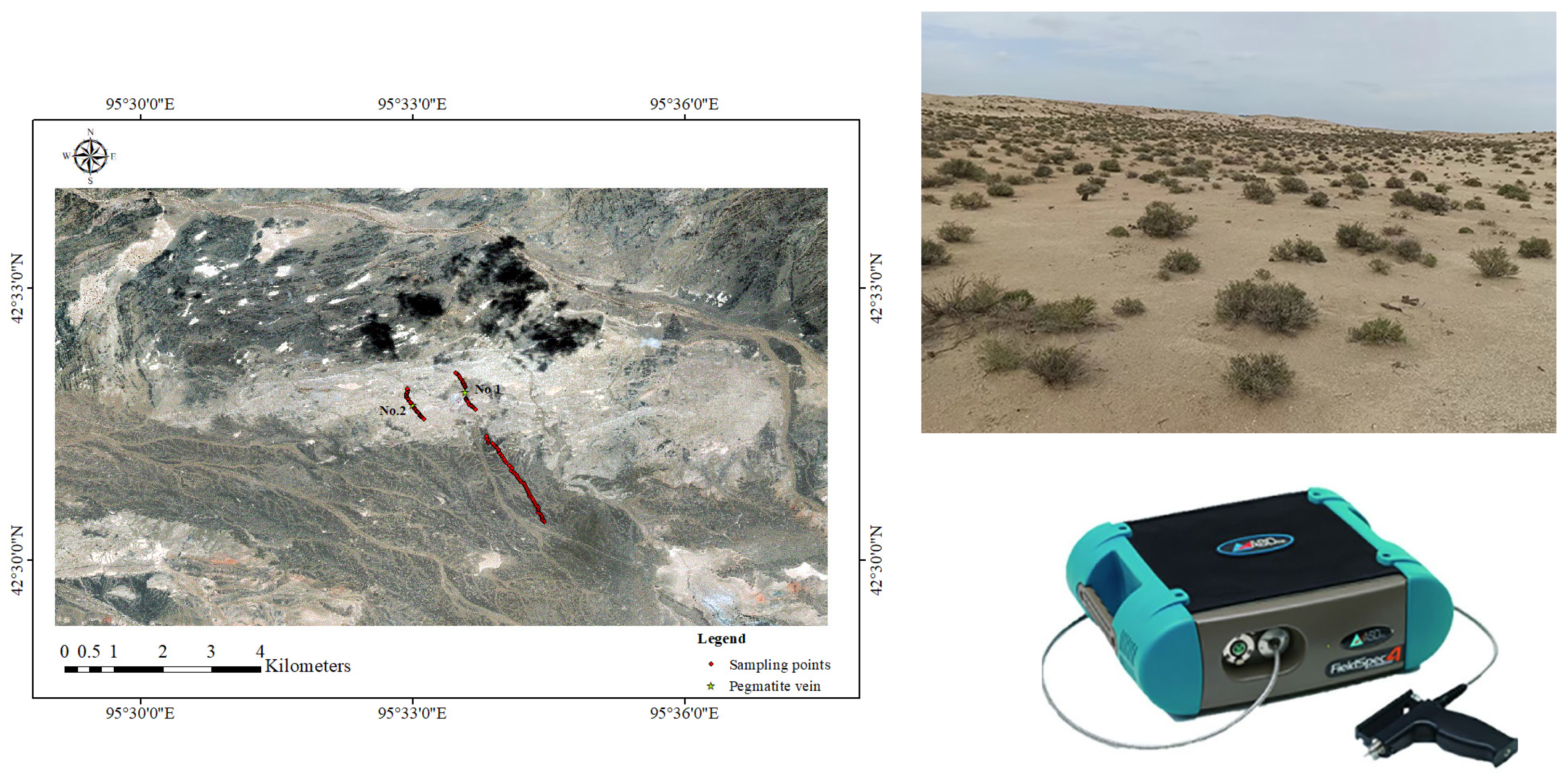
2.1. Study Area and Sampling

In this study, the research area selected was the Jingerquan Li mine area, which is located in the Hami region of Xinjiang, China. This specific area is situated approximately 170 km east of Hami city. The granite exposed in the mining area is mainly biotite granite, two-mica granite and muscovite granite, and the relationships among them are transitional and gradual [60]. Pegmatite generally occurs in the bodies of muscovite granite in mining areas, and there is a direct transition relationship between pegmatite and muscovite granite [60]. Two relatively large pegmatite dikes, no. 1 and no. 2, have been discovered (Figure 1), both of which strike in the NE–SW direction [60,61].

To investigate the spatial coupling relationship between the plant Li content and the ore body, three sampling lines were initially established. These lines were strategically positioned near the ore body and in the background area, which is distant from the ore body. Figure 1 provides a visual representation of the placement of the sampling lines. A plant with a large canopy was subsequently selected near each sampling site along the sampling lines to obtain spectral measurements. Finally, the whole plant, except for the root system, was collected to determine the Li content via inductively coupled plasma atomic emission spectrometry (ICP–AES) in the laboratory after a series of pretreatments, such as cleaning, cutting, drying and crushing. The measurement method employed in this study adhered to the constraints of the regional geochemical sample analysis method published by the People’s Republic of China in 2016 (DZ/t0279.2-2016). To maintain precise documentation of the sampling points, a handheld global positioning system (GPS) device (Garmin Inc., Olathe, KS, USA) was utilized.

2.2. Spectral Measurements and Preprocessing

A portable spectrometer, specifically, the ASD FieldSpec4 (Malvern Panalytical Ltd., Malvern, UK, formerly Analytical Spectral Devices Inc., Westborough, MA, USA), with a probing view field angle of 25 degrees was used to measure the reflectance spectra of the plant canopy. The probe of the spectrometer was positioned 15 cm above the top of the canopy. The collected plant spectra spanned from 350 to 2500 nm, with spectral bands spaced at 1 nm intervals. To ensure the quality of the spectral curves and minimize the impacts of instrument variability, random noise and measurement errors, a specific procedure was followed. Initially, five reflectance spectra were collected from the plants at each sampling point. Subsequently, any spectra showing significant differences were eliminated from the analysis. Finally, the average of the remaining spectra was calculated, resulting in a representative plant reflection spectrum for that specific sampling point.

The reflectance spectra of plants below 400 nm and above 2500 nm were removed because of the high noise level of the instrument [62]. Spectral anomalies occur between 1300 and 1399 nm and between 1800 and 2000 nm due to strong atmospheric water vapor interference, with values greater than 1 in some spectral bands. As a result, the spectra in both ranges were removed. In addition, the plant spectra were resampled using the mean over 10 adjacent wavelength bands to eliminate hyperspectral data redundancy and autocorrelation issues between spectral bands.

Removing spectral outliers from collected plant samples is crucial. Spectral outliers can significantly impact the predictive performance of an estimation model [63,64]. A total of 23 plant samples were identified as spectral outliers via the Monte Carlo outlier detection (MCOD) method in MATLAB R2017b software. The detection package for MCOD can be easily downloaded from the website http://www.libpls.net/download.php, accessed on 10 March 2023. The abnormal plant samples were removed and not used in subsequent estimation model construction. Figure 2 displays the reflectance spectra of the remaining plant samples.

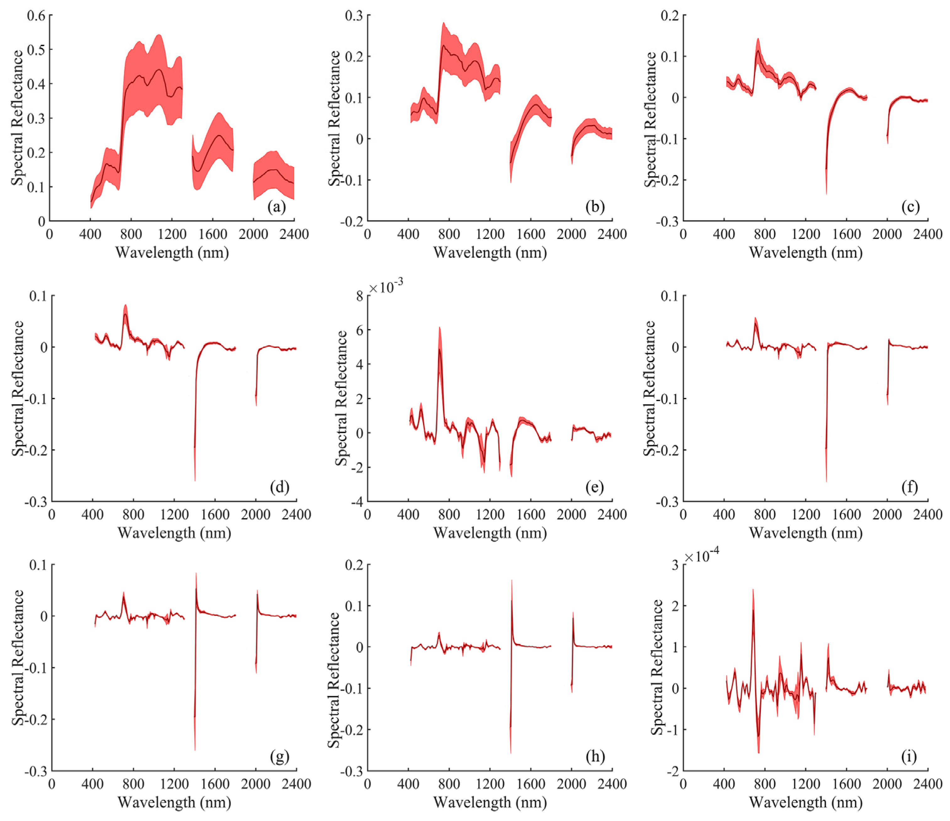
2.3. Spectral Transformation

Spectral transformation is a widely employed technique for the spectral analysis of vegetation and involves the use of mathematical methods to process and analyze spectral data. Its purpose is to enhance small spectral features that may be concealed within a spectrum and eliminate both random and instrumental noise [65,66,67]. In this study, derivative transformations, including integer (first and second) and fractional derivatives, were adopted to process the plant spectra before establishing the estimation model. To calculate the first and second derivatives in a plant spectrum composed of discrete points, the difference method was employed. The formulas for computing the first and second derivatives are provided below. Formula (1) is used for calculating the first derivative, and Formula (2) is used for calculating the second derivative.

$${\rho }^{\prime }({\lambda }_i)={\displaystyle \frac{\rho ({\lambda }_{i+1})-\rho ({\lambda }_{i-1})}{{\lambda }_{i+1}-{\lambda }_{i-1}}}$$

(1)

$${\rho }^{″}({\lambda }_i)={\displaystyle \frac{{\rho }^{\prime }({\lambda }_{i+1})-{\rho }^{\prime }({\lambda }_{i-1})}{{\lambda }_{i+1}-{\lambda }_{i-1}}}$$

(2)

where $\rho ({\lambda }_{i+1})$ and $\rho ({\lambda }_{i-1})$ represent the reflectances at wavelengths ${\lambda }_{i+1}$ and ${\lambda }_{i-1}$, respectively; ${\rho }^{\prime }({\lambda }_{i+1})$ and ${\rho }^{\prime }({\lambda }_{i-1})$ represent the first derivatives at wavelengths ${\lambda }_{i+1}$ and ${\lambda }_{i-1}$, respectively; and ${\rho }^{\prime }({\lambda }_i)$ and ${\rho }^{″}({\lambda }_i)$ represent the first and second derivatives at wavelength ${\lambda }_i$, respectively.

As a supplement to and extension of the integer-order differential, the fractional-order differential is widely used in hyperspectral data analysis because it can be used to refine the local information within hyperspectral data, effectively eliminate noise and output detailed information [68,69]. In this study, the fractional-order derivative was calculated via the Grünwald–Letnikov method, and the corresponding equation is shown in Formula (3); this approach is characterized by simplicity and high calculation efficiency [70]. Six fractional-order derivatives were calculated with an order starting at 0.2 and ending at 1.7 at an interval of 0.3.

$${\displaystyle \frac{d^{v}f(\lambda )}{d{\lambda }^v}}\approx f(\lambda )+(-V)f(\lambda -1)+{\displaystyle \frac{(-V)(-V+1)}{2}}f(\lambda -1)+...{\displaystyle \frac{\Gamma (-V+1)}{n!\Gamma (-V+n+1)}}f(\lambda -n)$$

(3)

where $V$ is the fractional derivative order; $f(\lambda ),f(\lambda -1)$ and $f(\lambda -n)$ are the spectral values of the $\lambda$, $\lambda -1$ and $\lambda -n$th wavelength bands, respectively; n is the difference between the upper and lower limits of the differential; and $\Gamma$ represents the gamma function.

2.4. Partial Least Squares Regression

PLSR, a linear multivariate regression method, was initially proposed by Wold et al. (2001) [71] and has since gained considerable popularity. Hyperspectral models based on the PLSR method can reduce the redundancy of spectral information, solve multiple correlative problems among wavelength bands and fully consider beneficial spectral information to improve the interpretability of model results [72,73,74,75,76]. Given these advantages, the PLSR method was used in this study to develop a hyperspectral model for estimating the Li content in plants.

It is essential to determine the number of principal components when the PLSR method is used to construct a hyperspectral estimation model. If this number is too small, due to the inability to fully use spectral information, the accuracy of the model will be low. In contrast, if this number is too large, the model will be too complex, and the phenomenon of overfitting may lead to poor model prediction accuracy, robustness and generalizability. The optimal number of principal components was determined in this study by assessing the coefficient of determination (R²) between the measured and predicted values. This assessment was performed via the leave-one-out cross-validation method. The ultimate objective was to maximize the R² value of the estimation model constructed with the optimal number of principal components. This approach ensured that the prediction model achieved the highest possible accuracy and precision

2.5. Wavelet Transform Method

The wavelet transform, introduced by J. Morlet in 1984 [77], enhances the Fourier transform by using a variable time–frequency window, supporting the effective localization of both high- and low-frequency information. Currently, this approach is widely used for spectral data analysis, noise reduction and refined information extraction. In wavelet transform analysis, two primary methods are commonly utilized: the discrete wavelet transform (DWT) and the continuous wavelet transform (CWT) [69]. Compared with CWT, DWT is more straightforward and effectively addresses the issue of collinearity [70]. Consequently, DWT was chosen to process the plant spectra in this study. Additionally, db7 was chosen as the wavelet basis for the scale function because the corresponding wavelet shape is similar to that of the plant spectra. The derivative spectrum is decomposed into five layers using the wavelet basis functions, resulting in the extraction of wavelet coefficients for each layer. These wavelet coefficients are then combined with the PLSR method to develop a quantitative estimation model for Li content.

2.6. Model Establishment and Accuracy Evaluation

To evaluate the effectiveness of the developed hyperspectral estimation model, the 94 collected plant samples were initially divided randomly into a calibration set comprising 69 plant samples and a validation set comprising 25 plant samples. Next, the PLSR method was employed to construct a quantitative model using the plant spectra from the calibration set for estimating the Li content. The constructed estimation model was subsequently applied to process the validation set for Li content prediction. The performance of the model was evaluated via various metrics, such as the coefficient of determination ($R_{pre}^2$), the ratio of performance to deviation (RPD) and the root mean square error (RMSEpre). In general, a model that yields high $R_{pre}^2$ and RPD values and a low RMSEpre is considered to perform well. This model provides high prediction accuracy and strong generalizability and robustness. For RPD, the following evaluation criteria proposed by Viscarra Rossel et al. (2006) were adopted in this study: RPD ≥ 2.5 (excellent model), 2.0 ≤ RPD < 2.5 (very good model), 1.8 ≤ RPD < 2.0 (good model), 1.4 ≤ RPD < 1.8 (fair model) and RPD < 1.4 (unsuccessful model).

2.7. Kruskal–Wallis Test

The Kruskal–Wallis test is a nonparametric statistical method employed to assess whether there are differences in the overall distribution of two or more independent samples. This technique does not rely on the assumption of a specific data distribution, making it applicable in scenarios where the data may not adhere to a normal distribution or when sample sizes are small. In this study, this method is primarily used to determine whether there is a significant difference in the Li content in plants between the calibration set samples and the validation set samples.

3. Results

3.1. Statistical Analysis of the Li Content in Plants

The descriptive statistical results for the measured Li contents in the plant samples are presented in

Table 1. Descriptive statistics for the Li content in the plant samples.

Dataset	Number	Min (mg/kg)	Max (mg/kg)	Mean (mg/kg)	SD (mg/kg)	CV (%)
Whole dataset	94	0.84	22.60	4.94	4.06	82.19
Calibration dataset	69	0.86	22.60	4.86	3.90	80.25
Validation dataset	25	0.84	19.11	5.14	4.54	88.32

SD: standard deviation; CV: coefficient of variation.

. The table reveals a significant variation in the plant Li content, ranging from 0.84 mg/kg to 22.6 mg/kg, with average and standard deviation (SD) values of 4.94 and 4.06 mg/kg, respectively. The range between the maximum and minimum values of the plant Li content is substantial, with an order of magnitude difference. Additionally, a calculated coefficient of variation (CV) exceeding 80% confirms a substantial level of variability within the data, strongly indicating an inhomogeneous and nonrandom distribution of the Li content in plants within the study area. Thus, the Li content in some areas was much greater than that in others, reflecting the presence of geochemical anomalies. Further statistical analysis revealed that most geochemically rich areas are close to pegmatite veins, as shown in Figure 1. The above results indicate that an abnormal Li content in plants can be used as an indicator of hidden Li ore bodies.

As shown in Table 1, the minimum, maximum, mean and standard deviation (SD) values for the Li content in the plant samples in the calibration dataset were similar to those in the validation dataset. The p value produced via the Kruskal–Wallis test between the calibration and validation datasets was 0.8574. The p value was significantly greater than 0.05, indicating that there was no significant difference in the Li content in the plant samples from the calibration and validation datasets. Therefore, data from the validation dataset can be used to assess the performance of the model constructed with data from the calibration dataset.

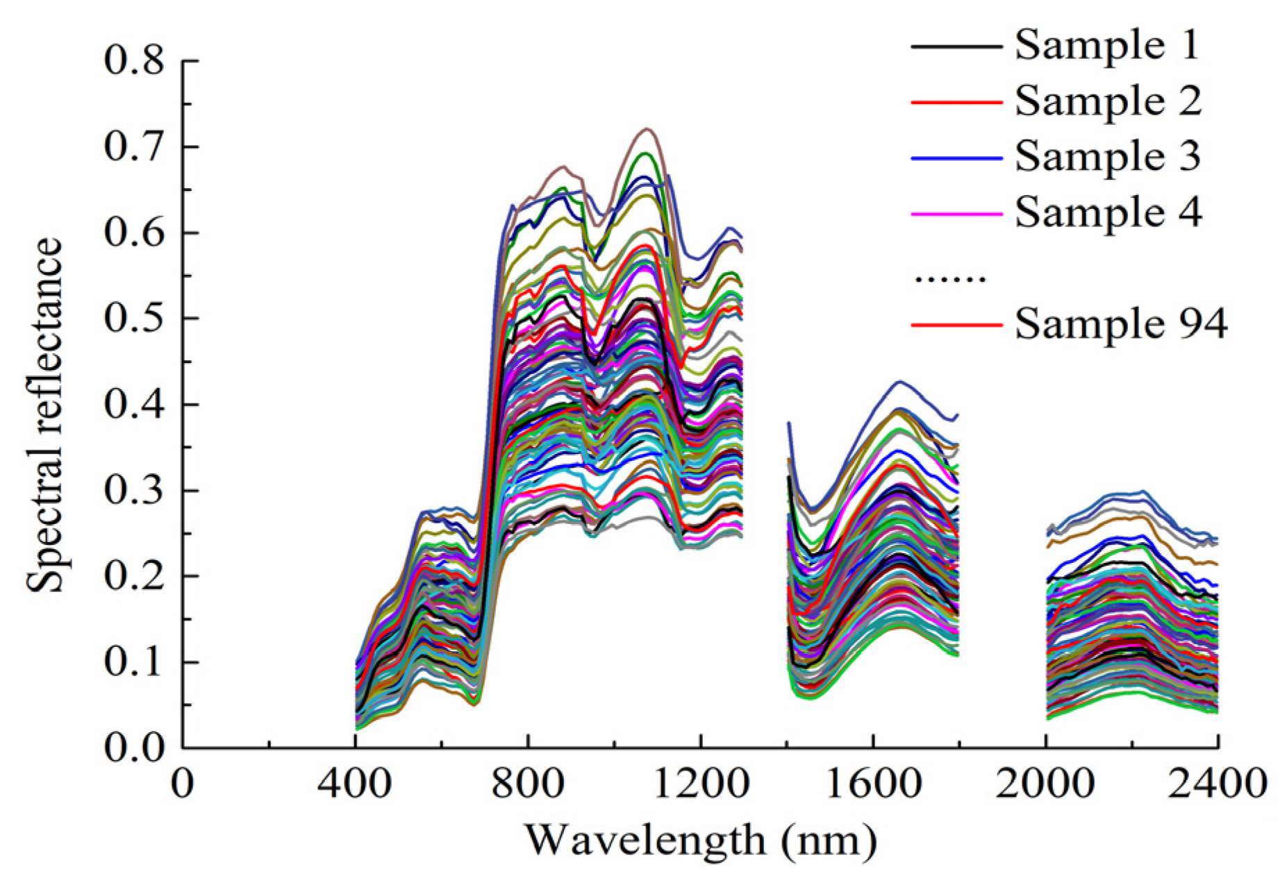
3.2. Spectral Characteristics

The average spectral curves for 69 plant samples in the calibration dataset under different spectral transformations are displayed in Figure 3. Notably, the original reflectance spectrum included one reflection peak (564.5 nm) and one absorption valley (674.5 nm) in the visible region, and the reflectance level increased rapidly from 704.5 to 884.5 nm until it reached a local maximum (0.424). The spectral reflectance remained at a high level above 0.36 within the range of 804.5 to 1294.5 nm, with two distinct absorption valleys at 954.5 and 1194.5 nm. In contrast, the reflectance was small overall in the range of 1294.5 to 2395.5 nm, with a value less than 0.3 in most spectral wavelength bands. However, there were two obvious reflection peaks and an absorption valley in this range at wavelengths of 1664.5, 2215.5 and 1454.5 nm.

Figure 3a shows that the standard deviation of the spectral values across all the wavelength bands within the range of 404.5 to 2395.5 nm is relatively high under varying Li contents, ranging from 0.0192 to 0.102, with an average value of 0.066. This indicates the challenges associated with extracting significant subtle spectral features from the original spectra, attributed to the considerable overlap and variation in their absorption ranges and waveform shapes. In contrast, Figure 3b–i shows that the variation range of most wavelength bands in the derivative spectra decreased and gradually approached 0 as the order increased. The average standard deviations of the 0.2, 0.5, 0.8, 1, 1.1, 1.4, 1.7 and 2nd derivatives across all the bands for different Li contents are 0.028, 0.009, 0.004, 0.00002, 0.0027, 0.0027, 0.0028 and 0.00001, respectively. These values are significantly lower than the value of 0.066 observed in the original spectra. This indicates that the spectral baseline drift and overlapping peaks were gradually removed. As the derivative order increased, the existing spectral characteristics became increasingly obvious, especially the red edge features in the wavelength range of 674.5 to 764.5 nm. Additionally, new absorption valleys and reflection peaks emerged, particularly at wavelengths of approximately 484.5, 814.5, 894.5, 934.5 and 1144.5 nm (as shown in Figure 3b–i).

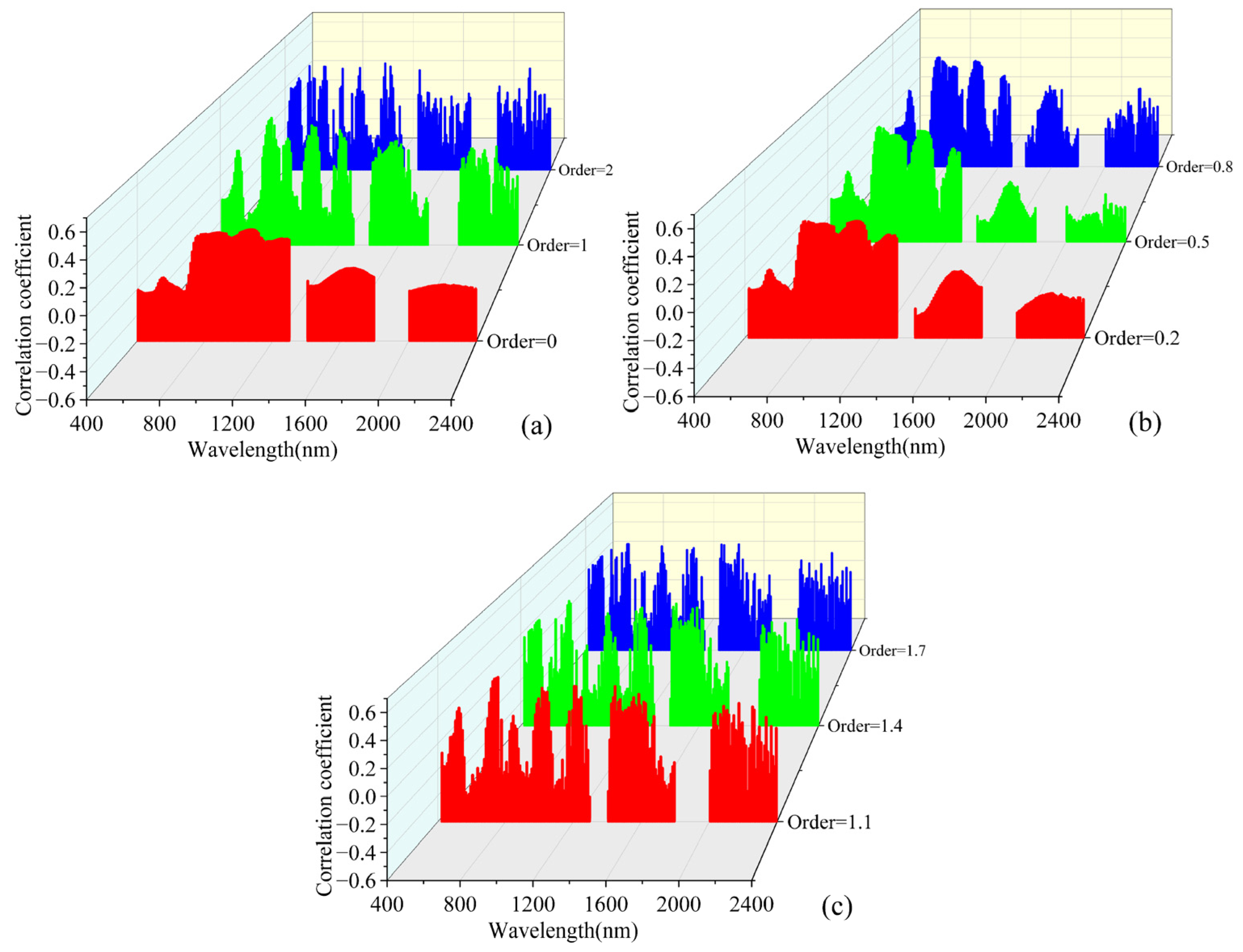
3.3. Correlation Analysis between the Transformed Spectra and the Li Content

The correlation coefficients between the different types of transformation spectra in the range of 404.5 to 2395.5 nm and the Li contents of the plant samples in the calibration dataset were calculated and plotted, as shown in Figure 4. The original reflectance spectra ranging from 404.5 to 714.5 nm were negatively correlated with the Li content, with correlation coefficients varying between −0.233 and −0.003. This negative correlation reached a local maximum, forming two peaks at 454.5 and 674.5 nm. However, the overall correlation was low, with the maximum absolute value of the correlation coefficient (|r|) reaching only 0.233. Additionally, the |r| value increased rapidly from 714.5 nm to a local maximum of 894.5 nm. The original reflectance spectra between wavelengths of 894.5 and 1294.5 nm exhibited a positive correlation with the Li content of the plant samples. The correlation was strongest at 1074.5 nm, with an |r| value of 0.256. In contrast, the correlation was weakly negative in the ranges of 1404.5 to 1794.5 and 2005.5 to 2395.5 nm. Within these ranges, the correlation was strongest at 1434.5 nm, but the |r| value did not exceed 0.19.

Overall, the correlation coefficients between the spectral values of the original spectra in the 404.5 to 2395.5 nm range and the Li content were relatively low, with |r| remaining below 0.3. Additionally, the correlation tended to vary smoothly across different wavelengths. In contrast, the correlation coefficient of the derivative spectra, whether for integer or fractional derivatives, closely varied with wavelength, and the amplitude of the fluctuations increased significantly, even in cases with significant differences between adjacent wavelength bands (Figure 4a–c). In general, the correlation between the derivative spectra and Li content was stronger than that between the original spectra and the Li content. The average |r| value for all wavelength bands within the 404.5 to 2395.5 nm range in the original spectrum is 0.17, whereas the average |r| value for the derivative spectrum falls between 0.21 and 0.27. Notably, many peaks appeared in the curve of the correlation coefficient between the derivative spectra and Li content, especially at wavelengths of 744.5, 1044.5, 1194.5, 1444.5 and 1584.5 nm. Therefore, compared with the original spectra, the derivative spectra more effectively represent the characteristics of the spectral bands, making them more suitable for building a hyperspectral model to quantitatively estimate the Li content in plants.

Figure 4 shows that, as the order of the derivative continued to increase, many positive and negative peaks occurred. Compared with that for the low-derivative spectra (order less than 1), the correlation between the high-derivative spectra (order greater than or equal to 1) and the Li content obviously increased, especially in the wavelength range of 1404.5 to 1794.5 nm. In this wavelength range, the |r| value between the low-order derivative spectra and Li content was less than 0.2, and that for the high-order derivative spectra was greater than 0.23; additionally, at some wavelengths, such as 1444.5, 1554.5 and 1584.5 nm, these values were even greater than 0.4. Figure 4 also shows that the fractional-order derivative spectra (those with an order greater than 1) yielded stronger correlations between some specific spectral bands and the Li content in plants than did the integer derivative spectra. For example, the |r| value was the highest at 754.5 nm for the 1.1-order derivative spectrum, reaching 0.51, compared with 0.33 and 0.49 for the first- and second-order derivative spectra, respectively.

Overall, the correlation analysis provided a theoretical basis for establishing a quantitative estimation model of the Li content in plants via spectroscopy information for subsequent analysis.

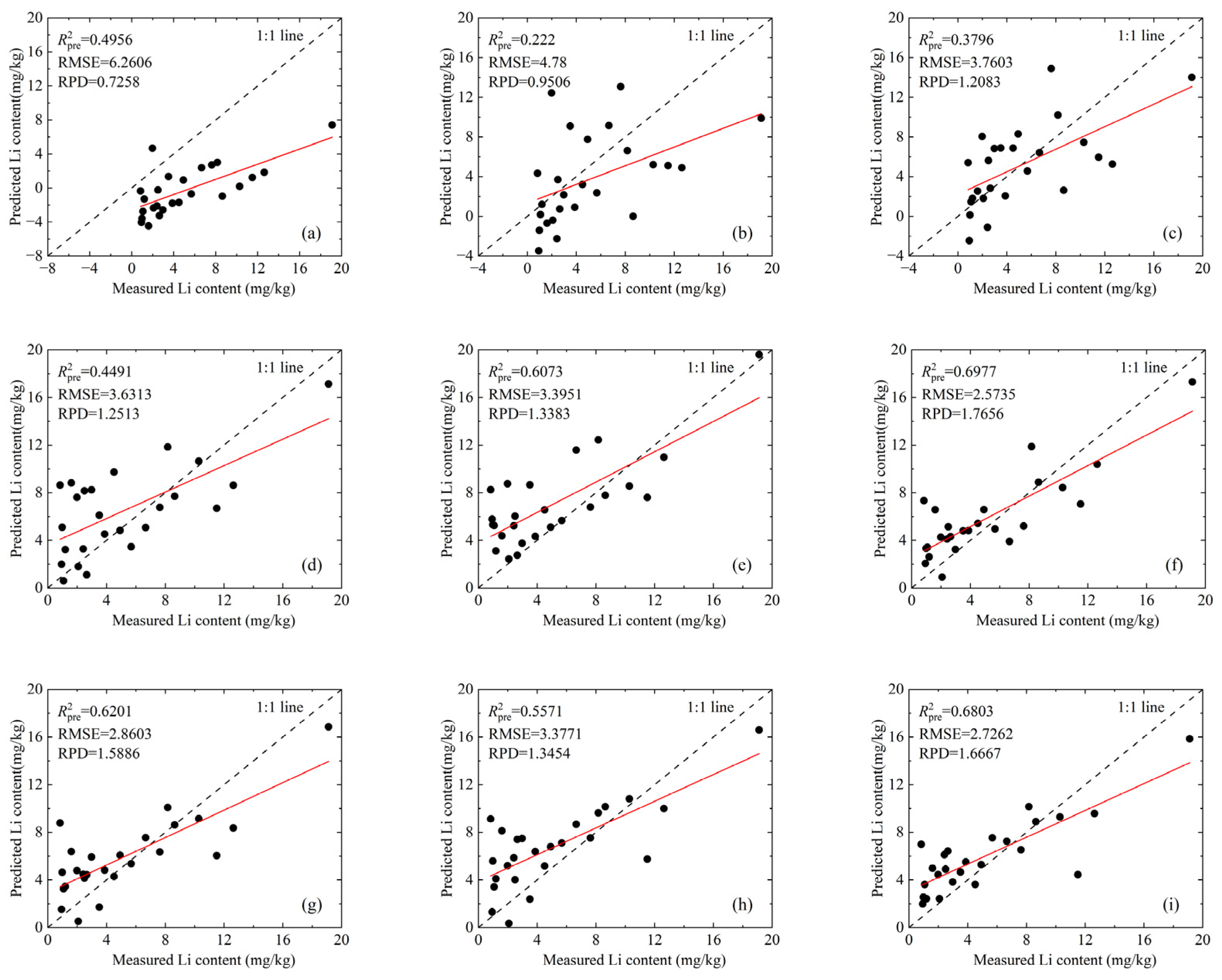
3.4. Establishment of the Estimation Model

To assess the impact of various spectral transformation methods on the estimation of the Li content in plants and to identify the most effective transformation spectrum, the performance of the quantitative hyperspectral estimation model was evaluated based on different forms of transformation spectra.

Table 2. Comparison of the prediction accuracy and ability of models based on different transform spectra.

Spectral Transformation Form	Number of Principal Components	Calibration Set		Validation Set
		${\mathit{R}}_{\mathit{c}}^{\mathbf{2}}$	RMSEc (mg/kg)	${\mathit{R}}_{\mathit{p}\mathit{r}\mathit{e}}^{\mathbf{2}}$	RMSEpre (mg/kg)	RPD
Order = 0	9	0.5897	2.4784	0.4956	6.2606	0.7258
Order = 0.2	9	0.6939	2.1407	0.222	4.78	0.9506
Order = 0.5	8	0.678	2.1955	0.3796	3.7603	1.2083
Order = 0.8	8	0.7639	1.8798	0.4491	3.6313	1.2513
Order = 1	6	0.6903	2.1531	0.6073	3.3951	1.3383
Order = 1.1	5	0.6583	2.2616	0.6977	2.5735	1.7656
Order = 1.4	5	0.6944	2.1387	0.6201	2.8603	1.5886
Order = 1.7	5	0.7033	2.1073	0.5571	3.3771	1.3454
Order = 2	5	0.6748	2.2064	0.6803	2.7262	1.6667

$R_c^2$: the coefficient of determination for the calibration set; RMSE_c: the root mean square error for the calibration set; $R_{pre}^2$: the coefficient of determination for the validation set; RMSE_pre: the root mean square error for the validation set; RPD: the ratio of performance to deviation.

shows that the $R_{pre}^2$, RMSEpre and RPD values of the models constructed based on different transform spectra were significantly different. The values of $R_{pre}^2$, RMSEpre and RPD varied from 0.222 to 0.6977, 0.7258 to 1.7656 and 2.5735 to 6.2606 mg/kg, respectively. These results strongly support the importance of including a spectral transformation method when developing an optimal hyperspectral quantitative estimation model for the Li content. The estimation model constructed utilizing the original reflectance spectra exhibited subpar performance, as indicated by $R_{pre}^2$ and RPD values of only 0.4956 and 0.7258, respectively (Table 2). The results suggest that the model developed using the original spectra lacks sufficient predictive ability. It struggles to effectively distinguish between high and low Li contents. In contrast, the models developed using high-order derivative spectra (orders greater than or equal to 1) yielded notable improvements in accuracy and predictive ability. The lowest $R_{pre}^2$ and RPD values for the constructed models reached 0.5571 and 1.3383, respectively. Notably, the model based on 1.1-order derivative spectra yielded the best performance, with $R_{pre}^2$ and RPD values of 0.6977 and 1.7656, respectively. These values were much larger than the $R_{pre}^2$ and RPD values obtained for the model based on the original spectra.

Moreover, the estimation model utilizing the 1.1-order derivative spectra outperformed the models constructed using the first- and second-order derivative spectra (Table 2). Although the $R_{pre}^2$ values of the models based on the first- and second-order derivatives were greater than 0.6, the corresponding RPD values were less than 1.7 and even less than 1.4 in the first-order case (refer to Section 2.6 for an explanation of the five RPD values). The model constructed using the second-order derivative spectra was classified as a fair model for estimating the Li content in plants, and the model based on the first-order derivative spectra was classified as unsuccessful. In contrast, the model constructed using the 1.1-order derivative spectra was classified as a good model because the RPD was 1.7656, approximately equal to 1.8.

Scatter plots of the values in the validation dataset and the predicted values obtained with the constructed model based on different transform spectra are illustrated in Figure 5. The model based on the original reflectance spectra seriously underestimated the Li content in plants. The predicted values of all the samples except one were below the 1:1 line (Figure 5a). The estimation models based on the low-order derivative spectra (order less than 1) displayed poor prediction ability, and the predicted values of most samples were far from the 1:1 line (Figure 5b–d). In contrast, most of the predicted values of the models based on the high-order derivative spectra (order greater than or equal to 1), especially those of the 1.1-order derivative spectra, were evenly distributed on both sides of the 1:1 line (Figure 5e–i).

On the basis of the above results, the use of hyperspectral techniques to estimate the Li content in plants is both feasible and effective. Among the different models, that based on the 1.1-order derivative spectra was found to be the best for estimating the Li content in plants. This model is highly accurate and provides high-quality predictions

3.5. Construction of an Estimation Model Based on the Wavelet Coefficient

In the previous section, we presented evidence to support the effectiveness of the model utilizing 1.1-order derivative spectra for estimating the Li content in plants. In this section, the quantitative estimation model constructed using wavelet coefficients for some different decomposed layers of the 1.1-order derivative spectra in the calibration set was applied to the validation set, and $R_{pre}^2$, RMSEpre and RPD values were obtained, as shown in

Table 3. Comparison of estimation models based on the wavelet coefficients of different decomposition layers.

Layers of Wavelet Transform	Number of Principal Components	Validation Set
		${\mathit{R}}_{\mathit{p}\mathit{r}\mathit{e}}^{\mathbf{2}}$	RMSEpre (mg/kg)	RPD	Number of Variables
1	3	0.38	3.5488	1.2804	90
2	9	0.7044	2.4633	1.8446	51
3	3	0.6388	2.8778	1.5789	32
4	4	0.556	3.4974	1.2992	22
5	8	0.34	5.5283	0.8219	17

$R_{pre}^2$: the coefficient of determination for the validation set; RMSE_pre: the root mean square error for the validation set; RPD: the ratio of performance to deviation.

.

Table 3 illustrates the significant impact of the number of wavelet decomposition layers on the accuracy of the estimation model, as there are notable differences in $R_{pre}^2$, RMSEpre and RPD among the models constructed based on the wavelet coefficients of different layers. $R_{pre}^2$, RMSEpre and RPD varied from 0.34 to 0.7044, 2.4633 to 5.5283 mg/kg and 0.8219 to 1.8446, respectively. Overall, with the continuous increase in the number of decomposition layers, both $R_{pre}^2$ and RMSEpre first increased and then decreased, and RPD displayed the opposite trend. The estimation model based on the second-layer wavelet coefficients exhibited the best performance. Compared with those of the model based on 1.1-order derivative spectra, the accuracy and prediction ability of this model were improved ($R_{pre}^2$: 0.7044 vs. 0.6977; RMSEpre: 2.4633 vs. 2.5735 mg/kg; RPD: 1.8446 vs. 1.7656). However, only 51 variables were included in this model, which was far less than the 168 variables included in the model constructed using the 1.1-order derivative spectra. Therefore, the model is characterized by lower complexity and stronger generalization ability. Figure 6 illustrates that the predicted values for most plant samples obtained with the model constructed using the second-layer wavelet coefficients of the 1.1-order derivative spectra were close to the corresponding 1:1 line, except for one sample. The fitted line (red line in Figure 6) indicates a strong relationship between the measured Li content and the predicted Li content.

In summary, the above results indicate that the wavelet transform of derivative spectra improved the accuracy of the constructed model for predicting the Li content in plants, but an appropriate number of decomposition layers should be selected.

4. Discussion

Hyperspectral spectroscopy has been widely recognized as a rapid, nondestructive and highly accurate method for estimating the metal content in plants [25,41,43,44]. However, plant spectra often contain a large amount of noise associated with the measurement instrument or environment, resulting in spectral errors [78,79]. Moreover, the accuracy of estimation models is extremely sensitive to plant spectra, and a slight spectral error may lead to significant reductions in the precision and robustness of the model. Therefore, choosing the appropriate preprocessing method is crucial for optimizing the spectrum before modeling. First- and second-order derivative methods are widely employed as spectral pretreatment techniques for quantitatively characterizing the slope and curvature of spectral curves [63,80]. In many previous studies, derivative transformation was shown to be an advantageous approach for removing background interference, resolving issues involving spectral overlap, minimizing the baseline drift of the original spectra and enhancing spectral features and sensitivity [68,81,82,83,84,85,86,87]. Additionally, Figure 3 and the analysis in Section 3.2 of this study indicate that these advantages hold for plant spectra with different Li contents. Indeed, as in previous studies, the estimation model constructed using derivative spectra in this study tends to be more accurate than the model based on the original spectra [39,88,89]. There may be several factors contributing to this phenomenon, but the primary reason identified in this study was the significant soil background noise present in the measured canopy spectrum. This noise is caused primarily by the presence of small leaves, a sparse soil structure and the low canopy coverage of the plants investigated. However, the spectrum of the soil gradually varies with wavelength, with a nearly linear pattern. As a result, by considering the first and second derivatives of the original spectra, the accuracy of the model is enhanced because of the substantial removal of soil background noise.

An enormous challenge associated with using integer-order derivatives (first and second derivatives) to preprocess spectra is that it is difficult to capture the gradual tilt or curvature of spectra; notably, the corresponding spectral regions may contain helpful information for constraining the target variable, and spectral noise may be amplified because the shapes of the nth and n + 1th differentiation curves significantly vary owing to the use of overly wide derivative intervals [81]. In contrast, if a small-order interval is used, a fractional-order derivative can ensure the detection of subtle detailed information in a spectrum without introducing too much high-frequency spectral noise [63,85]. Therefore, in recent years, an increasing number of researchers have used fractional-order derivative spectra to construct quantitative estimation models of biochemical soil parameters, and these methods have achieved satisfactory results [63,65,79,80,85,90,91]. However, few studies have used this approach to estimate the Li content in plants. Therefore, our study is the first attempt to mine valuable information from fractional-order derivative spectra to estimate plant Li contents. In this study, compared with models based on integer-order derivatives, models based on fractional-order derivative spectra exhibited greater accuracy and predictive ability, as observed in previous studies, including those with different objectives. The above results indicate that the fractional-order derivative approach outperforms the integer-order derivative approach in terms of spectral preprocessing. These findings are consistent with those of earlier studies. However, in this study, we discovered that models utilizing high-order fractional derivatives (those with an order greater than 1) performed better than models utilizing low-order fractional derivatives (those with an order less than 1). This finding contradicts the results of previous research [91,92,93] and may be because, although the inherent spectral noise is enhanced with increasing derivative order, the soil background noise in the vegetation canopy spectrum is weakened. Both background noise and inherent noise are key factors that influence modeling accuracy. Compared with the low-order derivative approach, the high-order derivative method strikes a balance between these two factors, leading to improvements in the accuracy of the estimation model. In previous studies, the research object was soil, which is less affected by background noise than plants, resulting in inherent noise having a significant effect on model performance. With increasing derivative order, additional inherent noise is introduced into the spectra, thus reducing the accuracy of the model.

Hyperspectral data provide abundant information and span many wavelength bands; therefore, they can reflect subtle changes in plant spectra with different metal contents. However, problems such as information redundancy and strong collinearity may exist and result in overly complex models with reduced accuracy and robustness [74,91]. Spectral resampling is a simple and effective approach for eliminating the redundancy of hyperspectral data [94]. Moreover, the operating speed of estimation models can be improved, and the occurrence of overfitting can be reduced [95]. Therefore, as in previous studies [63,79,94,96,97,98], the original spectra were resampled in this study by averaging the values of 10 adjacent wavelength bands. The number of bands in the plant reflection spectra decreased sharply from 1700 to 170. Indeed, previous studies have corroborated the effectiveness of the spectral derivative approach for mitigating the issue of multicollinearity in hyperspectral data [79,99]. This is also an important reason for using spectral derivatives to preprocess the plant reflection spectra in this study.

Li is often present in plants at trace levels, resulting in slight differences among plant spectra that are not easily detected at different Li levels. The wavelet transform mechanism is similar to an amplifier that can be used to analyze and process spectra at different scales, enhance local features and improve the spectral resolution and signal-to-noise ratio of signals [78,100]. An original spectral signal can be decomposed into low-frequency and high-frequency parts via wavelet transform. A low-frequency signal (the signal is relatively stable) has a high-frequency resolution and a low band resolution, which reflect the overall characteristics of the spectral signal, and a high-frequency signal has a high band resolution and a low-frequency resolution, which reflect the detailed characteristics of the spectral signal [70,77]. Wavelet analysis techniques have excellent potential for mining weak spectral information. Therefore, in this study, fractional derivative and wavelet transform methods were combined to eliminate the collinearity of hyperspectral data and mine additional characteristic bands and parameters hidden in plant spectra to characterize the Li content. First, the 1.1-order derivative spectra were decomposed at different levels with a wavelet basis function, and then an estimation model for the Li content in plants was constructed on the basis of the wavelet decomposition coefficients of the different layers. The model based on the wavelet coefficients obtained via two-layer decomposition exhibited the best performance ($R_{pre}^2$: 0.7044, RMSEpre: 2.4633 mg/kg and RPD: 1.8446), largely because it fully encompasses the advantages of the fractional-order derivative and wavelet transform methods. Additionally, Table 3 indicates that not all wavelet coefficients can improve modeling performance. Models based on wavelet coefficients obtained from decomposition layers with very high or low decomposition orders performed poorly, and models based on intermediate-layer wavelet coefficients performed well. Despite the differences in the research objectives, the general pattern observed in this study was consistent with those reported in previous studies [70,100]. This phenomenon may be because the wavelet coefficients obtained from low-order wavelet layer decomposition are influenced by the large amounts of spectral noise. Although selecting a wavelet layer decomposition order that is very high results in considerable noise removal, useful spectral information will be lost, and the signal-to-noise ratio will decrease; therefore, a mid-order layer can be selected to achieve a balance between spectral information and noise, and the accuracy of modeling can be improved. In conclusion, our study verifies that the combination of the DWT, fractional-order derivative and PLSR methods is effective for constructing a model to estimate the Li content in plants.

5. Conclusions and Future Work

The potential of applying proximal reflectance spectroscopy techniques for estimating the Li content in plants was explored in this study. Compared with the original spectra, the derivative spectra provided a sharper spectral curve, enhanced spectral features and improved correlations between the wavelength bands and the Li content. Furthermore, the model constructed to estimate the Li content of plants based on high-order derivative spectra (order greater than or equal to 1) outperformed the models based on the original and low-order derivative (order less than 1) spectra. In some cases, models based on fractional-order spectra performed better than those based on integer-order derivative spectra (the first and second derivatives). Moreover, compared with individual spectral transformation methods, the fractional-order derivative and wavelet transform methods yielded improved model performance. The estimation model based on the two-layer wavelet coefficients of the 1.1-order derivative spectra was optimal, displaying the highest accuracy and the most robust prediction capacity ($R_{pre}^2$: 0.7044; RMSEpre: 2.4633 mg/kg; and RPD: 1.8446). Overall, our study verified that quickly and accurately estimating the Li content in plants via a spectroscopic analysis technique is feasible and effective. However, appropriate methods for spectral pretreatment should be selected before hyperspectral estimation models are developed.

The estimation model introduced in this study was established using manually obtained reflectance data. While this model demonstrates high accuracy, it is limited in its ability to quickly acquire large-scale and continuous spatial distributions of the Li content. Consequently, this methodology should be expanded to incorporate airborne and spaceborne data. However, significant discrepancies may arise between ground spectra and airborne and spaceborne spectra due to issues such as the mixed pixel problem and the effects of various factors, such as the atmospheric water vapor content. This implies that models developed using ground test sites might not be directly applicable to airborne and spaceborne imagery. Future research will focus on adapting the developed estimation model for hyperspectral data collected with aviation or aerospace sensors, such as GF5, ZY1-02D and ZY1-02E, by utilizing spatial and spectral scale transformations. If this can be achieved, the spatial distribution of the Li content can be rapidly and accurately determined across extensive, contiguous areas, thereby providing essential technical support for the exploration of hidden Li deposits.

References

1. Naranjo, M.A.; Romero, C.; Belles, J.M.; Montesinos, C.; Vicente, O.; Serrano, R. Lithium treatment induces a hypersensitive-like response in tobacco. Planta 2003, 217, 417–424. [Google Scholar] [CrossRef] [PubMed]
2. Hawrylak-Nowak, B.; Kalinowska, M.; Szymanska, M. A Study on Selected Physiological Parameters of Plants Grown Under Lithium Supplementation. Biol. Trace Elem. Res. 2012, 149, 425–430. [Google Scholar] [CrossRef] [PubMed]
3. Martinez, N.E.; Sharp, J.L.; Johnson, T.E.; Kuhne, W.W.; Stafford, C.T.; Duff, M.C. Reflectance-Based Vegetation Index Assessment of Four Plant Species Exposed to Lithium Chloride. Sensors 2018, 18, 2750. [Google Scholar] [CrossRef]
4. Hayyat, M.U.; Nawaz, R.; Siddiq, Z.; Shakoor, M.B.; Mushtaq, M.; Ahmad, S.R.; Ali, S.; Hussain, A.; Irshad, M.A.; Alsahli, A.A.; et al. Investigation of Lithium Application and Effect of Organic Matter on Soil Health. Sustainability 2021, 13, 1705. [Google Scholar] [CrossRef]
5. Zhai, M.; Wu, F.; Hu, R.; Jiang, S.; Li, W.; Wang, R.; Wang, D.; Qi, T.; Qin, K.; Wen, H. Crtical metal mineral resources: Current research status and scientific issues. Bull. Natl. Nat. Sci. Found. China 2019, 33, 106–111. (In Chinese) [Google Scholar]
6. Wang, D.H. Study on critical mineral resources: Significance of research, determination of types, attributes of resources, progress of prospecting, problem of utilization and direction of exploitation. Acta Geol. Sin. 2019, 93, 1189–1209. (In Chinese) [Google Scholar]
7. Köhler, M.; Hanelli, D.; Schaefer, S.; Barth, A.; Knobloch, A.; Hielscher, P.; Cardoso-Fernandes, J.; Lima, A.; Teodoro, A.C. Lithium Potential Mapping Using Artificial Neural Networks: A Case Study from Central Portugal. Minerals 2021, 11, 1046. [Google Scholar] [CrossRef]
8. Cardoso-Fernandes, J.; Lima, A.; Roda-Robles, E.; Teodoro, A.C. Constraints and potentials of remote sensing data/techniques applied to lithium (Li)-pegmatites. Can. Miner. 2019, 57, 723–725. [Google Scholar] [CrossRef]
9. Cardoso-Fernandes, J.; Teodoro, A.C.; Lima, A. Remote sensing data in lithium (Li) exploration: A new approach for the detection of Li-bearing pegmatites. Int. J. Appl. Earth Obs. Geoinf. 2019, 76, 10–25. [Google Scholar] [CrossRef]
10. Cardoso-Fernandes, J.; Silva, J.; Dias, F.; Lima, A.; Teodoro, A.C.; Barrès, O.; Cauzid, J.; Perrotta, M.; Roda-Robles, E.; Ribeiro, M.A. Tools for Remote Exploration: A Lithium (Li) Dedicated Spectral Library of the Fregeneda-Almendra Aplite-Pegmatite Field. Data 2021, 6, 33. [Google Scholar] [CrossRef]
11. Gao, Y.B.; Bagas, L.; Li, K.; Jin, M.S.; Liu, Y.G.; Teng, J.X. Newly Discovered Triassic Lithium Deposits in the Dahongliutan Area, North West China: A Case Study for the Detection of Lithium-Bearing Pegmatite Deposits in Rugged Terrains Using Remote-Sensing Data and Images. Front. Earth Sci. 2020, 8, 591966. [Google Scholar] [CrossRef]
12. Chen, Y.J.; Xue, L.Z.; Wang, X.L.; Zhao, Z.B.; Han, J.S.; Zhou, K.F. Progress in geological study of pegmatite-type lithium deposits in the world. Acta Geol. Sin. 2021, 95, 2971–2995. (In Chinese) [Google Scholar]
13. Cardoso-Fernandes, J.; Teodoro, A.C.; Lima, A.; Roda-Robles, E. Semi-Automatization of Support Vector Machines to Map Lithium (Li) Bearing Pegmatites. Remote Sens. 2020, 12, 2319. [Google Scholar] [CrossRef]
14. Cardoso-Fernandes, J.; Teodoro, A.C.; Lima, A.; Perrotta, M.; Roda-Robles, E. Detecting Lithium (Li) Mineralizations from Space: Current Research and Future Perspectives. Appl. Sci. 2020, 10, 1785. [Google Scholar] [CrossRef]
15. Perrotta, M.M.; Souza Filho, C.R.; Leite, C.A.S. Mapeamento espectral de intrusões pegmatíticas relacionadas a mineralizações de lítio, gemas e minerais industriais na região do vale do Jequitinhonha (MG) a partir de imagens ASTER. In Proceedings of the Anais do XII Simpósio Brasileiro de Sensoriamento Remoto, Goiânia, Brazil, 16–21 April 2005; pp. 1855–1862. [Google Scholar]
16. Mendes, D.; Perrotta, M.M.; Costa, M.A.C.; Paes, V.J.C. Mapeamento espectral para identificação de assinaturas espectrais de minerais de lítio em imagens ASTER (NE/MG). In Proceedings of the Anais do XVIII Simpósio Brasileiro de Sensoriamento Remoto, Santos-SP, Brazil, 28–29 May 2017; pp. 5273–5280. [Google Scholar]
17. Cardoso-Fernandes, J.; Teodoro, A.C.; Lima, A. Potential of Sentinel-2 data in the detection of lithium (Li)-bearing pegmatites: A study case. In Proceedings of the SPIE, SPIE Remote Sensing, Berlin, Germany, 10–13 September 2018; Michel, U., Schulz, K., Eds.; SPIE: Bellingham, WA, USA, 2018; p. 15. [Google Scholar]
18. Cardoso-Fernandes, J.; Silva, J.; Perrotta, M.M.; Lima, A.; Teodoro, A.C.; Ribeiro, M.A.; Dias, F.; Barrès, O.; Cauzid, J.; Roda-Robles, E. Interpretation of the Reflectance Spectra of Lithium (Li) Minerals and Pegmatites: A Case Study for Mineralogical and Lithological Identification in the Fregeneda-Almendra Area. Remote Sens. 2021, 13, 3688. [Google Scholar] [CrossRef]
19. Santos, D.; Teodoro, A.; Lima, A.; Cardoso-Fernandes, J. Remote sensing techniques to detect areas with potential for lithium exploration in Minas Gerais, Brazil. In Proceedings of the SPIE, SPIE Remote Sensing, Strasbourg, France, 9–12 September 2019; Schulz, K., Michel, U., Nikolakopoulos, K.G., Eds.; SPIE: Bellingham, WA, USA, 2019. [Google Scholar]
20. Dai, J.J.; Wang, D.H.; Dai, H.Z.; Liu, L.J.; Ling, D.Y. Reflectance spectral characteristics of rocks and mineral in Jiajika lithium deposits in west Sichuan. Rock Miner. Anal. 2019, 37, 507–517. (In Chinese) [Google Scholar]
21. Dai, J.J.; Wang, D.H.; Dai, H.Z.; Liu, L.J.; Wu, Y.N. Geological mapping and ore-prospecting study using remote sensing technology in Jiajika area of Western Sichuan Province. Geol. China 2017, 44, 389–398. (In Chinese) [Google Scholar]
22. Dai, J.J.; Wang, D.H.; Ling, T.Y. Quantitative estimation of content of lithium using reflectance spectroscopy. Remote Sens. Technol. Appl. 2019, 34, 992–997. (In Chinese) [Google Scholar]
23. Gemusse, U.; Lima, A.; Teodoro, A. Pegmatite spectral behavior considering ASTER and Landsat 8 OLI data in Naipa and Muiane mines (Alto Ligonha, Mozambique). In Proceedings of the SPIE, SPIE Remote Sensing, Berlin, Germany, 10–13 September 2018; Michel, U., Schulz, K., Eds.; SPIE: Bellingham, WA, USA, 2018. [Google Scholar]
24. Gemusse, U.; Lima, A.; Teodoro, A.C.M.; Schulz, K.; Nikolakopoulos, K.G.; Michel, U. Comparing different techniques of satellite imagery classification to mineral mapping pegmatite of Muiane and Naipa: Mozambique). In Proceedings of the Earth Resources and Environmental Remote Sensing/GIS Applications X, Strasbourg, France, 10–12 September 2019. [Google Scholar]
25. Chakraborty, R.; Kereszturi, G.; Pullanagari, R.; Durance, P.; Ashraf, S.; Anderson, C. Mineral prospecting from biogeochemical and geological information using hyperspectral remote sensing-Feasibility and challenges. J. Geochem. Explor. 2022, 232, 106900. [Google Scholar] [CrossRef]
26. Hu, X.S.; Meng, G.L. Method of plant geochemical measurement and its prospecting result. Miner. Resour. Geol. 2005, 19, 610–616. (In Chinese) [Google Scholar]
27. McInnes, B.I.A.; Dunn, C.E.; Cameron, E.M.; Kameko, L. Biogeochemical exploration for gold in tropical rain forest regions of Papua New Guinea. J. Geochem. Explor. 1996, 57, 227–243. [Google Scholar] [CrossRef]
28. Özdemir, Z.; Saǧıroǧlu, A. Salix acmophylla, Tamarix smyrnensis and Phragmites australis as biogeochemical indicators for copper deposits in Elazıǧ, Turkey. J. Asian Earth Sci. 2000, 18, 595–601. [Google Scholar] [CrossRef]
29. Özdemir, Z. Pinus brutia as a biogeochemical medium to detect iron and zinc in soil analysis, chromite deposits of the area mersin, Turkey. Geochemistry 2005, 65, 79–88. [Google Scholar] [CrossRef]
30. Pratas, J.; Prasad, M.N.V.; Freitas, H.; Conde, L. Plants growing in abandoned mines of portugal are useful for biogeochemical exploration of arsenic, antimony, tungsten and mine reclamation. J. Geochem. Explor. 2005, 85, 99–107. [Google Scholar] [CrossRef]
31. Lottermoser, B.G.; Ashley, P.M.; Munksgaard, N.C. Biogeochemistry of Pb–Zn gossans, northwest Queensland, Australia: Implications for mineral exploration and mine site rehabilitation. Appl. Geochem. 2008, 23, 723–742. [Google Scholar] [CrossRef]
32. Miao, L.; Xu, R.; Ma, Y.; Xu, J.; Wang, J.; Cai, R.; Chen, Y. Biogeochemical characteristics of the Hetai goldfield, Guangdong Province. China. J. Geochem. Explor. 2008, 96, 43–52. [Google Scholar] [CrossRef]
33. Reid, N.; Hill, S.M. Biogeochemical sampling for mineral exploration in arid terrains: Tanami Gold Province. Australia. J. Geochem. Explor. 2010, 104, 105–117. [Google Scholar] [CrossRef]
34. Reid, N.; Hill, S.M. Spinifex biogeochemistry across Arid Australia: Mineral exploration potential and chromium accumulation. Appl. Geochem. 2013, 29, 92–101. [Google Scholar] [CrossRef]
35. Filippidis, A.; Papastergios, G.; Kantiranis, N.; Michailidis, K.; Chatzikirkou, A.; Katirtzoglou, K. The species of Silene compacta Fischer as indicator of zinc. iron and copper mineralization. Geochemistry 2012, 72, 71–76. [Google Scholar] [CrossRef]
36. Noble, R.R.P.; Anand, R.R.; Gray, D.J.; Cleverley, J.S. Metal migration at the DeGrussa Cu-Au sulphide deposit, Western Australia: Soil, vegetation and groundwater studies. Geochem. Explor. Environ. Anal. 2017, 17, 124–142. [Google Scholar] [CrossRef]
37. Song, C.A.; Song, W.; Ding, R.F.; Lei, L.Q. Phytogeochemical Characteristics of Seriphidium terrae-albae (Krasch) Poljak in the Metallic Ore Deposits in North Part of East Junggar Desert Area, Xinjiang and their Prospecting Significance. Geotecton. Metallog. 2017, 41, 122–132. (In Chinese) [Google Scholar]
38. Johnsen, A.R.; Thomsen, T.B.; Thaarup, S.M. Test of vegetation-based surface exploration for detection of Arctic mineralizations: The deep buried Kangerluarsuk Zn-Pb-Ag anomaly. J. Geochem. Explor. 2021, 220, 106665. [Google Scholar] [CrossRef]
39. Sun, J.; Zhou, X.; Wu, X.H.; Lu, B.; Dai, C.X.; Shen, J.F. Research and analysis of cadmium residue in tomato leaves based on WT-LSSVR and Vis-NIR hyperspectral imaging. Spectrochim. Acta A Mol. Biomol. Spectrosc. 2019, 212, 215–221. [Google Scholar]
40. He, L.; Li, A.N.; Nan, X. Study of vegetation spectral anomaly behaviour in a porphyry copper mine area based on hyperspectral indices. Int. J. Remote Sens. 2020, 41, 911–928. [Google Scholar] [CrossRef]
41. Lin, D.; Li, G.; Zhu, Y.; Liu, H.; Li, L.; Fahad, S.; Zhang, X.; Wei, C.; Jiao, Q. Predicting copper content in chicory leaves using hyperspectral data with continuous wavelet transforms and partial least squares. Comput. Electron. Agric. 2021, 187, 106293. [Google Scholar] [CrossRef]
42. Feng, X.; Chen, H.; Chen, Y.; Zhang, C.; Liu, X.; Weng, H.; Xiao, S.; Nie, P.; He, Y. Rapid detection of cadmium and its distribution in Miscanthus sacchariflorus based on visible and near-infrared hyperspectral imaging. Sci. Total Environ. 2019, 659, 1021–1031. [Google Scholar] [CrossRef]
43. Mirzaei, M.; Verrelst, J.; Marofi, S.; Abbasi, M.; Azadi, H. Eco-Friendly Estimation of Heavy Metal Contents in Grapevine Foliage Using In-Field Hyperspectral Data and Multivariate Analysis. Remote Sens. 2019, 11, 2731. [Google Scholar] [CrossRef]
44. Cao, Y.; Sun, J.; Yao, K.S.; Xu, M.; Tang, N.Q.; Zhou, X. Non-destructive detection of lead content in oilseed rape leaves based on MRF-HHO-SVR and hyperspectral technology. J. Food Process Eng. 2021, 44, e13793. [Google Scholar] [CrossRef]
45. Hede, A.; Kashiwaya, K.; Koike, K.; Sakurai, S. A new vegetation index for detecting vegetation anomalies due to mineral deposits with application to a tropical forest area. Remote Sens. Environ. 2015, 171, 83–97. [Google Scholar] [CrossRef]
46. Zhang, C.Y.; Ren, H.Z.; Ersoy, O.K. A new narrow band vegetation index for characterizing the degree of vegetation stress due to copper: The copper stress vegetation index (CSVI). Remote Sens. Lett. 2017, 8, 576–585. [Google Scholar] [CrossRef]
47. Zhang, C.; Ren, H.; Huang, Z.; Li, J.; Qin, Q.; Zhang, T.; Sun, Y. Assessment of the application of copper stress vegetation index on Hyperion image in Dexing Copper Mine, China. J. Appl. Remote Sens. 2019, 13, 014511. [Google Scholar] [CrossRef]
48. Zhang, C.; Ren, H.; Dai, X.; Qin, Q.; Li, J.; Zhang, T.; Sun, Y. Spectral characteristics of copper-stressed vegetation leaves and further understanding of the copper stress vegetation index. Int. J. Remote Sens. 2019, 40, 4473–4488. [Google Scholar] [CrossRef]
49. Wang, G.D.; Wang, Q.X.; Su, Z.L.; Zhang, J.H. Predicting copper contamination in wheat canopy during the full growth period using hyperspectral data. Environ. Sci. Pollut. Res. Int. 2021, 27, 39029–39040. [Google Scholar] [CrossRef]
50. Lassalle, G.; Fabre, S.; Credoz, A.; Hédacq, R.; Dubucq, D.; Elger, A. Mapping leaf metal content over industrial brownfields using airborne hyperspectral imaging and optimized vegetation indices. Sci. Rep. 2021, 11, 2. [Google Scholar] [CrossRef]
51. Shi, G.Q.; Yang, K.M.; Sun, Y.Y.; Liu, F.; Wei, H.F. Spectral red edge position responding and pollution moitoring of core leaves stressed by heavy metal copper. Hubei Agric. Sci. 2015, 54, 3234–3239. (In Chinese) [Google Scholar]
52. Chen, S.M.; Tu, Y.; Zhao, Y.L.; Liu, Z.Y.; Xu, J.S.; Wei, L.; Shao, R. Relational model between the hyperspectral variability of Celosia argentea L. growing in manganese stress environment and the content of metal element in the canopy. J. Guilin Univ. Technol. 2018, 38, 744–751. (In Chinese) [Google Scholar]
53. Li, Y.X.; Chen, X.Y.; Luo, D.; Li, B.Y.; Wang, S.R.; Zhang, L.W. Effects of Cuprum Stress on Position of Red Edge of Maize Leaf Reflection Hyperspectra and Relations to Chlorophyll Content. Spectrosc. Spect. Anal. 2018, 38, 546–551. [Google Scholar]
54. Liu, M.L.; Wang, T.J.; Skidmore, A.K.; Liu, X.N. Heavy metal-induced stress in rice crops detected using multi-temporal Sentinel-2 satellite images. Sci. Total Environ. 2018, 637, 18–29. [Google Scholar] [CrossRef]
55. Zhang, C.; Yang, K.M.; Wang, M.; Gao, P.; Cheng, F.; Liu, Y. LD-CR-SIDSCA(tan) Detection Model for the Weak Spectral Information of Maize Leaves under Copper and Lead Stresses. Spectrosc. Spect. Anal. 2019, 39, 2091–2099. [Google Scholar]
56. Li, X.; Gao, P.; Gjetvaj, B.; Westcott, N.; Gruber, M.Y. Analysis of the metabolome and transcriptome of Brassica carinata seedlings after lithium chloride exposure. Plant. Sci. 2009, 177, 68–80. [Google Scholar] [CrossRef]
57. Kalinowska, M.; Hawrylak-Nowak, B.; Szymanska, M. The influence of two lithium forms on the growth, L-ascorbic acid content and lithium accumulation in lettuce plants. Biol. Trace Elem. Res. 2013, 152, 251–257. [Google Scholar] [CrossRef]
58. Shahzad, B.; Tanveer, M.; Hassan, W.; Shah, A.N.; Anjum, S.A.; Cheema, S.A.; Ali, I. Lithium toxicity in plants: Reasons, mechanisms and remediation possibilities-A review. Plant Physiol. Biochem. 2016, 107, 104–115. [Google Scholar] [CrossRef]
59. Hayyat, M.U.; Khan, A.U.; Ali, S.; Siddiq, Z.; Sharif, F. Alleviation of lithium toxicity in sorghum (Sorghum vulgare pers.) by inoculation with lithium resistant bacteria. Appl. Ecol. Environ. Res. 2020, 18, 7989–8008. [Google Scholar] [CrossRef]
60. Li, J.B.; Zhang, H.; Lv, Z.H. Genetic linkage between pegmatites and granites from Jingerquan, East Tianshan Mountains: Evidence from zircon U-Pb geochronological and Hf isotopic data. Geochinica 2020, 49, 385–403. (In Chinese) [Google Scholar]
61. Yao, F.J.; Xu, X.W.; Yang, J.M.; Wu, L.N.; Geng, X.X. A technology for identifying Li-Be pegmatite using ASTER remote sensing data in granite of Gobi shallow-covered area: A case study of recognition and prediction of Li-Be pegmatite in Jingerquan, Xinjiang. Miner. Deposit. 2020, 39, 686–696. (In Chinese) [Google Scholar]
62. Wang, J.J.; Cui, L.J.; Gao, W.X.; Shi, T.Z.; Chen, Y.Y.; Gao, Y. Prediction of low heavy metal concentrations in agricultural soils using visible and near-infrared reflectance spectroscopy. Geoderma 2014, 216, 1–9. [Google Scholar] [CrossRef]
63. Hong, Y.; Liu, Y.; Chen, Y.; Liu, Y.; Yu, L.; Liu, Y.; Cheng, H. Application of fractional-order derivative in the quantitative estimation of soil organic matter content through visible and near-infrared spectroscopy. Geoderma 2019, 337, 758–769. [Google Scholar] [CrossRef]
64. Jia, X.Y.; O’Connor, D.; Shi, Z.; Hou, D.Y. VIRS based detection in combination with machine learning for mapping soil pollution. Environ. Pollut. 2021, 268, 115845. [Google Scholar] [CrossRef]
65. Wang, J.; Tiyip, T.; Ding, J.; Zhang, D.; Liu, W.; Wang, F.; Tashpolat, N. Desert soil clay content estimation using reflectance spectroscopy preprocessed by fractional derivative. PLoS ONE 2017, 12, e0184836. [Google Scholar] [CrossRef]
66. Zhao, L.; Hu, Y.-M.; Zhou, W.; Liu, Z.-H.; Pan, Y.-C.; Shi, Z.; Wang, L.; Wang, G.-X. Estimation Methods for Soil Mercury Content Using Hyperspectral Remote Sensing. Sustainability. 2018, 10, 2474. [Google Scholar] [CrossRef]
67. Zhou, W.; Yang, H.; Xie, L.; Li, H.; Huang, L.; Zhao, Y.; Yue, T. Hyperspectral inversion of soil heavy metals in Three-River Source Region based on random forest model. Catena 2021, 202, 105222. [Google Scholar] [CrossRef]
68. Schmitt, J.M. Fractional derivative analysis of diffuse reflectance spectra. Appl. Spectrosc. 1998, 52, 840–846. [Google Scholar] [CrossRef]
69. Li, C.C.; Shi, J.J.; Ma, C.Y.; Cui, Y.Q.; Wang, Y.L.; Li, Y.C. Estimation of Chlorophyll Content in Winter Wheat Based on Wavelet Transform and Fractional Differential. Trans. Chin. Soc. Agric. Mach. 2019, 52, 172–182. (In Chinese) [Google Scholar]
70. Xiao, Y.; Xin, H.B.; Wang, B.; Cui, L.; Jiang, Q.G. Hyperspectral estimation of black soil organic matter content based on wavelet transform and successive projections algorithm. Remote Sens. Land Resour. 2021, 33, 33–39. (In Chinese) [Google Scholar]
71. Wold, S.; Sjostrom, M.; Eriksson, L. PLS-regression: A basic tool of chemometrics. Chemometr. Intell. Lab. 2021, 58, 109–130. [Google Scholar] [CrossRef]
72. Viscarra Rossel, R.A.; Walvoort, D.J.J.; Mcbratney, A.B.; Janik, L.J.; Skjemstad, J.O. Visible, near infrared, mid infrared or combined diffuse reflectance spectroscopy for simultaneous assessment of various soil properties. Geoderma 2006, 131, 59–75. [Google Scholar] [CrossRef]
73. Vasques, G.M.; Grunwald, S.; Sickman, J.O. Comparison of multivariate methods for inferential modeling of soil carbon using visible/near-infrared spectra. Geoderma 2008, 146, 14–25. [Google Scholar] [CrossRef]
74. Shi, T.Z.; Chen, Y.Y.; Liu, Y.L.; Wu, G.F. Visible and near-infrared reflectance spectroscopy—An alternative for monitoring soil contamination by heavy metals. J. Hazard. Mater. 2014, 265, 166–176. [Google Scholar] [CrossRef] [PubMed]
75. Wang, J.; Ding, J.; Yu, D.; Ma, X.; Zhang, Z.; Ge, X.; Teng, D.; Li, X.; Liang, J.; Lizaga, I.; et al. Capability of Sentinel-2 MSI data for monitoring and mapping of soil salinity in dry and wet seasons in the Ebinur Lake region, Xinjiang, China. Geoderma. 2019, 353, 172–187. [Google Scholar] [CrossRef]
76. Yin, F.; Wu, M.M.; Liu, L.; Zhu, Y.Q.; Feng, J.L.; Yin, D.W. Predicting the abundance of copper in soil using reflectance spectroscopy and GF5 hyperspectral imagery. Int. J. Appl. Earth Obs. Geoinf. 2021, 102, 102420. [Google Scholar] [CrossRef]
77. Zhang, S.; Shen, Q.; Nie, C.; Huang, Y.; Wang, J.; Hu, Q.; Ding, X.; Zhou, Y.; Chen, Y. Hyperspectral inversion of heavy metal content in reclaimed soil from a mining wasteland based on different spectral transformation and modeling method. Spectrochim. Acta Part A 2019, 211, 393–400. [Google Scholar] [CrossRef] [PubMed]
78. Wang, F.H.; Gao, J.; Zha, Y. Hyperspectral sensing of heavy metals in soil and vegetation: Feasibility and challenges. ISPRS J. Photogramm. Remote Sens. 2018, 136, 73–84. [Google Scholar]
79. Lao, C.; Chen, J.; Zhang, Z.; Chen, Y.; Ma, Y.; Chen, H.; Gu, X.; Ning, J.; Jin, J.; Li, X. Predicting the contents of soil salt and major water-soluble ions with fractional-order derivative spectral indices and variable selection. Comput. Electron. Agric. 2021, 182, 106031. [Google Scholar] [CrossRef]
80. Hong, Y.; Chen, Y.; Yu, L.; Liu, Y.; Liu, Y.; Zhang, Y.; Liu, Y.; Cheng, H. Combining Fractional Order Derivative and Spectral Variable Selection for Organic Matter Estimation of Homogeneous Soil Samples by VIS–NIR Spectroscopy. Remote Sens. 2018, 10, 479. [Google Scholar] [CrossRef]
81. Kharintsev, S.; Salakhov, M.K. A simple method to extract spectral parameters using fractional derivative spectrometry. Spectrochim. Acta Part A 2004, 60, 2125–2133. [Google Scholar] [CrossRef] [PubMed]
82. Tong, P.J.; Du, Y.P.; Zheng, K.Y.; Wu, T.; Wang, J.J. Improvement of NIR model by fractional order Savitzky–Golay derivation (FOSGD) coupled with wavelength selection. Chemometr. Intell. Lab. 2015, 143, 40–48. [Google Scholar] [CrossRef]
83. Wang, T.; Wei, H.; Zhou, C.; Gu, Y.; Li, R.; Chen, H.; Ma, W. Estimating cadmium concentration in the edible part of Capsicum annuum using hyperspectral models. Environ. Monit. Assess. 2017, 189, 548. [Google Scholar] [CrossRef] [PubMed]
84. Nawar, S.; Buddenbaum, H.; Hill, J.; Kozak, J.; Mouazen, A.M. Estimating the soil clay content and organic matter by means of different calibration methods of vis-NIR diffuse reflectance spectroscopy. Soil Tillage Res. 2016, 155, 510–552. [Google Scholar] [CrossRef]
85. Hong, Y.S.; Chen, S.T.; Liu, Y.L.; Zhang, Y.; Yu, L.; Chen, Y.Y. Combination of fractional order derivative and memory-based learning algorithm to improve the estimation accuracy of soil organic matter by visible and near-infrared spectroscopy. Catena 2019, 174, 104–116. [Google Scholar] [CrossRef]
86. Zhou, W.; Zhang, J.; Zou, M.; Liu, X.; Du, X.; Wang, Q.; Liu, Y.; Liu, Y.; Li, J. Feasibility of Using Rice Leaves Hyperspectral Data to estimate CaCl2-extractable concentrations of Heavy Metals in Agricultural Soil. Sci. Rep. 2019, 9, 16084. [Google Scholar] [CrossRef]
87. Tan, K.; Ma, W.B.; Chen, L.H.; Wang, H.M.; Du, Q.; Du, P.J. Estimating the distribution trend of soil heavy metals in mining area from HyMap airborne hyperspectral imagery based on ensemble learning. J. Hazard. Mater. 2021, 401, 123288. [Google Scholar] [CrossRef]
88. Cui, S.C.; Zhou, K.F.; Ding, R.F.; Zhao, J.; Du, X.S.H. Comparing the effects of different spectral transformations on the estimation of the copper content of Seriphidium terrae-albae. J. Appl. Remote Sens. 2018, 12, 036003. [Google Scholar] [CrossRef]
89. Abdugheni, A.; Nija, K.; Shi, O.D.; Rukeya, S.; Bilal, I. Estimating Heavy Metal Contents in Anabasis L. Using Hyperspectral Data. J. Xinjiang Univ. 2020, 37, 309–320. (In Chinese) [Google Scholar]
90. Zhang, Z.P.; Ding, J.L.; Wang, J.Z.; Ge, X.Y. Prediction of soil organic matter in northwestern China using fractional order derivative spectroscopy and modified normalized difference indices. Catena 2020, 185, 104257. [Google Scholar] [CrossRef]
91. Ge, X.Y.; Ding, J.L.; Jin, X.L.; Wang, J.Z.; Chen, X.Y.; Li, X.H. Estimating Agricultural Soil Moisture Content through UAV-Based Hyperspectral Images in the Arid Region. Remote Sens. 2021, 13, 1562. [Google Scholar] [CrossRef]
92. Hong, Y.; Guo, L.; Chen, S.; Linderman, M.; Mouazen, A.M.; Yu, L.; Chen, Y.; Liu, Y.; Liu, Y.; Cheng, H.; et al. Exploring the potential of airborne hyperspectral image for estimating topsoil organic carbon: Effects of fractional-order derivative and optimal band combination algorithm. Geoderma 2020, 365, 114228. [Google Scholar] [CrossRef]
93. Hong, Y.; Shen, R.; Cheng, H.; Chen, Y.; Zhang, Y.; Liu, Y.; Zhou, M.; Yu, L.; Liu, Y.; Liu, Y. Estimating lead and zinc concentrations in peri-urban agricultural soils through reflectance spectroscopy: Effects of fractional-order derivative and random forest. Sci. Total Environ. 2019, 651, 1969–1982. [Google Scholar] [CrossRef]
94. Shi, T.Z.; Liu, H.Z.; Chen, Y.Y.; Fei, T.; Wang, J.J.; Wu, G.F. Spectroscopic Diagnosis of Arsenic Contamination in Agricultural Soils. Sensors 2017, 17, 1036. [Google Scholar] [CrossRef] [PubMed]
95. Kemper, T.; Sommer, S. Estimate of heavy metal contamination in soils after a mining accident using reflectance spectroscopy. Environ. Sci. Technol. 2002, 36, 2742–2747. [Google Scholar] [CrossRef]
96. Shi, T.Z.; Liu, H.Z.; Wang, J.J.; Chen, Y.Y.; Fei, T.; Wu, G.F. Monitoring Arsenic Contamination in Agricultural Soils with Reflectance Spectroscopy of Rice Plants. Environ. Sci. Technol. 2014, 48, 6264–6272. [Google Scholar] [CrossRef]
97. Shi, T.Z.; Wang, J.J.; Chen, Y.Y.; Wu, G.F. Improving the prediction of arsenic contents in agricultural soils by combining the reflectance spectroscopy of soils and rice plants. Int. J. Appl. Earth Obs. Geoinf. 2016, 52, 95–103. [Google Scholar] [CrossRef]
98. Cheng, H.; Shen, R.; Chen, Y.; Wan, Q.; Shi, T.; Wang, J.; Wan, Y.; Hong, Y.; Li, X. Estimating heavy metal concentrations in suburban soils with reflectance spectroscopy. Geoderma 2019, 336, 59–67. [Google Scholar] [CrossRef]
99. Wang, J.Z.; Shi, T.Z.; Yu, D.L.; Teng, D.X.; Ge, X.Y.; Zhang, Z.P. Ensemble machine-learning-based framework for estimating total nitrogen concentration in water using drone-borne hyperspectral imagery of emergent plants: A case study in an arid oasis, NW China. Environ. Pollut. 2020, 266, 115422. [Google Scholar] [CrossRef] [PubMed]
100. Liu, M.L.; Liu, X.N.; Ding, W.C.; Wu, L. Monitoring stress levels on rice with heavy metal pollution from hyperspectral reflectance data using wavelet-fractal analysis. Int. J. Appl. Earth Obs. Geoinf. 2011, 13, 246–255. [Google Scholar] [CrossRef]
Figure 1. Locations of the study area and sampling points.
Remotesensing 16 03071 g001
Figure 2. Reflectance spectra of the plant samples.
Remotesensing 16 03071 g002
Figure 3. Average spectral curves of plant samples in the calibration dataset based on different spectral transformations: (a) original reflectance spectra and (b) 0.2-, (c) 0.5-, (d) 0.8-, (e) 1-, (f) 1.1-, (g) 1.4-, (h) 1.7- and (i) 2-order derivative spectra. The solid black line and red shaded region in each subfigure represent the average reflectivity and the standard deviation of the spectra, respectively.
Remotesensing 16 03071 g003
Figure 4. Correlation coefficients between different forms of transformation spectra and the Li content: (a) original, 1st-order and 2nd-order derivatives; (b) 0.2-, 0.5-, and 0.8-order derivatives; (c) 1.1-, 1.4-, and 1.7-order derivatives.
Remotesensing 16 03071 g004
Figure 5. Scatter plots of the measured values in the validation set and the predicted values obtained with models constructed based on different transform spectra: (a) original; (b) 0.2-order; (c) 0.5-order; (d) 0.8-order; (e) 1st-order; (f) 1.1-order; (g) 1.4-order; (h) 1.7-order; and (i) 2nd-order derivative spectra.
Remotesensing 16 03071 g005
Figure 6. Scatter plots of the measured values in the validation set and the predicted values obtained from the model constructed based on the second-layer wavelet coefficients of the 1.1-order derivative spectra.
Remotesensing 16 03071 g006