Author Contributions
Conceptualization, T.L. and B.W.; data curation, T.L.; formal analysis, T.L.; funding acquisition, B.W.; investigation, T.L.; methodology, T.L., Y.Q., S.H. and B.W.; project administration, B.W.; resources, Y.Q. and B.W.; software, T.L.; supervision, S.H. and B.W.; validation, S.H. and B.W.; visualization, T.L.; writing—original draft, T.L.; writing—review and editing, T.L., Y.Q., S.H. and B.W. All authors have read and agreed to the published version of the manuscript.
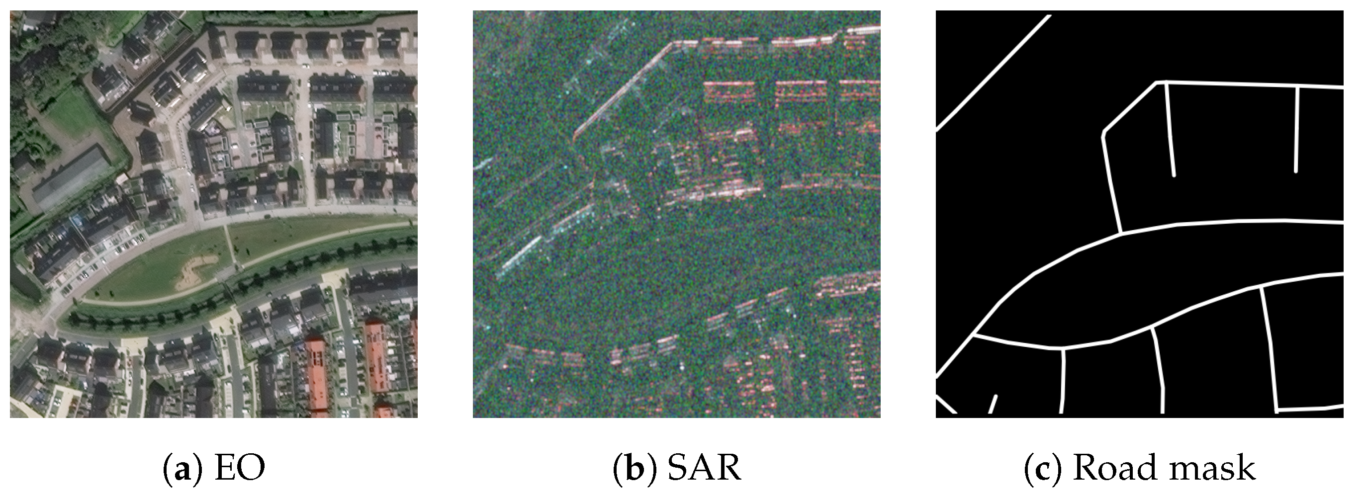
Figure 1.
(
a) An electric-optical (EO) remote sensing image. (
b) A Synthetic Aperture Radar (SAR) image of the same scene. (
c) The rasterized road mask of the scene. The EO and SAR images are from the SN6-SAROPT [
7] dataset, and the road mask is taken from OpenStreetMap.
Figure 1.
(
a) An electric-optical (EO) remote sensing image. (
b) A Synthetic Aperture Radar (SAR) image of the same scene. (
c) The rasterized road mask of the scene. The EO and SAR images are from the SN6-SAROPT [
7] dataset, and the road mask is taken from OpenStreetMap.
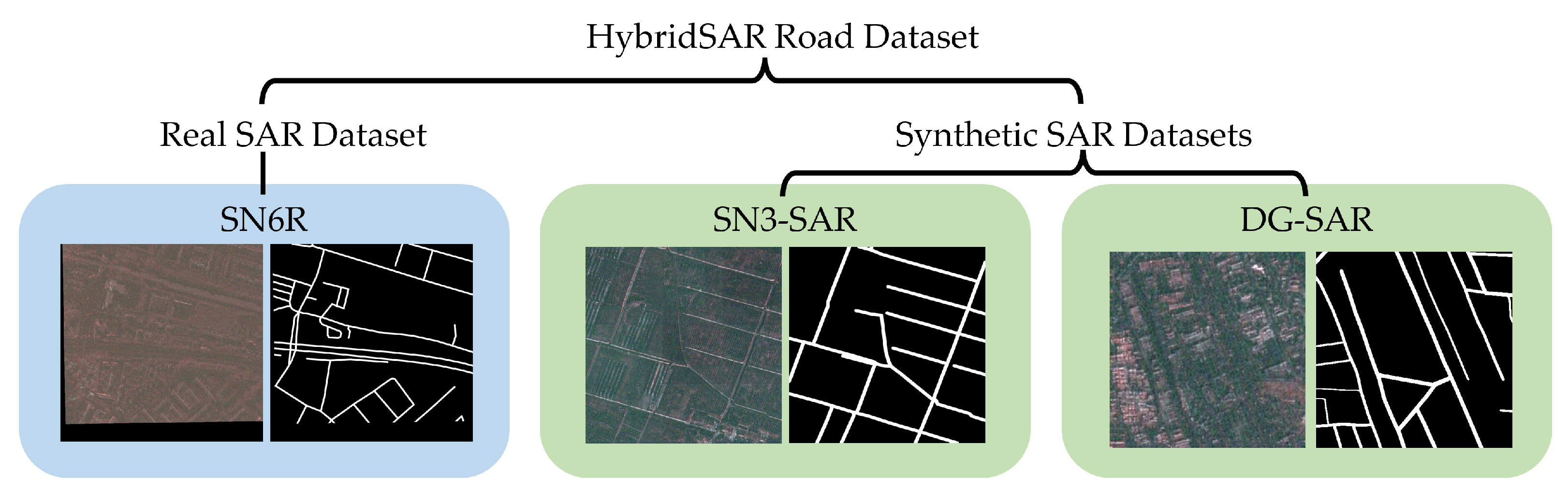
Figure 2.
The HybridSAR Road Dataset consists of one real SAR road dataset (SN6R) and two synthetic SAR road datasets (SN3-SAR and DG-SAR).
Figure 2.
The HybridSAR Road Dataset consists of one real SAR road dataset (SN6R) and two synthetic SAR road datasets (SN3-SAR and DG-SAR).
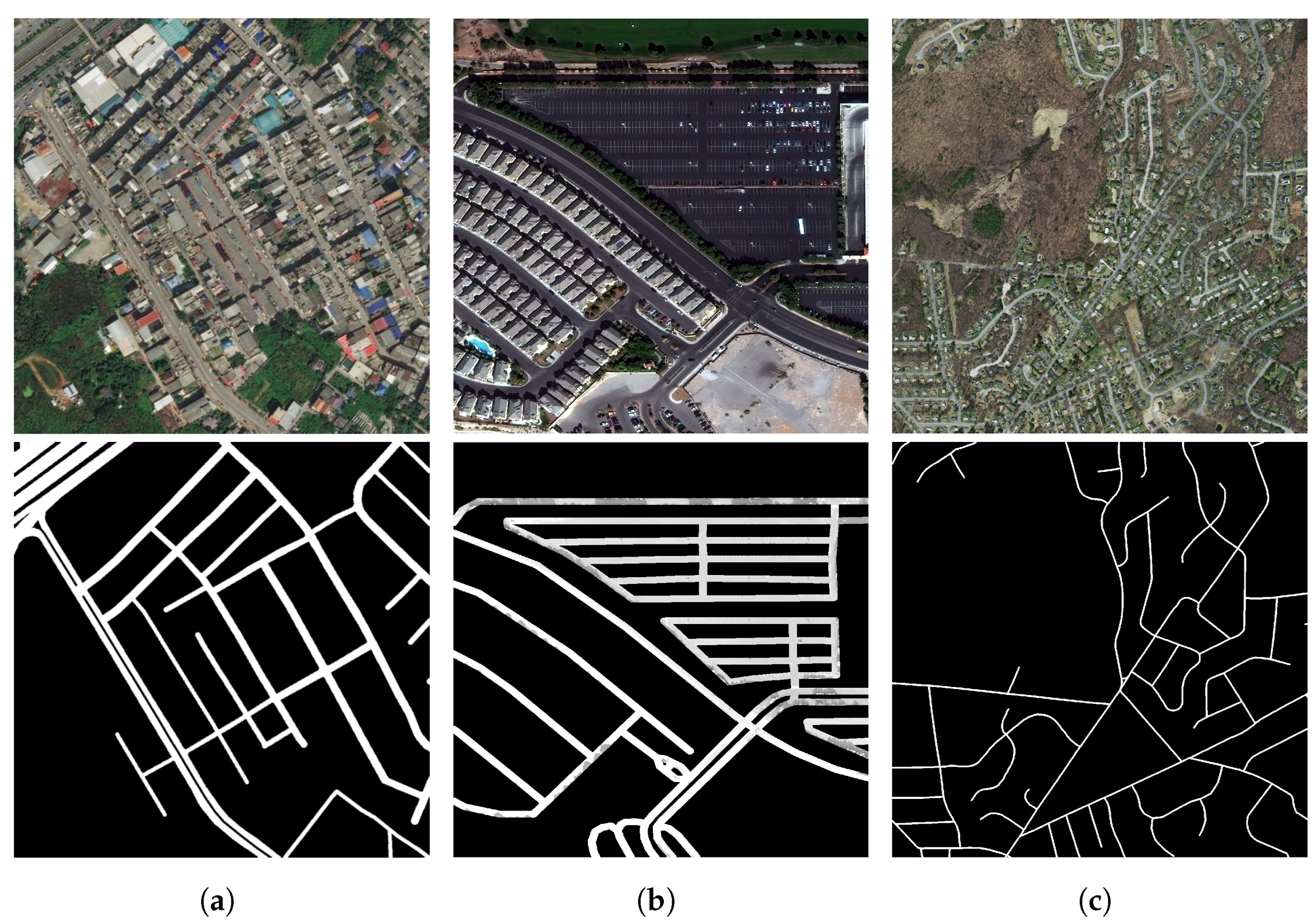
Figure 3.
Sample image and mask of the major road datasets. (a) The DeepGlobe Dataset provides labels as 512 × 512 road masks corresponding to the road surface. (b) The SpaceNet3 Road Dataset provides road centerline vectors that can be rasterized for 1300 × 1300 image tiles. (c) The Massachusetts dataset. OSM road layers are extracted and rasterized for the 1500 × 1500 image tiles.
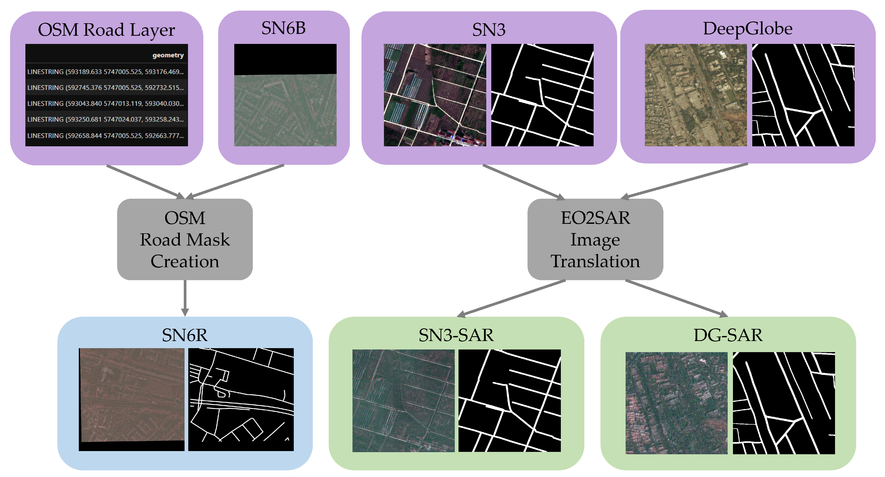
Figure 4.
Overview of the HybridSAR Road Dataset (HSRD) package creation framework. 1. Construction of the SN6R dataset by merging road layers from OpenStreetMap (OSM) with SAR image tiles from the SpaceNet 6 Building (SN6B) dataset. 2. Transformation of two optical road datasets, DeepGlobe (DG) and SpaceNet 3 (SN3), into synthetic SAR datasets (DG-SAR and SN3-SAR) through an EO2SAR translation model.
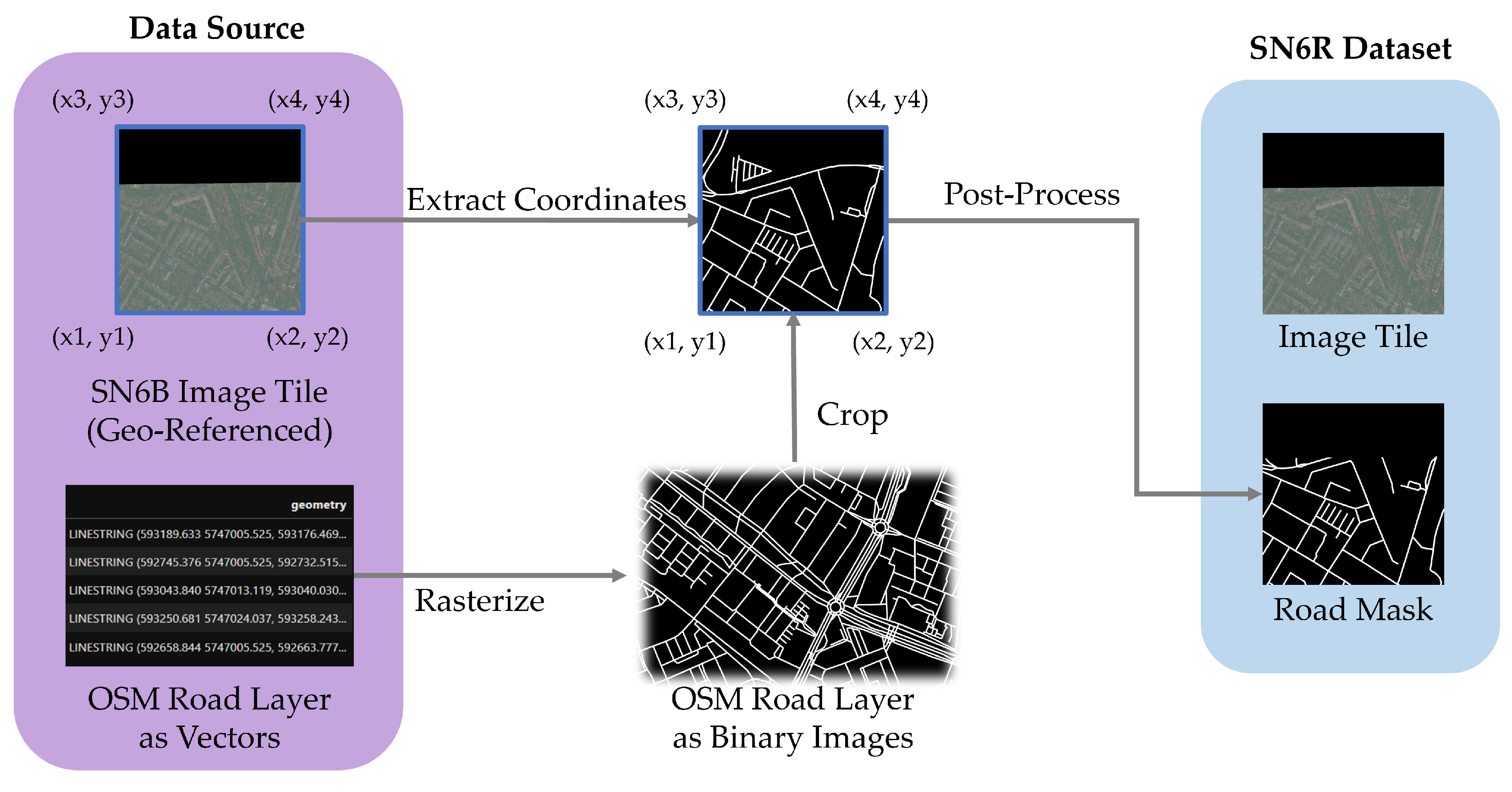
Figure 5.
Detailed process for deriving road masks from OSM for the SN6R dataset. Steps include (1) extracting coordinate information from the geo-referenced SN6B image file, (2) rasterizing OSM road vectors into binary images, (3) clipping the binary image with the coordinates, and (4) applying filtering and other post-processing methods to finalize the road mask tile.
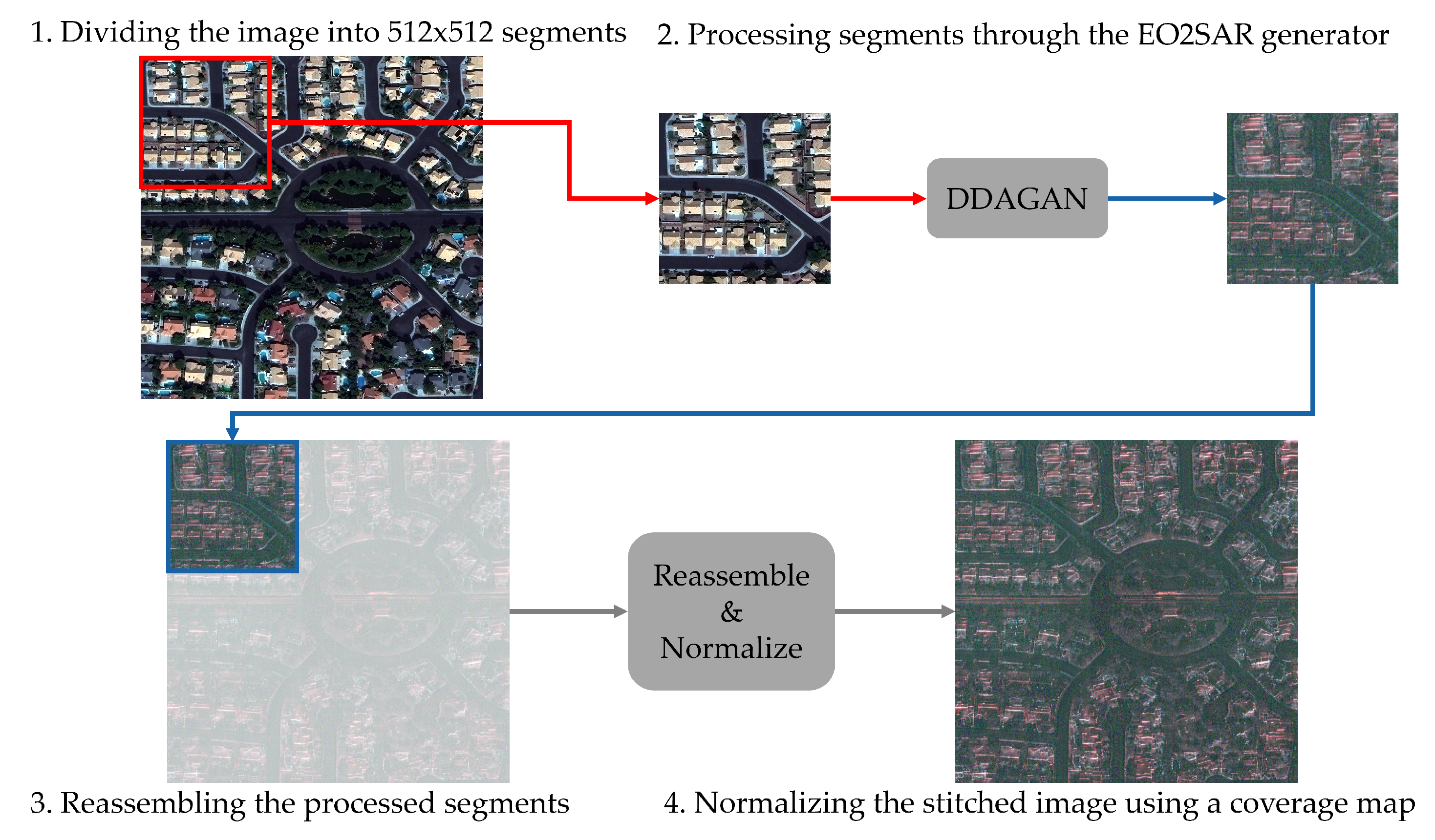
Figure 6.
The workflow of synthesizing SAR images from optical SpaceNet 3 images. (1) The 1300 × 1300 SN3 image is split into multiple 512 × 512 pieces. (2) Each piece is then fed through the EO2SAR generator of the DDAGAN model, a specialized optical-to-SAR GAN, effectively transforming the optical data into SAR-like imagery. (3) The SAR-styled pieces are stitched back together, reconstructing the full image. (4) This composite image is subsequently normalized by dividing it by a coverage map, which accounts for overlapping areas during the stitching process. (5) The final normalized SAR map, ready for further analysis or application.
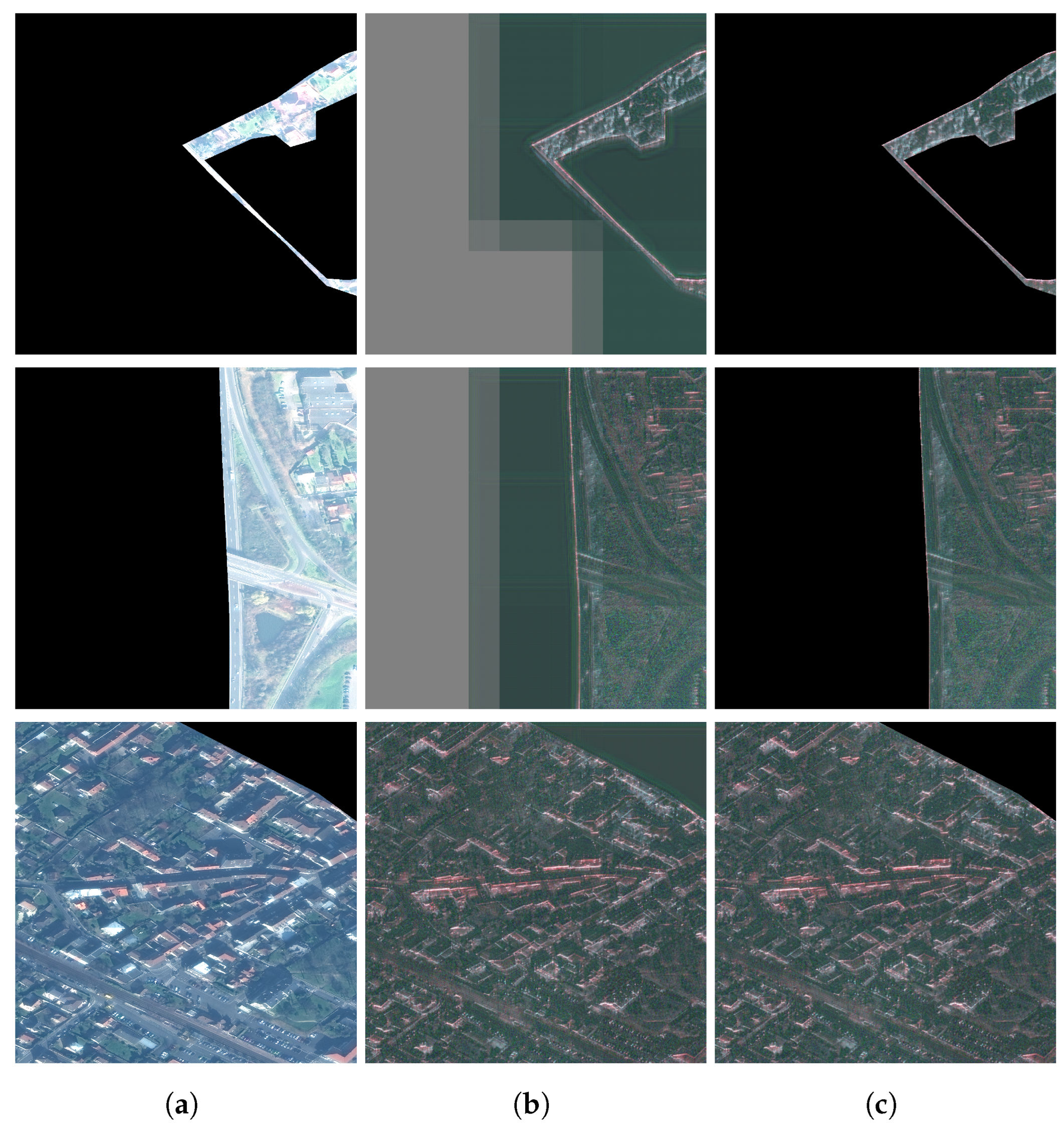
Figure 7.
Demonstration of the re-masking step of the obstructed areas in the process of createing the SN3-SAR dataset. (a) The obstructed SN3 optical images; (b) The direct output of the DDAGAN, after stitching, without re-masking; (c) The final output, after the re-masking step.
Figure 7.
Demonstration of the re-masking step of the obstructed areas in the process of createing the SN3-SAR dataset. (a) The obstructed SN3 optical images; (b) The direct output of the DDAGAN, after stitching, without re-masking; (c) The final output, after the re-masking step.
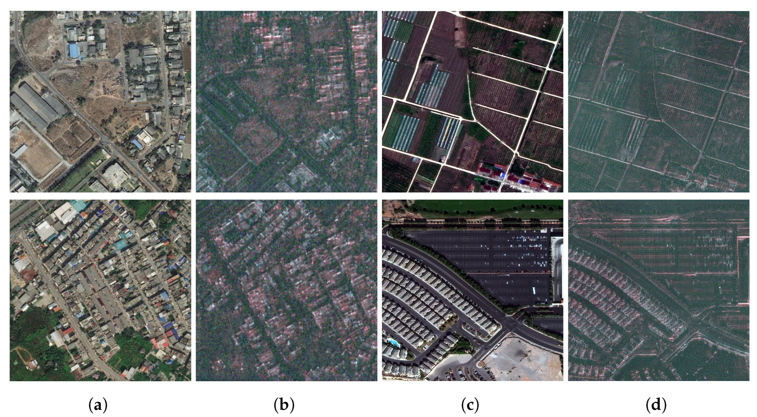
Figure 8.
Qualitative visualization results of synthetic SAR data. (a) Original DeepGlobe image tiles; (b) corresponding synthetic DG-SAR image tiles produced by DDAGAN; (c) original SpaceNet 3 image tiles; (d) corresponding synthetic SN3-SAR image tiles produced by DDAGAN.
Figure 8.
Qualitative visualization results of synthetic SAR data. (a) Original DeepGlobe image tiles; (b) corresponding synthetic DG-SAR image tiles produced by DDAGAN; (c) original SpaceNet 3 image tiles; (d) corresponding synthetic SN3-SAR image tiles produced by DDAGAN.
Figure 9.
Visualization of the SN6R training/validation/testing set’s coverage, with the map of Rotterdam as the basemap reference. Each square tile in the figure reflects the location of the corresponding SAR image tile, with white tiles in the training set, the blue tiles in the validation set, and the red tiles in the testing set. As demonstrated, there exist a large amount of overlapping tiles, which calls for a dedicated data sampling strategy. The basemap is provided by ESRI World Imagery.
Figure 10.
Segmentation results of the trained models: (a) the corresponding RGB image (for reference); (b) te SN6R SAR input image; (c) the ground truth road mask; (d) the prediction result of OnlySAR; (e) the prediction result of OpticalSAR; (f) the prediction result of HybridSAR. The red boxes highlight the differences in the segmentation results.
Table 1.
A detailed summary of the HybridSAR Road Dataset (HSRD).
Table 1.
A detailed summary of the HybridSAR Road Dataset (HSRD).
| Dataset | # of Images | Spatial Resolution | Size | Region of Interest (RoI) | SAR Image Type | Road Label Type |
|---|
| SN6R | 3401 | 0.5 m | 900 | Rotterdam | real | OSM |
| SN3-SAR | 2780 | 0.3 m | 1300 | Vegas, Paris, Shanghai, Khartoum | synthetic | manual |
| DG-SAR | 6226 | 0.5 m | 512 | Thailand | synthetic | manual |
Table 2.
Comparison of popular optical road segmentation datasets with image tiling and labeling schemes.
Table 2.
Comparison of popular optical road segmentation datasets with image tiling and labeling schemes.
| Dataset | Image Tiling Scheme | Labeling Scheme |
|---|
| Geo-Referenced | Obstructed | Road Width | Road Type |
|---|
| SpaceNet 3 | ✓ | ✓ | constant | geospatial vector data |
| DeepGlobe | × | × | varying | image mask |
| Massachusetts | ✓ | ✓ | 7 pixels | image mask |
Table 3.
Overview of the SpaceNet 3 and DeepGlobe datasets, as well as the SN6-SAROPT dataset that was used to train the DDAGAN model.
Table 3.
Overview of the SpaceNet 3 and DeepGlobe datasets, as well as the SN6-SAROPT dataset that was used to train the DDAGAN model.
| Dataset | # of Image Tiles | Size (px) | Spatial Resolution | Regions of Interest |
|---|
| SpaceNet 3 (SN3) | 2780 | 1300 | 0.3 m | Vegas, Paris, Shanghai, Khartoum |
| DeepGlobe (DG) | 6226 | 1024 | 0.5 m | Thailand |
| SN6-SAROPT | 724 × 2 | 512 | 0.5 m | Rotterdam |
Table 4.
The number of image tiles in the training, validation, and testing sets in the SN6R, SN3-SAR, and DG-SAR datasets, respectively.
Table 4.
The number of image tiles in the training, validation, and testing sets in the SN6R, SN3-SAR, and DG-SAR datasets, respectively.
| | | Training | Validation | Testing | Total |
|---|
| SN6R | 2286 | 169 | 946 | 3401 |
| DG-SAR | 4150 | 218 | 1858 | 6226 |
| SN3-SAR | 1852 | 98 | 830 | 2780 |
| sub-sets | SN3-SAR Paris | 206 | 11 | 93 | 310 |
| SN3-SAR Vegas | 661 | 35 | 293 | 989 |
| SN3-SAR Shanghai | 798 | 42 | 358 | 1198 |
| SN3-SAR Khartoum | 187 | 10 | 86 | 283 |
Table 5.
Performances of three models on road segmentation on SN6R test set. HybridSAR achieves best score in terms of IoU and F1.
Table 5.
Performances of three models on road segmentation on SN6R test set. HybridSAR achieves best score in terms of IoU and F1.
| Model | Recall | Precision | IoU | F1-Score |
|---|
| HybridSAR | 56.70 | 50.27 | 37.39 | 52.11 |
| OpticalSAR | 52.13 | 52.51 | 36.58 | 50.97 |
| OnlySAR | 59.24 | 35.72 | 28.54 | 42.88 |
Table 6.
Road segmentation results on the SN3-SAR Paris dataset.
Table 6.
Road segmentation results on the SN3-SAR Paris dataset.
| Model | Recall | Precision | IoU | F1-Score |
|---|
| OnlySAR | 58.93 | 51.27 | 36.80 | 49.35 |
| HybridSAR | 64.50 | 66.08 | 46.47 | 59.39 |
Table 7.
Road segmentation results on the DG-SAR dataset.
Table 7.
Road segmentation results on the DG-SAR dataset.
| Model | Recall | Precision | IoU | F1-Score |
|---|
| OnlySAR | 74.33 | 71.20 | 57.13 | 70.64 |
| HybridSAR | 77.34 | 68.75 | 57.42 | 71.12 |
Table 8.
Performance comparison of the XDXD model, which was designed for building segmentation, with the HybridSAR model used in our study.
Table 8.
Performance comparison of the XDXD model, which was designed for building segmentation, with the HybridSAR model used in our study.
| Model | Recall | Precision | IoU | F1-Score |
|---|
| XDXD | 92.50 | 7.11 | 7.06 | 13.03 |
| HybridSAR | 56.70 | 50.27 | 37.39 | 52.11 |


