Enhancing the Resolution of Satellite Ocean Data Using Discretized Satellite Gridding Neural Networks

Abstract

Ocean satellite data are often impeded by intrinsic limitations in resolution and accuracy. However, conventional data reconstruction approaches encounter substantial challenges when facing the nonlinear oceanic system and high-resolution fusion of variables. This research presents a Discrete Satellite Gridding Neural Network (DSGNN), a new machine learning method that processes satellite data within a discrete grid framework. By transforming the positional information of grid elements into a standardized vector format, the DSGNN significantly elevates the accuracy and resolution of data fusion through a neural network model. This method’s innovative aspect lies in its discretization and fusion technique, which not only enhances the spatial resolution of oceanic data but also, through the integration of multi-element datasets, better reflects the true physical state of the ocean. A comprehensive analysis of the reconstructed datasets indicates the DSGNN’s consistency and reliability across different seasons and oceanic regions, especially in its adept handling of complex nonlinear interactions and small-scale oceanic features. The DSGNN method has demonstrated exceptional competence in reconstructing global ocean datasets, maintaining small error variance, and achieving high congruence with in situ observations, which is almost equivalent to 1/12° hybrid coordinate ocean model (HYCOM) data. This study offers a novel and potent strategy for the high-resolution reconstruction and fusion of ocean satellite datasets.

1. Introduction

Satellite remote sensing technology has become an indispensable and increasingly important means of marine environmental monitoring. It has the characteristics of a large scale, wide coverage, and strong continuity, which can make up for the shortcomings of traditional monitoring, and it is very suitable for the long-term continuous monitoring of the ocean environment. Therefore, it has become an important method in global marine research in recent years [1,2,3,4]. However, satellite ocean data also has some inherent defects; for example, the remote sensing image and its quantitative inversion products are significantly affected by clouds and precipitation. Most optical satellites equipped with ocean observation sensors are in the polar orbit, the coverage of a single sensor is limited, and the gap between the probe orbits will affect the spatial resolution [5,6]. Therefore, using relevant data reconstruction methods to effectively reconstruct satellite data is of great significance to improve the application value of remote sensing quantitative observation data. Meanwhile, current research has put forward higher requirements for the accuracy of satellite ocean products, such as marine submesoscale research [7]. Therefore, it is necessary to improve the spatial resolution of satellite data in order to obtain local detail features accurately.

The traditional satellite data reconstruction method is mainly interpolation filling, which involves estimating the missing data according to the values of surrounding pixels, such as optimal and Kriging interpolation for the reconstruction of the global sea surface temperature (SST) [8,9]. Later, a method based on the empirical orthogonal function (EOF) has been used to reconstruct satellite data. It can reconstruct large areas of missing data and has been applied to the SST, sea surface chlorophyll a, sea level anomaly (SLA), and other datasets [10,11]. With the development of deep learning technology, more and more researchers are beginning to use deep learning models, such as convolutional neural networks (CNNs) and recurrent neural networks (RNNs), to carry out the spatial reconstruction of satellite data and obtain reliable results in terms of accuracy and computational efficiency. These methods can effectively capture the complex spatial distribution and time dependence of the data, making them a new solution for data reconstruction [12,13,14,15]. In addition, with the reconstruction process, we can further use the “spatial downscaling” method to improve the spatial resolution of the satellite data. Downscaling can improve the resolution of the original data or deduce local detail features from a large range of regional features. At present, there are two kinds of downscaling methods: dynamic and statistical downscaling [16]. There are similarities between the downscaling technique and image super-resolution, such as random forest (RF) and support vector machine (SVM), which also have good results in downscaling [17,18].

Furthermore, researchers noticed that satellite data fusion (the synthesis of multi-source satellite data in the same area) can produce more accurate, complete, and reliable estimations and judgments than a single information source [19,20,21]. Traditional data fusion methods include algebraic methods, image regression, principal component transformation, wavelet transform, Bayesian estimation, Dempster–Shafer inference methods, and other technologies [22]. In the multi-source data fusion task of satellites, the application of machine learning technology has made remarkable progress [23,24,25]. The main advantage of machine learning is that it can automatically and effectively identify complex relationships and extract features from different types of raw data. It can learn complex nonlinear relationships between image blocks through multi-layer nonlinear mapping and extract advanced features and patterns in satellite data [26]. These methods do not require a preset model and can learn end-to-end fusion mapping, thus effectively improving the quality of fusion. The design of the network structure directly affects the quality of the results. Further research still needs to show how to design a more reasonable network structure, deal with the spatial–temporal discontinuity of satellite data, and improve the accuracy of satellite datasets [25,27].

This study proposes a new method called the Discrete Satellite Gridding Neural Network (DSGNN) for the high-resolution reconstruction and fusion of satellite ocean data. The DSGNN processes satellite data through a unified discrete grid, scatters the position information of different elements of different grids into a standardized special position vector, and uses a neural network model for data fusion and prediction. Compared with traditional methods, the DSGNN has obvious advantages in satellite data fusion tasks. We further compare it with a high-resolution ocean numerical model (HYCOM), and the results show that the DSGNN performs almost as well. The above results fully prove the huge application potential of deep learning technology in satellite ocean data fusion and reconstruction in the future.

2. Data and Methods

2.1. Data: SST/SSS/SLA/ADT

We combine four types of datasets: sea surface temperature (SST), sea surface salinity (SSS), sea level anomaly (SLA), and absolute dynamic altitude (ADT). They are four key satellite datasets that describe the state of the ocean, and they are closely linked and, together, form a comprehensive picture of the physical state of the ocean [28].

The SST and SSS are the main factors that determine seawater density and ocean stratification, and their changes directly affect the ocean’s thermohaline circulation [29]. An increase in the SST usually results in an increase in seawater volume, which is reflected by a rise in sea level in SLA; conversely, a decrease in the SST leads to a decrease in sea level. Changes in the SSS also affect the sea level because changes in salinity change the density and volume of seawater, which, in turn, affects SLA. Both SLA and the ADT describe sea level changes, but SLA reflects more short-term and seasonal changes, while the ADT provides a perspective of long-term changes. The ADT takes into account the influence of dynamic processes within the ocean and provides a more comprehensive perspective of sea level changes. It is related to changes in both the SST and SSS because changes in these parameters will affect the density of seawater and the dynamics of sea level [30].

2.1.1. Data: SST Data of AVHRR

The Optimum Interpolation Sea Surface Temperature (OISST) refers to a global analysis product ranging from a weekly 1° grid to the latest daily 1/4° grid. The OISST is a spatially gridded product created by interpolating and extrapolating data that combine ocean temperature observations from an Advanced Very High Resolution Radiometer (AVHRR) and in situ platforms such as ships and buoys (https://www.noaa.gov/) (accessed on 14 August 2024) [31]. The input data of the OISST are irregularly distributed in space and must first be placed on a regular grid, and then the optimal interpolation method is applied to fill the positions of missing values [32]. The method involves bias correction of satellite data before interpolation. The OISST is used in weather forecasting, climate research, modeling, fisheries ecology, oceanography, and as a reference field for other satellite algorithms.

2.1.2. Data: SSS Data of SMOS

SSS data from the Soil Moisture and Ocean Salinity (SMOS) satellite provides the salinity of the ocean surface (https://marine.copernicus.eu/) (accessed on 14 August 2024) [33]. The unit of SSS is Practical Salinity Unit (PSU), which represents the amount of salt dissolved in seawater per kilogram (roughly equivalent to one liter of volume). The retrieval of the SSS is based on the maximum likelihood Bayesian method, and the SSS is obtained by comparing the brightness temperature, Tbimeas, measured by SMOS at different incident angles θ_i with the brightness temperature modeled by T_b. These measured data need to be fit into a direct model to find the best solution for the parameters. Its spatial resolution is also about 1/4° [34].

2.1.3. Data: SLA Data of CMEMS

The SLA data provided by Archiving, Validation and Interpretation of Satellite Oceanographic (AVISO) data is a result of the fusion of altimeter measurements from various satellite missions, including T/P (TOPEX/Poseidon), Jason-1, Jason-2, Jason-3, ERS, and ENVISAT, among others. This fusion process ensures the continuity and consistency of the dataset over an extended period (https://www.aviso.altimetry.fr/) (accessed on 14 August 2024) [35]. With a spatial resolution of approximately 1/4°, the SLA dataset is able to characterize small-scale and large-scale changes in the ocean surface, which may be caused by wind, waves, tides, temperature changes, and circulation patterns. The SLA is critical to understanding ocean flow field and circulation patterns and improving the predictability of the ocean and climate change [36].

2.1.4. Data: ADT Data of CMEMS

The ADT is another dataset provided by AVISO (https://www.aviso.altimetry.fr/) (accessed on 14 August 2024). It is similar to SLA, but the ADT is calculated relative to the geoid. The ADT dataset provides the absolute dynamic topography of the ocean surface height, calculated by subtracting mean sea surface (MSS) and mean dynamic topography (MDT) from the sea surface height (SSH), which is directly measured using satellite altimeters. The ADT represents the sea surface height above the geoid, taking into account the static and dynamic contributions to sea level variations. It combines information from altimeter measurements with geophysical corrections and models to provide a comprehensive view of ocean topography. Its spatial resolution is also 1/4°. The ADT is also useful for oceanographic and climate studies because it provides a detailed view of the ocean surface height, helping us understand ocean circulation and sea level changes [37].

2.1.5. Data: EN4.2.2

The EN4.2.2 is a high-quality ocean temperature and salinity profile dataset that combines observations from multiple sources, including ships, buoys, Argo buoys, and satellite observations. The dataset is carefully quality-controlled and bias-corrected, providing a detailed view of the state of the ocean from the surface to the deep ocean. The EN4.2.2 dataset is a scatter dataset of ocean temperature and salinity (T/S) profiles provided by the Met Office Hadley Centre (MOHC) (https://www.metoffice.gov.uk) (accessed on 14 August 2024) [38]. In this study, these data are not used as training data, but as benchmark values to determine the quality of satellite data interpolation under different models.

2.1.6. Data: HYCOM

The HYCOM is a data-assimilated hybrid isobaric sigma-pressure (generalized) coordinate ocean model, which is developed jointly by multiple agencies, including the National Ocean Partnership Program (NOPP), as a part of the U.S. Global Ocean Data Assimilation Experiment (GODAE). The dataset has a spatial resolution of approximately 1/12° (approximately 8.5 km) and provides temperature and salinity information from the sea surface to the deep sea. The depth layer ranges from 0 to 5000 m (https://www.hycom.org/hycom/) (accessed on 14 August 2024) [39,40]. The HYCOM is designed to effectively simulate ocean flows in the upper layers, thermocline, and deep ocean. It overcomes the limitations of traditional models by employing a mixed coordinate system, allowing for a more accurate depiction of oceanic processes. In this study, HYCOM is used as valuable comparative data to demonstrate the superiority of our satellite approach. The HYCOM is only used for making a comparison, and not for training. The comparison of all the above data used in this study is shown below (

Table 1. The data used in this study.

Data Name	Data Source	Resolution	Description
SST	AVHRR	1/4°	Satellite remote sensing
SSS	SMOS	1/4°	Satellite remote sensing
SLA	AVISO	1/4°	Satellite remote sensing
ADT	AVISO	1/4°	Satellite remote sensing
EN 4.2.2	MOHC	scatter	In situ observation
HYCOM	GODAE	1/12°	Ocean model data

).

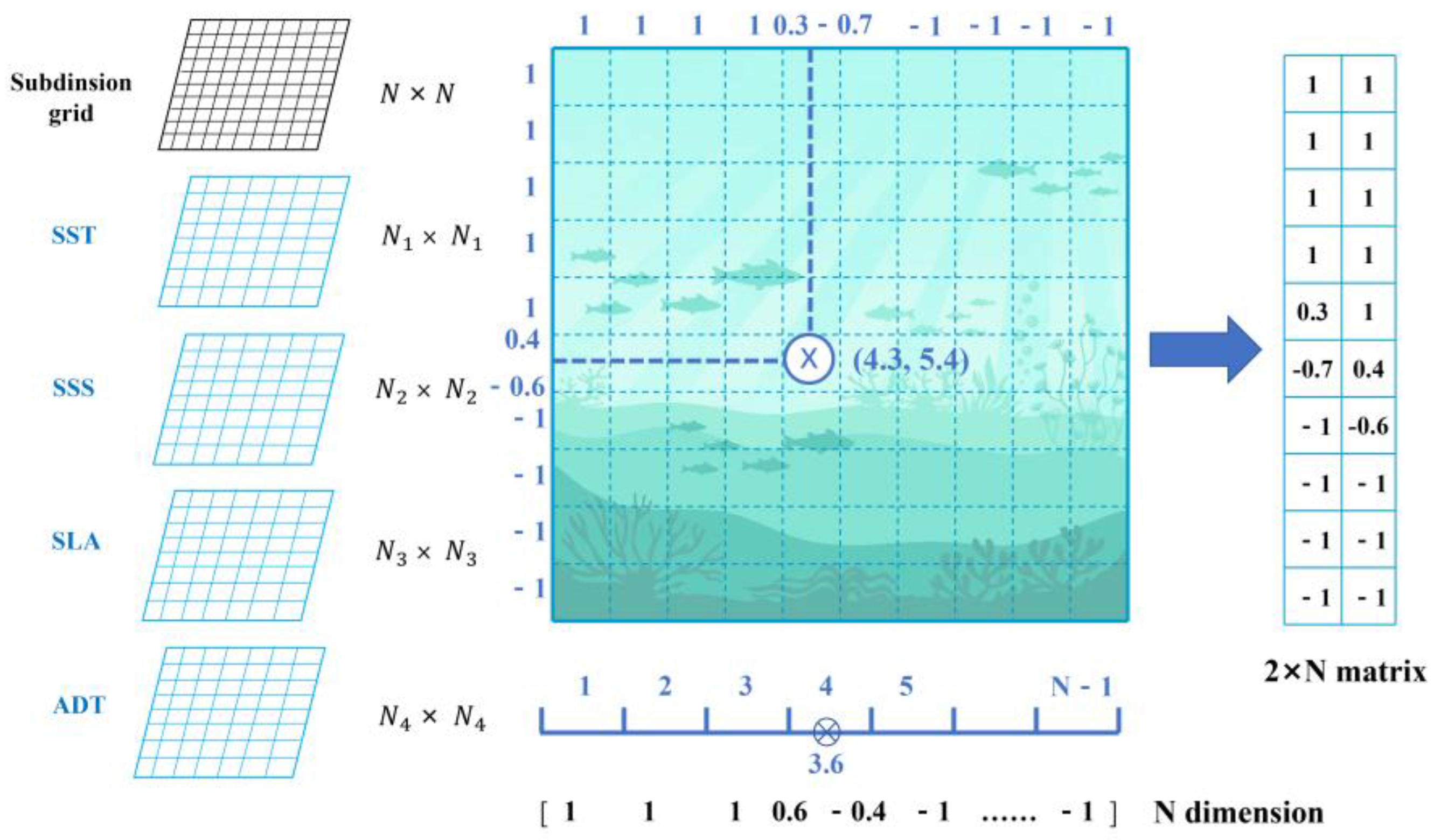
2.2. Discretization Method

Due to the huge amount of continuous data in the training set, we want to preprocess them effectively before inputting them in the model to speed up the data modeling process and improve the accuracy of the model. Among the available methods, discretization is a common and effective data preprocessing method [40,41]. In this study, we propose a new method called spatial discretization, where the input latitude and longitude data are discretized into a specialized vector. This mathematical technique is relatively inspired by hash encoding and isometric discretization [42,43].

This project changes any two-dimensional coordinate within the grid into a series of boundary discretized values by using the two steps. Firstly, in a two-dimensional coordinate point X (λ, ϕ), where λ and ϕ represent the longitude and latitude values, the following formula can be used to determine the latitude and longitude grid:

$$i=\lfloor {\displaystyle \frac{\lambda -{\lambda }_{\min }}{\mathrm{\Delta }\lambda }}\rfloor +1,j=\lfloor {\displaystyle \frac{\varphi -{\varphi }_{\min }}{\mathrm{\Delta }\varphi }}\rfloor +1$$

(1)

⌊⋅⌋ represents the downward rounding operation, Δλ and Δϕ are the spacing of the grid in the longitude and latitude directions, and λ_min and ϕ_min refer to the minimum values of the longitude and latitude range. In this way, we can map any geospatial coordinate point to the corresponding discrete grid position, thereby converting it into a series of discretized values. A new vector space method is introduced to maintain the information of the original coordinates within the grid:

$$f\left(\lambda \right)=\left\{\begin{array}{c}-1,if\lambda <{\lambda }_i\\ 1,if\lambda >{\lambda }_i+\Delta \lambda \\ \lambda -{\lambda }_i,if{\lambda }_i\le \lambda \le {\lambda }_i+\Delta \lambda \end{array}\right.$$

(2)

$$f\left(\varphi \right)=\left\{\begin{array}{c}-1,if\varphi <{\varphi }_j\\ 1,if\varphi >{\varphi }_j+\Delta \varphi \\ \varphi -{\varphi }_j,if{\varphi }_j\le \varnothing \le {\varphi }_j+\Delta \varphi \end{array}\right.$$

(3)

This results in a normalized vector component that ranges from −1.0 to 1.0, thereby encapsulating the original coordinate’s spatial context within its grid cell. Secondly, by dividing a (N−1) × (N−1) latitude and longitude area into a 1° × 1° grid, each coordinate is presented as an N-dimensional vector. For instance, when N = 10 and the longitude is 4.6, the vector is expressed as [1, 1, 1, 1, 0.6, −0.4, −1, −1, −1, −1]. The latitude is processed similarly, leading to a 2 × N matrix that represents the spatial coordinates for each data point. Then, SST, SSS, SLA, and ADT data can be unified under the integrated resolution (as shown in Figure 1). They can simplify the model and reduce the risk of overfitting as well as permit the use of a smaller network without sacrificing quality, thus significantly reducing the number of floating points [41,44,45,46]. The specific program design is shown in Appendix A.

2.3. Neural Network Construction

2.3.1. Network Architecture

A deep neural network model was developed to improve the prediction accuracy of the temperature (T) and salinity (S) in four-dimensional ocean data, including the longitude (λ), latitude (ϕ), depth (z), and time (t). This model includes connected layers (FCL) and Leaky Rectified Linear Unit (ReLU) layers to deal with preprocessed spatiotemporal discretized data. The input layer receives the discretized data D (λ, ϕ, z, t) and FCL layers, obtaining the following: Rⁿ→R^m and the Leaky ReLU activation function f(x) = max (0.01x, x). This study performs high-resolution missions for SST/SSS/ADT/SLA, so the input data has a low resolution, and the output is high-resolution satellite data (Figure 2). Oceanographic data have significant spatio-temporal characteristics, that is, there are correlations in both time and space. Deep learning models can capture this spatio-temporal correlation and achieve the effective fusion of multi-source data.

Although they represent different physical quantities, these datasets can be used as different inputs to the fully connected layer. In the model, these datasets are usually preprocessed to be unified into the same spatial resolution and format. By carrying this out, even though the datasets have different physical meanings, they become numerically compatible and can be input into the same neural network for processing. One of the primary functions of a fully connected layer is to achieve the fusion and combination of input features. By using the SST, SSS, ADT, and SLA as different inputs to the fully connected layer, the model can learn the nonlinear relationships between these variables and generate more expressive feature representations. These representations can help the model make more accurate predictions or classifications because they consider the combined effects of multiple variables.

2.3.2. Weight Decay

Weight decay is also called L2 regularization; it is a common technique for parameterizing machine learning models, and it achieves the effect of regularization through adding a regularization term to the loss function. That is proportional to the L2 norm, like the sum of squares of the model’s weight vector. In this way, weight decay can limit the size of the model’s weights and mitigate the overfitting risks. The model’s loss function is L, the modified loss function is L′, and the weight decay can be formulated as follows:

$$L\prime =L+{\displaystyle \frac{\lambda }{2}}||w|{|}^2$$

(4)

L is the original loss function, λ is the regularization coefficient, and $||w|{|}^2$ stands for the L2 norm of the model’s weight vector. When the input dimension is high, the complexity of the model increases rapidly with the degree. Given d variables, the number of monomials with degree D can be expressed as follows: $\left(\begin{array}{c}d+D-1\\ D\end{array}\right)$. Accordingly, a more granular tool is needed to simplify the function. For linear regression models, the loss can be formulated as follows:

$$L={\displaystyle \frac{1}{n}}{{\displaystyle {\sum }_{i=1}^n(y_i-w^T{x}_i-b)}}^2$$

(5)

where x_i represents the features, y_i represents the labels, w is the weight, and b represents the bias parameters. Then, the loss function can be expressed as follows:

$$L\prime =L+{\displaystyle \frac{\lambda }{2n}}||w|{|}^2$$

(6)

where n refers to the number of data points, and it guarantees that the regularization term’s magnitude is independent of the sample size. The modified formula can be presented as follows:

$$w\leftarrow w-\alpha ({\displaystyle \frac{\mathsf{\partial }L}{\mathsf{\partial }w}}+{\lambda }_w)$$

(7)

where α is the learning rate, λ refers to the weight decay coefficient, and ${\displaystyle \frac{\mathsf{\partial }L}{\mathsf{\partial }w}}$ is the partial derivative of the loss function L with respect to the weight w. This modified rule considers the factor of reducing training error and takes the magnitude of w into consideration to reduce the model complexity. In practical applications for high-dimensional and noisy oceanographic data, weight decay can be an effective technique to make sure that deep learning models can provide reliable predictions. When dealing with continuous, high-dimensional datasets like ocean satellite data, L2 regularization is particularly effective. Firstly, L2 regularization imposes a penalty on the square of the weights, which encourages the weights to be as close to zero as possible but not exactly zero. This is very important for models that need to capture subtle variations in the dataset. For ocean satellite data, many physical processes are characterized by small but continuous changes, and the smoothing effect of L2 regularization can help the model better capture these details. Secondly, L2 regularization is commonly used in deep learning models because it can provide more stable convergence during optimization, especially when dealing with complex nonlinear models. This is particularly important for the DSGNN, which needs to handle a large amount of high-dimensional data, as stable convergence can improve training efficiency and prevent overfitting.

2.3.3. Design of Loss Function and Data Testing Criteria

An effective loss function is essential in optimizing model parameters to promote prediction accuracy. If a model’s predicted output is $y_{pred}$, and the corresponding true label is $y_{true}$, when it comes to the multi-label case, the loss function can be designed as follows:

$$L(y_{pred},y_{true})={\displaystyle \frac{1}{N}}{\displaystyle {\sum }_{i=1}^N{L}_i(y_{pre{d}_i},y_{tru{e}_i})}$$

(8)

N represents the number of labels, and L_i stands for the loss calculation function for the ith label. For multi-label learning tasks, when a data point has two labels, the loss L_i is the average of the losses for the two labels. When there is only one label, the loss for that label can be used directly.

When it comes to the entire training set, the total loss $L_{total}$ is the average of the losses for all data points:

$$L_{total}={\displaystyle \frac{1}{M}}{\displaystyle {\sum }_{j=1}^{M}L(y_{pred}^{(j)},y_{true}^{(j)})}$$

(9)

M is the total number of data points. By minimizing the total loss $L_{total}$, the model’s parameters can be updated through using the backward propagation algorithm. Using the Adam optimizer can be a solution. Through changing the learning rate, the Adam optimizer can achieve fast and stable convergence in deep learning.

3. Results

3.1. Effectiveness of Satellite Global Data Reconstruction

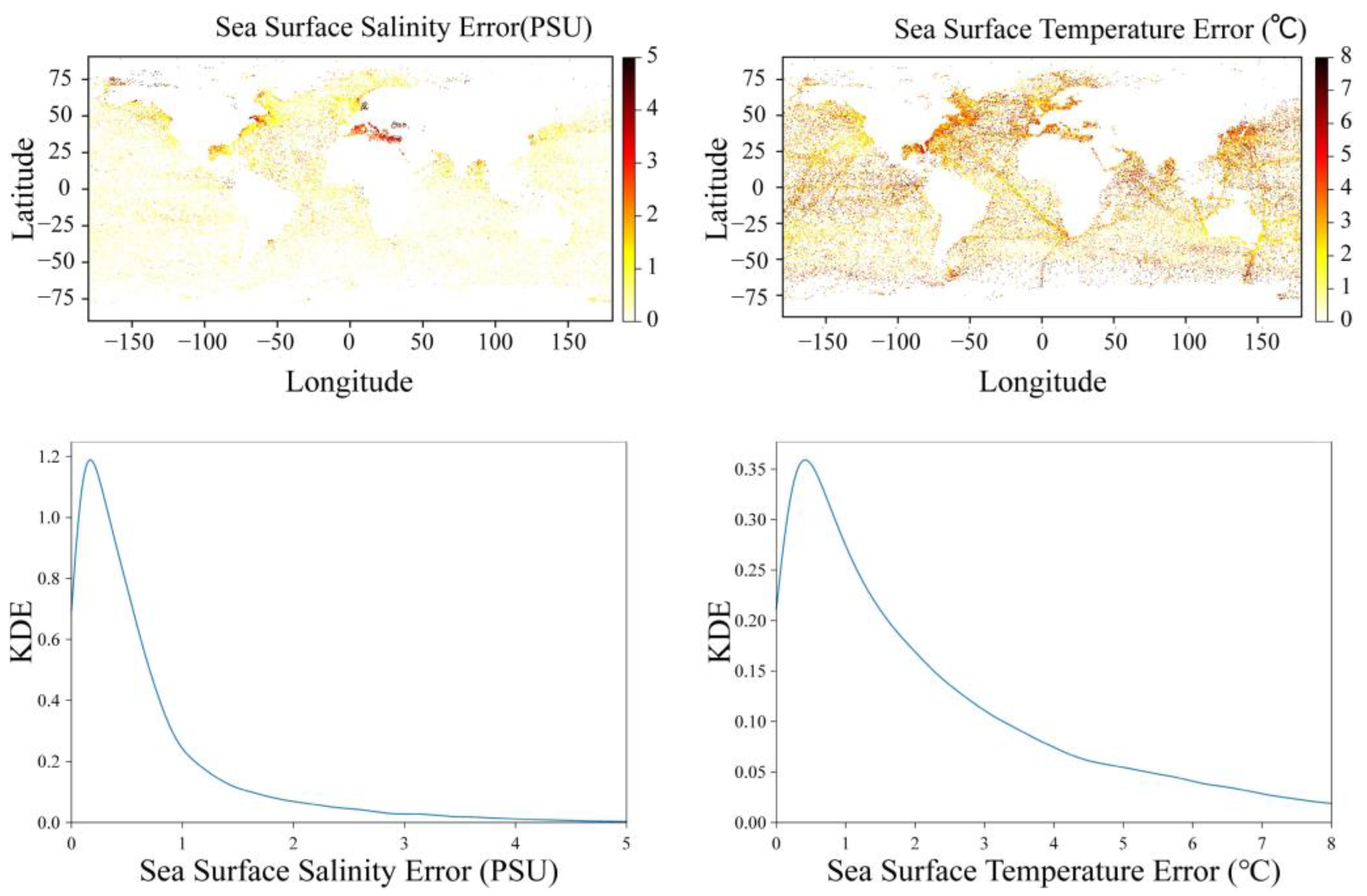
We chose a ratio of 99:1 for the selection of the training set samples with respect to the testing set. Based on the above deep learning model, we fused and reconstructed four kinds of 1/4° satellite data, and the resolution of the output new datasets were improved to 1/12°. Figure 3 shows the spatial distribution characteristics for the SST, SSS, ADT, and SLA with latitude and longitude, and this trend effect is generally consistent with previous knowledge. SLA is the deviation of sea level from the long-term average, which can be positive or negative. It has removed the effect of long-term mean sea level height and, therefore, can represent the dynamic height caused by mesoscale processes in the ocean. In Figure 3b, we can see that the active regions of global mesoscale vorticity mainly include the North Atlantic Ocean, the Northwest Pacific Ocean, and other seas such as the Indian Ocean and the Southern Ocean. This is in good agreement with the research conclusions on the characteristics of mesoscale vortices in physical oceanography.

The SSS is higher in subtropical areas with strong evaporation, such as the subtropical convergence zone of the Atlantic and Pacific Oceans. In areas with heavy precipitation, such as near the equator and some coastal areas, the SSS will be relatively low, as shown in Figure 3c. Also, salinity is affected by factors such as river input and melting sea ice, resulting in uneven distribution along the longitude and latitude. Figure 3d shows a vivid rendering effect of SST reconstruction. The SST is highest near the equator and gradually decreases toward the poles, showing a latitudinal gradient. At the same latitude, the SST may vary significantly due to the influence of ocean currents, such as warm currents and cold currents. Moreover, the SST also varies at different longitudes and is affected by ocean circulation and local heating/cooling processes. Overall, the interpolation results are consistent with the basic physical laws of the ocean and can well represent the spatial and temporal distribution characteristics of the SST, SSS, ADT, and SLA.

3.2. Error Analysis

Figure 4 shows the error scatters of the ADT, SLA, SSS, and SST in four different seasons of the year, including fourteen years (from 2010 to 2023) of averaged values from 1 January, 1 April, 1 July, and 1 October, respectively. We take the data from the EN4.2.2 dataset as the true values and then interpolate the reconstructed datasets into the corresponding grid points to calculate the error.

In the figures in the first column, it can be seen that there is little difference between the four seasons, meaning that the ADT loss does not change over different seasons. Similar results can be found when comparing seasonal error changes in the SLA. A remarkable feature of the two is that the maximum loss scatters are basically concentrated in the mid-latitude regions. The SSS error is the smallest among the four reconstructed data. On one hand, this may be because the global SSS fluctuation is relatively small; on the other hand, it also indicates the high accuracy of the reconstructed data. Additionally, this Figures in the fourth column compare the SST loss in four seasons, and it seems that the error is much more significant in January (winter) and July (summer) than in the other months. Furthermore, there are also significant differences in the regional distribution of SST errors in different seasons. For example, the error is larger in the North Atlantic region in July, while in January, the error is obvious in the mid-high latitude Pacific region. Based on Figure 4, it can be suggested that there are no significant error differences in different seasons for the ADT, SLA, and SSS. Although the seasonal difference in SST error distribution is more obvious than others, it is also within a reasonable range.

We also calculate the global monthly averaged Root Mean Square Error (RMSE). Figure 5 demonstrates the RMSE curve for different months regarding the ADT, SLA, SSS, and SST. The four datasets have maintained almost the same RMSE for over a year, with basically no changes in the curves regarding the ADT, SLA, and SSS. Corresponding to the spatial distribution diagram above, the error of SST has relatively significant seasonal fluctuations, with the RMSE being larger in July and December, while the smallest values are in March and October (Figure 5d). In general, the high-resolution data reconstructed by the DSGNN model has good stability and accuracy in the time and space dimension, which also proves the excellent performance of the model. As for the seasonal variation in the errors, we note that the error scatters are mainly distributed in the regions where mesoscale vortices and ocean fronts are active, such as the Kuroshio and the extended body regions [44]. These regions have strong seasonal changes in the sea state and are susceptible to air–sea interactions. This may be an important cause of seasonal errors.

In addition, the kernel density estimation (KDE) is a common probability density plot approach that can be used to visualize frequency data in the field of geoscience and ecological studies [47]. Through KDE curves, we can intuitively observe the distribution patterns of the multi-modal structures, skewness, and potential anomalies. In this paper, we mainly make use of the anomaly detection function of KDE, that is, by estimating the probability density of the data, we can identify samples in low-density regions as outliers. The robustness and accuracy of the model can be evaluated according to the results. When comparing the KDE curve of the ADT, SLA, SSS, and SST, it can be noticed that the data distribution of the ADT, SLA, SSS, and SST has a small error as the majority of datasets are distributed in a small range, which can be reflected in the peaks of the datasets, as shown in Figure 6.

3.3. Regional Analysis

Figure 4 shows that there are still certain differences in data quality in different regions. So, we chose five representative regions (North Atlantic, South Atlantic, Indian, North Pacific, and South Pacific Oceans) of the global ocean and calculate the loss curves for different months and years (shown in Figure 7). In terms of the loss of ADT in different months, it can be seen that the North Pacific and North Atlantic Oceans have much bigger errors than the South Atlantic Ocean, Indian Ocean, and South Pacific Ocean. For the similar error loss of the North Pacific and North Atlantic Oceans, it is clear that in July, August, and September, the North Pacific Ocean demonstrates greater error loss than the North Atlantic Ocean. However, in October, the North Atlantic and North Pacific Oceans share the same error loss. By contrast, when it comes to the ADT in different years, it can be seen that from 2010 to 2020, the North Pacific and North Atlantic Oceans had bigger error losses than the other ocean regions. Similar results show the loss of SLA in different months and different years.

There are little fluctuations in the loss of SSS in different months and years, meaning that the loss for different oceans is not significant in different months and years. For the loss of SST in different months and different years, it can be seen that different oceans have little difference in December, January, and February. However, from March to October, more apparent losses exist for different oceans. Specifically, the North Pacific Ocean has more errors in May, but the North Atlantic Ocean has more errors in June, July, August, September, October, and November. Regarding different years, generally, the North Atlantic and North Pacific Oceans have more loss than the other oceans. From a long-term perspective, the interpolation effect in the South Pacific Ocean is better, followed by the South Atlantic, Indian, North Atlantic, and North Pacific Oceans, which shows that the datasets in this area need further research to determine their quality.

The source of error is mainly due to two aspects. The first is because the data used as the training set itself have certain errors. The SST, as an example, essentially comprises reanalysis data with optimal interpolation, and there are some errors in the measured data. Secondly, the deep learning model used in this paper is still a relatively simple fully connected neural network, which has undergone a preliminary exploration. Correspondingly, if we want to reduce the error, we can start from two aspects. Taking the SST as an example, we can first carry out satellite and in situ data fusion for single elements. We can use daily data from MODIS onboard the AQUA satellite and AMSR2 onboard the Global Change Observation Mission 1st-Water (GCOM-W1) satellite at the same equatorial crossing local time, as well as the OISST data [48,49]. For deep learning models, we can choose more complex and effective convolutional neural networks or physical information neural networks to improve the effect of model training.

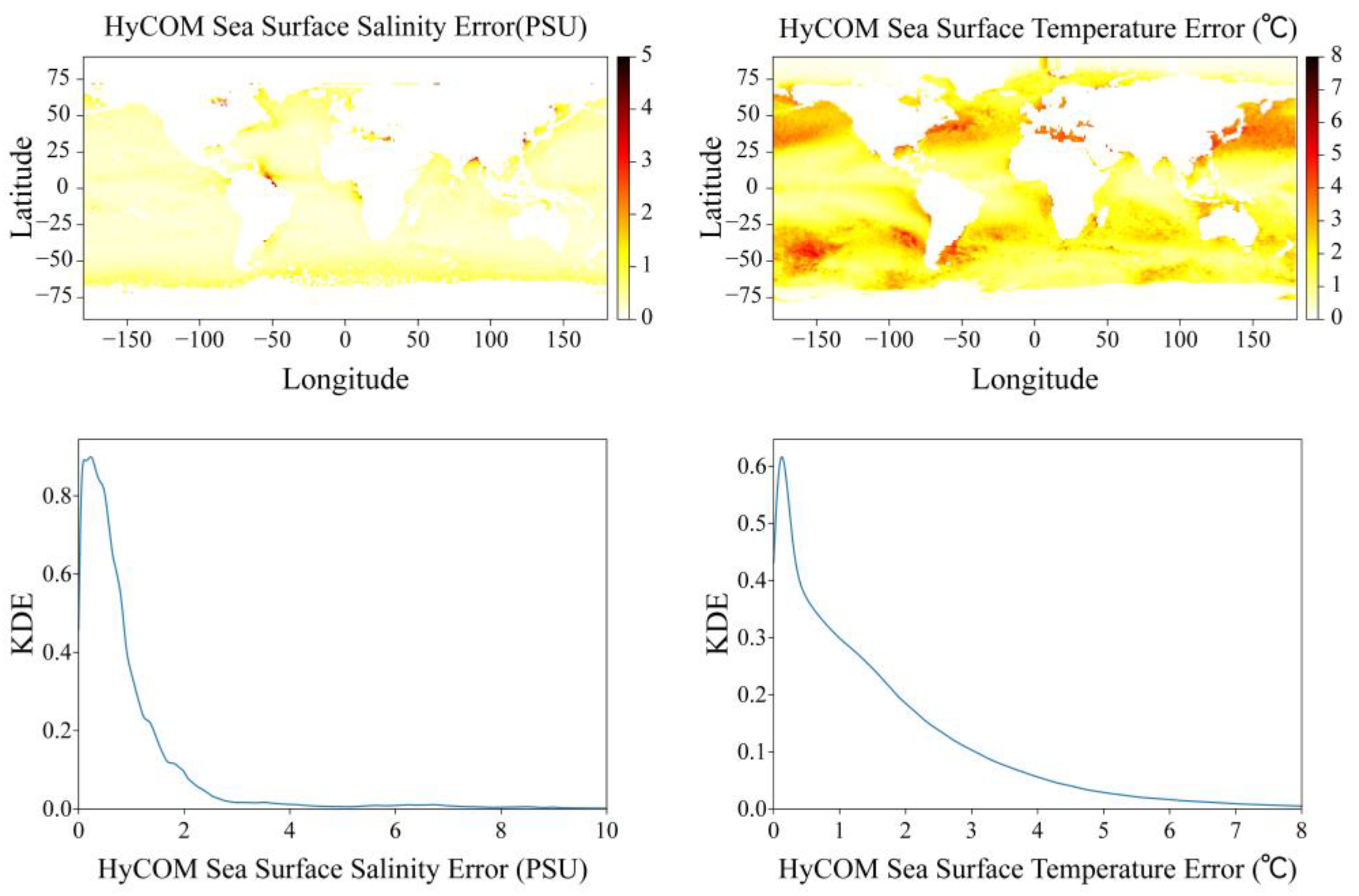
4. Comparison with HYCOM

Using the DSGNN deep learning model, we fuse and reconstruct the four types of satellite ocean data to produce high-resolution data with a resolution three times higher than that of the original data. Through a series of mathematical and statistical methods, we test the robustness and accuracy of the reconstructed datasets in Section 3, and the results are satisfactory. So, how does this model compare to traditional numerical ocean models? Machine learning methods, especially deep learning technology, are increasingly widely used in the field of marine science, and an important point is that there is a trend in mutual complement and combination with numerical models. The HYCOM is a very widely used marine numerical model and provides 1/12° output results, which have a similar resolution to that of our reconstructed datasets. We also take the EN4.2.2 dataset as the true value and calculate the annual error scatters and KDE of the reconstructed and HYCOM datasets, respectively. Figure 8 shows the annual error scatters and KDE of the DSGNN model, and Figure 9 shows the results of the HYCOM.

These two figures present a comparison between the HYCOM and DSGNN for the SSS and SST, respectively. The distribution of error scatters illustrates a close comparison between the reconstructed high-resolution and HYCOM sea surface data, indicating that the DSGNN datasets exhibit comparable levels of accuracy with those of the HYCOM. The results of the DSGNN are slightly worse than those of the HYCOM, but they are basically at the same level. The KDE curves of both the SST and SSS for the HYCOM are narrower than those for the DSGNN, and the peak of the HYCOM is more concentrated in the smaller value interval, which indicates that the errors of the HYCOM are more focused and stable than those of the DSGNN. In addition, the error spatial distribution of the two also presents interesting characteristics. For example, the error scatters of the reconstructed SST are evenly distributed in space, while the HYCOM are concentrated in the mid-latitude seas of the Northern and Southern Hemispheres. This may be due to an inherent bias in the numerical model. Although the effect of the DSGNN model is slightly worse than that of the HYCOM, the computing resources consumed by the DSGNN operation are far less than that of the HYCOM, which is also the biggest advantage of the deep learning model.

5. Discussion

In this study, we fuse four types of satellite ocean datasets in sea surface: the SST, SSS, SLA and ADT. Is the fusion and reconstruction of multi-source data more effective than single data? As we know, they are the four parameters commonly used in ocean satellite data, and there is a close interaction between them. Two-dimensional satellite data can be written in the mathematical form of a two-dimensional fluctuation conduction:

$${\displaystyle \frac{{\mathsf{\partial }}^2{K}_i}{\mathsf{\partial }{x}^2}}-{\sigma }_1^2({\displaystyle \frac{{\mathsf{\partial }}^2{K}_1}{\mathsf{\partial }{x}^2}}+{\displaystyle \frac{{\mathsf{\partial }}^2{K}_2}{\mathsf{\partial }{y}^2}})=f_1(K_1,K_2,K_3,K_4)$$

(10)

where K₁, K₂, K₃, and K₄ represent the data of the SST, SSS, SLA, ADT, respectively, and f₁, f₂, f₃, and f₄ represent the relationship between external inputs. In the ocean, there are complex interactions among the SST, SSS, SLA, and ADT. First, the temperature and salinity distribution of the ocean surface affects the variation in the ocean surface height. Changes in temperature and salinity lead to changes in seawater density, which, in turn, affect anomalous changes in the ocean surface height. This interrelationship between temperature and salinity and ocean surface height is referred to as ocean thermal and dynamical coupling. Second, anomalous changes in the ocean surface height affect the mixing and transport processes of seawater, which, in turn, affect the temperature and salinity distributions. This interrelationship between the ocean surface height and temperature and salinity distribution is referred to as ocean dynamics and physical coupling. Thus, the interactions between the SST, SSS, SLA, and ADT constitute a complex coupling process in the ocean system.

The seawater transport process is a complex process with strong nonlinear characteristics. The nonlinearity of the ocean equations of motion, the interactions between temperature and salinity, and the nonlinear nature of the boundary conditions work together to cause the seawater temperature and salinity transport process to exhibit a highly complex and nonlinear behavior. To solve such nonlinear processes, the following relationship must be solved:

$${\overline{K}}_{1,2,3,4}=-\mathsf{\Phi }\prime (K_{1,2,3,4})$$

(11)

Such complex processes do not have continuous dependencies, and fitting such processes using neural networks is very complex. Such a map is very difficult to find since there is no consistent uncertainty quantification and uniform data quality control for these variables themselves. In order to degrade such a problem, we unify the gridded data as described earlier, i.e., discretize it into a process such as the one below:

$$\mathsf{\Phi }(t,x)={\mathsf{\Phi }}_1(t)\left[\begin{array}{c}{\phi }_1(K_1)\\ {\phi }_2(K_2)\\ {\phi }_3(K_3)\\ {\phi }_4(K_4)\end{array}\right]$$

(12)

The study of lattice-point dynamical systems has shown that when Φ satisfies some conditions, such a discrete relation has a global attractor and also at least a local continuous dependence. This can bring a very large benefit for neural network fitting in this paper. Figure 10 compares the results with and without discrete spatial encoding. The same model with the discretization method exhibits a more rapid rate of convergence and lower steady-state loss values on the loss function curve. This faster convergence rate indicates that the DSGNN is more effective in tuning the model parameters due to its spatial discretization technique, which allows the network to handle the spatial features of marine scientific data more efficiently, thus obtaining better results at earlier iterations.

It is necessary to explain the complexity of the model. Firstly, we should define the parameters of spatial discretization encoding: the number of discrete points in two independent directions is denoted as n_x and n_y, respectively. Under this encoding strategy, the total number of discrete points across the entire space is calculated as follows: n_x × n_y. These discrete points directly influence the input dimensions of the embedding layer or the fully connected layer in the neural network model. Within the model’s architecture, it is assumed that the computational time complexity of the weight matrix of the first layer is t₁, while the total computational time complexity of all subsequent layers is t₂. Therefore, in the case of discrete encoding, the overall time complexity of the model can be represented as n_x × n_y × t₁ + t₂. It is noteworthy that the complexity of this issue is also affected by the number of fully connected layers and their depth within the neural network.

6. Conclusions

This study introduces a novel approach to satellite data fusion through the implementation of the Discrete Satellite Gridding Neural Network (DSGNN), which was designed to enhance the accuracy and predictive capabilities of oceanographic parameter data by employing a unified discrete grid processing technique. The DSGNN processes satellite data by scattering the positional information of various elements within different grids into a standardized specific position vector, followed by the application of a neural network model for data fusion and prediction. This methodology effectively improves the spatial resolution of the data, allowing for a more nuanced understanding of the ocean’s physical state.

The analysis of reconstructed satellite datasets concerning the SST, SSS, SLA, and ADT has demonstrated the superior performance of the DSGNN. It has exhibited consistency and reliability in error analysis across different seasons and oceanic regions, proving effective in various oceanic conditions. This consistency validates the applicability and efficacy of the DSGNN on a global scale. The methodological advancement of the DSGNN, particularly when compared to classical models such as the HYCOM, lies in its ability to learn complex nonlinear relationships between image blocks through multi-layer nonlinear mapping, thereby extracting advanced features and patterns from satellite data.

Furthermore, the high-resolution data fusion capabilities of the DSGNN have significant implications for the monitoring and modeling of oceanic phenomena over time. The high-resolution data fusion capabilities of the DSGNN can help address many of the current challenges in oceanographic research, from the study of small-scale oceanic processes to the monitoring of long-term climate trends. The speed of data processing and the consumption of computing resources are much less than that of the traditional ocean numerical model. In conclusion, the introduction of the DSGNN represents an advancement in the field of satellite data fusion for oceanography. Of course, the DSGNN is still a very rudimentary deep learning model as, for example, the accuracy of its output results is lower than that of the HYCOM, and it can only generate sea surface data at present. In the future, we hope to use more complex models instead of simple fully connected neural networks and further explore the ability to reconstruct datasets below the sea surface based on transfer learning and other methods.

References

1. Zhao, Q.; Yu, L.; Du, Z.; Peng, D.; Hao, P.; Zhang, Y.; Gong, P. An overview of the applications of earth observation satellite data: Impacts and Future Trends. Remote Sens. 2022, 14, 1863. [Google Scholar] [CrossRef]
2. Ban, Y.; Gong, P.; Giri, C. Global land cover mapping using earth observation satellite data: Recent progresses and challenges. ISPRS J. Photogramm. Remote Sens. 2015, 103, 1–6. [Google Scholar] [CrossRef]
3. Kuenzer, C.; Ottinger, M.; Wegmann, M.; Guo, H.; Wang, C.; Zhang, J.; Dech, S.; Wikelski, M. Earth observation satellite sensors for biodiversity monitoring: Potentials and bottlenecks. Int. J. Remote Sens. 2014, 35, 6599–6647. [Google Scholar] [CrossRef]
4. Anderson, K.; Ryan, B.; Sonntag, W.; Kavvada, A.; Friedl, L. Earth observation in service of the 2030 Agenda for sustainable development. Geo-Spatial Inf. Sci. 2017, 20, 77–96. [Google Scholar] [CrossRef]
5. De Grave, C.; Verrelst, J.; Morcillo-Pallarés, P.; Pipia, L.; Rivera-Caicedo, J.P.; Amin, E.; Moreno, J. Quantifying vegetation biophysical variables from the Sentinel-3/FLEX tandem mission: Evaluation of the synergy of OLCI and FLORIS data sources. Remote Sens. Environ. 2020, 251, 112101. [Google Scholar] [CrossRef]
6. Notti, D.; Giordan, D.; Caló, F.; Pepe, A.; Zucca, F.; Galve, J.P. Potential and limitations of open satellite data for flood mapping. Remote Sens. 2018, 10, 1673. [Google Scholar] [CrossRef]
7. Wang, S.; Jing, Z.; Wu, L.; Cai, W.; Chang, P.; Wang, H.; Yang, H. El Niño/Southern Oscillation inhibited by submesoscale ocean eddies. Nat. Geosci. 2022, 15, 112–117. [Google Scholar] [CrossRef]
8. Høyer, J.L.; She, J. Optimal interpolation of sea surface temperature for the North Sea and Baltic Sea. J. Mar. Syst. 2007, 65, 176–189. [Google Scholar] [CrossRef]
9. Gunes, H.; Rist, U. Spatial resolution enhancement/smoothing of stereo–particle-image-velocimetry data using proper-orthogonal-decomposition–based and Kriging interpolation methods. Phys. Fluids A 2007, 19, 064101. [Google Scholar] [CrossRef]
10. Liu, X.; Wang, M. Gap filling of missing data for VIIRS global ocean color products using the DINEOF method. IEEE Trans. Geosci. Remote Sens. 2018, 56, 4464–4476. [Google Scholar] [CrossRef]
11. Miles, T.N.; He, R. Temporal and spatial variability of Chl-a and SST on the South Atlantic Bight: Revisiting with cloud-free reconstructions of MODIS satellite imagery. Cont. Shelf Res. 2010, 30, 1951–1962. [Google Scholar] [CrossRef]
12. Jouini, M.; Lévy, M.; Crépon, M.; Thiria, S. Reconstruction of satellite chlorophyll images under heavy cloud coverage using a neural classification method. Remote Sens. Environ. 2013, 131, 232–246. [Google Scholar] [CrossRef]
13. Krasnopolsky, V.; Nadiga, S.; Mehra, A.; Bayler, E.; Behringer, D. Neural networks technique for filling gaps in satellite measurements: Application to ocean color observations. Comput. Intell. Neurosci. 2016, 2016, 6156513. [Google Scholar] [CrossRef]
14. Maimaitijiang, M.; Ghulam, A.; Sidike, P.; Hartling, S.; Maimaitiyiming, M.; Peterson, K.; Shavers, E.; Fishman, J.; Peterson, J.; Kadam, S.; et al. Unmanned Aerial System (uas)-based phenotyping of soybean using multi-sensor data fusion and Extreme Learning Machine. ISPRS J. Photogramm. Remote Sens. 2017, 134, 43–58. [Google Scholar] [CrossRef]
15. Ouala, S.; Fablet, R.; Herzet, C.; Chapron, B.; Pascual, A.; Collard, F.; Gaultier, L. Neural network based Kalman filters for the Spatio-temporal interpolation of satellite-derived sea surface temperature. Remote Sens. 2018, 10, 1864. [Google Scholar] [CrossRef]
16. Goly, A.; Teegavarapu, R.S.; Mondal, A. Development and evaluation of statistical downscaling models for monthly precipitation. Earth Interact. 2014, 18, 1–28. [Google Scholar] [CrossRef]
17. Sachindra, D.A.; Ahmed, K.; Rashid, M.M.; Shahid, S.; Perera, B.J.C. Statistical downscaling of precipitation using machine learning techniques. Atmos. Res. 2018, 212, 240–258. [Google Scholar] [CrossRef]
18. Jiang, Y.; Yang, K.; Shao, C.; Zhou, X.; Zhao, L.; Chen, Y.; Wu, H. A downscaling approach for constructing high-resolution precipitation dataset over the Tibetan Plateau from ERA5 reanalysis. Atmos. Res. 2021, 256, 105574. [Google Scholar] [CrossRef]
19. Dalla Mura, M.; Prasad, S.; Pacifici, F.; Gamba, P.; Chanussot, J.; Benediktsson, J.A. Challenges and opportunities of multimodality and data fusion in remote sensing. Proc. IEEE 2015, 103, 1585–1601. [Google Scholar] [CrossRef]
20. Schmitt, M.; Zhu, X.X. Data Fusion and remote sensing: An ever-growing relationship. IEEE Geosci. Remote Sens. Mag. 2016, 4, 6–23. [Google Scholar] [CrossRef]
21. Abdikan, S.; Balik Sanli, F.; Sunar, F.; Ehlers, M. A comparative data-fusion analysis of multi-sensor satellite images. Int. J. Digit. Earth 2012, 7, 671–687. [Google Scholar] [CrossRef]
22. Smilde, A.K.; Måge, I.; Næs, T.; Hankemeier, T.; Lips, M.A.; Kiers, H.A.; Acar, E.; Bro, R. Common and distinct components in data fusion. J. Chemom. 2017, 31, e2900. [Google Scholar] [CrossRef]
23. Park, H.; Kim, K.; Lee, D.k. Prediction of severe drought area based on Random Forest: Using satellite image and topography data. Water 2019, 11, 705. [Google Scholar] [CrossRef]
24. Mountrakis, G.; Im, J.; Ogole, C. Support vector machines in remote sensing: A Review. ISPRS J. Photogramm. Remote Sens. 2011, 66, 247–259. [Google Scholar] [CrossRef]
25. Huang, X.; Wen, D.; Xie, J.; Zhang, L. Quality assessment of Panchromatic and multispectral image fusion for the ZY-3 satellite: From an information extraction perspective. IEEE Geosci. Remote Sens. Lett. 2014, 11, 753–757. [Google Scholar] [CrossRef]
26. Cracknell, M.J.; Reading, A.M. Geological mapping using remote sensing data: A comparison of five machine learning algorithms, their response to variations in the spatial distribution of training data and the use of explicit spatial information. Comput. Geosci. 2014, 63, 22–33. [Google Scholar] [CrossRef]
27. Wang, C.; Wang, H. Cascaded feature fusion with multi-level self-attention mechanism for object detection. Pattern Recognit. 2023, 138, 109377. [Google Scholar] [CrossRef]
28. Minnett, P.J.; Alvera-Azcarate, A.; Chin, T.M.; Corlett, G.K.; Gentemann, C.L.; Karagali, I.; Li, X.; Marsouin, A.; Marullo, S.; Maturi, E.; et al. Half a century of satellite remote sensing of sea-surface temperature. Remote Sens. Environ. 2019, 233, 111366. [Google Scholar] [CrossRef]
29. Mignot, J.; de Boyer Montégut, C.; Lazar, A.; Cravatte, S. Control of salinity on the mixed layer depth in the world ocean: 2. Tropical areas. J. Geophys. Res. Oceans 2007, 112. [Google Scholar] [CrossRef]
30. Nardelli, B.B.; Verbrugge, G.N.; Cotroneo, Y.; Zambianchi, E.; Iudicone, D. Southern ocean mixed-layer seasonal and interannual variations from combined satellite and In Situ data. J. Geophys. Res. Oceans 2017, 122, 10042–10060. [Google Scholar] [CrossRef]
31. Reynolds, R.W.; Smith, T.M.; Liu, C.; Chelton, D.B.; Casey, K.S.; Schlax, M.G. Daily high-resolution-blended analyses for sea surface temperature. J. Clim. 2007, 20, 5473–5496. [Google Scholar] [CrossRef]
32. NCAR. SST Data: NOAA High-Resolution (0.25 × 0.25) Blended Analysis of Daily SST and Ice, OISSTv2. Climate Data Guide. Available online: https://climatedataguide.ucar.edu/climate-data/sst-data-noaa-high-resolution-025x025-blended-analysis-daily-sst-and-ice-oisstv2 (accessed on 14 August 2024).
33. Boutin, J.; Reul, N.; Koehler, J.; Martin, A.; Catany, R.; Guimbard, S.; Rouffi, F.; Vergely, J.L.; Arias, M.; Chakroun, M.; et al. Satellite-based sea surface salinity designed for ocean and climate studies. J. Geophys. Res. Oceans 2021, 126, e2021JC017676. [Google Scholar] [CrossRef]
34. Srokosz, M.; Banks, C. Salinity from space. Weather 2018, 74, 3–8. [Google Scholar] [CrossRef]
35. Banks, C.J.; Calafat, F.M.; Shaw, A.G.P.; Snaith, H.M.; Gommenginger, C.P.; Bouffard, J. A new daily quarter degree sea level anomaly product from CryoSat-2 for ocean science and applications. Sci. Data 2023, 10, 477. [Google Scholar] [CrossRef]
36. Amos, C.M.; Castelao, R.M. Influence of the El Niño-Southern Oscillation on SST fronts along the west coasts of North and South America. J. Geophys. Res. Oceans 2022, 127, e2022JC018479. [Google Scholar] [CrossRef]
37. Bingham, R.J.; Haines, K.; Hughes, C.W. Calculating the ocean’s mean dynamic topography from a mean sea surface and a geoid. J. Atmos. Ocean. Technol. 2007, 25, 1808–1822. [Google Scholar] [CrossRef]
38. Atkinson, C.P.; Rayner, N.A.; Kennedy, J.J.; Good, S.A. An integrated database of ocean temperature and salinity observations. J. Geophys. Res. Oceans 2014, 119, 7139–7163. [Google Scholar] [CrossRef]
39. Chassignet, E.P.; Hurlburt, H.E.; Smedstad, O.M.; Halliwell, G.R.; Hogan, P.J.; Wallcraft, A.J.; Baraille, R.; Bleck, R. The HYCOM (Hybrid Coordinate Ocean Model) data assimilative system. J. Mar. Syst. 2007, 65, 60–83. [Google Scholar] [CrossRef]
40. Dash, R.; Paramguru, R.L.; Dash, R. Comparative analysis of supervised and unsupervised discretization techniques. Int. J. Adv. Sci. Technol. 2011, 2, 29–37. [Google Scholar]
41. Garcia, S.; Luengo, J.; Sáez, J.A.; Lopez, V.; Herrera, F. A survey of discretization techniques: Taxonomy and empirical analysis in supervised learning. IEEE Trans. Knowl. Data Eng. 2012, 25, 734–750. [Google Scholar] [CrossRef]
42. Müller, T.; Evans, A.; Schied, C.; Keller, A. Instant neural graphics primitives with a multiresolution hash encoding. ACM Trans. Graphics (TOG) 2022, 41, 102. [Google Scholar] [CrossRef]
43. Pargent, F.; Pfisterer, F.; Thomas, J.; Bischl, B. Regularized target encoding outperforms traditional methods in supervised machine learning with high cardinality features. Comput. Stat. 2022, 37, 2671–2692. [Google Scholar] [CrossRef]
44. Yang, P.; Jing, Z.; Sun, B.; Wu, L.; Qiu, B.; Chang, P.; Ramachandran, S. On the upper-ocean vertical eddy heat transport in the Kuroshio extension. Part I: Variability and dynamics. J. Phys. Oceanogr. 2021, 51, 229–246. [Google Scholar] [CrossRef]
45. Sang, Y.; Qi, H.; Li, K.; Jin, Y.; Yan, D.; Gao, S. An effective discretization method for disposing high-dimensional data. Inf. Sci. 2014, 270, 73–91. [Google Scholar] [CrossRef]
46. Franc, V.; Fikar, O.; Bartos, K.; Sofka, M. Learning data discretization via convex optimization. Mach. Learn. 2018, 107, 333–355. [Google Scholar] [CrossRef]
47. Spencer, C.J.; Yakymchuk, C.; Ghaznavi, M. Visualizing data distributions with kernel density estimation and reduced chi-squared statistic. Geosci. Front. 2017, 8, 1246–1252. [Google Scholar] [CrossRef]
48. Jung, S.; Yoo, C.; Im, J. High-Resolution Seamless Daily Sea Surface Temperature Based on Satellite Data Fusion and Machine Learning over Kuroshio Extension. Remote Sens. 2022, 14, 575. [Google Scholar] [CrossRef]
49. Kumar, C.; Podestá, G.; Kilpatrick, K.; Minnett, P. A machine learning approach to estimating the error in satellite sea surface temperature retrievals. Remote Sens. Environ. 2021, 255, 112227. [Google Scholar] [CrossRef]
Figure 1. Schematic diagram of matrix construction for spatial discretization method.
Remotesensing 16 03020 g001
Figure 2. Neural network regression of processing dataset task.
Remotesensing 16 03020 g002
Figure 3. High-resolution reconstruction of satellite imagery: generating new (a) ADT, (b) SLA, (c) SSS and (d) SST datasets in 1/12° (date: 1 January 2022).
Remotesensing 16 03020 g003
Figure 4. The error scatters of high-resolution reconstructed (a,e,i,m) ADT, (b,f,j,n) SLA, (c,g,k,o) SSS and (d,h,l,p) SST compared to the EN4.4.2 datasets. From the top row to the bottom are the interpolation results from 1 January, 1 April, 1 July and 1 October, respectively (the averages from 2010 to 2023).
Remotesensing 16 03020 g004
Figure 5. Global monthly averaged Root Mean Square Error (RMSE) of high-resolution reconstructed (a) ADT, (b) SLA, (c) SSS and (d) SST compared to EN4.4.2 datasets (average from 2010 to 2023).
Remotesensing 16 03020 g005
Figure 6. Kernel density estimation (KDE) curves of loss errors for high-resolution reconstructed (a) ADT, (b) SLA, (c) SSS and (d) SST datasets.
Remotesensing 16 03020 g006
Figure 7. Loss curves for reconstructed SST, SSS, ADT, and SLA data in different regions (North Atlantic, South Atlantic, Indian, North Pacific, and South Pacific Oceans) of the global ocean. The left column includes data from different months, and the right includes data from different years.
Remotesensing 16 03020 g007
Figure 8. The annual error scatters and KDE of high-resolution reconstructed SST, SSS, ADT, and SLA data compared to the EN4.4.2 datasets (the average from 2010 to 2023).
Remotesensing 16 03020 g008
Figure 9. The same data as those in Figure 8 but for the HYCOM datasets.
Remotesensing 16 03020 g009
Figure 10. Loss curves of deep neural network models with and without discretization method in training.
Remotesensing 16 03020 g010