First Release of the Optimal Cloud Analysis Climate Data Record from the EUMETSAT SEVIRI Measurements 2004–2019

Abstract

Clouds are key to understanding the atmosphere and climate, and a long series of satellite observations provide invaluable information to study their properties. EUMETSAT has published Release 1 of the Optimal Cloud Analysis (OCA) Climate Data Record (CDR), which provides a homogeneous time series of cloud properties of up to two overlapping layers, together with uncertainties. The OCA product is derived using the 15 min Spinning Enhanced Visible and Infrared Imager (SEVIRI) measurements onboard Meteosat Second Generation (MSG) in geostationary orbit and covers the period from 19 January 2004 until 31 August 2019. This paper presents the validation of the OCA cloud-top pressure (CTP) against independent lidar-based estimates and the quality assessment of the cloud optical thickness (COT) and cloud particle effective radius (CRE) against a combination of products from satellite-based active and passive instruments. The OCA CTP is in good agreement with the CTP sensed by lidar for low thick liquid clouds and substantially below in the case of high ice clouds, in agreement with previous studies. The retrievals of COT and CRE are more reliable when constrained by solar channels and are consistent with other retrievals from passive imagers. The resulting cloud properties are stable and homogeneous over the whole period when compared against similar CDRs from passive instruments. For CTP, the OCA CDR and the near-real-time OCA products are consistent, allowing for the use of OCA near-real time products to extend the CDR beyond August 2019.

1. Introduction

Clouds are very important for monitoring weather but also climate change [1]. They can be observed from the ground but also from above using instruments onboard satellites. EUMETSAT has operated its geostationary Meteosat satellites series since the early 1980s [2]. Since that time, there have continuously been prime Meteosat satellites located at 0° longitude and observing the Earth in a circle, with about a 65° radius around the satellite. Each Meteosat carries several instruments to monitor the Earth’s atmosphere. Among the instruments, there has always been a passive imager. The Meteosat imagers evolved with time, but they have always provided images in several channels spread over the infrared (IR) and visible (VIS) parts of the spectrum. The Meteosat Visible and InfraRed Imager (MVIRI) was mounted onboard Meteosat First Generation (MFG) satellites, observing the Earth on three channels every 30 min at a resolution of five kilometers (km). The Spinning Enhanced Visible and InfraRed Imager (SEVIRI) flies onboard Meteosat Second Generation (MSG) satellites and observes the Earth on 12 channels every 15 min. Finally, in December 2022, the Flexible Combined Imager (FCI) appeared in Meteosat Third Generation satellites (MTG); it observes the Earth every 10 min on 16 channels.

Although several cloud products retrieved from imagers exist, the Optimal estimation algorithm for Cloud Analysis (OCA, [3]) is quite unique. It was first developed as a research study awarded to the Rutherford Appleton Laboratory (RAL) in 1997 and implemented within the EUMETSAT near-real-time (NRT) facility as an MSG product in 2013. OCA uses SEVIRI images to retrieve cloud information such as cloud-top pressure (CTP), cloud optical thickness (COT), cloud effective radius (CRE), and cloud phase at pixel level. While the detection of multi-layer (i.e., “overlapping”) clouds is quite a common output in cloud schemes, a key characteristic of the OCA algorithm is the ability to estimate at the instrument spatial and temporal sampling the cloud properties of up to two layers, in favorable situations. This is a distinguishing feature of this dataset in comparison to other available long time series cloud products from passive imagers such as SEVIRI. It also provides an estimation of the retrieval uncertainty, which can be used to provide a quality control filter that could be propagated in downstream applications and algorithms such as, e.g., the height assignment of atmospheric motion vectors (AMVs).

To generate a homogeneous data record over the period 2004–2019, the OCA algorithm has been adapted for standalone reprocessing, using a new cloud mask [4], ERA-Interim reanalysis data instead of ECMWF NRT model forecast. The output product’s format has been redesigned and provides NetCDF instead of GRIB.

This paper presents the first release of the OCA CDR together with its main validation outcome. The aim is to provide a fully consistent long-term data record employing the most up-to-date available version of the NRT OCA algorithm, using consistent auxiliary data and SEVIRI Level 1.5 images as inputs. The OCA CDR covers a 15-year period of SEVIRI measurements onboard Meteosat-8, -9, -10, and -11 platforms during the period from January 2004 until the end of August 2019 (limit of the ERA-Interim data record). The completeness of the retrieval, the stability in time, and the presence of the typical geographical and seasonal cloud features are first verified by checking the products’ temporal consistency. OCA cloud properties are then evaluated against other retrievals based on the SEVIRI and MODIS observations, such as the CLAAS-3 and MODIS L3, while CTP is validated against independent satellite observations from active instruments onboard polar-orbiting platforms from the A-Train constellation. The CDR is finally compared against the EUMETSAT’s OCA NRT archived product.

This paper is organized as follows: Section 2 provides a brief description of the OCA algorithm and of the ancillary data used in the CDR’s generation. Section 3 provides an overview of the spatial and temporal extension of the OCA CDR. Section 4 describes the datasets used for the evaluation of the quality of the OCA CDR and Section 5 discusses the results of the comparisons against these reference datasets. Finally, Section 6 provides an overview of the limitations of the OCA CDR and the planned improvements.

2. Materials and Methods

2.1. Brief Description of the OCA Algorithm

A detailed description of the OCA algorithm is available in [3,5,6]. An overview of the main characteristics is presented in this section.

OCA simultaneously retrieves cloud-top pressure, total cloud optical thickness and the CRE of the liquid water droplets or ice crystals near the cloud top for up to two overlapping cloud layers. A cloud layer is modeled in OCA as a vertically homogeneous and geometrically infinitely thin single layer, with a COT defined at 0.55 μm, and a single microphysical phase. The CRE retrieved by OCA is defined as the ratio of the third to the second moment of the cloud particle size distribution and the quantity represents the distribution-weighted mean particle size effectively seen by radiation. Ice crystals are represented as severely roughened aggregates of solid columns [7].

Together with the three variables defining the cloud state, two further variables are included in the state vector of the optimal estimation algorithm: the temperature of the underlying surface (Tskin), because of the strong dependence of almost all thermal IR channels in some cloud conditions, and the fractional cloud cover (CFR).

An optimal estimation approach is used to retrieve the cloud state parameters as a function of measurements in an adjustable number of VIS/IR channels. Prior information is provided for each state variable but with no constraint except for CFR, which is kept close to the value of 1 and Tskin for which ERA-Interim values are used with an error of 1 K over sea and 3 K over land. It was found that the degrees of freedom available in the measurements do not provide enough information, except for particular conditions, to allow for the CFR to be independently estimated. As result, if not constrained to the prior information, CFR values result most often as a false trade-off with COT or CTP or both. As further motivation, for small pixels, the true distribution of fractional cloud cover is highly peaked at values zero and one and the assumption of CFR = 1 for cloud detected pixel is a relatively good one. The measurement covariance matrix includes error parameters estimated based on instrument noise and predominant modelling errors.

Auxiliary information necessary to translate the cloud state into imager measurements is provided via a set of external files and parameters. This set includes atmospheric meteorological information from a forecast model, surface properties, the lookup tables (LUTs) for atmospheric gaseous absorption and emission for all SEVIRI channels computed with the radiative transfer for TOVS (RTTOV version 11.2, [8]) and LUTs of clouds radiative properties pre-calculated using DISORT [9,10].

A simple, fast forward model calculates the interactions between a cloud layer, the absorbing atmosphere above and below the cloud and the Lambertian surface in terms of simple reflecting streams including the Jacobians of the state variables with respect to the input measurements. The algorithm adjusts the cloud state to minimize, under certain constraints, the difference between the measurements and their equivalents calculated with the fast forward model and the difference between the value in the state variables and their a priori assumptions. This difference is represented by the system cost or penalty function.

This simple model is not able to represent correctly overlapping cloud layers, and this is reflected in a higher solution cost after convergence for actual multi-layer scenes. Thermal IR WV channels (6.3–7.3 μm) are vital to this signature, as the absorption taking place between the layers is inconsistent with a single-layer cloud, but short-wave channels also offer vital information as they are able to better constrain the total optical depth of the multiple cloud layers. The OCA algorithm takes advantage of the high solution cost (and some other measurement-based indicators) to detect multi-layer clouds. Pixels thus detected are reprocessed using a simple two-layer (2L) model and IR-only channels (see [3] for the details).

Each retrieved cloud property comes with an error estimate that is calculated by propagation of the modelled errors in the input parameters as part of the optimal estimation framework. Contributing to this error estimate is the characterization of scene and cloud properties in the OCA forward model, the knowledge of measurement errors, and the treatment of prior information. Section 5 provides an indication of the reliability of such an error estimate by comparing it to the real retrieval error with respect to a reference dataset. In addition, there is, per pixel, an overall quality indicator based on the cost of the retrieval. While the error estimates are derived for, and can be applied to, each cloud property separately, the overall quality indicator is applicable to all retrieved cloud properties for the pixel.

2.2. The Input Data for the Reprocessing

2.2.1. SEVIRI Data

Cloud properties are derived using images acquired from the four SEVIRI instruments onboard the series of MSG satellites. The OCA CDR provides products derived every 15 min over the full disk, with maximum extents of 65°N–65°S and 65°W–65°E around the nominal sub-satellite point (SSP) (see

Table 1. Temporal information on which Meteosat platforms located at 0° embarked the SEVIRI instrument throughout the CDR period (2004–2019).

Satellite	Start Date	End Date
Meteosat-8	19 January 2004	11 April 2007
Meteosat-9	11 April 2007	21 January 2013
Meteosat-10	21 January 2013	20 February 2018
Meteosat-11	20 February 2018	31 August 2019

) for the prime satellite.

Some of the MSG satellites were moved over the Indian Ocean but the OCA CDR only includes products from the MSG 0° missions. The spatial coverage is given in Figure 1. The retrieval is carried out at full spatial resolution, with a nominal pixel size at an SSP of 3 km. Due to normal operation changes (satellite maintenance) to the prime satellite, few products are generated using the current backup platform. For this reason, some products are generated at an SSP of 3.4° west and others at 9.5° East (Figure 1). The information about the current SSP is not included in the product in this release, but each pixel contains its latitude and longitude.

SEVIRI level 1.5 images are taken from the EUMETSAT near-real-time archive system (http://data.eumetsat.int, accessed on 2 August 2024) with the calibrations therein applied. For the thermal infrared channels (3.9 to 13.3 µm), no further adjustment has been made. The three short-wave solar channels at 0.6, 0.8, and 1.6 µm are corrected for a known significant calibration bias according to the analysis of SEVIRI-MODIS matchups [11]. Although the biases are known to drift somewhat and be slightly different between the SEVIRI instruments, a single value per channel has been used in the generation of this version of the CDR (1.08, 1.06, and 0.96 for channels 0.6 μm, 0.8 μm, and 1.6 μm, respectively).

2.2.2. Meteorological Data and RTTOV LUTs

The generation of the OCA CDR uses auxiliary inputs from meteorological and radiative transfer models.

The estimation of the atmospheric temperature and humidity profiles and ozone at the individual SEVIRI pixel’s location and time are extracted from ECMWF ERA-Interim reanalysis [12]. The 6 and 12 h reanalysis forecasts from the 0 and 12 UTC base times, leading to 4 forecast files per day (0, 6, 12, and 18 UTC) are used. The spatial resolution of the ERA-Interim forecast is 1° × 1°. The model values are linearly interpolated at the SEVIRI image in time and space.

OCA needs the clear sky transmittance and radiances that are computed using RTTOV version 11.2. RTTOV requires the model temperature, specific humidity, and ozone profiles to compute the lookup tables (LUTs) for the atmospheric emissivity and transmissivity for the infrared channels and the two-path transmissions for the short-wave channels.

The model reanalysis forecast and RTTOV data are then both used as input for the main OCA algorithm.

2.2.3. Cloud Mask

The OCA algorithm itself does not determine whether a SEVIRI pixel is cloudy or not. The cloud mask is obtained from SEVIRI measurements using an algorithm developed at MeteoSwiss within the Climate Monitoring Satellite Application Facility (CM SAF) [4]. The implemented scheme of the MeteoSwiss cloud mask is based on a Bayesian approach applied to a set of scores calculated exploiting only two solar (VIS) channels around 0.6 and 0.8 μm and one thermal IR channel around 10.8 μm. The algorithm also builds up a daily background reflectance map to assess potential clouds with higher reliability. The mask provides a cloud probability for 7 fixed steps for each SEVIRI pixel: 0, 25, 40, 50, 60, 75, and 100%. For the OCA CDR, all pixels with a cloud probability higher than 40% are considered cloudy and passed to OCA for retrieval. The cloud probability has been included in the OCA CDR to allow for users to further discriminate potentially dubious solutions.

2.2.4. Surface Properties

Interpretation of the solar reflectance measurements, even in cloudy situations, requires knowledge of the reflectivity of the underlying surface. An advantage of geostationary sensors is that they continually view the same ground locations so that, over a relatively short time, cloud-free daytime reflectance maps can be generated for the full disk. This is performed in NRT for the SEVIRI instruments and the resulting “Clear Sky Reflectance Maps” (CRM product) [13] can be obtained from the EUMETSAT archive. The NRT CRM stores the mean cloud-free top of atmosphere (TOA) reflectance for the three channels and they are updated, on a rolling basis, every day at 13:15 UTC. The archive of CRM is incomplete, as it has been affected by operational outages and differing archiving procedures over time. As surface reflectance is a slowly changing phenomenon, when the CRM of a specific day was missing, the algorithm selected the first available CRM for the same day in one of the following years. The principle behind this decision is that the surface reflectance depends strongly on the illumination conditions, i.e., on the season (assuming, of course, no major changes in the surface coverage). This choice does not have a significant impact on the OCA outputs.

3. The OCA CDR

The OCA CDR is described in detail in the CDR user guide [14]. The product includes information on cloud phase, cloud-top pressure, cloud optical thickness, and particle effective radius, and the input cloud mask for every SEVIRI pixel at the nominal 15 min frequency. Each retrieved cloud property comes with its associated relative error estimate. The CDR also provides additional information as metadata, such as several overall disk averages to allow for users to perform a quick check on the product’s quality.

The OCA CDR, with its combination of phases and layers, is different to traditional cloud products. To illustrate this, Figure 2 presents a pseudo-vertical cross-section of the OCA product for a sample of about 700 pixels in the west–east direction across Europe intersecting various cloud types; CTPs are shown as cloud-top heights (CTHs) (height in km) and the COTs as geometric vertical extent. The Figure 2 shows the presence of single-layer ice and liquid clouds, as well as two-layer clouds. The figure excludes information on CRE, error estimates, and the overall quality indicator.

3.1. Consistency of the OCA CDR Time Series

In this section, the OCA CDR is analyzed in terms of self-consistency, showing that the data record does not include unexpected gaps and that it is stable and homogeneous in time. The key retrieval variables of cloud properties are plotted and are shown for the complete spatial and temporal coverage. For this purpose, OCA CDR products were aggregated to daily and monthly means and re-gridded to a one-degree resolution. Hovmöller diagrams, covering the full period, were then produced from these aggregate files to provide a robust overview of the data record behavior over the complete time series.

Daily files on a grid of one-degree resolution are created using daylight hourly products (defined as having a solar zenith angle <80 degrees) from 09:00 to 15:00 UTC (seven products/day). The aggregation is carried out for observations within a 60° circle around the sub-satellite point to limit the inclusion of pixels with too high a zenith angle. Therefore, they can be defined as daylight aggregation products. This choice was made mainly to be able to better compare against other products only containing daytime microphysics retrievals. There are no artefacts due to nighttime retrieval for the CTP. A one-degree box is filled with an average value if at least 20% of the pixels in the box have been retrieved. This has the objective of avoiding upscaling grid points without a significant sample. To reduce the size of this re-gridded version of the OCA CDR, instead of computing averages for ice and liquid clouds separately, cloud properties have been aggregated into a single combined variable for each retrieved parameter. The fraction of ice, liquid, and two-layer pixels within a one-degree box is also saved. Two further sets of variables are calculated: one using all available retrievals and one (quality controlled or QC) only containing the OCA retrievals for which the final cost function and the retrieval errors for the cloud-top pressure are, respectively, less than 900 and 90 hPa. The thresholds are low enough so as to block the worse retrievals but large enough so as not to cause the rejection of too many pixels. With these thresholds, the rejection rate is about 5% at nighttime and 15% at daytime.

From the daylight aggregation files, a monthly aggregation file is created. Each OCA product contains a mask for each grid point, containing the ratio between the days with a valid retrieval and the number of days in the month. For instance, if a grid point in June 2005 (containing 30 days) comprises three daylight values, the value of the mask is 0.1 (10%) for that grid point. This mask will be applied to the monthly averaged variables to filter out pixels with a too low number of valid retrievals.

3.2. Monthly Cloud Properties

In Figure 3, the zonal averaged CTP over the latitude range −60° to +60° is shown using a filtering of 60% cloud retrieval threshold (lower panel).

The CTP time series is homogeneous and smooth over the period and does not exhibit any changes linked with changes in SEVIRI instruments. We clearly see the low-level stratus and cumulus clouds at about 20° latitude. There is a clear seasonal cycle showing more low clouds over the south 20° band going from about 850 hPa in June to 700 hPa in January. Over the tropics, the averaged CTP is higher located above about 500 hPa. At higher latitudes above 40°, the time series does not show any clear seasonal cycle and the zonal averaged CTP over the −60/60° bands is about 650 hPa.

For each cloud retrieved by OCA, a cloud type is associated. Three types are possible, i.e., a one-layer ice cloud, a one-layer water cloud, or two-layer clouds. Note than in the case of a two-layer cloud, OCA assumes the ice phase for the uppermost layer while no phase is specified for the underlying layer. As explained before, for the monthly averages, we computed the fraction of each cloud type: the one-layer water clouds dominate with between 50% and more than 70% frequency depending on the region; the one-layer ice clouds are around 30–40%, especially in the tropics and at high latitudes. The least occurring cloud type in OCA are the two-layer clouds with a fraction of about 20%, with the largest occurrences in the tropical regions associated with the anvils of large convective clouds. The distribution is very constant during the whole period and shows clear seasonal variations.

Finally, the total COT and CRE combined for all cloud types and zonal-averaged over the latitude range −60° to +60° are shown (Figure 4). The constant COT’s high value at −60° latitude is due to a combination of high viewing angles and surface conditions (such as sea or land ice) that make the retrieval highly unreliable.

3.3. Geographical Distribution of Cloud Parameters

The geographical distribution of the OCA cloud properties is shown in the Figure 5 as a monthly average.

OCA products show a good representation of the typical climatology of cloud types for this region of the Earth. We can see that most single-layer liquid water clouds are found over the oceans, in the stratocumulus and trade cumulus region off the west coast of Africa in the middle and southern Atlantic. Ice clouds are associated with high convection in the tropics, where the signature of individual deep convection cells is visible in the daily average. Mixed liquid and ice clouds can be found most often in the mid-latitude storm track. Two-layer clouds generally follow the area where ice clouds are mostly found, as this is where ice clouds more likely overlap with cloud layers below.

We can also see that a significant number of pixels rejected according to the quality control filters, discussed in Section 3.1, appear both over land and over water, often in areas of complex overlapping cloud conditions and challenging surface properties such as over deserts or in the vicinity of large convective systems. On a monthly average scale, the areas with the lowest number of usable products are mostly located over the dry subsidence areas in the tropical and subtropical regions.

The properties of the various cloud regimes as retrieved by OCA reflect their typical physical characteristics. Generally, high clouds with low top pressure are associated with ice crystals with a larger size of order of 25–30 μm while lower liquid water clouds have droplet size of less than 20 μm. The largest values of cloud optical thickness are found within deep convective systems and frontal systems in the mid latitudes. We can observe that there is a tendency for OCA to overestimate the amount of low-level clouds over deserts, which is visible in the daily and monthly averages. This is a side effect of using a cloud-conservative threshold in the cloud mask: misclassified cloudy areas over bright surfaces tend to be interpreted as low liquid clouds by the algorithm.

4. Validation against Other Independent Datasets

4.1. The Datasets Used for Validation

To validate and verify the quality of the OCA CDR retrievals, we used several products, ranging from independent observations of cloud properties to retrieval products from other instruments onboard both geostationary and polar-orbiting platforms.

The main source of independent measurements for the validation of cloud properties is the A-Train constellation, and in particular the active measurements from the CloudSat radar and Cloud–Aerosol Lidar and Infrared Pathfinder Satellite Observations (CALIPSO) lidar. The main sources for comparing OCA cloud properties against retrievals from other passive imager algorithms are the Moderate Resolution Imaging Spectroradiometer (MODIS) Level 2 (L2) and Level 3 (L3) products and The CLoud property dAtAset using SEVIRI, Edition 3 (CLAAS-3), two well-tested and validated cloud property data records. All the data used in this paper are be described in the following sections.

4.1.1. DARDAR

The raDAR/liDAR (DARDAR) algorithm [15,16] combines variational algorithm data from spaceborne radar, lidar, and infrared radiometers for cloud phase identification and the retrieval of ice cloud properties. The algorithm is applied to the instruments on the “A-Train” of satellites, which includes CALIPSO [17] (carrying a nadir-viewing two-wavelength, 532 and 1064 nm, polarization-sensitive lidar), CloudSat (a 94 GHz cloud profiling radar [18]), and the AQUA platform carrying the MODIS instrument [19].

The synergistic use of different instruments to retrieve the microphysical properties of ice clouds allows for combining the strengths of each instrument. Radars are less sensitive to small particles than lidars, but the latter are more sensitive to optically thin clouds and tend to be strongly attenuated by thick cloud layers. DARDAR can seamlessly retrieve the cloud properties between areas where one or more instruments are available using all available measurements and empirical constraints in an optimal estimation framework.

Given the capability of OCA retrievals to distinguish between single- and multi-layer situations, DARDAR allows for us to explore, in a fine vertical grid, the complete view of the vertical profile of a cloud layer. In this paper, we use the DARDAR feature mask and cloud retrieval (DARDAR-CLOUD and DARDAR-MASK files) as the main reference for defining single- and multi-layer cloud profiles, cloud phase, and cloud-top height of up to three overlapping cloud layers.

For the collocation between SEVIRI and A-Train observations including parallax correction, we use the A-Train Validation of Aerosol and Cloud Properties from SEVIRI (AVAC-X version 4.0) software, an updated version its precursor, AVAC-S, adapted to work with any generic geostationary satellite [20]. AVAC-X uses the CloudSat 2B-GEOPROF file as basis for the geolocation and alignment of geostationary and A-Train products.

To keep the computational load of the data processing reasonable, we selected a set of three days per month with one daytime and one nighttime orbit per day to run the validation. The chosen days are always about 10 days apart, around the 1st, the 10th and the 20th of the month, depending on their availability. The analyzed DARDAR granules cross the SEVIRI disk around 2 a.m. UTC and 3 a.m. UTC for the night overpasses and between 1 p.m. UTC and 2 p.m. UTC for the daytime overpasses. The selected DARDAR granules are close to the central part of the SEVIRI disk to facilitate the comparison between the instruments by excluding too large viewing angles to the east and west of the MSG sub-satellite point.

4.1.2. CALIPSO L3 GEWEX Cloud-Top Product

This gridded dataset is based on CALIPSO L2 cloud products and produced for the Global Energy and Water Cycle Experiment (GEWEX) Cloud Assessment (10.5067/CALIOP/CALIPSO/LID_L3_GEWEX_Cloud-Standard-V1-00, accessed on 2 August 2024). The L2 products are aggregated on a 1° × 1° grid in a set of monthly files covering the period 2006–2016 and divided into day-only, night-only, and day–night retrievals.

Different versions (flavors) of cloud-top products are available in each monthly file, suitable for different applications. The two relevant for the present analysis are the “TopLayer” and the “Passive” versions. The former selects only the topmost layer in each CALIPSO profile while the latter reports the cloud-top products at the level where clouds have an optical thickness larger than 0.3, as this is closer to what is likely to be sensed by a passive instrument like SEVIRI.

4.1.3. CLAAS-3

The time series consistency and the mean climatological features of the OCA CDR were analyzed through a comparison against another dataset based on SEVIRI measurements covering the same time span: the CM SAF CLoud property dAtAset using SEVIRI—Edition 3 (CLAAS-3) dataset [21]. This dataset contains retrieved cloud properties from inter-calibrated measurements of SEVIRI onboard the MSG satellites MSG-1, MSG-2, and MSG-3 covering the period 2004–2021. The EUMETSAT Satellite Application Facility on Climate Monitoring (CM-SAF, http://www.cmsaf.eu, accessed on 2 August 2024) produces the dataset.

The CLAAS-3 presents a substantial upgrade with respect to the previous CLAAS-2 dataset. In particular, the retrieval of the cloud-top pressure is now performed with a perceptron neural network [22] trained on a dataset collocation between SEVIRI and CALIOP, therefore representing a significant departure from methods relying on the direct simulation of cloud-affected radiances as employed by OCA. The CPP (cloud physical properties) algorithm [23] is used for the retrieval of cloud-top thermodynamic phase, cloud optical thickness, cloud particle effective radius, and liquid/ice water path. In this latest version of the dataset, assumption on the microphysical properties of liquid droplets and ice clouds have been modified. The CLAAS-3 validation report [24] provides ample discussion on the quality of the retrieval products against reference datasets.

In this report, we use the monthly mean Level 3 CLAAS-3 for the comparison of the cloud microphysics, optical thickness, and cloud-top pressure.

4.1.4. MODIS L3

We compare OCA CDR to the products from MODIS [19], such as cross-comparison between cloud properties retrievals from passive radiometers using similar spectral channels but onboard different platforms. The MODIS instrument flies onboard the TERRA and AQUA satellites, both on a polar sun-synchronous orbit with equatorial crossing times, respectively, of 10:30 a.m. in descending direction and 1:30 p.m. local solar time in ascending direction.

For the following evaluation, we use the gridded MODIS L3 datasets to compare the OCA CDR over the whole SEVIRI reprocessing period 2004–2019. The L3 TERRA MOD08_M3 (https://ladsweb.modaps.eosdis.nasa.gov/missions-and-measurements/products/MOD08_M3, accessed on 2 August 2024) and L3 AQUA MYD08_M3 (https://ladsweb.modaps.eosdis.nasa.gov/missions-and-measurements/products/MYD08_M3, accessed on 2 August 2024) collection 6.1 files contain monthly mean cloud, atmosphere, and aerosol retrieval parameters on a 1° × 1° resolution grid and for the entire globe. We averaged the retrievals from TERRA and AQUA to obtain a slightly more accurate daytime average using both the morning and afternoon equatorial crossing times. The sparse temporal sampling tends to bias the daytime MODIS product towards being representative of the local solar time, especially for the region between 23° north and 23° south. Poleward of these latitudes, the MODIS L3 data slowly become an average of several orbits roughly 100 min apart, and poleward of 77°, this leads to an effective daily average [25].

Based on a similar set of channels, MODIS and OCA products do differ somewhat not only due to the different spatial resolution and temporal resolution (

Table 2. Summary of the main differences in spatial and temporal resolution between L2 and L3 retrieval products from OCA-SEVIRI CDR and MODIS. OCA is provided to the users at the native SEVIRI resolution of 15 min (Level 2). The aggregation to monthly mean (Level 3) has been carried out for comparison purposes only.

	L2 Products Resolution		L3 Products Resolution
	Spatial	Temporal	Spatial	Temporal
OCA	3 km at nadir	15 min	1° × 1°	Monthly mean from 7 observations/day (hourly from 09Z to 15Z)
MODIS	1 km at nadir	Twice daily at low/mid latitudes	1° × 1°	Monthly mean from roughly 1 observation/day at low to mid latitudes

) and larger number of channels available in MODIS, but also due to the different retrieval approach for the same cloud parameters (see [26,27] and references herein for an overview of the core MODIS cloud product algorithms).

4.2. Strategy to Compare the OCA CDR

4.2.1. Comparison against A-Train CloudSat and CALIPSO Products

The geolocation of the CloudSat product provides AVAC-X with the master information to select the relevant SEVIRI pixels closest to the surface field of view (FoV) of the relevant A-Train product, with a temporal tolerance for the collocation set to 7.5 min. AVAC-X provides the A-Train products either averaged over the SEVIRI pixel or for the nearest profile to the SEVIRI grid box. We used the nearest profile for discrete products, such as the DARDAR feature mask, and for consistency, the nearest profile was also used for the other DARDAR products. The main conclusions of this validation do not depend on this choice and using the DARDAR products averaged over a SEVIRI FoV brings differences of less than 6% for COT and less than 1% for the cloud-top height (CTH) and CRE.

Given the capability of OCA to retrieve cloud information for overlapping cloud layers, we primarily used the cloud classification and cloud property retrievals from the DARDAR algorithm together with the backscattering profile from CALIPSO to identify the presence of multiple cloud layers.

In particular, the DARDAR classification is used to determine the number of cloud layers for each profile collocated with a SEVIRI pixel. A valid cloud layer is assigned when two layers are separated by at least 1000 m and have a geometrical thickness of at least 600 m.

This first classification step selects the pixels with higher probability of overlapping cloud layers. A second step detects thin cloud layers considering the higher sensitivity of the lidar with respect to a passive radiometer. Using a selected set of 184 A-Train granules over the SEVIRI disk for three years (2007–2009), we compared the frequency of two-layer situations detected by OCA and by DARDAR as a function of the separation between the layers and the visible optical thickness of the top layer. We found that OCA is able to detect most multi-layer situations for a wide range of cloud layer separation when the optical thickness of the upper layer is larger than about 0.3 and up to about 5 (see [28] for more details on the comparison). Therefore, to reduce the number of ambiguous situations, we decided to only assign the two-layer status when the topmost layer in the DARDAR profile has an optical thickness between 0.3 and 5.

Limitations in the use of this multi-layer identification with DARDAR data must be considered in the interpretation of the validation results. In particular, the reliability of the technique is low for more complex multi-layer profiles, such as those with deep and broken convective clouds, multiple/mixed cloud phases, aerosol layers, or with non-homogeneous cloud cover within the SEVIRI field of view.

Figure 6 shows an example of an A-Train orbit crossing the SEVIRI disk on the 1 June 2007. The MODIS true color RGB shows a complex area of high and low clouds associated with a frontal system to the south and low stratocumulus to the north off the western coast of South Africa and Namibia. The DARDAR cloud feature mask (Figure 7) shows a thick ice cloud at the beginning of the section followed by a thinner ice cloud in the upper layer and broken liquid clouds below. A section with low liquid clouds with some aerosol dominates the rest of the scene. The upper panel shows the profiles found for a single-layer cloud only. These are found mostly in thick ice clouds or in the low liquid water clouds. The second and third panels show the top of the upper and lower cloud layers, respectively, for profiles with overlapping clouds. In the case of multiple layers, the comparison shows that OCA tends to switch to the two-layer retrieval more often than DARDAR (orange points in the first panel) and that the difference in the cloud-top retrieval between the two remains like the one seen in the single-layer case. In the case where DARDAR identifies a multi-layer profile and OCA produces a single-layer retrieval (orange points in the second panel), errors in the retrieved cloud top are larger.

The figure confirms the difficulty in unambiguously defining the position of the multiple layers in a pixel, especially in vertically complex cloud profiles (e.g., at position 52S,20E).

4.2.2. Comparison against MODIS and CLAAS-3

To cover the full time span of the OCA CDR and maintain the processing at a manageable size, we compared against monthly mean products from MODIS and CLAAS-3. Furthermore, all products were re-gridded to the common 1° × 1° grid of the MODIS L3 dataset.

Cloud-top retrievals are available as day and night retrievals for all datasets. The MODIS and CLAAS-3 cloud microphysics retrievals are available during daytime only, while OCA provides cloud properties retrievals during day and nighttime. We therefore, as outlined in Section 4.1, only considered the daytime values in the monthly aggregation of OCA retrievals by selecting only the repeat cycles between 9 UTC and 15 UTC: this ensures that most of the SEVIRI disk is in daylight, although part of it will still include portion of nighttime retrievals.

To reduce the impact of the residual nighttime retrievals on the disk averages, these were restricted to regions inside the area covered by a maximum SEVIRI viewing angle of 50°. This also helps in excluding areas of more extreme viewing angles where the retrieval uncertainty grows larger. Finally, to avoid using monthly averages over areas with few valid retrievals, pixels with less than 20 valid daily means per month from OCA and CLAAS-3 were rejected.

For CLAAS-3 and MODIS, the retrieval of COT and CRE is provided at two different wavelengths (1.6 μm and 3.9 μm channel), with MODIS also including the retrieval at 2.1 μm [29]. Since the COT and CRE retrieval in this version of the OCA CDR depends on the 1.6 μm channel, we only compared against the 1.6 μm COT and CRE.

The comparison of cloud-top pressure, cloud optical thickness, and cloud particle effective radius is carried out for combined liquid and ice cloud phases. For the OCA dataset, the aggregation into monthly means is performed without stratification into cloud phase, and therefore it is difficult to isolate the single ice and liquid properties to have a clean comparison between the three datasets.

5. Comparison against Reference Datasets

5.1. OCA versus DARDAR

This section presents the comparison of collocated and synchronized A-Train and OCA retrievals over the period 2007–2016, using the collocation technique described in Section 4.2. DARDAR retrievals are available during daytime for most of the period, while nighttime combined CALIPSO and CloudSat retrievals are only available until 2011 because CloudSat stopped working in night mode after this year. As explained in Section 4.2, data from three days per month were used to reduce the processing to a manageable amount. We found that the main evaluation results are not affected by this choice and a larger number of orbits only slightly reduces the dispersion of the data.

To exclude retrievals with low reliability, we used the final value of the cost function (150) and the CTP retrieval errors (30 hPa) to remove the least reliable of the OCA retrievals. The choice of these thresholds is dictated by the balance of reducing most of the unreliable values without significantly compromising the sample size. The application of this quality control filter results in a rejection of about 20% of retrievals. Although each variable could be filtered with its own retrieval error, we used a single filter on the CTP retrieval error for the validation presented here. A single filter generally indicates highly uncertain retrieval results for all parameters.

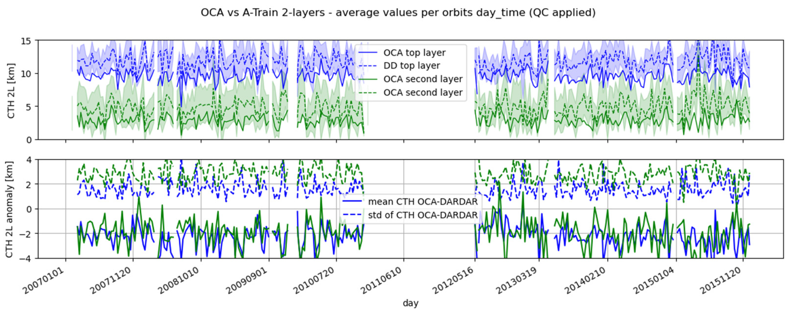
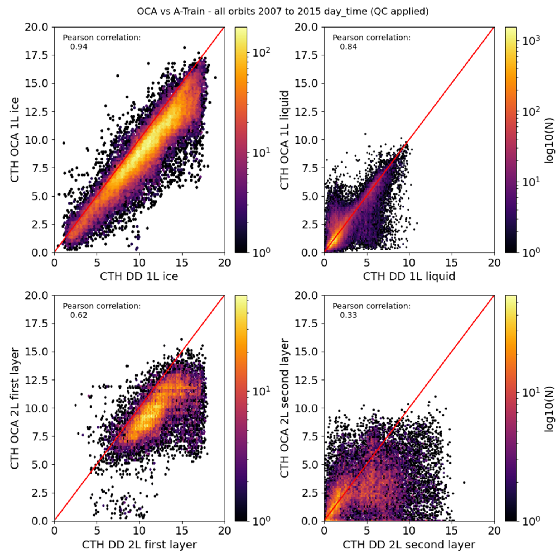
5.1.1. Cloud-Top Height

For single-layer profiles, the time series of the retrieved cloud-top height by OCA against the cloud-top height estimated from DARDAR (Figure 8) is consistent through the analyzed period and shows that on average, OCA cloud tops are 1.7 km lower than those in DARDAR for ice clouds and 0.1 km lower for liquid clouds.

This result is consistent with earlier results (e.g., [3,30,31]) and highlights the discrepancy in the sensitivity to the effective top layer by the radiometric passive measurements used by OCA and the direct backscatter measured by the lidar. The difference between the two measurements is larger for high ice clouds because they (often) have low density and therefore extinction, permitting radiation to originate from deeper in the cloud. This inherent characteristic of the passive measurements is not accounted for in the OCA fast forward model: a set of lookup tables describe the cloud layers as plane-parallel with an effectively infinitesimal geometrical thickness. Therefore, the retrieved cloud-top height will be placed at the level of the effective emission of the cloud because no extra information about the vertical profile of the cloud properties is provided to the forward model. The OCA algorithm can benefit from the use of an updated cloud model based on a set of climatological cloud profiles derived from CALIPSO and CloudSat measurements [30]. The use of a more complex, vertically inhomogeneous cloud model significantly impacts the retrieval of cloud-top height for high ice clouds and has been found to reduce the difference with respect to the cloud-top height estimated from lidar/radar measurements.

Results for the cloud-top height retrieval for two-layer clouds shows results comparable to the single layer pixel for the upper layer, but with larger differences (2.0 km lower for OCA), while the second layer is in general 1.9 km lower in OCA compared to DARDAR.

The number of two-layer pixels within the total dataset of collocated and synchronized A-Train and OCA retrievals is about 25%. For these pixels, we only analyzed those where both OCA and DARDAR report a multi-layer situation. The smaller sample explains the larger dispersion shown in Figure 9. Although, as discussed in Section 4.2, we added the estimate of the upper-layer COT to increase the confidence in the multi-layer classification, situations where the optical thickness of the topmost layer is at the limit of what OCA is capable to observe are still possible. In some cases, this results in OCA more effectively measuring the height of underlying cloud layers rather than of the overlying thin ice cloud layer.

The results for all pixels analyzed over the period 2007–2015 are summarized in the aggregated scatter plots of Figure 10. In line with Figure 8, it can be seen that in single-layer situations, OCA compares well with DARDAR for mid- and low-level clouds, especially for the liquid category, and that the bias increases for high ice clouds. In line with Figure 9, in the two-layer cases, the bias for the topmost layer is similar to that of high single-layer clouds but with larger dispersion. The comparison for the cloud height in the second layer shows significant dispersion and a high frequency of clouds placed too low by OCA. For some of these points, the DARDAR identification of the overlapping layers does not match the same layers sensed by OCA, possibly because of a very thin upper layer.

Nighttime orbits cover a shorter period, but the general result for the CTH comparison is similar to that of the daytime orbits, however with a larger dispersion and slightly larger mean differences (

Table 3. Summary of the statistics from a set of A-Train granules collocated with SEVIRI pixels. Cloud-top height (CTH), ice cloud effective radius at cloud top (CRE), and ice cloud optical thickness (COT) are shown for OCA and DARDAR retrievals. In brackets, the standard deviation computed over all the collocated pixels.

	OCA		DARDAR		OCA-DARDAR
	Day (2007–2016)	Night (2007–2010)	Day (2007–2016)	Night (2007–2010)	Day (2007–2016)	Night (2007–2010)
CTH (km)	Mean (std)	Mean (std)	Mean (std)	Mean (std)	Mean (std)	mean (std)
Ice, single	9.2 (3.0)	8.2 (3.2)	10.8 (3.3)	10.2 (3.7)	−1.6 (1.2)	−2.0 (1.6)
Liquid, single	1.9 (1.5)	1.7 (1.3)	2.0 (1.6)	1.8 (1.4)	−0.1 (0.9)	−0.1 (0.8)
Two-layer upper	9.7 (1.8)	9.8 (1.7)	12.1 (2.4)	12.7 (2.6)	−2.4 (1.9)	−2.9 (2.0)
Two-layer lower	2.9 (2.0)	2.6 (2.1)	4.9 (3.2)	5.0 (3.3)	−2.0 (3.1)	−2.3 (3.3)
CRE (μm)
Ice, single	30.8 (12.9)	50.9 (16.3)	32.9 (8.9)	32.7 (11.2)	−2.1 (15.9)	18.4 (19.2)
Two-layer upper	17.4 (6.1)	16.5 (4.9)	29.3 (5.8)	26.0 (6.6)	−11.9 (7.9)	−9.4 (7.2)
Log10 (COT)
Ice, single	0.87 (0.64)	1.01 (0.40)	0.78 (0.63)	0.91 (0.64)	0.08 (0.44)	0.18 (0.65)
Two-layer	0.87 (0.65)	0.70 (0.27)	0.42 (0.50)	0.35 (0.42)	0.44 (0.52)	0.35 (0.45)

).

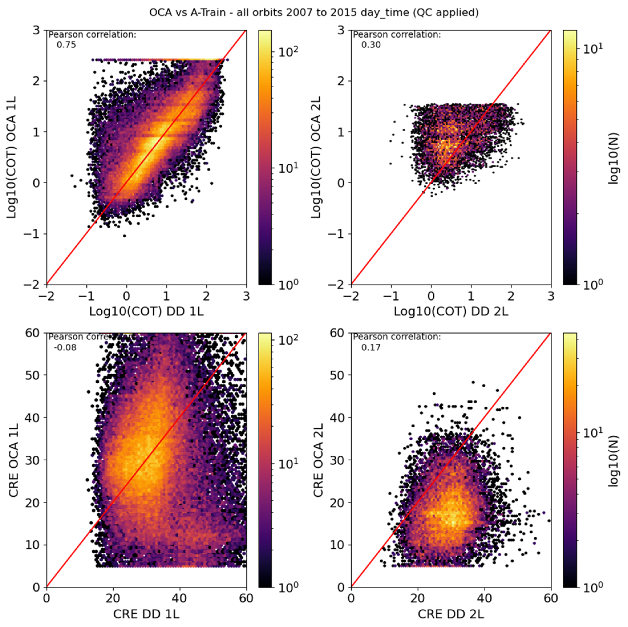
5.1.2. Ice Cloud Optical Thickness and Effective Radius

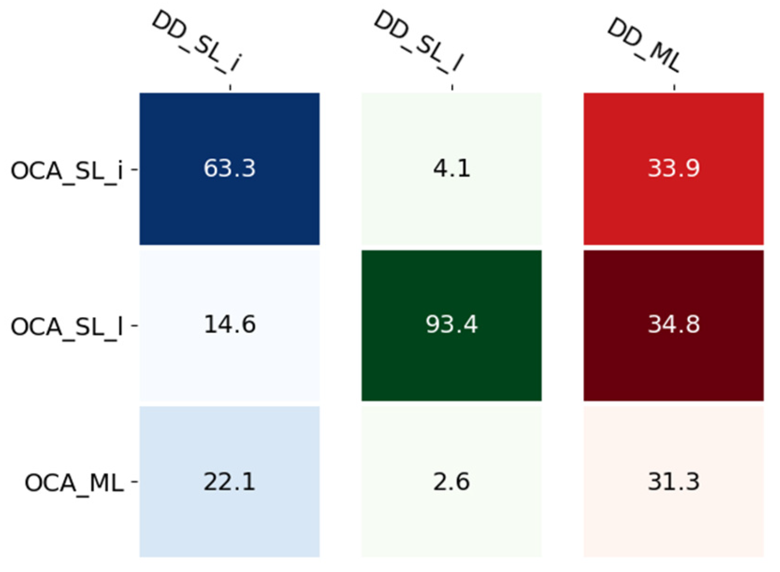
The comparison of the retrieved cloud optical thicknesses for ice clouds only reveals good agreement for the single-layer cases (Figure 11, upper panels). This is true especially for the daytime retrieval, which benefits from the availability of short-wave channels to constrain the total optical thickness. During nighttime, the retrieved values are less accurate. The nighttime optical thickness retrievals are exclusively based on SEVIRI’s thermal channels, which can provide useful information only up to an optical thickness of about 5. The emission of clouds with an optical thickness higher than 5 is saturated, resulting in an effectively unconstrained retrieval and larger uncertainty.

For two-layer cases, the comparison is complicated by the fact that the overlapping layers are often of ice type over liquid water clouds (about 60% of all multi-layer cases on average). In these cases, the retrieved optical thickness from OCA will be higher than those from DARDAR, for which no information is available for the liquid cloud layers. Therefore, we restricted the comparison to cases where both layers in DARDAR were detected as ice. This, however, does not always guarantee complete consistency in the cloud types along the full profile, as it is possible that in certain conditions, the presence of residual liquid or mixed-phase clouds is not correctly identified in the lidar/radar classification.

The comparison of OCA and DARDAR particle size (Figure 11, lower panels) reveals significant dispersion, with OCA spanning a large range of particle sizes from 5 μm and up to 60 μm (the upper boundary of the lookup tables used in the forward model). The values retrieved by DARDAR cover a smaller range of particle sizes, with values between 15 μm and 50 μm. This discrepancy is partly related to the effective cloud level measured by the instruments, the real vertical gradient in particle size distribution within the cloud, and the ice crystal model and size distributions assumed in both retrievals. Daytime retrievals from OCA are constrained by the solar channels, while at nighttime, the OCA retrievals show no skill and are almost uncorrelated with the particle sizes retrieved by DARDAR.

In two-layer conditions, OCA retrieves the particle size of the upper layer using thermal channels only. For these conditions, the upper layer is generally thin enough to allow for retrievals with some skill and smaller retrieval error and data dispersion. The particle size retrieval shows large differences, as it is not constrained by measurements in the solar channels.

5.1.3. Cloud Phase

The cloud feature mask includes information about the phase of cloud layers, and thus the collocated and synchronized OCA and DARDAR retrievals can also be used for validating the cloud phase estimate from OCA.

From the results summarized in Figure 12, we can see that of all OCA retrievals in the single-layer ice cloud category (blue column), 63% fully agrees with DARDAR (categories OCA_SL_i and DD_SL_i), 22% partly agrees with DADAR falling in the two-layer category (OCA_ML vs. DD_SL_i), and ~15% disagrees with DARDAR and retrieves single-layer liquid clouds (OCA_SL_l). For the single-layer liquid category (green column) there is a very high agreement of about 93% (OCA_SL_l vs. DD_SL_l).

In OCA, the two-layer category always assigns the phase ice to the upper layer and the phase undetermined to the lower layer. We used DARDAR to analyze the phase of the upper and lower layer. The results show that in most cases (95%), the upper layer is of ice phase and the lower layer has a slight prevalence (55%) of liquid water phase. In terms of detection of multi-layer situations, the comparison shows that OCA and DARDAR agree in about a third of the cases (OCA_ML vs. DD_ML). The remaining two-thirds of multi-layer cases are assigned by OCA either as single-layer ice or as single-layer liquid clouds. Results are shown here for the daytime orbits but the same also applies to the nighttime orbits, without appreciable differences.

On one hand, these results depend on the definition of the reference truth for multi-layered cloud profiles, which is not always clear-cut, in particular for thin upper cloud layers. In this case, the CTH retrieved by OCA often tends to be closer to the second layer in the DARDAR profile, or between the two layers when both cloud layers have a significant impact on the upwelling radiance. This disagreement in categorization between OCA and DARDAR was observed in about 14% of all OCA ice cloud types.

On the other hand, when OCA retrieves a single-layer ice cloud as multi-layer, differences in the retrieved CTH are smaller and results are similar to what was already analyzed in Figure 12. This latter case happens in about 17% of all OCA ice cases, often when the upper cloud layer has low particle density or a challenging vertical distribution of ice water content.

In general, including the pixels where the OCA multi-layer categorization does not match DARDAR in the CTH evaluation, scores suffer a slight degradation. This is relevant to correctly interpret the comparisons based on disk-averaged values in OCA including all cloud types.

5.1.4. Evaluation of the Quality of the OCA Product Uncertainty

The optimal estimation algorithm at the core of the OCA retrieval allows for the computation of an uncertainty estimate for each state variable and, as mentioned before, these error estimates are used to provide basic quality control for the products to remove the retrievals with large uncertainty.

An estimate of retrieval uncertainty is valuable for a CDR, but the task is generally not straightforward. A series of different contributions affect such an analysis from the uncertainty in the reference dataset to the errors related to the collocation procedure, the geophysical variability of the variable being analyzed, and the differences in the physical quantity measured in the two comparing datasets [32]. A full evaluation of the quality of OCA uncertainty for all variables is outside the scope of this work and we provide here the results of an estimate of the accuracy of the cloud-top height uncertainty only. For the details of the approach used in the analysis, we refer the reader to [28].

The quality of OCA CTH uncertainty is evaluated using the difference between the OCA and DARDAR CTH (x_oca − x_dd) as a metric, scaled by an estimate of the total uncertainty. Assuming negligible uncertainty in the CTH retrieved by CloudSat/CALIPSO, the total uncertainty depends on two contributions, the OCA retrieval uncertainty (u_oca) and the uncertainty arising from the comparison procedure (u_comp) including the spatiotemporal mismatch in the collocation, difference in the measurements from active and passive instruments, and assumptions used in the definition of cloud-phase and multi-layer situations. The metric is therefore defined as the ratio $x_{oca}-x_{dd}/\sqrt{u_{oca}^2+u_{comp}^2}$, and it shows how the total uncertainty compares to the difference between the OCA CTH and the reference values from DARDAR.

Using this approach, we find that for both the nighttime and daytime one-layer CTH, the uncertainty is a factor between 8 and 15 too small. A reason for this result is the known underestimation of the uncertainty contribution coming from the characterization of scene and cloud properties in the OCA forward model. Another reason is the choice of the error assigned to the prior values, which follows the Twomey–Tikhonov approach of imposing minimal external constraints on the retrieval. If this choice on one hand preserves a high precision in the CTH retrieval, on the other hand, it results in a final retrieval uncertainty not fully representative of the true uncertainty [33].

An inflation by a factor of about 10 in CTH uncertainty provided in this CDR is therefore suggested as the accuracy of the product. The precision is certainly higher, and this should be considered depending on the specific application.

The uncertainty computed for the other variables should likely be inflated to a similar degree, but a full evaluation is not attempted for this first version of the data record.

5.2. Comparison against MODIS L3, CLAAS-3, and CALIPSO L3 Products

This section presents the comparison of OCA CDR against the cloud products from the MODIS and CLAAS-3 CDRs, i.e., cloud-top pressure, cloud particle effective radius, and cloud optical thickness. All MODIS products used in the following comparisons are the average between the AQUA and the TERRA retrievals. This is a cross-comparison between retrievals based on passive imager measurements and therefore shall be considered as an evaluation of the consistency in the scientific content of OCA CDR and not as its validation, which is rather intended against products obtained from independent measurements. Spatial maps are provided for one seasonal average (winter defined as the mean between December through February) but results are similar for other times of the year.

With the pre-processing applied to the data described in Section 4.2, we reduced, as much as possible, the differences in the three datasets caused by the differences in time averaging, spatial gridding, and type/phase aggregation.

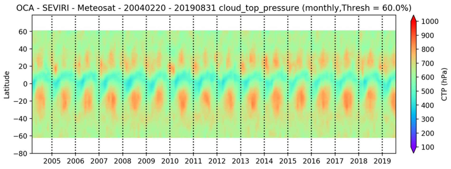
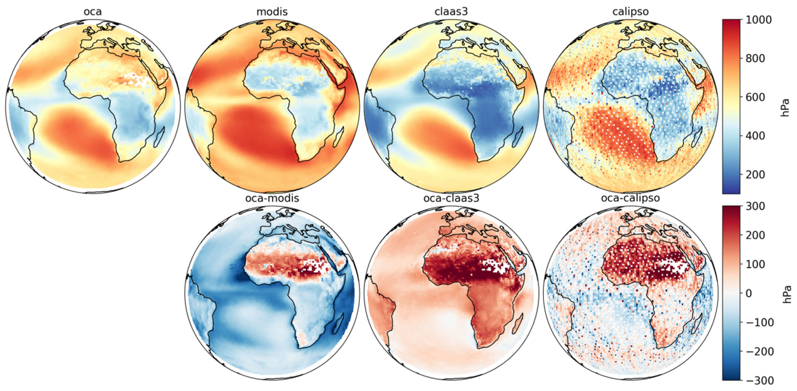
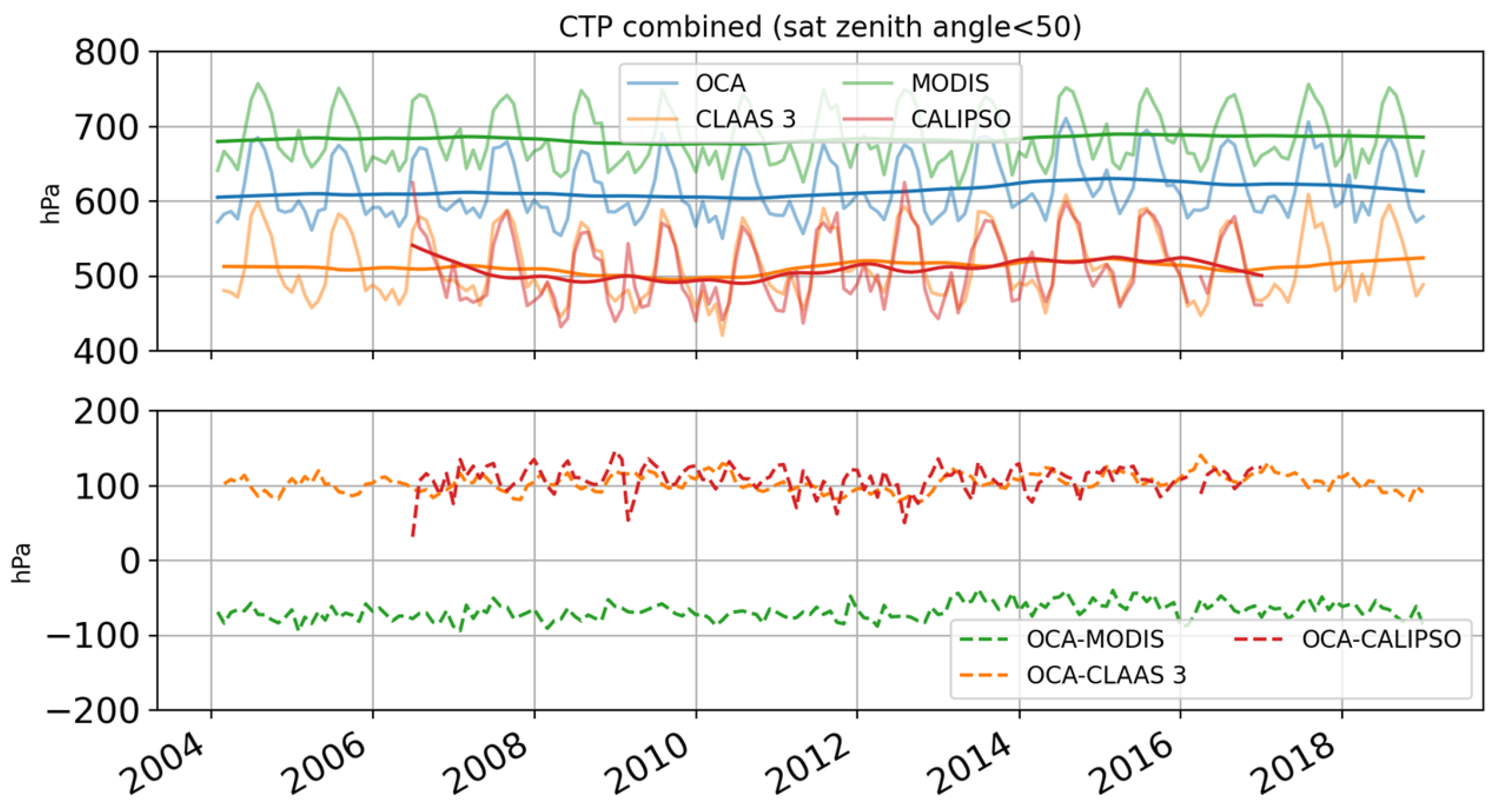
5.2.1. Cloud-Top Pressure (CTP)

The OCA mean spatial distribution of CTPs captures the large-scale seasonal features in cloud height and is comparable with the other datasets (Figure 13), but with distinct differences. On average, the OCA CTP falls between those retrieved by MODIS and CLAAS-3, since the latter is trained to closely match the CTP retrieved by CALIPSO [22]. Generally, OCA retrieves lower CTPs than MODIS over land and water and higher CTPs than CLAAS-3, with larger differences over land.

In agreement with the analysis against CloudSat and CALIPSO data in Section 5.1, the differences are smallest in areas dominated by thick low water clouds, such as the stratocumulus region over the SE Atlantic. The observed differences are largest over the intertropical convergence zone, where a larger fraction of ice and multi-layer clouds exists.

In two-layer cases, the CTP retrieved by MODIS under the assumption of single-layer conditions will provide a CTP between the lowest and highest of the cloud layers while OCA is able to get closer to the topmost of the overlapping layer, as discussed in Section 5.1.1.

OCA CTP compares relatively good against the “passive” flavor of the CALIPSO GEWEX, which is intended to provide values closer to the cloud top detected by a passive instrument.

A distinct feature in the OCA dataset is the large occurrence of high CTPs (low cloud tops) over the Sahara Desert. This problem is caused by contamination of surface signal over very bright and hot surfaces that is transmitted through high thin ice clouds, which leads to an overestimation of CTP over the desert. The feature is further enhanced in the OCA data due to the very cloudy sky-conservative cloud mask used in input. This means that the algorithm tries to process a lot of pixels with very thin cloud layers. As OCA CDR includes the cloud probability fractions, the user can filter out areas with very thin clouds.

The time series of the area-weighted disk average CTPs over the whole period 2004–2019 (Figure 14) confirms the mean differences between the datasets. OCA sits in between the MODIS and CLAAS-3 retrievals. The CALIPSO L3 GEWEX time series covers a shorter time frame than the other three and shows on average lower CTP than OCA, part of the difference being dominated by the positive bias shown by OCA over North Africa. When the CALIPSO L3 values not adjusted to represent passive imager retrievals are used, differences against both OCA and MODIS increase substantially while showing remarkable agreement with CLAAS-3, whose algorithm is indeed trained to represent CALIOP measurements (Figure 15). The four time series are consistent and highly correlated, showing the same features throughout the years.

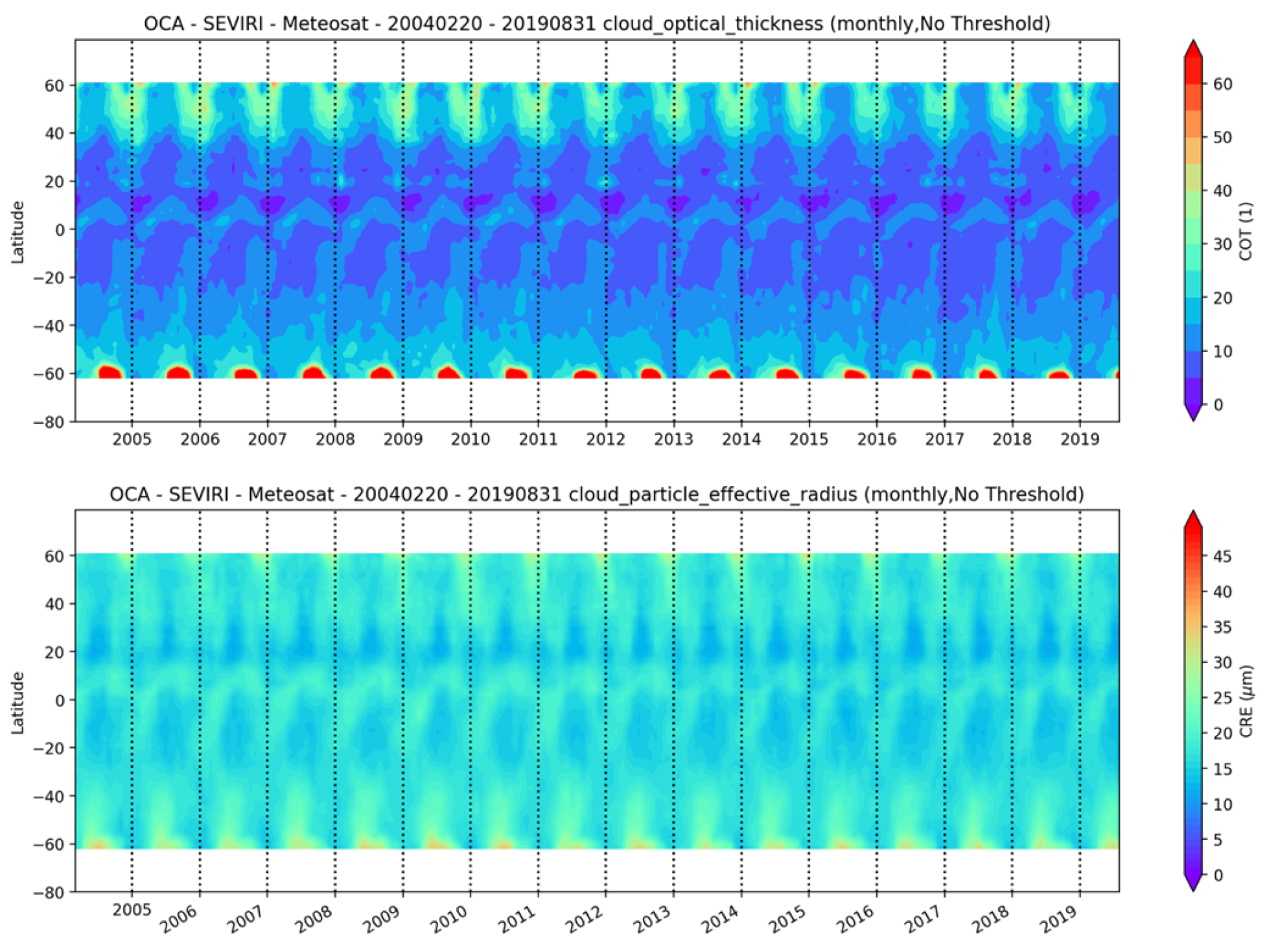
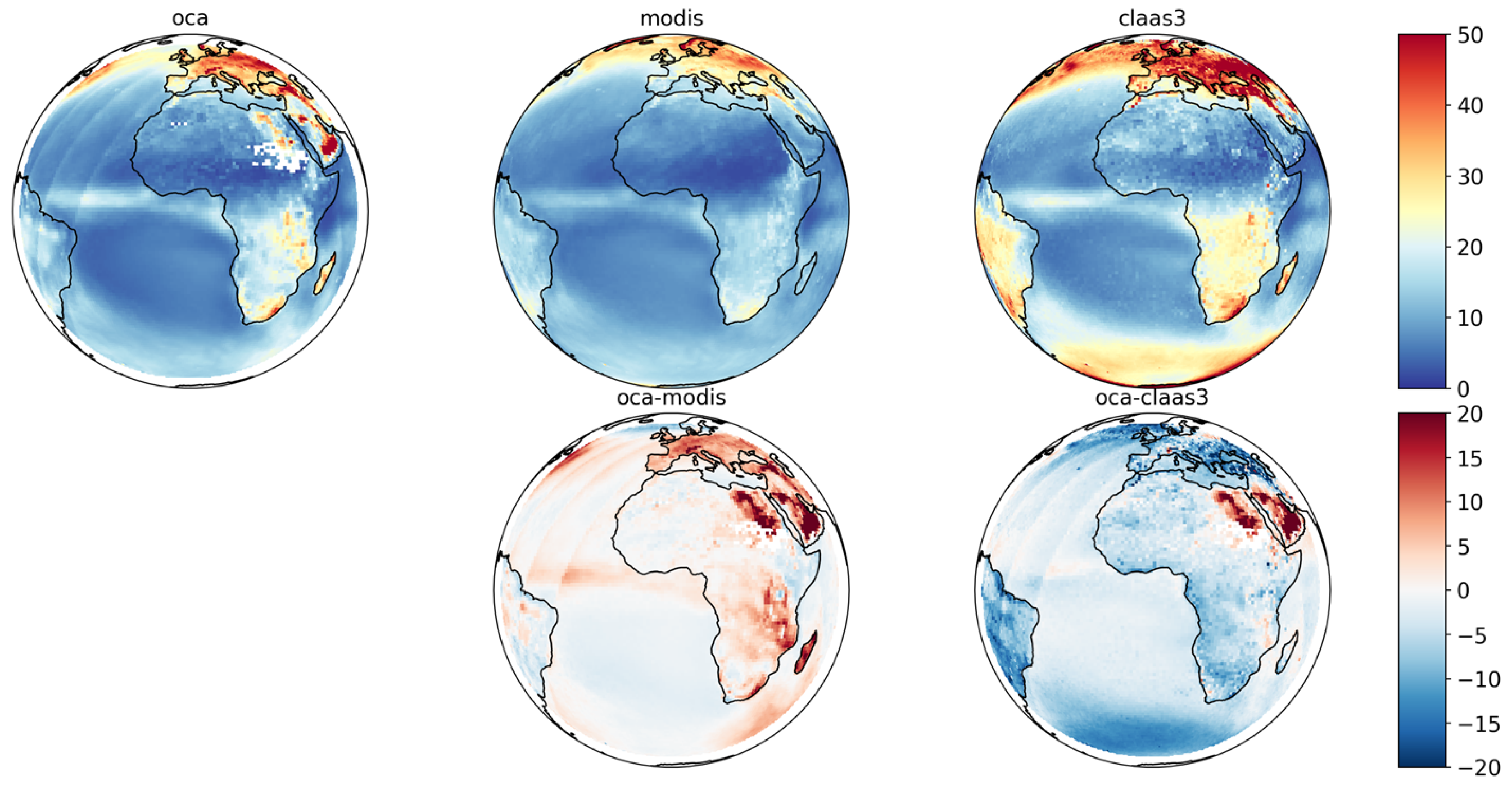
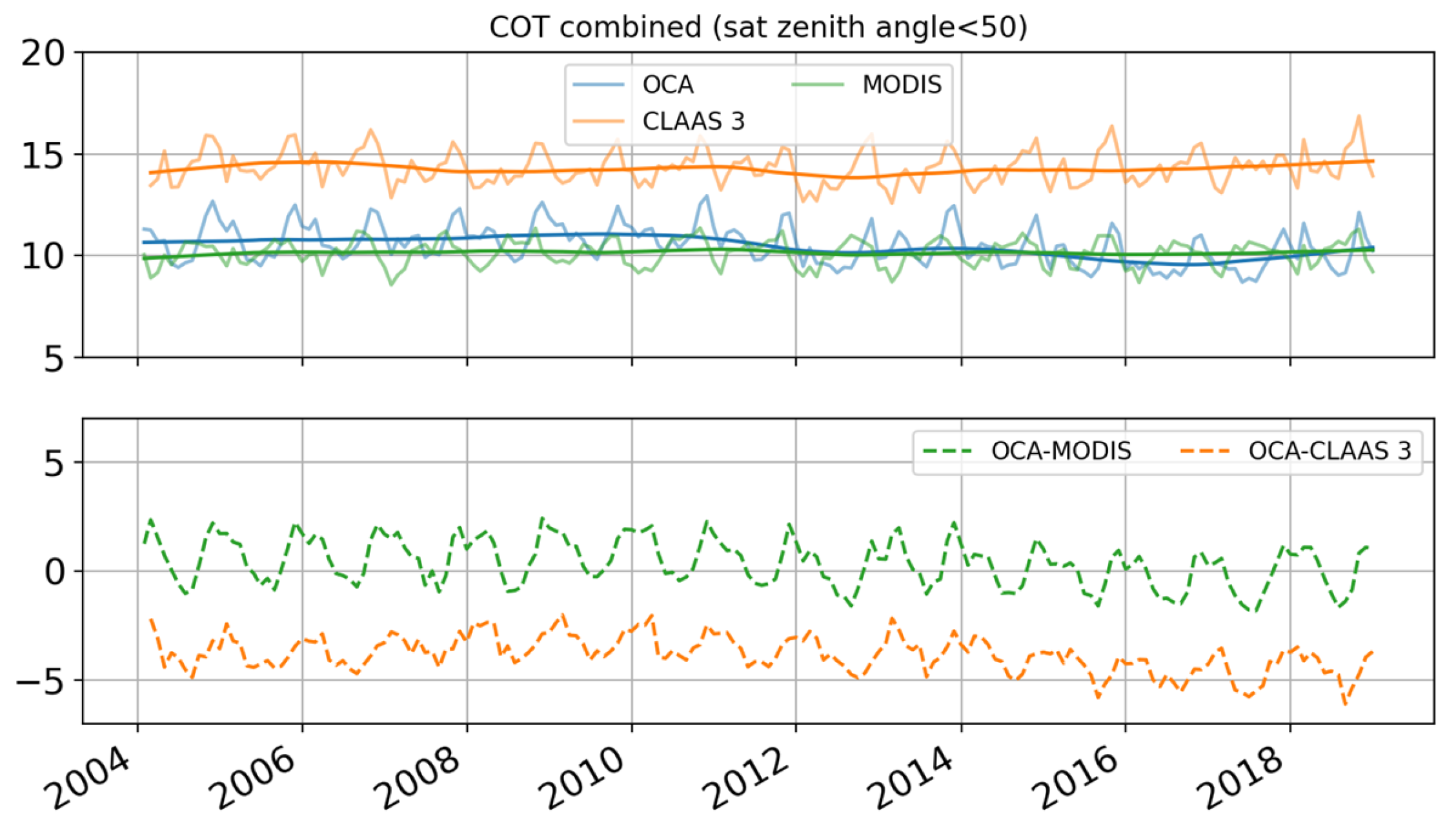
5.2.2. Cloud Optical Thickness (COT)

The spatial distribution of OCA total cloud optical thickness, combining ice, liquid, and multi-layer cloud types, is in general agreement with the other two datasets, although there are some distinct differences (Figure 16). OCA retrieves larger COTs than MODIS over land in Central Africa, while it retrieves generally lower values than CLAAS-3 over land and sea, particularly over the Southern Ocean. Large positive COT anomalies in OCA are found in combination with large solar zenith angles and large viewing zenith angles. In these situations, most of the signal in the solar channels comes from backscattered radiation, often from the side of the clouds, and the illumination and view angles of the cloud are much lower than the plane-parallel assumption in the forward model is able to correctly model. A similar effect is seen in the CLAAS-3 record, but here, the effect is smaller because the CLAAS-3 L2 products used in the generation of the L3 dataset are limited to a solar zenith angle <75°. Although we created the monthly averages trying to minimize their impact, OCA retrievals in the twilight are partly included in the monthly means generation (Section 3.2).

Areas of large positive anomalies over the eastern Sahara and Arabian Peninsula are caused by pixels defined as cloudy that are in reality surface features misinterpreted by the cloud mask, as discussed for the CTP in Section 5.2.1. In this situation, OCA COT retrieval is not reliable. These pixels can be filtered by applying a higher cloud probability threshold to the product.

The time series of the retrieved COT over the full period shows that the OCA COT is closer to the MODIS COT and lower than that in CLAAS-3, with a distinct annual cycle and a maximum around December (Figure 17).

From about the end 2012, the OCA time series shows a subtle yet systematic decrease in the mean COT (from 10.8 pre 2012 to 10.0). It is possible that this change is related to issues in the short-wave channel calibration of SEVIRI. The OCA CDR uses the operationally calibrated Level 1 data that were adjusted with a set of (static) offsets to account for the significant deviations found in comparisons between SEVIRI and MODIS Level 1 data [11]. This static correction is likely to have left some uncorrected drifts and jumps in the accuracy of the calibration, especially at the interchanges between instruments.

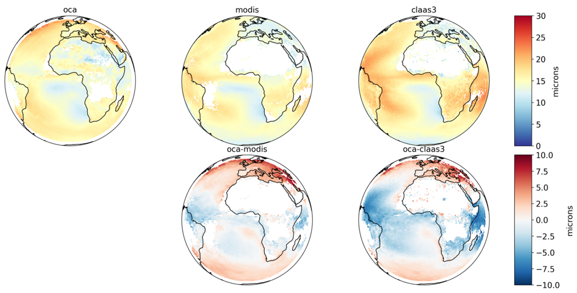
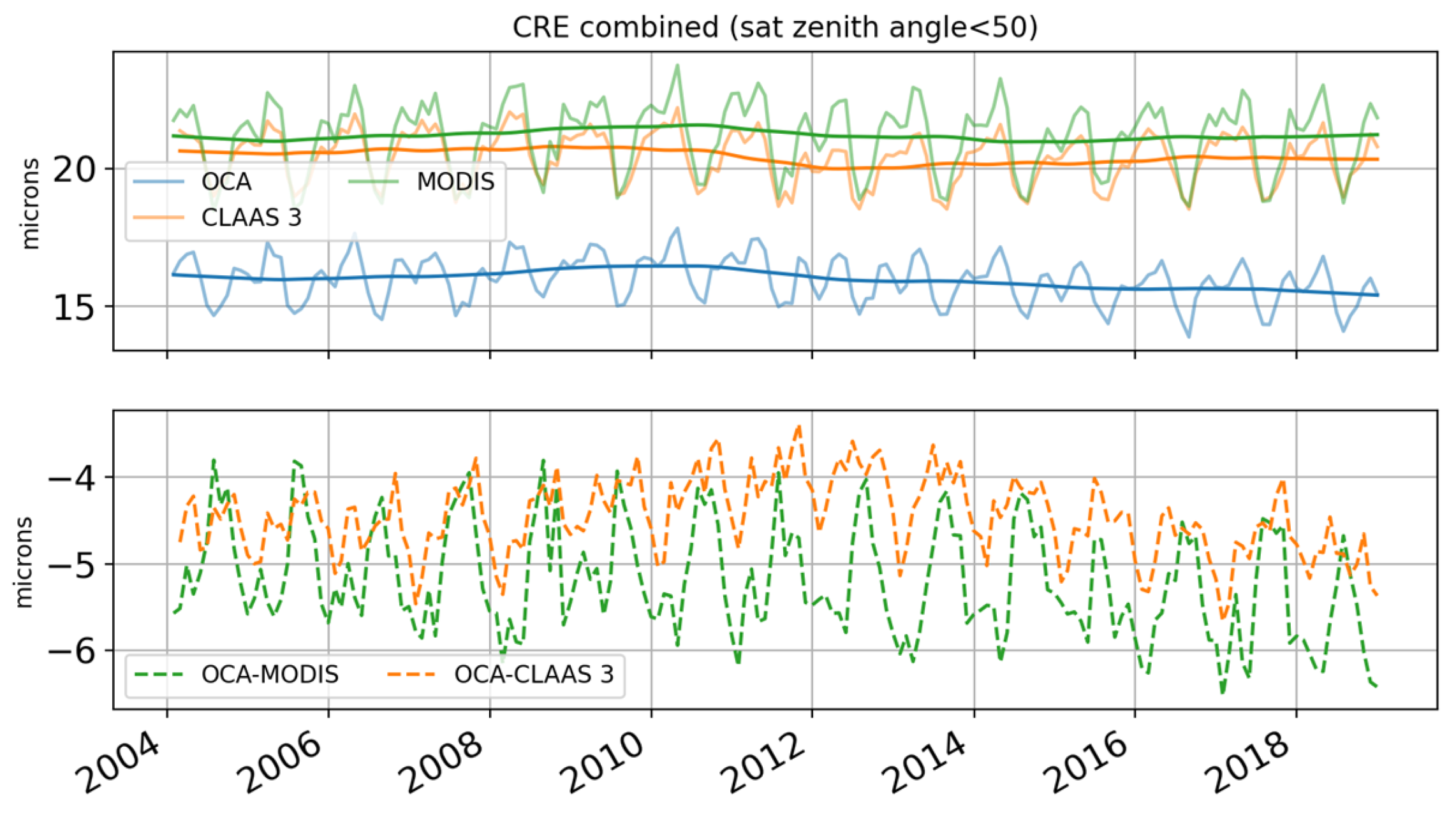
5.2.3. Cloud Particle Effective Radius (CRE)

The analysis of the cloud particles’ effective radii was determined for combined ice and liquid phase. To be consistent with the combined phase in OCA, the CRE for liquid and ice clouds in the other two datasets were combined, weighted by the respective ice and liquid fraction. The seasonally averaged cloud particle sizes for the three datasets are shown in Figure 18. All three datasets use the same underlying ice crystal model, represented by aggregates of severely roughened solid columns (based on [7,34,35]).

OCA retrieves, on average, the lowest values, especially in areas with high ice and two-layer cloud frequency. This underestimation is the result of the combination of few factors:

(1)

The maximum limit allowed for in the retrieval of CRE for liquid clouds is set at 23 μm for OCA, while for CLAAS-3 and MODIS L3, it is allowed to retrieve liquid droplets up to 30 μm. This choice mostly affects the trade cumulus areas over the Equatorial and Tropical Atlantic Ocean, as observed in Figure 19, where areas with a fraction of single-layer liquid clouds in OCA larger than 60% are compared to the liquid CRE in MODIS and CLAAS-3 datasets. In areas where the phase fraction in the monthly averages includes both liquid and ice clouds, the smaller CRE in these areas will contribute to a smaller average CRE in OCA. The maximum CRE limit in OCA will be revised in a future version of this CDR.

(2)

As discussed in Section 5.1.2, in comparison with DARDAR, the OCA CRE retrieval for the upper layer in two-layer cases is biased low. This is due to the lack of constraint from the solar channels, which are currently not used for two-layer retrieval. This limitation will also be addressed in the next CDR, with a new forward model capable of providing consistent results between single- and two-layer situations.

(3)

The already mentioned too-large quantity of low liquid clouds over North Africa with small liquid droplets.

The time series of the retrieved particle size (Figure 20) shows that the differences between the three datasets are stable throughout the period, although the OCA time series shows a slight change from about 2012, as observed for the COT.

6. Discussion and Limitations

This first release of the OCA CDR provides a coherent dataset of cloud properties including overlapping cloud layers using SEVIRI measurements. The user of this dataset should consider the following limitations, which we plan to address in a subsequent release:

As evidenced by the comparison against independent retrieval products, the quality of COT and CRE retrievals changes significantly between daytime and nighttime periods. This is expected, given that a strong constraint for these quantities is given by the solar channels. Although we chose to provide the product for all SEVIRI repeat cycles, users should be aware of the lower quality of nighttime retrievals. This difference does not apply to CTP retrieval, as this mostly depends on infrared channels.

Cloud retrieval over bright surfaces like deserts is often of low quality: for COT, a combination of imperfect cloud screening giving false detections and poor constraints on COT at night leads to anomalously high values. Moreover, anomalously high CTP values over bright surfaces, especially for high thin clouds, are the result of a weakly constrained situation highly sensitive to the definition of the first-guess CTP, currently not optimal in these conditions. However, for the current CDR, as a mitigation measure, the input cloud mask array is included in the product so that any user can decide for further pixel screening depending on the application.

Like other retrievals based on passive imagers, OCA CTPs are generally higher (lower altitude) than observed CTPs as sensed by satellite or airborne lidars. Maximum differences (~1.5 km) are found for high thin ice clouds. As explained in Section 5.1.1, this is due to the current design of the retrieval algorithm, whose cloud model is represented by a homogeneous, infinitesimally thin plane-parallel layer. This means that effects due to the vertical structure of clouds, horizonal inhomogeneity, and three-dimensional photon transport are not considered. Therefore, the retrieved cloud properties will be representative of the level of the effective emission of the cloud for infrared channels, or effective photon penetration depth for solar channels, because no extra information about the vertical profile of the cloud properties is provided to the forward model. Tests with a prototype version of the OCA algorithm have shown that the use of an updated cloud model based on a set of climatological cloud profiles from CALIPSO and CloudSat measurements is capable of providing information on the vertical distribution of properties, bringing the estimated cloud top close to what is observed by the lidar.

Finally, the retrieval of overlapping cloud layers is currently performed with a simplified forward model that does not directly use information from the solar channels [3]. The second layer is effectively represented as an elevated surface, with the temperature representative of the cloud top of the lower layer. The use of this simplified model improves the retrieval of the CTP of the upper layer but with lower accuracy for the retrieval of COT and CRE, lacking the constraint provided by the solar channels. The current revised OCA prototype overcomes this shortcoming by employing a more complete forward model capable of simulating the full short-wave and long-wave radiative transfer between the cloud layers.

7. Conclusions

The CDR and archived near-real-time OCA products are consistent and in close agreement, especially for the CTP parameter, with some differences due to the usage of different input data for the retrieval (for details, see [28]). The cloud mask used in the CDR has a larger amount of thin cirrus for which the reliability of OCA retrieval is low. The cloud mask is included in the data files so that users can filter out products based on different cloud probability thresholds and the specific application. The CDR uses the ECMWF ERA-Interim meteorological reanalysis profiles while the NRT uses ECMWF operational model forecasts. Those model data are used in the CDR at a higher vertical resolution than for the generation of the NRT products, and this especially has an impact on the definition of cloud-top height close to temperature inversions.

The CDR is consistent with measurements and retrieval products from CloudSat and CALIPSO collocated with SEVIRI pixels over the period 2007–2015. The biases in the OCA products, already known from previous studies, have been confirmed. In particular, when the reference cloud-top height is defined by lidar measurements, radiometer-based cloud-top height retrievals like OCA tend to be biased low, especially for high thin ice clouds (~1.5 km below the real top). The cloud-top height retrieval for overlapping cloud layers shows larger biases than for single-layer clouds but improves with respect to algorithms that only assume single-layer clouds. The retrieval of COT and CRE is most reliable for daytime measurements, while CTP is of comparable quality for daytime and nighttime SEVIRI slots. The current two-layer algorithm is restricted to use of infrared channels, and these retrievals therefore suffer from the lack of solar channel input. A more complete and robust two-layer forward model has been implemented in the current OCA prototype and will be used for the next version of this CDR.

The comparison of the OCA CDR against other two independent satellite reference CDRs (MODIS L3 and CLAAS-3) shows that the products of the three independent CDRs are compatible and consistent over the whole 2004–2019 period. However, they show differences linked to the different algorithms and cloud model assumptions. Cloud ice particle size shows the largest disagreement, especially when OCA detects two-layer situations. OCA shows a trend for the COT and CRE time series from roughly 2012 not observed in the other two CDRs. A possible cause of this is the use of constant calibration coefficients for short-wave channels in the creation of this CDR. These will be replaced by an updated set of time-varying coefficients based on new vicarious calibration at EUMETSAT in the new version of this CDR.

References

1. Forster, P.; Storelvmo, T. The Earth’s Energy Budget, Climate Feedbacks, and Climate Sensitivity. In Climate Change 2021: The Physical Science Basis. Contribution of Working Group I to the Sixth Assessment Report of the Intergovernmental Panel on Climate Change; Cambridge University Press: Cambridge, UK; New York, NY, USA, 2021; pp. 923–1054. [Google Scholar] [CrossRef]
2. Schmetz, J.; Pili, P.; Tjemkes, S.; Just, D.; Kerkmann, J.; Rota, S.; Ratier, A. Supplement to An Introduction to Meteosat Second Generation (MSG): SEVIRI CALIBRATION. Bull. Amer. Meteor. Soc. 2002, 83, 992. [Google Scholar] [CrossRef]
3. Watts, P.D.; Bennartz, R.; Fell, F. Retrieval of two-layer cloud properties from multispectral observations using optimal estimation. J. Geophys. Res. 2011, 116, D16203. [Google Scholar] [CrossRef]
4. Stöckli, R.; Duguay-Tetzlaff, A.; Bojanowski, J.; Hollmann, R.; Fuchs, P.; Werscheck, M. CM SAF ClOud Fractional Cover Dataset from METeosat First and Second Generation, 1st ed.; (COMET) Satellite Application Facility for Climate Monitoring; EUMETSAT: Darmstadt, Germany, 2017. [Google Scholar]
5. EUMETSAT. MTG-FCI: ATBD for Optimal Cloud Analysis Product. 2016. Available online: https://www-cdn.eumetsat.int/files/2020-06/pdf_mtg_atbd_oca.pdf (accessed on 2 August 2024).
6. Poulsen, C.A.; Siddans, R.; Thomas, G.E.; Sayer, A.M.; Grainger, R.G.; Campmany, E.; Dean, S.M.; Arnold, C.; Watts, P.D. Cloud retrievals from satellite data using optimal estimation: Evaluation and application to ATSR. Atmos. Meas. Tech. 2012, 5, 1889–1910. [Google Scholar] [CrossRef]
7. Baum, B.A.; Yang, P.; Heymsfield, A.J.; Bansemer, A.; Cole, B.H.; Merrelli, A.; Schmitt, C.; Wang, C. Ice cloud single-scattering property models with the full phase matrix at wavelengths from 0.2 to 100 µm. J. Quant. Spectrosc. Radiat. Transf. 2014, 146, 123–139. [Google Scholar] [CrossRef]
8. Hocking, J.; Rayer, P.; Rundle, D.; Saunders, R. RTTOV v11 Users Guide. NWP SAF, EUMETSAT. 2015. Available online: https://nwp-saf.eumetsat.int/site/download/documentation/rtm/docs_rttov11/users_guide_11_v1.4.pdf (accessed on 2 August 2024).
9. Stamnes, K.; Tsay, S.-C.; Wiscombe, W.; Jayaweera, K. Numerically stable algorithm for discrete-ordinate-method radiative transfer in multiple scattering and emitting layered media. Appl. Opt. 1988, 27, 2502. [Google Scholar] [CrossRef]
10. Laszlo, I.; Stamnes, K.; Wiscombe, W.J.; Tsay, S.-C. The Discrete Ordinate Algorithm, DISORT for Radiative Transfer. In Light Scattering Reviews; Kokhanovsky, A., Ed.; Springer: Berlin/Heidelberg, Germany, 2016; Volume 11, pp. 3–65. [Google Scholar] [CrossRef]
11. Meirink, J.F.; Roebeling, R.A.; Stammes, P. Inter-calibration of polar imager solar channels using SEVIRI. Atmos. Meas. Tech. 2013, 6, 2495–2508. [Google Scholar] [CrossRef]
12. Dee, D.P.; Uppala, S.M.; Simmons, A.J.; Berrisford, P.; Poli, P.; Kobayashi, S.; Andrae, U.; Balmaseda, M.A.; Balsamo, G.; Bauer, P.; et al. The ERA-Interim reanalysis: Configuration and performance of the data assimilation system. Quart J. Royal Meteoro. Soc. 2011, 137, 553–597. [Google Scholar] [CrossRef]
13. EUMETSAT. Clear Sky Reflectance Map: Product Guide. 29 May 2015. Available online: https://user.eumetsat.int/s3/eup-strapi-media/pdf_crm_factsheet_e44562ba08.pdf (accessed on 2 August 2024).
14. EUMETSAT. Optimal Cloud Analysis (OCA) Release 1 Product Users Guide. 2021. Available online: https://user.eumetsat.int/s3/eup-strapi-media/Optimal_Cloud_Analysis_OCA_Release_1_Product_Users_Guide_5120a10382.pdf (accessed on 2 August 2024).
15. Delanoë, J.; Hogan, R.J. A variational scheme for retrieving ice cloud properties from combined radar, lidar, and infrared radiometer. J. Geophys. Res. 2008, 113, D07204. [Google Scholar] [CrossRef]
16. Delanoë, J.; Hogan, R.J. Combined CloudSat-CALIPSO-MODIS retrievals of the properties of ice clouds. J. Geophys. Res. 2010, 115, D00H29. [Google Scholar] [CrossRef]
17. Winker, D.M.; Pelon, J.R.; McCormick, M.P. The CALIPSO mission: Spaceborne lidar for observation of aerosols and clouds. In Proceedings of the Third International Asia-Pacific Environmental Remote Sensing Remote Sensing of the Atmosphere, Ocean, Environment, and Space, Hangzhou, China, 23–27 October 2002; Singh, U.N., Itabe, T., Liu, Z., Eds.; SPIE: San Francisco, CA, USA, 2003; p. 1. [Google Scholar] [CrossRef]
18. Stephens, G.L.; Vane, D.G.; Boain, R.J.; Mace, G.G.; Sassen, K.; Wang, Z.; Illingworth, A.J.; O’Connor, E.J.; Rossow, W.B.; Durden, S.L.; et al. THE CLOUDSAT MISSION AND THE A-TRAIN: A New Dimension of Space-Based Observations of Clouds and Precipitation. Bull. Amer. Meteor. Soc. 2002, 83, 1771–1790. [Google Scholar] [CrossRef]
19. King, M.D.; Kaufman, Y.J.; Menzel, W.P.; Tanre, D. Remote sensing of cloud, aerosol, and water vapor properties from the moderate resolution imaging spectrometer (MODIS). IEEE Trans. Geosci. Remote Sens. 1992, 30, 2–27. [Google Scholar] [CrossRef]
20. Bennartz, R.; Fell, F.; Walther, A. AVAC-S: A-Train Validation of Aerosol and Cloud properties from SEVIRI. In Proceedings of the NWC SAF 2010 Users’ Workshop, Madrid, Spain, 26–28 April 2010. [Google Scholar]
21. Benas, N.; Solodovnik, I.; Stengel, M.; Hüser, I.; Karlsson, K.-G.; Håkansson, N.; Johansson, E.; Eliasson, S.; Schröder, M.; Hollmann, R.; et al. CLAAS-3: The third edition of the CM SAF cloud data record based on SEVIRI observations. Earth Syst. Sci. Data 2023, 15, 5153–5170. [Google Scholar] [CrossRef]
22. Håkansson, N.; Adok, C.; Thoss, A.; Scheirer, R.; Hörnquist, S. Neural network cloud top pressure and height for MODIS. Atmos. Meas. Tech. 2018, 11, 3177–3196. [Google Scholar] [CrossRef]
23. Roebeling, R.A.; Feijt, A.J.; Stammes, P. Cloud property retrievals for climate monitoring: Implications of differences between Spinning Enhanced Visible and Infrared Imager (SEVIRI) on METEOSAT-8 and Advanced Very High Resolution Radiometer (AVHRR) on NOAA-17. J. Geophys. Res. 2006, 111, D20210. [Google Scholar] [CrossRef]
24. Meirink, J.F.; Stengel, M.; Benas, N.; Solodovnik, I.; Håkansson, N.; Karlsson, K.-G. Validation Report SEVIRI Cloud Products CLAAS Edition 3. CM-SAF. 2022. Available online: https://www.cmsaf.eu/SharedDocs/Literatur/document/2022/saf_cm_knmi_val_sev_cld_3_1_final_pdf.pdf (accessed on 2 August 2024).
25. Hubanks, P.A.; Platnick, S.; King, M.D.; Ridgway, W.L. MODIS Atmosphere L3 Global Gridded Product User’s Guide & ATBD for C6.1 Products: 08_D3, 08_E3, 08_M3. NASA, 6 August 2020. [Google Scholar]
26. Platnick, S.; Meyer, K.G.; King, M.D.; Wind, G.; Amarasinghe, N.; Marchant, B.; Arnold, G.T.; Zhang, Z.; Hubanks, P.A.; Holz, R.E.; et al. The MODIS Cloud Optical and Microphysical Products: Collection 6 Updates and Examples From Terra and Aqua. IEEE Trans. Geosci. Remote Sens. 2017, 55, 502–525. [Google Scholar] [CrossRef]
27. Menzel, W.P.; Frey, R.A.; Baum, B.A. Cloud Top Properties and Cloud Phase Algorithm Theoretical Basis Document. 2015. Available online: https://atmosphere-imager.gsfc.nasa.gov/sites/default/files/ModAtmo/MOD06-ATBD_2015_05_01_1.pdf (accessed on 2 August 2024).
28. EUMETSAT. Optimal Cloud Analysis (OCA) Release 1 Validation Report. 2021. Available online: https://user.eumetsat.int/s3/eup-strapi-media/Optimal_Cloud_Analysis_OCA_Release_1_Validation_Report_838e398fac.pdf (accessed on 2 August 2024).
29. Platnick, S.; Meyer, K.G.; King, M.D.; Wind, G.; Amarasinghe, N.; Marchant, B.; Arnold, G.T.; Zhang, Z.; Hubanks, P.A.; Ridgway, B.; et al. MODIS Cloud Optical Properties: User Guide for the Collection 6/6.1 Level-2 MOD06/MYD06 Product and Associated Level-3 Datasets. In NASA; 2018. Available online: https://atmosphere-imager.gsfc.nasa.gov/sites/default/files/ModAtmo/MODISCloudOpticalPropertyUserGuideFinal_v1.1_1.pdf (accessed on 2 August 2024).
30. Hamann, U.; Walther, A.; Baum, B.; Bennartz, R.; Bugliaro, L.; Derrien, M.; Francis, P.N.; Heidinger, A.; Joro, S.; Kniffka, A.; et al. Remote sensing of cloud top pressure/height from SEVIRI: Analysis of ten current retrieval algorithms. Atmos. Meas. Tech. 2014, 7, 2839–2867. [Google Scholar] [CrossRef]
31. Chung, C.-Y.; Francis, P.; Saunders, R.; Kim, J. Comparison of SEVIRI-Derived Cloud Occurrence Frequency and Cloud-Top Height with A-Train Data. Remote Sens. 2016, 9, 24. [Google Scholar] [CrossRef]
32. Merchant, C.J.; Paul, F.; Popp, T.; Ablain, M.; Bontemps, S.; Defourny, P.; Hollmann, R.; Lavergne, T.; Laeng, A.; de Leeuw, G.; et al. Uncertainty information in climate data records from Earth observation. Earth Syst. Sci. Data 2017, 9, 511–527. [Google Scholar] [CrossRef]
33. Nguyen, H.; Cressie, N.; Hobbs, J. Sensitivity of Optimal Estimation Satellite Retrievals to Misspecification of the Prior Mean and Covariance, with Application to OCO-2 Retrievals. Remote Sens. 2019, 11, 2770. [Google Scholar] [CrossRef]
34. Yang, P.; Bi, L.; Baum, B.A.; Liou, K.-N.; Kattawar, G.W.; Mishchenko, M.I.; Cole, B. Spectrally Consistent Scattering, Absorption, and Polarization Properties of Atmospheric Ice Crystals at Wavelengths from 0.2 to 100 μm. J. Atmos. Sci. 2013, 70, 330–347. [Google Scholar] [CrossRef]
35. Baum, B.A.; Yang, P.; Heymsfield, A.J.; Schmitt, C.G.; Xie, Y.; Bansemer, A.; Hu, Y.-X.; Zhang, Z. Improvements in Shortwave Bulk Scattering and Absorption Models for the Remote Sensing of Ice Clouds. J. Appl. Meteorol. Climatol. 2011, 50, 1037–1056. [Google Scholar] [CrossRef]
Figure 1. Spatial coverage of Meteosat SSP at 0° exploited for OCA up to 65 degrees. The area covered also by the backup platforms at 3.4°W and at 9.5°E are shown. The common retrieved area along the whole data record time coverage is shown by the grey hatched area.
Remotesensing 16 02989 g001
Figure 2. Illustrative vertical “section” view of the OCA product. Upper panel is a section of the SEVIRI image in “Natural colour” RGB and the pixels constituting the lower edge of this image are shown in the lower panel as the OCA retrieval: ice-phase clouds are shown blue, liquid-phase clouds in green. For purely visualization purposes, simple conversion factors were used to derive CTH (height in km) from the CTP retrievals and cloud geometrical thicknesses from the COT retrievals. Note that CRE, error estimates, and quality flags are not illustrated in this figure.
Remotesensing 16 02989 g002
Figure 3. Hovmöller diagram of zonal mean (+60° to −60°) monthly cloud-top pressure (hPa). The figure includes only filtered data using a threshold at 60% valid retrievals.
Remotesensing 16 02989 g003
Figure 4. Monthly Hovmöller diagrams for zonal mean (+60° to −60°) cloud optical thickness (upper panel) and cloud particle effective radius (bottom panel). No threshold on the available number of days per month is applied.
Remotesensing 16 02989 g004
Figure 5. (a) Monthly fraction of one-layer water clouds (upper left sub-panel), ice clouds (upper right sub-panel), two-layers clouds (lower left sub-panel), and valid percentage of daily values per month (lower right sub-panel). (b) Monthly averages of cloud-top pressure (upper left sub-panel), cloud effective radius (upper right sub-panel), cloud optical thickness (lower left sub-panel), and valid percentage of daily values per month (lower right sub-panel). The example is for January 2018 (Meteosat-10). A threshold of 60% valid retrievals is applied to all values.
Remotesensing 16 02989 g005
Figure 6. MODIS true color RGB image of the scene analyzed in Figure 7. The blue line shows the track of AQUA ascending orbit. The image is rotated by 90° and the left side is at 57S latitude; the right side at 22S latitude.
Remotesensing 16 02989 g006
Figure 7. Example of identification of cloud tops from DARDAR and CALIPSO data for the granule section of Figure 3. Red dots show the cloud top inferred from the ATrain data, green dots show the OCA cloud top where the identification of single- or two-layer agrees with the one from DARDAR data. The (top panel) shows the cloud top for single layers only, the (middle panel) the cloud top of the upper layer of two-layer profiles, and the (lower panel) the cloud top of the second layer of two-layer profiles. The orange dots in the first two panels show where the identification from OCA does not agree with DARDAR—OCA two-layer in the first panel and OCA single-layer in the middle panel.
Remotesensing 16 02989 g007
Figure 8. Time series of cloud-top height of single-layer clouds from OCA (continuous line) and DARDAR (dashed line) for daytime orbits. (Top panel): mean for collocated products within one granule crossing the SEVIRI disk. The colored shading shows one standard deviation of DARDAR data. (Lower panel): mean and standard deviation of the differences between OCA and DARDAR cloud-top height. Data are divided between ice (blue lines) and liquid (green lines) clouds.
Remotesensing 16 02989 g008
Figure 9. Same as Figure 8 but for two-layer pixels. Data are divided between upper layer (blue lines) and second layer (green lines).
Remotesensing 16 02989 g009
Figure 10. Scatter plots of cloud-top height (km) retrieved by OCA and DARDAR for all the collocated pixels in the daytime granules. (Upper panels): single-layer pixels ice (left) and liquid (right). (Lower panels): two-layer pixels top layer (left) and second layer (right).
Remotesensing 16 02989 g010
Figure 11. Scatter plots of ice cloud optical thickness and effective radius retrieved by OCA and DARDAR for all the collocated pixels in the daytime. (Upper panels): cloud optical thickness for pixels identified as single-layer (left) and two-layer (right). (Lower panels): cloud-top effective radius for pixels identified as single-layer (left) and two-layer (right). For the two-layer pixels, only the total COT from DARDAR where both upper and lower layers are of ice type are used.
Remotesensing 16 02989 g011
Figure 12. Comparison of cloud categorization in OCA and DARDAR (DD). The categories are single-layer ice (SL_i), single-layer liquid (SL_l), and multi-layer (ML). The numbers and colors refer to the percentage of cases with respect to the total in that category (blue = ice; green = liquid; red = multi-layer). The comparison is carried out for the daytime A-Train orbits collocated with SEVIRI with the quality control filter applied as explained in the text. In each column, the percentage of cases of each OCA category is reported with respect to the DARDAR “truth”, both in number and shades of color. For example, in the category identified by DARDAR as single-layer ice (DD_SL_i), OCA agrees in 63.3% of cases while in 22.1% of cases, OCA detects a multi-layer situation (OCA_ML).
Remotesensing 16 02989 g012
Figure 13. Winter (December–January–February) seasonal mean combined (ice–liquid water clouds) CTP from OCA, MODIS, CLAAS-3, and CALIPSO GEWEX L3 datasets. On the bottom the difference between OCA and respectively MODIS, CLAAS-3, and CALIPSO GEWEX L3 (“passive CTP flavour”). White areas in the OCA and CLAAS-3 figures indicate regions where not enough valid retrievals were available (see text for details).
Remotesensing 16 02989 g013
Figure 14. Weighted area average of retrieved cloud-top pressure (CTP) from OCA, MODIS, CLAAS-3, and CALIPSO L3 GEWEX (“passive CTP flavor”) datasets over a SEVIRI disk. Averages are determined for the areas within a maximum SEVIRI viewing angle of 50°. (Top panel): monthly means with a lowess (locally weighted scatter plot smooth) smoothing filter applied to each time series. (Lower panel): differences between OCA and, respectively, MODIS, CLAAS-3, and CALIPSO L3.
Remotesensing 16 02989 g014
Figure 15. Same as Figure 14 but using CALIPSO L3 GEWEX CTP unadjusted (“TopLayer flavor”).
Remotesensing 16 02989 g015
Figure 16. Winter (December–January–February) seasonal mean combined (ice–liquid water clouds) COT from OCA, MODIS, and CLAAS-3. On the bottom, the difference between OCA and, respectively, MODIS and CLAAS-3. White areas in the OCA and CLAAS-3 figures indicate regions where not enough valid retrievals were available (see text for details).
Remotesensing 16 02989 g016
Figure 17. Weighted area average of retrieved cloud optical thickness (COT) from OCA, MODIS, and CLAAS-3 datasets over a SEVIRI disk. Averages are determined for the areas within a maximum SEVIRI viewing angle of 50°. (Top panel): monthly means with a lowess (locally weighted scatter plot smooth) smoothing filter applied to each time series. (Lower panel): differences between OCA and, respectively, MODIS and CLAAS-3.
Remotesensing 16 02989 g017
Figure 18. Winter (December–January–February) seasonal mean cloud particle effective radius (CRE) (ice and liquid) from OCA (single-layer and two-layer), MODIS, and CLAAS-3 datasets. On the bottom, the difference between OCA and, respectively, MODIS and CLAAS-3. White areas in the OCA and CLAAS-3 figures indicate regions where not enough valid retrievals were available.
Remotesensing 16 02989 g018
Figure 19. Same as Figure 18 but for liquid clouds only. For the OCA dataset, areas with a fraction of liquid phase larger than 60% were selected. For CLAAS-3 and MODIS, the CRE for liquid clouds is shown.
Remotesensing 16 02989 g019
Figure 20. Weighted area average of retrieved ice water cloud effective radius (CRE) from OCA (single-layer and two-layer), MODIS, and CLAAS-3 datasets over a SEVIRI disk. Averages are determined for the areas within a maximum SEVIRI viewing angle of 50°. (Top panel): monthly means with a lowess (locally weighted scatter plot smooth) smoothing filter applied to each time series. (Lower panel): differences between OCA and, respectively, MODIS and CLAAS-3.
Remotesensing 16 02989 g020