Article

Global Context Relation-Guided Feature Aggregation Network for Salient Object Detection in Optical Remote Sensing Images

by
Jian Li
1,
Chuankun Li
1,
Xiao Zheng
2,*,
Xinwang Liu
2 and
Chang Tang
3
1
National Key Laboratory of Electronic Testing Technology, North University of China, Taiyuan 030051, China
2
School of Computer, National University of Defense Technology, Changsha 410073, China
3
School of Computer Science, China University of Geosciences, Wuhan 430074, China
*
Author to whom correspondence should be addressed.
Remote Sens. 2024, 16(16), 2978; https://doi.org/10.3390/rs16162978
Submission received: 4 July 2024 / Revised: 4 August 2024 / Accepted: 8 August 2024 / Published: 14 August 2024
(This article belongs to the Section Remote Sensing Image Processing)

Abstract

:
With the rapid development of deep neural networks, salient object detection has achieved great success in natural images. However, detecting salient objects from optical remote sensing images still remains a challenging task due to the diversity of object types, scale, shape and orientation variations, as well as cluttered backgrounds. Therefore, it is impractical to directly leverage methods designed for natural images to detect salient objects in optical remote sensing images. In this work, we present an end-to-end deep neural network for salient object detection in optical remote sensing images via global context relation-guided feature aggregation. Since the objects in remote sensing images often have a scattered distribution, we design a global context relation module to capture the global relationships between different spatial positions. In order to effectively integrate low-level appearance features as well as high-level semantic features for enhancing the final performance, we develop a feature aggregation module with the global context relation information as guidance and embed it into the backbone network to refine the deep features in a progressive manner. Instead of using traditional binary cross entropy as a training loss which treats all pixels equally, we design a weighted binary cross entropy to capture local surrounding information of different pixels. Extensive experiments on three public datasets are conducted to validate the efficiency of the proposed network and the results demonstrate that our proposed method consistently outperforms other competitors.

1. Introduction

As a practical and important task in the computer vision field, salient object detection aims to locate the most attractive objects in an image or video, which has been widely used in many vision-related tasks, such as image segmentation [1,2], content-aware image editing [3,4], quality assessment [5,6] and so on. As with traditional object detection [7], it should detect all of the objects in an image or video, which does not distinguish whether a certain object is salient or not. Over the past decade, benefiting from the powerful feature learning and representation capability, deep neural networks have had great success in salient object detection from natural images [8,9,10,11,12,13,14]. Compared with natural images, there are several challenges which make salient object detection from remote sensing images more intractable [15,16,17,18,19,20,21,22,23,24,25,26,27]. Firstly, the objects in remote sensing images are often of diverse types, with varying scales, shapes and orientations (as shown in Figure 1a,b). Secondly, the distribution of salient objects is often scattered due to the large observation range (as shown in Figure 1d). Thirdly, a certain object may be surrounded by a complex background (as shown in Figure 1c). To address the above issues, we propose an end-to-end deep neural network for salient object detection in remote sensing images via multi-scale feature aggregation and global context relation learning. By using a pre-trained backbone network, we can obtain a series of feature maps that capture multi-scale information of original images. Then, we generate an initial output saliency score map from the highest-level feature maps which contain sufficient semantic clues that help locate the salient objects. However, the initial saliency map lacks accurate appearance details. Therefore, we aggregate multi-scale features into the initial output in a progressive manner. In addition, in order to capture the global context relation between similar objects with varying distribution in a remote sensing scene, we design a global context relation learning module for each stage-wise feature maps and embed it into the feature aggregation process.
In summary, the contributions of this work are twofold, as follows:
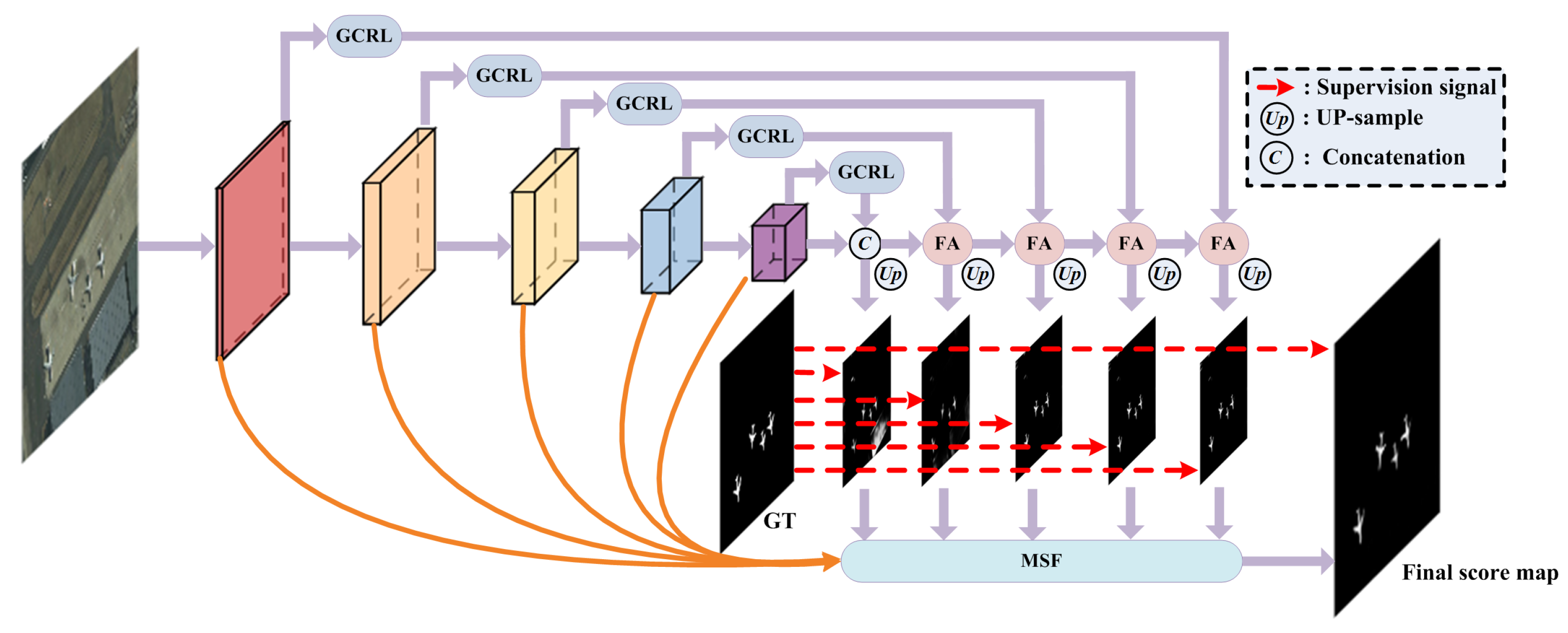
  • We design a global context relation learning module to capture the scattered distribution of salient objects in remote sensing images. In order to exploit the high-level semantic information as well as the low-level appearance details, we propose a global context relation-guided feature aggregation module to refine the initial saliency score map in a progressive manner.
  • Instead of using traditional binary cross entropy as training loss, which treats all pixels equally, we embed a weighted binary cross entropy to capture local surrounding information of different pixels, which can ensure that the pixels located in hard areas such as edges and holes can be assigned with larger weight.
There is a large number of methods proposed for salient object detection of natural images, and many natural image salient object detection methods have been deployed for remote sensing images. Below, we give a brief review of previous salient object detection methods that were designed for natural images as well as for remote sensing images.
Salient object detection for natural images. In earlier years, most of salient object detection methods were often prior-driven and unsupervised, which adopt hand-crafted low-level visual features such as color, texture, spatial location [28,29,30] or heuristic priors such as center prior [31] and boundary prior [32,33]. Although these hand-crafted feature-based methods make remarkable progress, the low-level features and priors are not enough to understand the image scene in a high-level manner, i.e., lacking semantic information of image contents, which results in unsatisfactory saliency maps. Motivated by the rapid popularity of deep neural networks used in computer vision, the performance for different image salient object detection methods have also been promoted with a big step by using deep learning techniques. The main idea of deep neural network-based salient object detection aims to integrate different levels of feature maps for locating salient objects as well as preserving the appearance details [8,9,34,35,36,37,38]. Apart from RGB image source, many other information sources are also used to assist salient object detection for natural images, e.g., depth image [39,40,41,42], image labels/tags and image captions [43,44,45]. The depth image can provide an extra 3D structure of the scene, which can help separate those salient objects with highly similar colors and textures to the background. The image tags and captions can be plugged into a multi-task framework, in which the salient objects can be learned to boost the classification task.
Salient object detection for remote sensing images. Driven by the strong capability of feature extraction for image data [46], many convolutional neural network (CNN)-based salient object detection methods for optical remote sensing images have been put forward. For example, Zhao et al. [47] proposed to use a sparse learning model for extracting both global context information and background noise to locate salient objects in remote sensing images. With regard to the special case of building extraction, Li et al. [48] combined the boundary connectivity, region contrast, as well as background constraints to calculate saliency values of buildings. The contrast of a multi-level color histogram is also utilized to generate the saliency in a hierarchical manner for different regions of interest [49]. Since knowledge is seldom used in image saliency detection, in [50], knowledge-oriented saliency and vision-oriented saliency are combined to help locate the airport from a remote sensing image. In [51], Li et al., proposed an end-to-end deep neural network for remote-sensing-image salient object detection. In LV-Net, a two-stream pyramid module (named the L-shaped module) is designed to extract a set of hierarchical deep features which can perceive the scale diversity and local details of salient objects. Then, an encoder–decoder module with nested connections (named the V-shaped module) is developed to gradually integrate low-level details and semantic features by using nested connections, which helps suppress the background clutters as well as highlight the salient objects. In addition, they constructed the first public remote sensing image dataset (ORSSD) for salient object detection, which contains 800 remote sensing images with their corresponding manually annotated ground truths. Li et al. [52] proposed a fusion network in a parallel down–up manner for detecting salient objects from remote sensing images. In order to highlight the diversely scaled salient objects, it takes successive down-sampling operations for capturing varied scale information. In addition, feature aggregation is also a widely used strategy for saliency detection in remote sensing images. For example, in [19], Zhang et al., generated the edge map to supervise the network training for preserving the details of the final saliency map. Multi-level features are extracted by a CNN backbone and fused with other geometric information such as edge for enhancing salient object boundary [23]. In order to adapt to lightweighted application scenarios, lightweight salient object detection in optical remote sensing images has also become a hot research field [24,26]. Since the global contextual information is very important for understanding remote sensing images, the local-to-contextual paradigm is widely used in recent works for exploring the relation between global and local feature embeddings [25,53,54,55], in which the transformer structure is a typical one [17,18].
Although remarkable success has also been achieved by using deep neural networks for detecting salient objects in remote sensing images, there are still several major issues that need to be noted. Firstly, different salient objects with diverse scales are hard to be accurately detected simultaneously. Secondly, the global context relation of scattered objects has not been fully exploited to enhance the detection results.

2. Materials

Datasets

In this work, we conduct experiments on three public datasets: ORSSD [51], EORSSD [19], and ORSI-4199 [21]. The detailed information of these datasets are as follows:
ORSSD contains 800 images and the corresponding pixel-level annotated binary map, in which 600 images are used for training and the remaining 200 are used for testing.
EORSSD is an extension of ORSSD. Compared to ORSSD, there are 1200 newly collected images. Therefore, there are a total of 2000 images in EORSSD, in which 1400 images are used for model training and the remaining 600 are used for testing.
ORSI-4199 is the biggest dataset for remote-sensing-image salient object detection, it contains 4199 images with pixel-level ground truths, in which 2000 images are used for training and the remaining 2199 are used for testing.

3. Methods

In this work, we introduce a novel end-to-end deep neural network for accurately detecting salient objects from remote sensing scenes by exploring the global context relation of different regions, which plays an important role in remote sensing images.

3.1. Overview

As illustrated in Figure 2, we take the ResNet architecture [56] as the backbone to extract multi-level features and the parameters are initialized by the pre-trained ResNeXt network, which is trained on the ImageNet dataset [57]. Therefore, given an input image, we can obtain five levels of hierarchical features, including conv1, conv2_x, conv3_x, conv4_x, and conv5_x. Since the conv5_x contains abundant high-level features which are beneficial to locate salient objects, we utilize conv5_x to generate an initial saliency score map. However, due to a succession of convolution and pooling operations, the appearance details of image contents are significantly lost in conv5_x. In order to tackle this issue, we design a feature aggregation module (FA) and insert it into the proposed framework to refine the initial output in a progressive manner by capturing both high-level semantic information and low-level details. Since the objects in remote sensing images are often scattered due to the large observation range, the global context relation should also be taken into consideration. Therefore, we develop a global context relation learning module (GCRL) and utilize its learned features to guide the feature aggregation progress. For each feature aggregation stage, we generate an intermediate score map that captures a certain scale of information of the corresponding feature extraction layer. Finally, we introduce a multi-scale fusion module (MSF) to fuse the multiple intermediate score maps of different feature aggregation stages and obtain the final saliency score map.

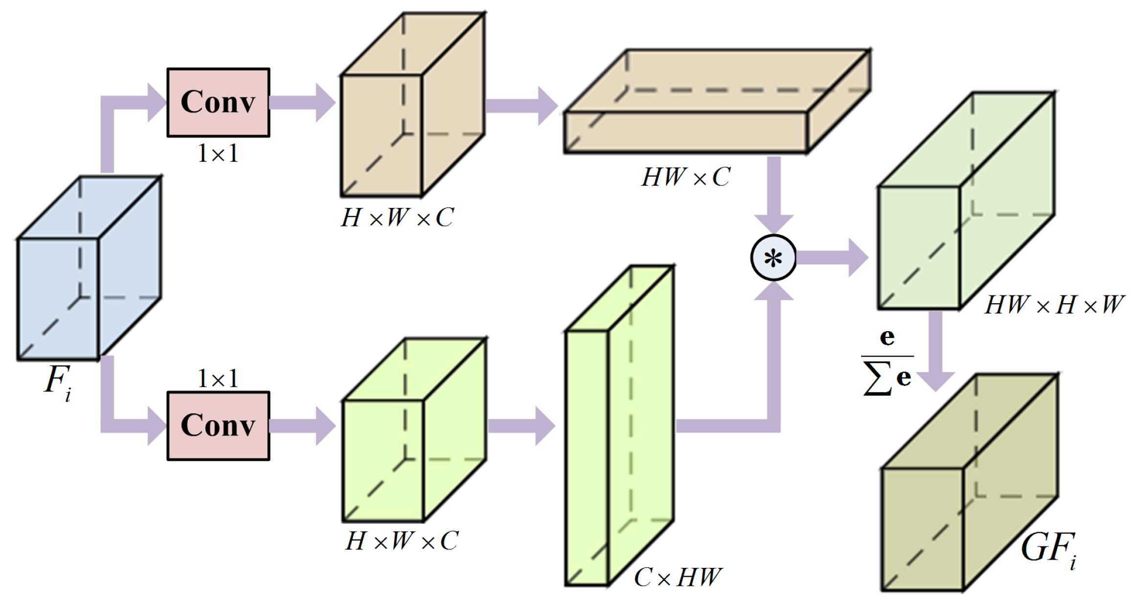
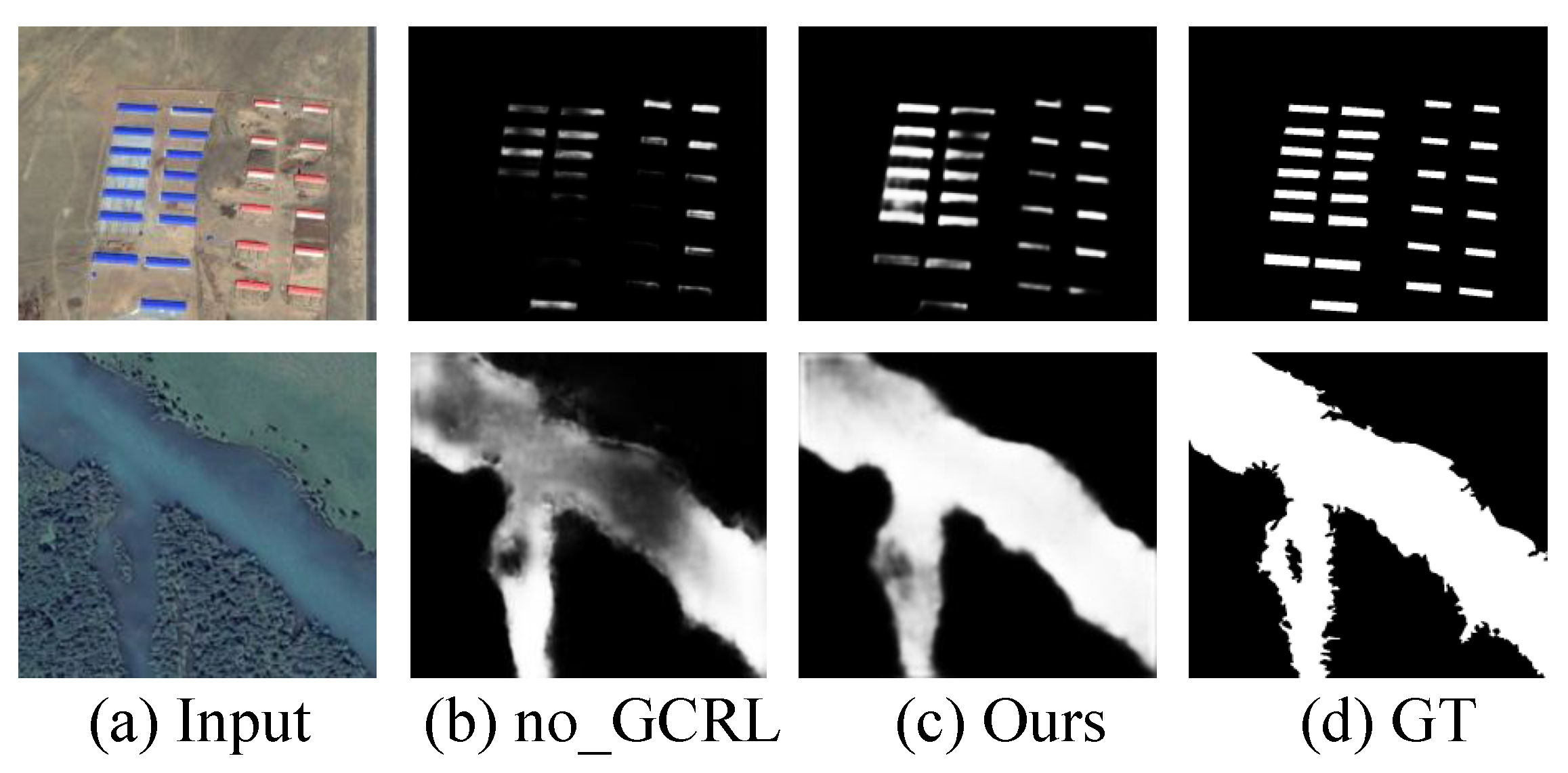
3.2. Global Context Relation Learning Module (GCRL)

For a given remote sensing image, there are usually some challenging cases such as cluttered background and scattered object distribution. Therefore, the global context relationship among multiple salient objects as well as the different parts of a certain salient object should be exploited to boost the saliency map. In this section, we introduce a GCRL module to learn the global context information and utilize it to guide the feature aggregation process in each stage. The structure of each GCRL module is shown in Figure 3.
For two spatial position indices p and q in the i-th-layer feature map F i R H × W × C , we define their global context relationship G C R ( f p , f q ) as follows:
G C R ( f p , f q ) = Φ ( Ψ ( f p , f q ) ) ,
where f p and f q are two feature vectors with size 1 × 1 × C . In linear algebra, a simple way to describe the relationship between two feature vectors is through the dot production. Therefore, for simplicity and computational efficiency, we use dot production operation to calculate the relationship between f p and f q , and then, we define Ψ ( f p , f q ) as follows:
Ψ ( f p , f q ) = w 1 ( f p ) T w 2 ( f q ) ,
where w 1 ( f p ) and w 2 ( f q ) can be obtained by using two different convolution layers. In our GCRL module, we use two 1 × 1 convolution layers to obtain w 1 ( F ) and w 2 ( F ) from F i . Then, we reshape and transpose w 1 ( F ) and w 2 ( F ) to H W × C and C × H W , respectively. By using a simple matrix multiplication, we obtain a H W × H W matrix, which we further reshape to form a global context relation feature GF i of size H × W × H W . Finally, we apply a softmax layer to eliminate negative spatial relations, which is defined as
Φ ( GF i , p q ) = exp ( GF i , p q ) p , q = 1 W × H exp ( GF i , p q ) .
By using the abovementioned GCRL module, global relationships between any two spatial positions in deep feature maps can be fully exploited to further enhance feature representations, especially for haphazardly distributed salient objects, which is very unusual in remote sensing images. In our experiments, we will intuitively demonstrate the efficacy of the proposed GCRL module.
It should be noted that our proposed GCRL module is quite different to previous non-local (NL) neural networks [58] and global context learning networks [59]. Previous NL blocks were actually formed via the generalization of the self-attention mechanism and they would compute the response at a position as a weighted sum of the features at all positions. For the work proposed in [59], it captures global context information in the segmentation process, which weighs the response at a feature location by features at all locations in the input feature map, and the weights are determined based on the feature similarity between two corresponding locations. On the contrary, our proposed GCRL dose not learn the weighted features, but learns the global context relationships for different parts of a remote sensing scene. Therefore, the output of each GCRL is not just weighted features, but reflects spatial context relationships of a certain remote sensing scene. In addition, the output of each GCRL module is used to guide the feature aggregation process in each step.

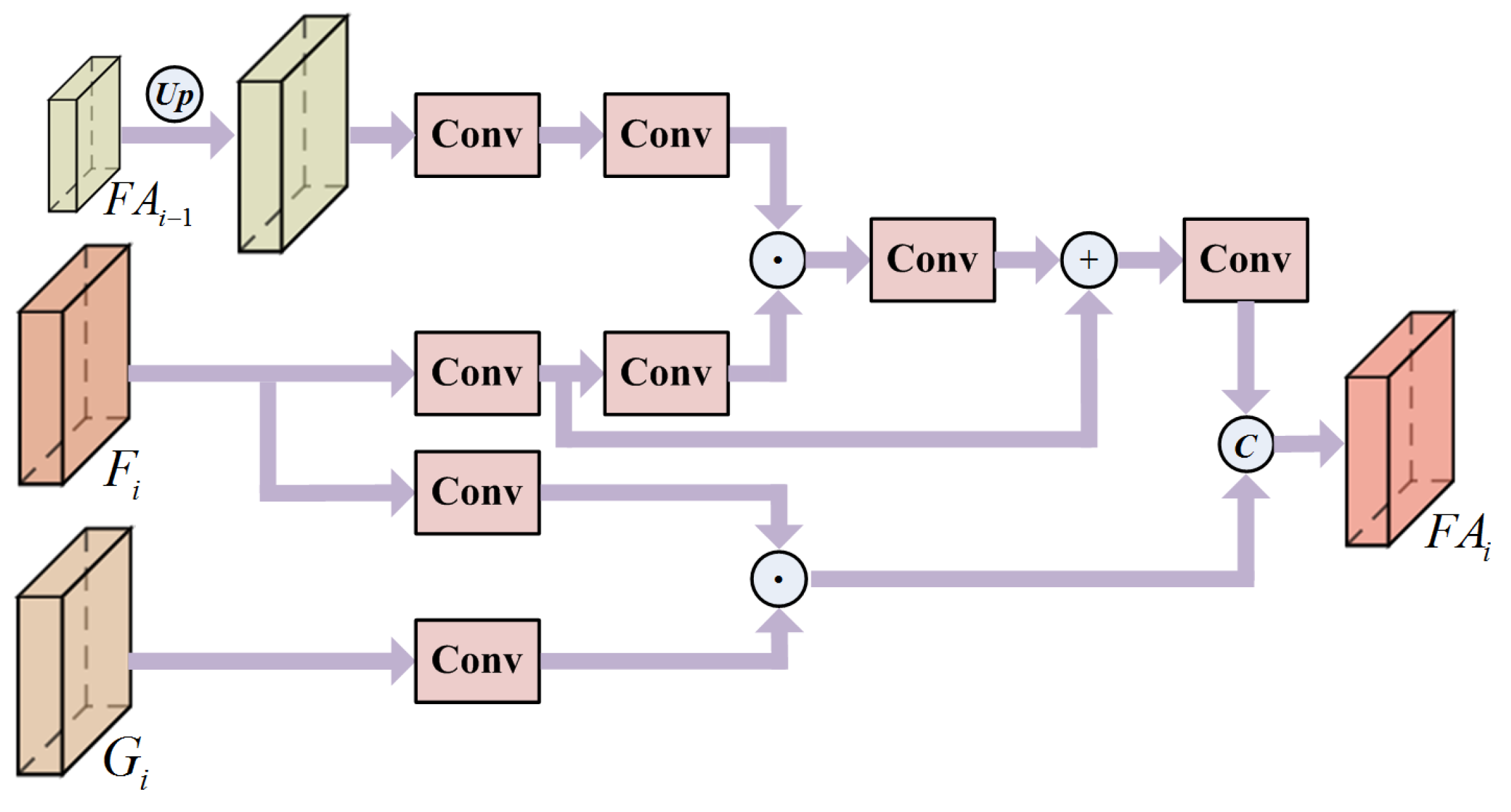
3.3. Feature Aggregation Module (FA)

It is well known that both the high-level semantic information and low-level details are important for pixel-wise salient object detection. Therefore, the way in which to integrate the features extracted from different network layers is critical. A simple and commonly used operation in previous methods is concatenation. However, through this method, the complementary information between different layers of features cannot be fully captured, and the noisy and redundant features cannot be effectively eliminated. In this paper, a feature aggregation module is proposed to fully integrate low-level detail features, high-level semantic features, as well as global context relation information to suppress the background noises and recover more structural and semantic information.
Supposing that the feature maps of the i-th layer, the global context relation of the i-th layer, and the output of the ( i 1 ) -th FA module are denoted as F i , G i and FA i 1 , respectively, then the output of the i-th FA module can be obtained via the flowchart from Figure 4. The proposed FA module aims to preserve the consistency and suppress the inconsistency between F i and FA i 1 . Instead of directly using common addition or concatenation for feature integration in most existing studies, we firstly extract the consistent parts between F i and FA i 1 by element-wise multiplication. In such a manner, the common parts of cross-level features can be enhanced while the inconsistent parts can be weakened. Then, we combine F i and the enhanced features F i , m by element-wise addition for retaining a part of the information from layer-wise features. In addition, in order to enhance the global context relation information of the integrated features, we embed G i into each FA module to guide the feature aggregation. Since the feature channel of G i is different to F i , we first use a convolution operation to adapt G i to F i . After obtaining the global context relation-enhanced feature by multiplying the adapted G i with F i , we combine it with F i , m by concatenation to obtain the output of the i-th FA module FA i . Mathematically, the features obtained by multiplication F i , m and F i can be generated as follows:
F i , m = W i , 2 ( W i , 1 ( FA i 1 ) ) W i , 4 ( W i , 3 ( F i ) ) , FA i = C a t ( W i , 6 ( W i , 5 ( F i , m ) + W i , 3 ( F i ) ) , W i , 7 ( F i ) W i , 8 ( G i ) ) ,
where W i , k ( k = 1 , 2 , , 8 ) is the k-th combination of convolution, batch normalization and ReLU operations of the i-th FA module, Cat represents the concatenation operation, and ∗ represents element-wise multiplication.
It should be noted that each “Conv” block in both the GCRL and FA modules is actually a combination with batch normalization and activation, which is the so called “convolution block”. There are no residual connections in the block. We simply use the ResNet architecture as the backbone for feature extraction, which consists of a series of residual connections for avoiding gradient vanishing. However, in our proposed modules, we only use the extracted features for salient object detection, so we do not use any residual connection in the convolution block. Since there are only a small number of convolution blocks compared to the backbone, the gradient vanishing phenomenon does not happen in our network.

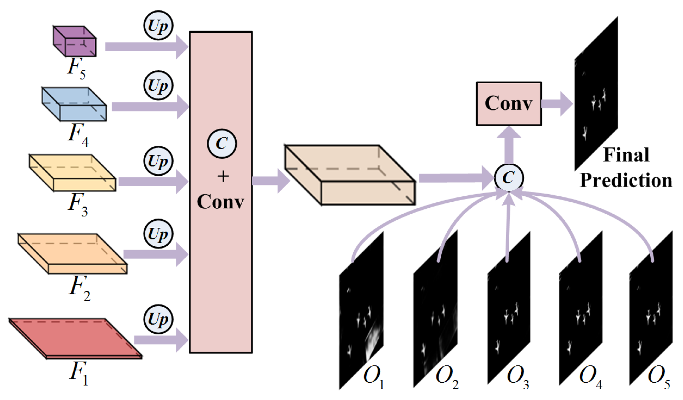
3.4. Multi-Scale Fusion Module (MSF)

Since different levels of features capture different scale information of the original images, the outputs of different FA modules can be used to help detect salient objects with varying sizes. Therefore, we design an MSF module to combine the multiple intermediate outputs to generate the final saliency score map. In addition, we also utilize original hierarchical features extracted from the backbone network to guide the fusion process. Although many previous works use the fusion strategy to fuse multiple outputs, they ignore the deep features extracted by shallow layers. The structure of our designed MSF module is shown in Figure 5. We first concatenate F 1 , F 2 , F 3 , F 4 and F 5 together and reduce the channel dimension of the concatenated features by using a convolution. Then, the five side outputs are combined with the reduced features to obtain the final prediction result S . The whole process can be mathematically described as follows:
F c = C a t ( U p ( F 1 ) , U p ( F 2 ) , U p ( F 3 ) , U p ( F 4 ) , U p ( F 5 ) ) , S = G 2 ( C a t ( G 1 ( F c ) , O 1 , O 2 , O 3 , O 4 , O 5 ) ) ,
where Up represents the up-sampling operation; F c is the concatenated feature of different layers; G 1 and G 2 are two convolution operations; and O 1 , O 2 , O 3 , O 4 and O 5 represent the output of the five feature aggregation modules, respectively.

3.5. Local Surrounding Aware Loss

In previous works, binary cross entropy (BCE) is the most widely used loss function for network training. However, BCE treats each pixel equally and calculates the loss for each pixel independently, and so, the local surrounding information of each pixel is not captured. In fact, pixels located on cluttered or boundary areas should be given more attention since these pixels are often with complex local surrounding structures. Therefore, we propose to design a local surrounding aware loss ( L S A ) as follows:
L S A = i = 1 H j = 1 W ω i j L B C E i j i = 1 H j = 1 W ω i j L B C E i j i = 1 H j = 1 W ω i j i = 1 H j = 1 W ω i j ,
where L B C E i j and ω i j are the traditional BCE loss and the weight for the i j -th pixel, respectively. Given the ground truth saliency map (GT) of a training image, the weight map of all its pixels can be calculated as follows:
W = Φ ( G T ) G T ,
where Φ ( · ) is a mapping function to calculate the surrounding information of pixels. In this work, we use the average pooling operation to implement Φ ( · ) . In such a manner, pixels located in hard areas such as edges and holes will be assigned with larger weight.

3.6. Model Training and Testing

Training: As mentioned in the previous section, we initialize our proposed network by the well-trained ResNeXt network (ResNeXt-50) on ImageNet [57]. The size of the pre-trained ResNeXt-50 model is 191 MB. After we add the designed modules, the size of our final trained model is 205 MB. Therefore, the increment of the model size is only about 7.2%. For each dataset, we divide it into two parts, one for training and the rest for testing.
Testing: During testing, for an input image, we feed it into our trained network and obtain the final saliency score map.
Implementation Details: Our proposed network is implemented by using the PyTorch library on a PC with an Intel Xeon ES-2603 v4 CPU, 32 GB RAM, and an NVIDIA GeForce GTX 1080Ti GPU. During training, the batch size (the number of training samples in each iteration) is set to 8. The whole network is optimized by using the Stochastic gradient descent (SGD) algorithm with a momentum of 0.9 and a weight decay of 0.0005. We adjust the learning rate by the “poly” policy with a power of 0.9. We stop the whole learning process after 10k iterations. The whole training process costs about 1.5 h. The code will be released with this paper for public academic usage.
Loss Function: In this work, we use the local surrounding aware loss for each side output and the final output during the training process, which can be calculated as follows:
L = L S A d + k = 1 5 L S A k ,
where L S A k represents the loss for the k-th side output, L S A d is dominant loss for the final output layer.

4. Results

4.1. Evaluation Metrics

In order to validate the efficacy of the proposed network, we use six widely used metrics for a quantitative performance evaluation: the S-measure ( S α , α = 0.5 ) [60], F-measure ( F β , β 2 = 0.3 ) [61], E-measure ( E ξ ) [62], mean absolute error scores (MAE, M ), a precision–recall (PR) curve and an F-measure curve. As an overall performance measurement, the F-measure is defined as
F β = 1 + β 2 · p r e c i s i o n · r e c a l l β 2 · p r e c i s i o n + r e c a l l .
As neither the precision nor recall measure evaluate the true negative saliency assignments, we use the mean absolute error (MAE) as a complementary. The MAE score calculates the average difference between the detected saliency score map S and the ground truth G , it is computed as
M A E = 1 W × H x = 1 W y = 1 H | S ( x , y ) G ( x , y ) | ,
where H and W are the height and width of the input image, respectively.

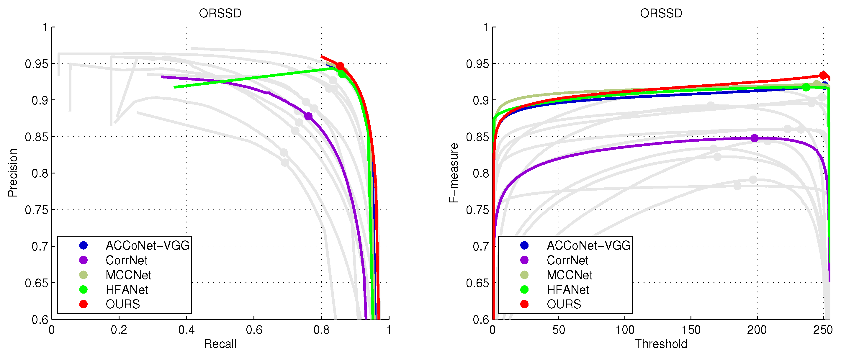
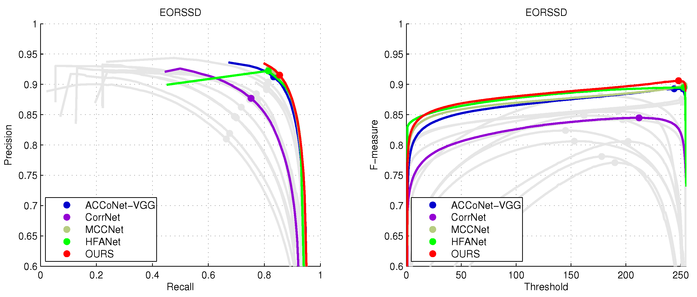
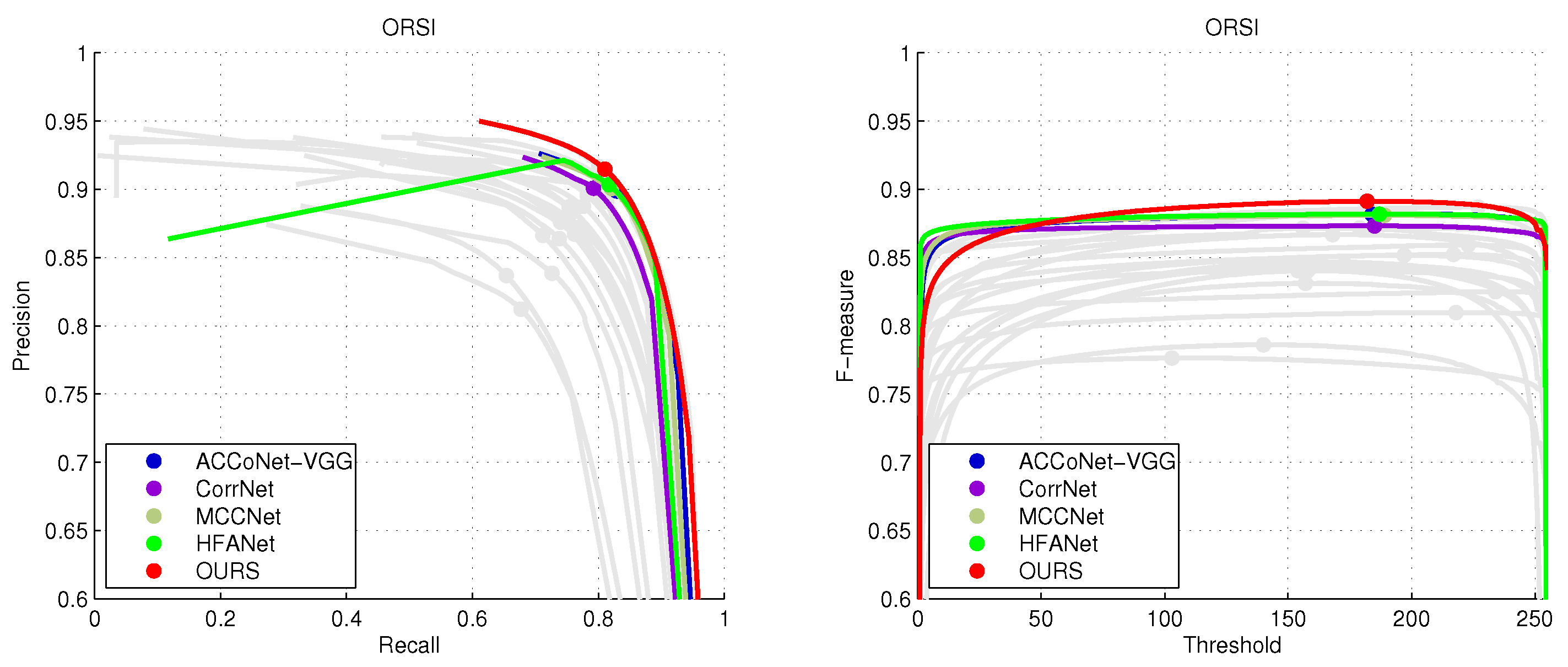
4.2. Comparison with State-of-the-Art Methods

In order to validate the efficacy of our proposed network, we compare its performance with other 24 salient object detection methods, including 17 traditional natural image salient object detection models and 7 optical remote-sensing-image salient object detection models. The compared methods are R3Net [63], PiCANet [64], PoolNet [65], EGNet [66], BASNet [67], CPD [68], RAS [69], CSNet [70], SAMNet [71], HVPNet [72], ENFNet [73], SUCA [74], PA-KRN [75], VST [76], DPORTNet-VGG [77], DNTD-Res [78], ICON-PVT [79], MJRBMVGG [21], EMFINetVGG [25], ERPNetVGG [23], ACCoNet-VGG [27], CorrNet [24], MCCNet [20] and HFANet [80]. Among these methods, the last seven ones are specifically designed for salient object detection in remote sensing images.
Quantitative Comparison. In Table 1 and Table 2, we report the compared results of different metrics obtained by different models implemented on the three datasets. With regard to the ORSSD dataset, it can be observed that our proposed network consistently performs favourably against other methods. With regard to the ORSSD and ORSI-4199 datasets, our method also performs better than other competitors in nearly all cases. In Figure 6, Figure 7 and Figure 8, we plot the PR curves and F-measure curves of different methods on different datasets (since there are 24 salient object detection methods used for comparison in this paper, which inevitably produce many curves in different figures; therefore, in order to make the comparison in figures clearer, we intentionally make some of the curves gray and only label those curves corresponding to some representative or competitive methods with names). From the results, we observe that our method also consistently outperforms other counterparts on the three datasets.
Qualitative Comparison. In order to give a more intuitive illustration of the comparison of the results, we show some visual results of our proposed network and others in Figure 9. As can be seen, our method generates more accurate saliency score maps when the input images contain background clutter. In addition, the boundaries of the salient objects can be well preserved in our results. It should be noted that when the salient objects are slender, our proposed network can also obtain good results. In addition, as to many other challenging cases such as varying object shapes, sizes and orientations, our proposed network can also handle well. Therefore, the high-level semantics information, low-level details as well as different scale information can be well captured by our proposed network.

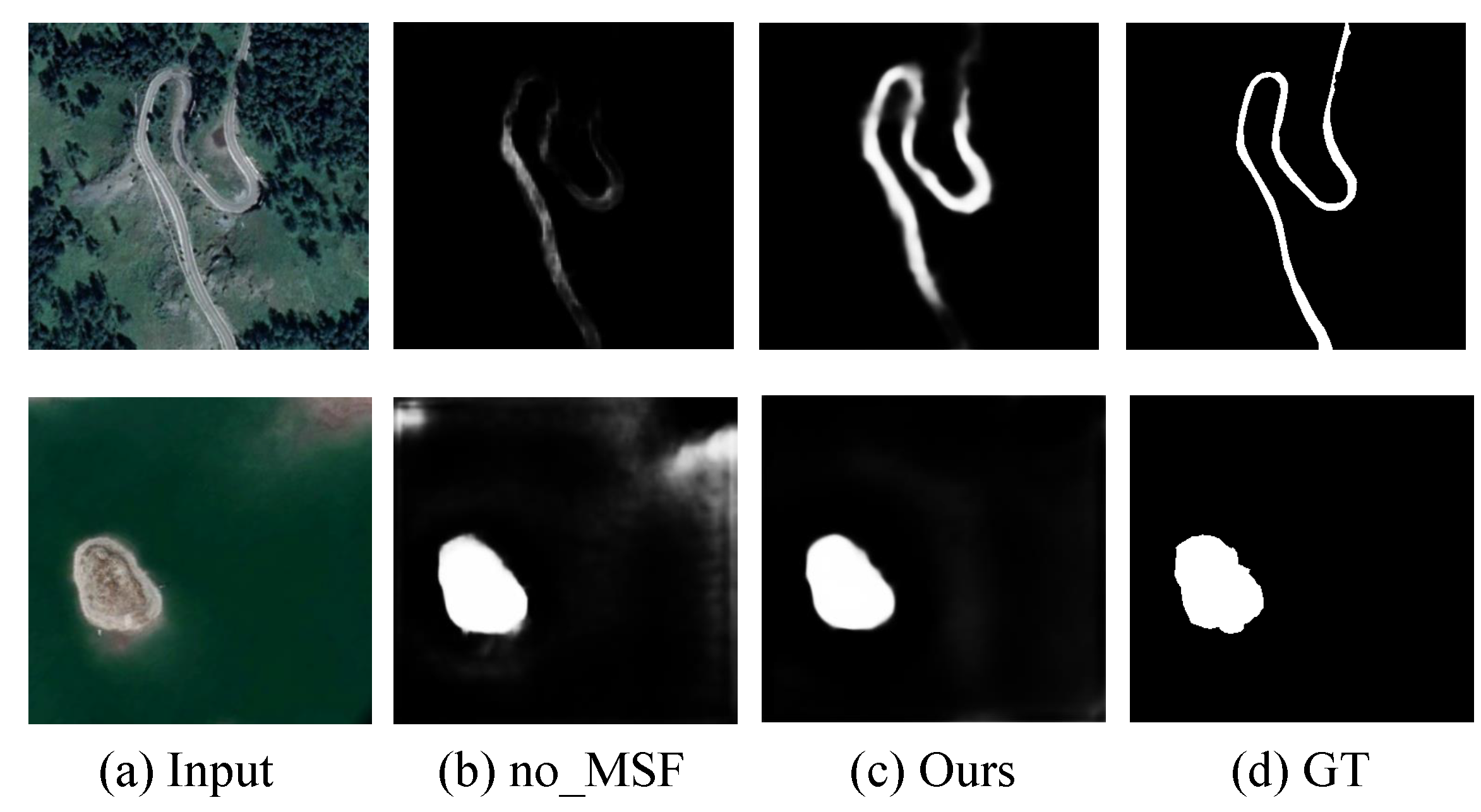
4.3. Ablation Analysis

Effectiveness of GCRL module. In this work, we design the GCRL module to learn the global context relation information to guide the feature aggregation process. In order to demonstrate the efficacy of this module, we remove it from our network, i.e., there is no G i in Figure 4 (denoted as no_GCRL), and the results are shown in Figure 10. As can be seen from the results, when the network is without the GCRL module, some scattered objects cannot be detected well simultaneously (see the blue factory buildings in the first image). With the GCRL module, our network can detect scattered salient objects.
Effectiveness of the MSF module. In order to validate the efficacy of the proposed MSF module, we give an intuitive presentation of the results with/without MSF in Figure 11. As can be seen, if we directly use the output of the final FA module as the saliency score map (no_MSF), the salient objects can be roughly located, but the details are lost. On the contrary, if we use the MSF module to fuse the side outputs of different FA modules, the high-level semantic information and low-level details can be well preserved.
In Table 3, we also display the quantitative ablation analysis results of GCRL and MSF modules. “OURS_noGCRL” means the proposed network without the GCRL modules, and “OURS_noMSF” means the proposed network without the MSF module. As can be seen from the results, both the GCRL and MSF modules show obvious improvement for the final results, which validates the efficacy of the designed modules in the proposed network.

4.4. Running Efficiency Comparison

In order to show the intuitive efficiency of the proposed network, we compare its inferring time with other methods on different datasets in Table 4. For eliminating bias caused by different sizes of different images in each dataset, we report the average inferring time (seconds) for a single image in different datasets. As can be seen, although the proposed network does not perform the fastest, it still outperforms most of other competitors.

5. Conclusions

In this work, we propose an end-to-end deep neural network for salient object detection from remote sensing images. In order to capture the global context relation of scattered objects, we propose a global context relation learning model. Since both the high-level semantic information and low-level details are important for final results, we design a feature aggregation module and embed it into the network for feature boosting. The learned global context relation is also used to guide the feature aggregation in each stage. The side outputs of different FA modules are fused to generate the final result. In addition, instead of using traditional binary cross entropy as the training loss, which treats all pixels equally, we design a weighted binary cross entropy to capture local surrounding information of different pixels. In order to promote further study of this field, we collect a new dataset which consists of various challenging images and their pixel-wise annotations. Extensive experiments on previous datasets and our newly collected one are conducted to validate the efficiency of the proposed network.

Author Contributions

Methodology, J.L., C.L. and X.Z.; Validation, C.L.; Formal analysis, X.L. and C.T.; Investigation, X.Z. and X.L.; Writing—original draft, J.L.; Supervision, C.T. All authors have read and agreed to the published version of the manuscript.

Funding

This work was supported in part by the National Natural Science Foundation of China (No. 62101512 and 62271453), and in part by the Fundamental Research Program of Shanxi Province (20210302124031) and Shanxi Scholarship Council of China (2023-131).

Data Availability Statement

The original contributions presented in the study are included in the article, further inquiries can be directed to the corresponding author.

Conflicts of Interest

The authors declare no conflicts of interest.

References

  1. Zhang, Z.; Davaasuren, D.; Wu, C.; Goldstein, J.A.; Gernand, A.D.; Wang, J.Z. Multi-region Saliency-aware Learning for Cross-domain Placenta Image Segmentation. Pattern Recognit. Lett. 2020, 140, 165–171. [Google Scholar] [CrossRef] [PubMed]
  2. Wang, W.; Shen, J.; Yang, R.; Porikli, F. Saliency-aware video object segmentation. IEEE Trans. Pattern Anal. Mach. Intell. 2017, 40, 20–33. [Google Scholar] [CrossRef] [PubMed]
  3. Battiato, S.; Farinella, G.M.; Puglisi, G.; Ravi, D. Saliency-based selection of gradient vector flow paths for content aware image resizing. IEEE Trans. Image Process. 2014, 23, 2081–2095. [Google Scholar] [CrossRef] [PubMed]
  4. Cho, D.; Park, J.; Oh, T.H.; Tai, Y.W.; So Kweon, I. Weakly-and self-supervised learning for content-aware deep image retargeting. In Proceedings of the IEEE International Conference on Computer Vision, Venice, Italy, 22–29 October 2017; pp. 4558–4567. [Google Scholar]
  5. Zhang, L.; Shen, Y.; Li, H. VSI: A visual saliency-induced index for perceptual image quality assessment. IEEE Trans. Image Process. 2014, 23, 4270–4281. [Google Scholar] [CrossRef] [PubMed]
  6. Oszust, M. No-Reference quality assessment of noisy images with local features and visual saliency models. Inf. Sci. 2019, 482, 334–349. [Google Scholar] [CrossRef]
  7. Liu, L.; Ouyang, W.; Wang, X.; Fieguth, P.; Chen, J.; Liu, X.; Pietikäinen, M. Deep learning for generic object detection: A survey. Int. J. Comput. Vis. 2020, 128, 261–318. [Google Scholar] [CrossRef]
  8. Pang, Y.; Zhao, X.; Zhang, L.; Lu, H. Multi-Scale Interactive Network for Salient Object Detection. In Proceedings of the IEEE/CVF Conference on Computer Vision and Pattern Recognition, Seattle, WA, USA, 13–19 June 2020; pp. 9413–9422. [Google Scholar]
  9. Zhang, L.; Wu, J.; Wang, T.; Borji, A.; Wei, G.; Lu, H. A Multistage Refinement Network for Salient Object Detection. IEEE Trans. Image Process. 2020, 29, 3534–3545. [Google Scholar] [CrossRef]
  10. Zhou, S.; Wang, J.; Zhang, J.; Wang, L.; Huang, D.; Du, S.; Zheng, N. Hierarchical U-Shape Attention Network for Salient Object Detection. IEEE Trans. Image Process. 2020, 29, 8417–8428. [Google Scholar] [CrossRef]
  11. Zhang, J.; Yu, X.; Li, A.; Song, P.; Liu, B.; Dai, Y. Weakly-Supervised Salient Object Detection via Scribble Annotations. In Proceedings of the IEEE/CVF Conference on Computer Vision and Pattern Recognition, Seattle, WA, USA, 13–19 June 2020; pp. 12546–12555. [Google Scholar]
  12. Wei, J.; Wang, S.; Wu, Z.; Su, C.; Huang, Q.; Tian, Q. Label Decoupling Framework for Salient Object Detection. In Proceedings of the IEEE/CVF Conference on Computer Vision and Pattern Recognition, Seattle, WA, USA, 13–19 June 2020; pp. 13025–13034. [Google Scholar]
  13. Fu, K.; Fan, D.P.; Ji, G.P.; Zhao, Q. Jl-dcf: Joint learning and densely-cooperative fusion framework for rgb-d salient object detection. In Proceedings of the IEEE/CVF Conference on Computer Vision and Pattern Recognition, Seattle, WA, USA, 13–19 June 2020; pp. 3052–3062. [Google Scholar]
  14. Piao, Y.; Rong, Z.; Zhang, M.; Ren, W.; Lu, H. A2dele: Adaptive and Attentive Depth Distiller for Efficient RGB-D Salient Object Detection. In Proceedings of the IEEE/CVF Conference on Computer Vision and Pattern Recognition, Seattle, WA, USA, 13–19 June 2020; pp. 9060–9069. [Google Scholar]
  15. He, X.; Tang, C.; Liu, X.; Zhang, W.; Sun, K.; Xu, J. Object detection in hyperspectral image via unified spectral-spatial feature aggregation. IEEE Trans. Geosci. Remote Sens. 2023, 61, 5521213. [Google Scholar] [CrossRef]
  16. Tang, C.; Wang, J.; Zheng, X.; Liu, X.; Xie, W.; Li, X.; Zhu, X. Spatial and spectral structure preserved self-representation for unsupervised hyperspectral band selection. IEEE Trans. Geosci. Remote Sens. 2023, 61, 5531413. [Google Scholar] [CrossRef]
  17. Li, G.; Bai, Z.; Liu, Z.; Zhang, X.; Ling, H. Salient object detection in optical remote sensing images driven by transformer. IEEE Trans. Image Process. 2023, 32, 5257–5269. [Google Scholar] [CrossRef] [PubMed]
  18. Yan, R.; Yan, L.; Geng, G.; Cao, Y.; Zhou, P.; Meng, Y. ASNet: Adaptive Semantic Network Based on Transformer-CNN for Salient Object Detection in Optical Remote Sensing Images. IEEE Trans. Geosci. Remote Sens. 2024, 62, 5608716. [Google Scholar] [CrossRef]
  19. Zhang, Q.; Cong, R.; Li, C.; Cheng, M.M.; Fang, Y.; Cao, X.; Zhao, Y.; Kwong, S. Dense Attention Fluid Network for Salient Object Detection in Optical Remote Sensing Images. IEEE Trans. Image Process. 2020, 30, 1305–1317. [Google Scholar] [CrossRef] [PubMed]
  20. Li, G.; Liu, Z.; Lin, W.; Ling, H. Multi-content complementation network for salient object detection in optical remote sensing images. IEEE Trans. Geosci. Remote Sens. 2022, 60, 5614513. [Google Scholar] [CrossRef]
  21. Tu, Z.; Wang, C.; Li, C.; Fan, M.; Zhao, H.; Luo, B. ORSI salient object detection via multiscale joint region and boundary model. IEEE Trans. Geosci. Remote Sens. 2022, 60, 5607913. [Google Scholar] [CrossRef]
  22. Cong, R.; Zhang, Y.; Fang, L.; Li, J.; Zhao, Y.; Kwong, S. RRNet: Relational reasoning network with parallel multiscale attention for salient object detection in optical remote sensing images. IEEE Trans. Geosci. Remote Sens. 2021, 60, 5613311. [Google Scholar] [CrossRef]
  23. Zhou, X.; Shen, K.; Weng, L.; Cong, R.; Zheng, B.; Zhang, J.; Yan, C. Edge-guided recurrent positioning network for salient object detection in optical remote sensing images. IEEE Trans. Cybern. 2023, 53, 539–552. [Google Scholar] [CrossRef] [PubMed]
  24. GongyangLi, Z.; Bai, Z.; Lin, W.; Ling, H. Lightweight salient object detection in optical remote sensing images via feature correlation. IEEE Trans. Geosci. Remote Sens. 2022, 60, 5617712. [Google Scholar]
  25. Wang, Z.; Guo, J.; Zhang, C.; Wang, B. Multiscale feature enhancement network for salient object detection in optical remote sensing images. IEEE Trans. Geosci. Remote Sens. 2022, 60, 5634819. [Google Scholar] [CrossRef]
  26. Li, G.; Liu, Z.; Zhang, X.; Lin, W. Lightweight salient object detection in optical remote-sensing images via semantic matching and edge alignment. IEEE Trans. Geosci. Remote Sens. 2023, 60, 5617712. [Google Scholar] [CrossRef]
  27. Li, G.; Liu, Z.; Zeng, D.; Lin, W.; Ling, H. Adjacent context coordination network for salient object detection in optical remote sensing images. IEEE Trans. Cybern. 2023, 53, 526–538. [Google Scholar] [CrossRef]
  28. Cheng, M.M.; Mitra, N.J.; Huang, X.; Torr, P.H.; Hu, S.M. Global contrast based salient region detection. IEEE Trans. Pattern Anal. Mach. Intell. 2014, 37, 569–582. [Google Scholar] [CrossRef]
  29. Wang, J.; Tang, C.; Zheng, X.; Liu, X.; Zhang, W.; Zhu, E.; Zhu, X. Fast approximated multiple kernel k-means. IEEE Trans. Knowl. Data Eng. 2023, 1–10. [Google Scholar] [CrossRef]
  30. Wang, J.; Tang, C.; Wan, Z.; Zhang, W.; Sun, K.; Zomaya, A.Y. Efficient and effective one-step multiview clustering. IEEE Trans. Neural Netw. Learn. Syst. 2023, 1–12. [Google Scholar] [CrossRef]
  31. Chen, S.; Zheng, L.; Hu, X.; Zhou, P. Discriminative saliency propagation with sink points. Pattern Recognit. 2016, 60, 2–12. [Google Scholar] [CrossRef]
  32. Zhu, W.; Liang, S.; Wei, Y.; Sun, J. Saliency optimization from robust background detection. In Proceedings of the IEEE Conference on Computer Vision and Pattern Recognition, Columbus, OH, USA, 23–28 June 2014; pp. 2814–2821. [Google Scholar]
  33. Yang, C.; Zhang, L.; Lu, H.; Ruan, X.; Yang, M.H. Saliency detection via graph-based manifold ranking. In Proceedings of the IEEE Conference on Computer Vision and Pattern Recognition, Portland, OR, USA, 23–28 June 2013; pp. 3166–3173. [Google Scholar]
  34. Zhang, P.; Wang, D.; Lu, H.; Wang, H.; Xiang, R. Amulet: Aggregating Multi-level Convolutional Features for Salient Object Detection. In Proceedings of the IEEE International Conference on Computer Vision, Venice, Italy, 22–29 October 2017; pp. 202–211. [Google Scholar]
  35. Hu, X.; Zhu, L.; Qin, J.; Fu, C.W.; Heng, P.A. Recurrently Aggregating Deep Features for Salient Object Detection. In Proceedings of the AAAI Conference on Artificial Intelligence, New Orleans, LA, USA, 2–7 February 2018; pp. 6943–6950. [Google Scholar]
  36. Chen, S.; Tan, X.; Wang, B.; Hu, X. Reverse Attention for Salient Object Detection. In Proceedings of the ECCV, Munich, Germany, 8–14 September 2018. [Google Scholar]
  37. Zhang, X.; Wang, T.; Qi, J.; Lu, H.; Wang, G. Progressive Attention Guided Recurrent Network for Salient Object Detection. In Proceedings of the CVPR, Salt Lake City, UT, USA, 18–23 June 2018. [Google Scholar]
  38. Wang, T.; Zhang, L.; Wang, S.; Lu, H.; Yang, G.; Ruan, X.; Borji, A. Detect Globally, Refine Locally: A Novel Approach to Saliency Detection. In Proceedings of the CVPR, Salt Lake City, UT, USA, 18–23 June 2018. [Google Scholar]
  39. Chen, H.; Li, Y. Progressively complementarity-aware fusion network for RGB-D salient object detection. In Proceedings of the IEEE Conference on Computer Vision and Pattern Recognition, Salt Lake City, UT, USA, 18–23 June 2018; pp. 3051–3060. [Google Scholar]
  40. Liu, N.; Zhang, N.; Han, J. Learning Selective Self-Mutual Attention for RGB-D Saliency Detection. In Proceedings of the IEEE/CVF Conference on Computer Vision and Pattern Recognition, Seattle, WA, USA, 13–19 June 2020; pp. 13756–13765. [Google Scholar]
  41. Fan, D.P.; Lin, Z.; Zhang, Z.; Zhu, M.; Cheng, M.M. Rethinking RGB-D Salient Object Detection: Models, Data Sets, and Large-Scale Benchmarks. IEEE Trans. Neural Netw. Learn. Syst. 2020, 32, 2075–2089. [Google Scholar] [CrossRef]
  42. Li, C.; Cong, R.; Kwong, S.; Hou, J.; Fu, H.; Zhu, G.; Zhang, D.; Huang, Q. ASIF-Net: Attention steered interweave fusion network for RGB-D salient object detection. IEEE Trans. Cybern. 2020, 32, 2075–2089. [Google Scholar] [CrossRef]
  43. Wang, L.; Lu, H.; Wang, Y.; Feng, M.; Wang, D.; Yin, B.; Ruan, X. Learning to detect salient objects with image-level supervision. In Proceedings of the IEEE Conference on Computer Vision and Pattern Recognition, Honolulu, HI, USA, 21–26 July 2017; pp. 136–145. [Google Scholar]
  44. Zhang, L.; Zhang, J.; Lin, Z.; Lu, H.; He, Y. Capsal: Leveraging captioning to boost semantics for salient object detection. In Proceedings of the IEEE Conference on Computer Vision and Pattern Recognition, Long Beach, CA, USA, 15–20 June 2019; pp. 6024–6033. [Google Scholar]
  45. Zeng, Y.; Zhuge, Y.; Lu, H.; Zhang, L.; Qian, M.; Yu, Y. Multi-source weak supervision for saliency detection. In Proceedings of the IEEE Conference on Computer Vision and Pattern Recognition, Long Beach, CA, USA, 15–20 June 2019; pp. 6074–6083. [Google Scholar]
  46. Tang, C.; Liu, X.; Zheng, X.; Li, W.; Xiong, J.; Wang, L.; Zomaya, A.Y.; Longo, A. DeFusionNET: Defocus blur detection via recurrently fusing and refining discriminative multi-scale deep features. IEEE Trans. Pattern Anal. Mach. Intell. 2020, 44, 955–968. [Google Scholar] [CrossRef]
  47. Zhao, D.; Wang, J.; Shi, J.; Jiang, Z. Sparsity-guided saliency detection for remote sensing images. J. Appl. Remote Sens. 2015, 9, 095055. [Google Scholar] [CrossRef]
  48. Li, E.; Xu, S.; Meng, W.; Zhang, X. Building extraction from remotely sensed images by integrating saliency cue. IEEE J. Sel. Top. Appl. Earth Obs. Remote Sens. 2016, 10, 906–919. [Google Scholar] [CrossRef]
  49. Li, T.; Zhang, J.; Lu, X.; Zhang, Y. SDBD: A hierarchical region-of-interest detection approach in large-scale remote sensing image. IEEE Geosci. Remote Sens. Lett. 2017, 14, 699–703. [Google Scholar] [CrossRef]
  50. Zhang, Q.; Zhang, L.; Shi, W.; Liu, Y. Airport extraction via complementary saliency analysis and saliency-oriented active contour model. IEEE Geosci. Remote Sens. Lett. 2018, 15, 1085–1089. [Google Scholar] [CrossRef]
  51. Li, C.; Cong, R.; Hou, J.; Zhang, S.; Qian, Y.; Kwong, S. Nested network with two-stream pyramid for salient object detection in optical remote sensing images. IEEE Trans. Geosci. Remote Sens. 2019, 57, 9156–9166. [Google Scholar] [CrossRef]
  52. Li, C.; Cong, R.; Guo, C.; Li, H.; Zhang, C.; Zheng, F.; Zhao, Y. A parallel down-up fusion network for salient object detection in optical remote sensing images. Neurocomputing 2020, 415, 411–420. [Google Scholar] [CrossRef]
  53. Huang, K.; Li, N.; Huang, J.; Tian, C. Exploiting Memory-based Cross-Image Contexts for Salient Object Detection in Optical Remote Sensing Images. IEEE Trans. Geosci. Remote Sens. 2024, 62, 5614615. [Google Scholar] [CrossRef]
  54. Zhao, R.; Zheng, P.; Zhang, C.; Wang, L. Progressive Complementation Network with Semantics and Details for Salient Object Detection in Optical Remote Sensing Images. IEEE J. Sel. Top. Appl. Earth Obs. Remote Sens. 2024, 17, 8626–8641. [Google Scholar] [CrossRef]
  55. Quan, Y.; Xu, H.; Wang, R.; Guan, Q.; Zheng, J. ORSI Salient Object Detection via Progressive Semantic Flow and Uncertainty-aware Refinement. IEEE Trans. Geosci. Remote Sens. 2024, 62, 5608013. [Google Scholar] [CrossRef]
  56. He, K.; Zhang, X.; Ren, S.; Sun, J. Deep residual learning for image recognition. In Proceedings of the IEEE Conference on Computer Vision and Pattern Recognition, Las Vegas, NV, USA, 27–30 June 2016; pp. 770–778. [Google Scholar]
  57. Xie, S.; Girshick, R.; Dollár, P.; Tu, Z.; He, K. Aggregated residual transformations for deep neural networks. In Proceedings of the IEEE Conference on Computer Vision and Pattern Recognition, Honolulu, HI, USA, 21–26 July 2017; pp. 1492–1500. [Google Scholar]
  58. Wang, X.; Girshick, R.; Gupta, A.; He, K. Non-local neural networks. In Proceedings of the IEEE Conference on Computer Vision and Pattern Recognition, Salt Lake City, UT, USA, 18–23 June 2018; pp. 7794–7803. [Google Scholar]
  59. Lin, C.Y.; Chiu, Y.C.; Ng, H.F.; Shih, T.K.; Lin, K.H. Global-and-local context network for semantic segmentation of street view images. Sensors 2020, 20, 2907. [Google Scholar] [CrossRef]
  60. Cheng, M.M.; Fan, D.P. Structure-measure: A new way to evaluate foreground maps. Int. J. Comput. Vis. 2021, 129, 2622–2638. [Google Scholar] [CrossRef]
  61. Achanta, R.; Hemami, S.; Estrada, F.; Susstrunk, S. Frequency-tuned salient region detection. In Proceedings of the 2009 IEEE Conference on Computer Vision and Pattern Recognition, Miami, FL, USA, 20–25 June 2009; pp. 1597–1604. [Google Scholar]
  62. Fan, D.P.; Gong, C.; Cao, Y.; Ren, B.; Cheng, M.M.; Borji, A. Enhanced-alignment measure for binary foreground map evaluation. In Proceedings of the 27th International Joint Conference on Artificial Intelligence, Stockholm, Sweden, 13–19 July 2018; pp. 698–704. [Google Scholar]
  63. Deng, Z.; Hu, X.; Zhu, L.; Xu, X.; Qin, J.; Han, G.; Heng, P.A. R3net: Recurrent residual refinement network for saliency detection. In Proceedings of the 27th International Joint Conference on Artificial Intelligence, Stockholm, Sweden, 13–19 July 2018; pp. 684–690. [Google Scholar]
  64. Liu, N.; Han, J.; Yang, M.H. Picanet: Learning pixel-wise contextual attention for saliency detection. In Proceedings of the IEEE Conference on Computer Vision and Pattern Recognition, Salt Lake City, UT, USA, 18–23 June 2018; pp. 3089–3098. [Google Scholar]
  65. Liu, J.J.; Hou, Q.; Cheng, M.M.; Feng, J.; Jiang, J. A simple pooling-based design for real-time salient object detection. In Proceedings of the IEEE/CVF Conference on Computer Vision and Pattern Recognition, Long Beach, CA, USA, 15–20 June 2019; pp. 3917–3926. [Google Scholar]
  66. Zhao, J.X.; Liu, J.J.; Fan, D.P.; Cao, Y.; Yang, J.; Cheng, M.M. EGNet: Edge guidance network for salient object detection. In Proceedings of the IEEE/CVF International Conference on Computer Vision, Seoul, Republic of Korea, 27 October–2 November 2019; pp. 8779–8788. [Google Scholar]
  67. Qin, X.; Zhang, Z.; Huang, C.; Gao, C.; Dehghan, M.; Jagersand, M. Basnet: Boundary-aware salient object detection. In Proceedings of the IEEE/CVF Conference on Computer Vision and Pattern Recognition, Long Beach, CA, USA, 15–20 June 2019; pp. 7479–7489. [Google Scholar]
  68. Wu, Z.; Su, L.; Huang, Q. Cascaded partial decoder for fast and accurate salient object detection. In Proceedings of the IEEE/CVF Conference on Computer Vision and Pattern Recognition, Long Beach, CA, USA, 15–20 June 2019; pp. 3907–3916. [Google Scholar]
  69. Chen, S.; Tan, X.; Wang, B.; Lu, H.; Hu, X.; Fu, Y. Reverse attention-based residual network for salient object detection. IEEE Trans. Image Process. 2020, 29, 3763–3776. [Google Scholar] [CrossRef]
  70. Gao, S.H.; Tan, Y.Q.; Cheng, M.M.; Lu, C.; Chen, Y.; Yan, S. Highly efficient salient object detection with 100k parameters. In Proceedings of the European Conference on Computer Vision, Glasgow, UK, 23–28 August 2020; pp. 702–721. [Google Scholar]
  71. Liu, Y.; Zhang, X.Y.; Bian, J.W.; Zhang, L.; Cheng, M.M. SAMNet: Stereoscopically attentive multi-scale network for lightweight salient object detection. IEEE Trans. Image Process. 2021, 30, 3804–3814. [Google Scholar] [CrossRef]
  72. Liu, Y.; Gu, Y.C.; Zhang, X.Y.; Wang, W.; Cheng, M.M. Lightweight salient object detection via hierarchical visual perception learning. IEEE Trans. Cybern. 2020, 51, 4439–4449. [Google Scholar] [CrossRef]
  73. Tu, Z.; Ma, Y.; Li, C.; Tang, J.; Luo, B. Edge-guided non-local fully convolutional network for salient object detection. IEEE Trans. Circuits Syst. Video Technol. 2020, 31, 582–593. [Google Scholar] [CrossRef]
  74. Li, J.; Pan, Z.; Liu, Q.; Wang, Z. Stacked U-shape network with channel-wise attention for salient object detection. IEEE Trans. Multimed. 2020, 23, 1397–1409. [Google Scholar] [CrossRef]
  75. Xu, B.; Liang, H.; Liang, R.; Chen, P. Locate globally, segment locally: A progressive architecture with knowledge review network for salient object detection. Proc. Aaai Conf. Artif. Intell. 2021, 35, 3004–3012. [Google Scholar] [CrossRef]
  76. Liu, N.; Zhang, N.; Wan, K.; Shao, L.; Han, J. Visual saliency transformer. In Proceedings of the IEEE/CVF International Conference on Computer Vision, Montreal, BC, Canada, 11–17 October 2021; pp. 4722–4732. [Google Scholar]
  77. Liu, Y.; Zhang, D.; Liu, N.; Xu, S.; Han, J. Disentangled capsule routing for fast part-object relational saliency. IEEE Trans. Image Process. 2022, 31, 6719–6732. [Google Scholar] [CrossRef]
  78. Fang, C.; Tian, H.; Zhang, D.; Zhang, Q.; Han, J.; Han, J. Densely nested top-down flows for salient object detection. Sci. China Inf. Sci. 2022, 65, 182103. [Google Scholar] [CrossRef]
  79. Zhuge, M.; Fan, D.P.; Liu, N.; Zhang, D.; Xu, D.; Shao, L. Salient object detection via integrity learning. IEEE Trans. Pattern Anal. Mach. Intell. 2022, 45, 3738–3752. [Google Scholar] [CrossRef]
  80. Wang, Q.; Liu, Y.; Xiong, Z.; Yuan, Y. Hybrid feature aligned network for salient object detection in optical remote sensing imagery. IEEE Trans. Geosci. Remote Sens. 2022, 60, 5624915. [Google Scholar] [CrossRef]
Figure 1. Some challenging cases of salient object detection for remote sensing images. The first row shows some example images and the second row presents the corresponding annotated ground truth.
Remotesensing 16 02978 g001
Figure 2. A schematic illustration of our proposed network for salient object detection from remote sensing images. GCRL, FA and MSF denote the global context relation learning module, feature aggregation module and multi-scale fusion module, respectively.
Remotesensing 16 02978 g002
Figure 3. The architecture of the global context relation learning module.
Remotesensing 16 02978 g003
Figure 4. The architecture of the feature aggregation module.
Remotesensing 16 02978 g004
Figure 5. The architecture of the multi-scale fusion module.
Remotesensing 16 02978 g005
Figure 6. Comparison of precision–recall curves and F-measure curves of different methods on the ORSSD dataset.
Remotesensing 16 02978 g006
Figure 7. Comparison of precision–recall curves and F-measure curves of different methods on the EORSSD dataset.
Remotesensing 16 02978 g007
Figure 8. Comparison of precision–recall curves and F-measure curves of different methods on the ORSI-4199 dataset.
Remotesensing 16 02978 g008
Figure 9. Visual comparison of saliency score maps generated from different methods. The results demonstrate that our method consistently outperforms other approaches in most cases, and produces results closer to the ground truth.
Remotesensing 16 02978 g009
Figure 10. Salient object detection with/without the designed GCRL module.
Remotesensing 16 02978 g010
Figure 11. Salient object detection with/without the MSF module.
Remotesensing 16 02978 g011
Table 1. Quantitative comparison of different methods on ORSSD and EORSSD datasets. The symbols ↑ and ↓ indicate that higher and lower values, respectively, are better for different metrics. The best results are highlighted in red for clear visualization.
MethodsORSSDEORSSD
S α F β max F β mean F β adp E ξ max E ξ mean E ξ adp M S α F β max F β mean F β adp E ξ max E ξ mean E ξ adp M
Salient object detection methods for natural images
R3Net18 [63]0.81410.74560.73830.73790.89130.86810.88870.03990.81920.75160.63200.41800.95000.83070.64760.0171
PiCANet18 [64]0.81240.74890.74100.73910.89880.87520.89020.03230.82040.75440.63640.42970.95010.83510.65170.0155
PoolNet19 [65]0.84030.77060.69990.61660.93430.86500.81240.03580.82170.75750.64320.46270.93180.82150.68510.0210
EGNet19 [66]0.87210.83320.75000.64520.97310.90130.82260.02160.86010.78800.69670.53790.95700.87750.75660.0110
BASNet19 [67]0.87160.83570.76210.65580.97660.90830.83170.02040.87510.79160.70180.54170.95810.87970.76620.0111
CPD19 [68]0.89550.85240.82430.77170.94390.92080.92110.01860.88730.80940.76610.66370.93910.89780.86640.0110
RAS20 [69]0.89610.86340.82500.77610.94910.92200.92710.01760.88640.81230.76790.66850.94120.89940.86810.0112
CSNet20 [70]0.89100.87900.82850.76150.96280.91710.90680.01860.83640.83410.76560.63190.95350.89290.83390.0169
SAMNet21 [71]0.87610.81370.75310.68430.94780.88180.86560.02170.86220.78130.72140.61140.94210.87000.82840.0132
HVPNet21 [72]0.86100.79380.73960.67260.93200.87170.84710.02250.87340.80360.73770.62020.94820.87210.82700.0110
ENFNet20 [73]0.86040.78940.73010.66740.92170.86410.83620.02310.86540.79320.72670.61630.93830.86450.81470.0123
SUCA21 [74]0.89890.84840.82370.77480.95840.94000.91940.01450.89880.82290.79490.72600.95200.92770.90820.0097
PA-KRN21 [75]0.92390.88900.87270.85480.96800.96200.95790.01390.91920.86390.83580.79930.96160.95360.94160.0104
VST21 [76]0.93650.90950.88170.82620.98100.96210.94660.00940.92080.87160.82630.70890.97430.94420.89410.0067
DPORTNet-VGG22 [77]0.88270.83090.81840.79700.92140.91390.90830.02200.89600.83630.79370.75450.94230.91160.91500.0150
DNTD -Res22 [78]0.86980.82310.80200.76450.92860.90860.90810.02170.89570.81890.79620.72880.93780.92250.90470.0113
ICON-PVT23 [79]0.92560.89390.86710.84440.97040.96370.95540.01160.91850.86220.83710.80650.96870.96190.94970.0073
Salient object detection methods for optical remote sensing images
EMFINetVGG22 [25]0.93660.90020.88570.86160.97370.96720.96630.01100.92910.87200.84860.79840.97120.96050.95010.0084
ERPNetVGG22 [23]0.92540.89750.87450.83570.97100.95650.95200.01350.92100.86330.83040.75540.96030.94020.92280.0089
CorrNet22 [24]0.93800.91280.90010.88750.97900.97450.97200.00980.92890.87780.86210.83100.96960.96470.95940.0084
MCCNet22 [20]0.94370.91550.90540.89570.98000.97580.97350.00870.93270.89040.86040.81370.97550.96850.95380.0066
HFANet22 [80]0.93990.91120.89810.88190.97700.97120.97220.00920.93800.88760.86810.83650.97400.96790.96440.0070
MJRBMVGG23 [21]0.92040.88420.85670.80220.96220.94140.93270.01630.91970.86570.82380.70660.96460.93500.88970.0099
ACCoNet-VGG23 [27]0.94370.91490.89710.88060.97960.97540.97210.00880.92900.88370.85520.79690.97270.96530.94500.0074
OURS0.94400.91700.90730.89900.98010.97620.97580.00840.93460.89230.87100.84480.96880.97380.96970.0069
Table 2. Quantitative comparison of different methods on the ORSI-4199 dataset. The symbols ↑ and ↓ indicate that higher and lower values, respectively, are better for different metrics. The best results are highlighted in red for clear visualization.
MethodsORSI-4199
S α F β max F β mean F β adp E ξ max E ξ mean E ξ adp M
Salient object detection methods for natural images
R3Net18 [63]0.81420.78470.77900.77760.88800.87220.86450.0401
PiCANet18 [64]0.81450.79200.77920.77860.88940.88910.86740.0421
PoolNet19 [65]0.82710.80100.77790.73820.89640.86760.85310.0541
EGNet19 [66]0.84640.82670.80410.76500.91610.89470.86200.0440
BASNet19 [67]0.83410.81570.80420.78100.90690.88810.88820.0454
CPD19 [68]0.84760.83050.81690.79600.91680.90250.88830.0409
RAS20 [69]0.77530.73430.71410.70170.84810.81330.83080.0671
CSNet20 [70]0.82410.81240.76740.71620.90960.85860.84470.0524
SAMNet21 [71]0.84090.82490.80290.77440.91860.89380.87810.0432
HVPNet21 [72]0.84710.82950.80410.76520.92010.89560.86870.0419
ENFNet20 [73]0.77660.72850.71770.72710.83700.81070.82350.0608
SUCA21 [74]0.87940.86920.85900.84150.94380.93560.91860.0304
PA-KRN21 [75]0.84910.84150.83240.82000.92800.91680.90630.0382
VST21 [76]0.87900.87170.85240.79470.94810.93480.89970.0281
DPORTNet-VGG22 [77]0.80940.77890.77010.75540.87590.86870.86280.0569
DNTD-Res22 [78]0.84440.83100.82080.80650.91580.90500.89630.0425
ICON-PVT23 [79]0.87520.87630.86640.85310.95210.94380.92390.0282
Salient object detection methods for optical remote sensing images
EMFINetVGG22 [25]0.86750.85840.84790.81860.93400.92570.91360.0330
ERPNetVGG22 [23]0.86700.85530.83740.80240.92900.91490.90240.0357
CorrNet22 [24]0.86230.85600.85130.85340.93300.92060.91420.0366
MCCNet22 [20]0.87460.86900.86300.85920.94130.93480.91820.0316
HFANet22 [80]0.87670.87000.86240.83230.94310.93360.91910.0314
MJRBMVGG23 [21]0.85930.84930.83090.79950.93110.91020.88910.0374
ACCoNet-VGG23 [27]0.87750.86860.86200.85810.94120.93420.91670.0314
OURS0.88210.88340.87760.86470.95420.94310.92580.0266
Table 3. Quantitative ablation analysis results of GCRL and MSF modules.
MethodsORSSD
S α F β max F β mean F β adp E ξ max E ξ mean E ξ adp M
OURS_noGCRL0.92880.90010.88620.88100.96880.95230.95610.0132
OURS_noMSF0.93730.90790.90020.88930.97580.96860.96960.0120
OURS0.94400.91700.90730.89900.98010.97620.97580.0084
EORSSD
S α F β m a x F β m e a n F β a d p E ξ m a x E ξ m e a n E ξ a d p M
OURS_noGCRL0.92110.87750.85160.82670.95790.95780.95040.0081
OURS_noMSF0.92760.88610.86480.83640.96290.96880.96020.0072
OURS0.93460.89230.87100.84480.96880.97380.96970.0069
ORSI-4199
S α F β m a x F β m e a n F β a d p E ξ m a x E ξ m e a n E ξ a d p M
OURS_noGCRL0.86760.86420.85900.83960.94030.92370.91130.0311
OURS_noMSF0.87040.87110.86680.85870.94780.94060.92210.0299
OURS0.88210.88340.87760.86470.95420.94310.92580.0266
Table 4. Average inferring time (seconds) for a single image in different datasets.
MethodsDatasets
ORSSD/EORSSDORSI-4199
R3Net18 [63]0.5120.228
PiCANet18 [64]0.6120.273
PoolNet19 [65]0.0430.019
EGNet19 [66]0.1110.049
BASNet19 [67]0.2040.090
CPD19 [68]0.1970.087
RAS20 [69]0.1070.048
CSNet20 [70]0.0260.012
SAMNet21 [71]0.0230.010
HVPNet21 [72]0.0170.008
ENFNet20 [73]0.0270.012
SUCA21 [74]0.0180.008
PA-KRN21 [75]0.0630.028
VST21 [76]0.0510.023
DPORTNet-VGG22 [77]0.0120.006
DNTD-Res22 [78]0.1570.069
ICON-PVT23 [79]0.0280.012
EMFINetVGG22 [25]0.0410.018
ERPNetVGG22 [23]0.0340.015
CorrNet22 [24]0.0210.009
MCCNet22 [20]0.0200.009
HFANet22 [80]0.0370.016
MJRBMVGG23 [21]0.0310.014
ACCoNet-VGG23 [27]0.0190.008
OURS0.0220.014
Disclaimer/Publisher’s Note: The statements, opinions and data contained in all publications are solely those of the individual author(s) and contributor(s) and not of MDPI and/or the editor(s). MDPI and/or the editor(s) disclaim responsibility for any injury to people or property resulting from any ideas, methods, instructions or products referred to in the content.

