On Optimizing Hyperspectral Inversion of Soil Copper Content by Kernel Principal Component Analysis

Abstract

Heavy metal pollution not only causes detrimental effects on the environment but also poses threats to human health; thus, it is crucial to monitor the heavy metal content in the soil. Hyperspectral technology, characterized by high spectral resolution, rapid response, and non-destructive detection, is widely employed in soil composition monitoring. This study aims to investigate the effects of dimensionality reduction methods on the performance of hyperspectral inversion. To this end, 56 soil samples were collected in Daye, with the corresponding hyperspectral data acquired by the advanced ASD Fieldspec4 instrument. We employed the linear dimensionality reduction method, i.e., the principal component analysis (PCA), and non-linear method in terms of kernel PCA (KPCA) with polynomial, radial basis function (RBF), and sigmoid kernels to reduce the dimensionalities of original spectral reflectance and that processed by first-derivative transformation (FDT). Building upon this foundation, we applied the Adaptive Boosting (AdaBoost) algorithm for inverting the soil copper (Cu) content. The performance of each inversion model was evaluated by evaluation indices in terms of the coefficient of determination (R²), root-mean-square error (RMSE), and residual prediction deviation (RPD). The results revealed that the KPCA with polynomial kernel function applied to the FDT-based spectra could yield the optimal inversion accuracy, with corresponding R², RMSE, and RPD being 0.86, 21.47 mg·kg⁻¹, and 2.72, respectively. This study demonstrates that applying the FDT with KPCA processing can significantly improve the accuracy of the hyperspectral inversion for soil Cu content, providing a potential approach for monitoring heavy metal pollution using hyperspectral technology.

1. Introduction

Mining activities are widely recognized as major contributors to the accumulation of heavy metals in soil [1]. The complex interaction between heavy metals and soil microorganisms, combined with the propensity for heavy metal accumulation [2,3], leads to varying degrees of soil pollution and ultimately results in the deterioration of soil quality. This degradation exerts detrimental effects on the ecosystem, which, in effect, poses a threat to human health. While copper (Cu) stands as an essential element for optimal growth and development for both plants and animals, the excessive amounts of Cu content, however, can impede their growth [4,5]. Therefore, it is crucial to assess the extent and distribution of Cu pollution in the soil.

The conventional approach for examining soil heavy metal contamination involves field sampling and subsequent laboratory chemical analyses. The results are then used to conduct geostatistical interpolation, which showcases the spatial distribution of heavy metals [6,7]. Although such a method provides a more accurate representation of the spatial distribution of soil heavy metals, it is labor-intensive, time-consuming, and financially expensive [8,9,10]. In contrast, visible and near-infrared reflectance (VNIR) hyperspectral spectroscopy has gained widespread prominence due to its speed, affordability, and non-destructive nature in acquiring high spectral resolution and continuous spectral information [11,12]. Consequently, the spectral information offers a comprehensive depiction of the soil component’s status. Hyperspectral technology presents a promising potential solution for the detection of heavy metal contents in the soil [13,14,15].

Recent advances in hyperspectral technology for soil components detection have yielded promising results, including the soil carbon content, organic matter levels, and the presence of heavy metals. For example, Kemper and Sommer successfully predicted concentrations of various metals using stepwise multiple linear regression (MLR) and artificial neural network (ANN) methods, demonstrating the viability of spectra for this purpose in mining-contaminated soils [9]. Jarmer et al. employed partial least-squares regression (PLSR) on reflectance spectra to analyze nitrogen and organic carbon contents, proposing this method as a rapid screening tool for spatial assessment [10]. George et al. successfully achieved SOC (soil organic carbon) content prediction by combining SOC-sensitive spectral indices and reflectance transformations with an ANN mode [11]. Kooistra et al. found that spectral pre-processing methods could enhance model performance and robustness for detecting soil Cd and Zn contamination [13]. Viscarra et al. developed PLSR-based calibration models for predicting soil properties from spectra, showcasing the potential of diffuse reflectance spectroscopy for efficient soil analysis [15]. Song et al. found that VIS/NIR spectra outperformed MIR spectra in predicting toxic metal levels for agricultural soils when it comes to using univariate and partial least-squares (PLS) models [16].

Despite the aforementioned advancements, challenges persist in addressing the complex spectral responses of heavy metals in soil [17]. In the context of inverting soil Cu content, the spectral response of Cu across the visible and infrared spectra is characterized by several absorption features, each providing valuable information for remote sensing and spectroscopic analysis [18,19,20]: In the visible range, Cu can cause broad absorption features in the blue–green region (around 450–520 nm). This often results in a reddish or brownish color in Cu-rich soils, which can indicate its relative concentration in the soil. This alone may not offer clear differentiation from other soil minerals and organic matter. Moving into the near-infrared region, Cu displays distinct absorption features around 830–870 nm and 940–980 nm due to electronic transitions. However, such features can be relatively weak and may be masked by other soil components. Furthermore, in the shortwave infrared spectra, Cu can influence the shape and position of absorption features related to clay minerals and organic matter. Specific Cu-OH vibrations may occur around 1400 nm and 2200–2300 nm, but these effects are quite subtle.

It is important to note that the spectral response of Cu in soil is often complicated by its interactions with other soil components, such as organic matter, iron oxides, and clay minerals [21]. As a consequence, the spectral signatures of Cu might be masked or altered. Additionally, the intensity and position of Cu-related absorption features can vary with Cu concentration in the soil, with higher concentrations generally leading to stronger spectral features, though this relationship is not always linear [12]. Additionally, soil moisture, texture, and other environmental factors can also influence the spectral response of Cu in the soil, adding further complexity to its spectral features [22]. Due to these complexities, it is challenging, if not impossible, to conduct direct spectral detection of Cu, especially at lower contents.

Given these challenges, the selection of an appropriate inversion model utilizing VNIR hyperspectral data plays a critical role in enhancing the accuracy of inverting the Cu content. At present, a wide range of hyperspectral inversion models has been used to estimate soil characteristics. Both linear models such as the PLSR [15,23,24] and non-linear models including support vector machine (SVM) [25], random forest (RF) [26], and ANN [27,28] play crucial roles in predicting the soil properties. Among those models, the Adaptive Boosting (AdaBoost) model stands as a highly successful boosting approach that has outperformed in various applications, leading to its widespread use across diverse fields [29]. Nevertheless, the potential of the AdaBoost algorithm in inverting ] soil properties remains largely unexplored. Therefore, there lies a profound significance and practicality in investigating the performance of this algorithm when it comes to estimating the content of soil elements, particularly the Cu content.

The implementation of a well-suited inversion model utilizing VNIR hyperspectral data plays a critical role in enhancing the accuracy of the inversion process [23]. However, the inversion accuracy of soil element content is constrained by various factors, including but not limited to spectral measurement, spectral preprocessing, and dimensionality reduction [12,30]. Regarding spectral preprocessing, it is generally employed to eliminate or minimize signal noise as well as enhance desired features. However, it is imperative to recognize that distinct preprocessing methods yield varying results, which, in turn, exert distinct impacts on the accuracy of the inversion model [31]. Notably, the spectral preprocessing method, such as the second derivative (SD) [32], Savitzky–Golay smoothing (SG) [7], and orthogonal signal correction (OSC) [33], has demonstrated significant roles in improving accuracies of hyperspectral inversion models. Furthermore, the first-derivative transformation (FDT) has gained considerable attention in the field of spectral pretreatment due to its advantages in eliminating baseline interference, reducing background distortions, resolving overlapping individual peaks, and enhancing spectral resolution and sensitivity. Therefore, the FDT was applied as the spectral preprocessing method in this study.

Spectral preprocessing can enhance the accuracy of model inversion to some extent, but it cannot address the problem of the “curse of dimensionality” in hyperspectral data [12,34]. The collected spectral data contain hundreds or thousands of variables, which presents significant challenges in modeling and analysis. Many of these spectral features may be redundant, noisy, or unrelated to soil properties of interest. Including all these variables in an inversion model can lead to overfitting even if they are preprocessed. To tackle such an issue, the key approach lies in dimensionality reduction, which allows for focusing on the most relevant spectral information while discarding redundancies. Several studies have indicated that reducing the spectral variables through the careful selection of input variables and effective feature parameter extraction can remarkably enhance the inversion performance of hyperspectral models [35]. Genetic algorithm (GA) [6,36] and principal component analysis (PCA) [37] have been widely employed in various research studies and play a critical role in reducing data dimensions and improving model accuracy. From this point, it is a crucial step to apply dimensionality reduction to mitigate overfitting, improve model interpretability, and enhance performance in the inversion modeling for predicting soil properties by hyperspectral data [35,36].

The selection of the dimensionality reduction method depends on the dataset properties and modeling objectives. Among various methods, principal component analysis (PCA) has demonstrated effectiveness in reducing data dimensionality and enhancing model accuracy [38,39]. The PCA is a linear dimensionality reduction method; on the other hand, the soil spectra often exhibit inherent nonlinearity due to complex interactions between the soil components and electromagnetic radiation. As a consequence, the PCA may not fully capture these nonlinear relationships, leading to the limited representation of the spectral data. To address such an issue, the kernel PCA (KPCA), a nonlinear extension of the PCA, can be applied to capture nonlinear relationships [40,41]. The kernel function is the core of KPCA, which enables the nonlinear mapping process of original data into a feature space, significantly influencing effectiveness in capturing the nonlinear structure of the spectral data.

At present, three kernel functions, namely the polynomial, radial basis function (RBF), and sigmoid kernels, are commonly employed in the KPCA algorithm. It is worth noting that there may not be a single universally best kernel function for all cases. Especially when it comes to inverting soil compositions, the choice of the most suitable kernel function depends on the specific characteristics of the spectral data and the underlying relationships between the spectral features and the content of soil composition. As a result, the performance of the KPCA-based inversion model would be affected by the selection of kernel function to a certain extent. Based on this consideration, it is essential to systematically evaluate and compare the influence of different kernel functions on the performances of KPCA-based inversion models.

In this study, we aimed to develop a PCA/KPCA-AdaBoost-based inversion model for predicting Cu content in soil samples using VNIR hyperspectral data. By leveraging the spectral reflectance and the corresponding soil Cu content, we sought to build an inversion model that effectively captures the complex relationships between spectral features and Cu content. Also, we herein assess the impact of spectral preprocessing in terms of FDT on the accuracy of the proposed inversion model. This assessment can provide insights into the effectiveness of FDT in enhancing the spectral features and improving inversion performance. Furthermore, we explore the influence of different kernel functions employed in KPCA, including polynomial, RBF, and sigmoid kernels, on the accuracy of the proposed inversion model. By comparing the performance of the inversion model using different kernel functions, we aim to identify the most suitable one for inverting Cu content for the specific study area and, further, to optimize the model’s ability to capture the underlying relationships between spectral data and Cu content. Through the approach mentioned above, this study can certainly provide insights for environmental monitoring and management.

2. Materials and Methods

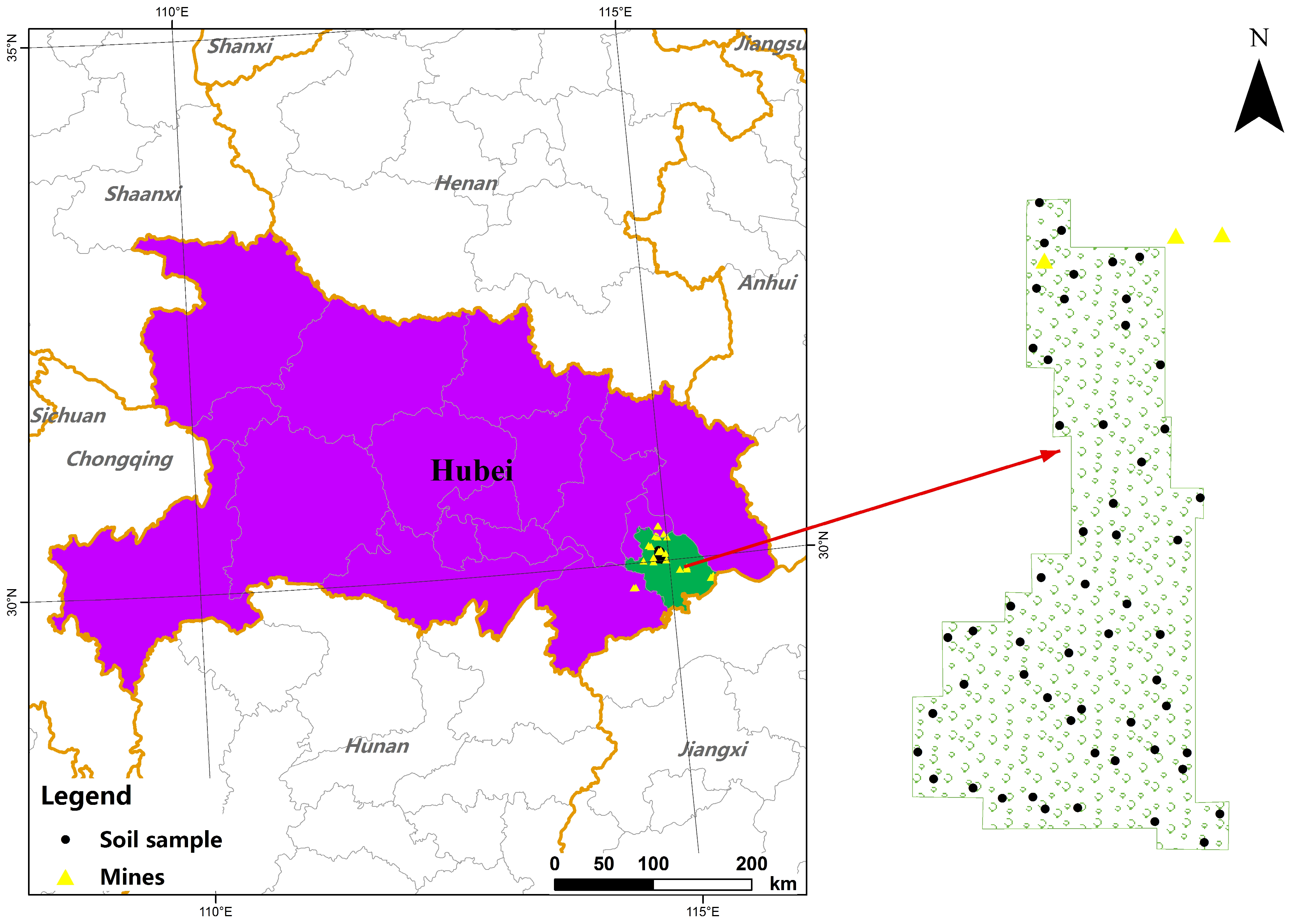
2.1. Study Area and Sampling Points

Daye City, a county-level municipality in Hubei Province, China, is located in the southeastern part of the province on the southern banks of the midstream section of the Yangtze River [42]. It lies between 114°31′ to 115°20′ East longitude and 29°40′ to 30°15′ North latitude (Figure 1). The city is situated on the northern fringes of the hilly terrain of the Mufu Mountains, with a topography that slopes southwards, lowers towards the north, and remains relatively flat in the east and west. The main topographic features include hills, mountains, and plains [25]. With an elevation ranging from 120 to 200 m [12], Daye City has a typical subtropical humid monsoon climate characterized by distinct seasonal changes, abundant sunlight, rainfall, and warmth in each season, and a long frost-free period. The region is known as the birthplace of Chinese bronze culture and possesses a wealth of mineral resources and numerous large- and medium-scale mines. Historical evidence reveals that as early as 3000 years ago, the pioneers of China began Cu mining and smelting in Daye, giving rise to an ancient civilization rich in the art of bronze metallurgy. However, it is important to recognize that these mining and smelting activities have contributed to the contamination of the surrounding soil. Therefore, the agricultural land located in the study area may have the risk of exceeding the Cu content to some extent.

In line with the study area’s characteristics and research objectives, 56 surface soil samples were collected from agricultural land (0–20 cm) surrounding the mining region, with a uniform sampling density of one sample per 500 to 800 m. The detailed sampling strategy for this study can be also found in Figure 1, which was designed to capture the unique characteristics of the study area: The uniform density ensured comprehensive coverage of the study area, allowing for a systematic assessment of Cu distribution throughout the agricultural lands. Such an approach is effective in capturing spatial variations in contamination levels, which can be influenced by factors such as proximity to mining sites, topographical changes, and soil type differences. Given the long history of Cu mining and the presence of numerous mines in the study area, the regions surrounding Cu mine sites were considered high-risk zones for elevated Cu concentrations. By focusing on these regions, the study aimed to assess the impact of both historical and ongoing mining activities on soil Cu levels. Furthermore, uniform sampling is dense enough to capture meaningful variations in Cu levels across the landscape, which also allows for more accurate interpolation between sampling points, thereby providing a more comprehensive understanding of Cu distribution across the entire study area. Lastly, this sampling process ensures that both heavily contaminated and relatively unaffected areas are equally represented in the dataset, providing a more accurate overall demonstration of Cu contamination in the agricultural lands of the study area.

It is noteworthy that the collection, handling, and processing of the soil samples followed the Specification of the Land Quality Geochemical Assessment Standard (DZ/T 0295-2016). The main soil types in the study area are paddy soil and red soil. Each soil sample consisted of three sub-samples, each weighing more than 1000 g. All samples were carefully dried, avoiding exposure to sunlight and moisture. Subsequently, the soil samples were then ground and passed through a 10-mesh nylon screen with a diameter of 2 mm to remove plant residues, rocks, and large debris [12,43]. After the aforementioned processing, those soil samples were then divided into two parts: one for indoor spectral testing and the other for heavy metal measurement in the chemical laboratory.

2.2. Data Determination

A portion of processed soil was sent to the Institute of Geophysical and Geochemical Exploration (IGGE) to assess the soil Cu content. The analysis was performed using plasma mass spectrometry, following the method described in WSBB/001-2019, which allows for the determination of 31 trace elements. The detection limit for Cu in the soil was set at 1.0 $\mathsf{\mu }\mathrm{g}/\mathrm{g}$. Moreover, to ensure the accuracy and reliability of measurement, the laboratory implemented quality control measures by incorporating primary soil reference materials (SRMs) during the analytical process. It is worth noting that the study adhered to the quality requirements established by [44], thus validating the obtained experimental data.

Another portion of processed soil was utilized to acquire soil spectral reflectance using ASD FieldSpec4 spectroradiometers (Analytical Spectral Device, Inc., Boulder, CO, USA). The spectroradiometers covered a wavelength range from 350 to 2500 nm, with a sampling interval of 1.4 nm from 350 to 1100 nm and a 2 nm interval from 1000 to 2500 nm [45]. This level of detail enables the capture of fine spectral features that may be indicative of specific soil characteristics.

To ensure accurate and consistent measurements, great care was taken in preparing the samples and controlling the measurement environment. The soil samples were first screened to remove large particles and ensure homogeneity. They were then placed in clear glass containers with dimensions of approximately 9 cm in diameter and 2 cm in depth. This shallow depth helps to minimize shadowing effects and ensures even illumination across the sample surface. All measurements were conducted in a dark room to eliminate interference from ambient light, providing a controlled environment crucial for precise spectral analysis.

The spectroradiometers were positioned approximately 7 cm above the sample surface and centered over the soil samples, which were evenly distributed in dishes. This consistent positioning is vital for maintaining measurement geometry and ensuring comparable results across all samples. Before taking measurements, a thorough calibration process was followed to ensure the highest possible accuracy. This process began with a 30 min warm-up period to allow the instrument to reach a stable operating temperature. Following this, a sequence of calibration steps was performed, including dark current acquisition to account for internal electronic noise, optimization of instrument settings, and white reference correction to calibrate against a standardized white BaSO₄ panel. The measurements were conducted in a dark room with a stable 50 W halogen lamp as the light source, mounted at a 15° angle and positioned 50 cm away, without any obstructions [12,46]. This setup ensures consistent, even illumination across the sample surface while minimizing specular reflection that could interfere with the diffuse reflectance measurements of interest. For each soil sample, ten individual spectral curves were measured. These multiple measurements were then averaged to reduce random noise and improve the overall signal-to-noise ratio of the data.

After the raw spectral measurements were collected, the data underwent further processing to prepare them for analysis. The averaged spectral curves were subjected to a resampling procedure, resulting in a final output of 2151 spectral bands for each sample, with a consistent interval of 1 nm across the entire measured range. This resampling to a uniform spectral resolution facilitates subsequent data analysis and allows for direct comparison between different soil samples.

Figure 2 presents the measurement results of Cu content and corresponding spectral reflectance for 56 soil samples. From Figure 2a, it is clearly observed that the distribution of Cu content in the soil is highly uneven. Some soil samples show significantly higher Cu content, while others exhibit notably lower levels. As a result, there is a high degree of heterogeneity in the collected soil Cu content. This marked variability may stem from multiple factors, including parent material composition, land-use patterns, environmental pollution levels, and local geological conditions. Figure 2b illustrates that the spectral reflectance and its variation demonstrate complex patterns versus the wavelength. Although the general shape of the spectral curves is similar across all samples, there are evident differences in reflection intensity at various wavelengths. These variations are not solely influenced by Cu content but are likely closely related to other physicochemical properties of the soil, such as organic matter content, particle size distribution, moisture content, and the presence of other minerals. It is the combined effect of these multiple factors that result in such diverse spectral reflectance characteristics.

Given the high heterogeneity of the soil Cu content and the multifaceted factors influencing spectral reflectance, it is difficult, if not impossible, to estimate the soil Cu content from spectra directly. This complexity emphasizes the need to develop a reliable inversion model, coupled with suitable processing methods, for predicting Cu content in the soil. The following sections elucidate the proposed approach in detail.

2.3. Methodology

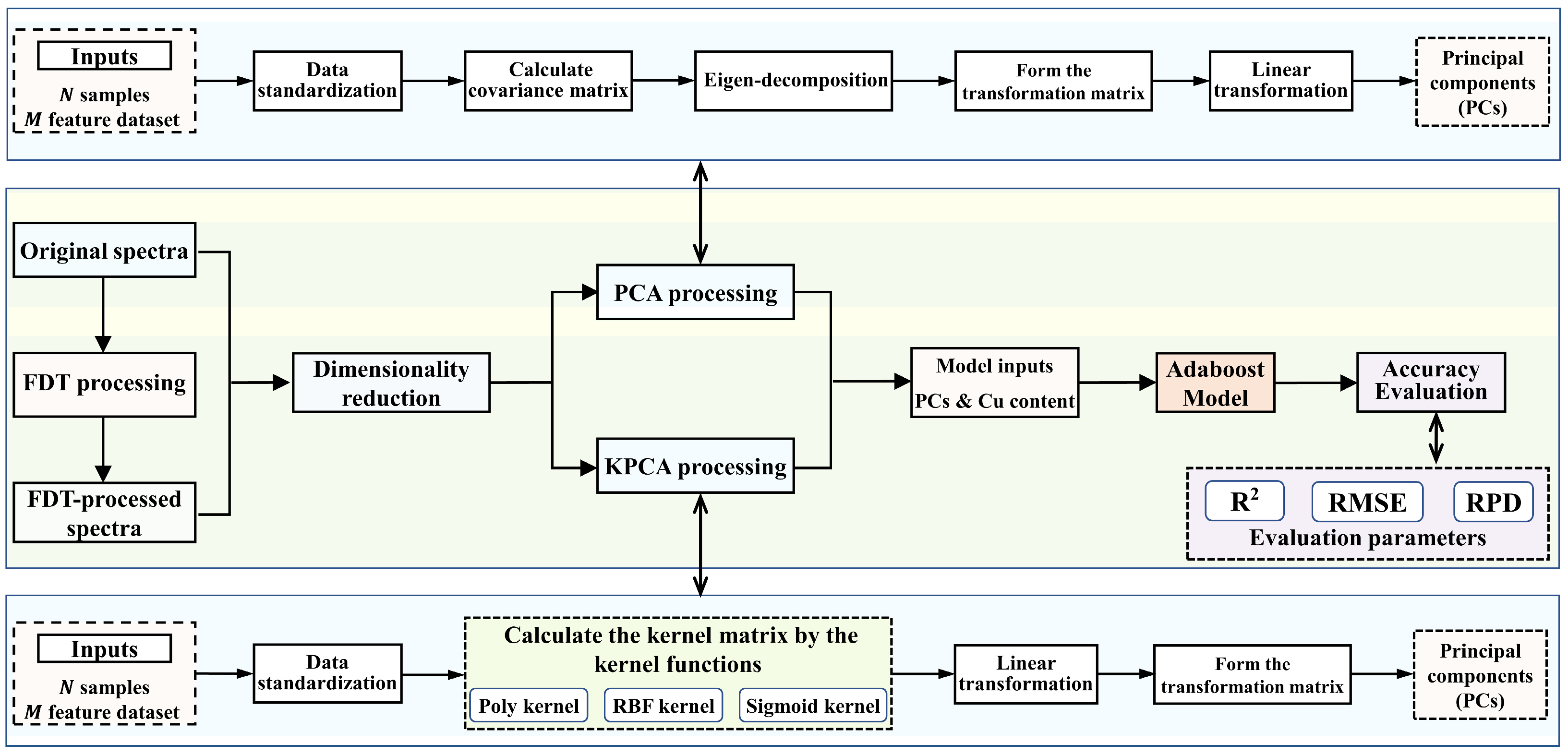
2.3.1. Workflow

The flow chart of this study is depicted in Figure 3. Initially, we proceeded with the spectral reflectance with the FDT processing. Subsequently, we employed both linear and nonlinear dimensionality reduction methods, i.e., the PCA and KPCA, on both the spectral reflectance and that processed by the FDT, wherein the KPCA utilized polynomial, RBF, and sigmoid kernel functions to reduce the dimensionality of the two groups of spectral data (namely the original spectra and FDT-processed spectra). The resulting principal components (PCs) were then used as input variables for inverting the soil Cu content using the PCA/KPCA-AdaBoost-based inversion model. Finally, we investigated the influence of different dimensionality reduction methods on the estimation accuracy for the Cu content to determine the optimal PCA/KPCA-AdaBoost-based inversion model.

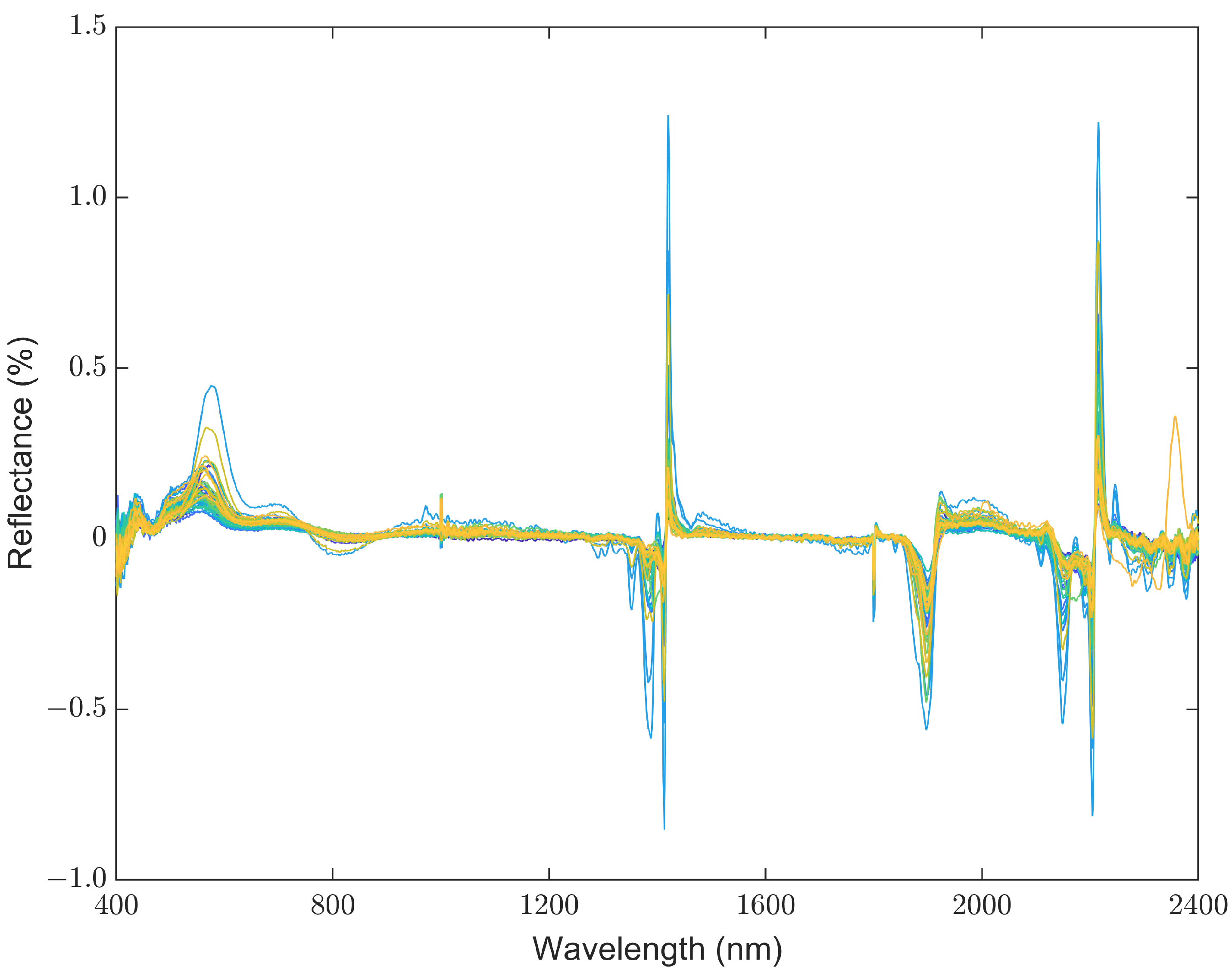
2.3.2. Spectral Pretreatments

In this study, the FDT was employed to preprocess the original spectral data. The FDT could enhance the spectral features by highlighting the regions where the reflectance is changing rapidly with respect to wavelength. The resulting FDT spectra had peaks and valleys that corresponded to the inflection points in the original spectral reflectance. This could help to identify spectral features related to specific soil components or properties. These features were often more pronounced and easier to interpret than the original spectra. Moreover, the FDT was particularly useful for reducing the baseline drifts, background noise, and illumination variations in hyperspectral data, as it is less sensitive to these factors compared to the original reflectance spectra. As a result, the FDT facilitated a more precise identification of characteristic wavelength bands and resulted in a significant improvement in the predictive efficacy of the model [45].

Figure 4 displays the FDT-processed spectral curves of collected soil samples as a function of wavelength, while the corresponding original spectral reflectance is presented in Figure 2. Notably, three prominent absorption peaks, as observed in the vicinity of 1400, 1900, and 2200 nm of FDT processed spectra, are attributable to the absorption properties of soil clay minerals [47,48]. Additionally, it is worth mentioning that wavelengths ranging from 350 to 399 nm and 2450 to 2500 nm were excluded due to their comparatively lower signal-to-noise ratio (SNR) [24]. Consequently, after the removal of these fringe bands, 2050 bands were retained for each sample, thus ensuring the integrity of the analysis.

2.3.3. Spectral Dimensionality Reduction

The PCA is widely adopted for analyzing and streamlining the high-dimensional dataset. The core idea of PCA is to reduce the dimensionality of a dataset comprised of an abundance of interconnected variables while maintaining as much of the original information and variance as possible. In high-dimensional data scenarios, the PCA identifies multiple sets of orthogonal vectors in data space via matrix transformations. This process transforms spectral data, which includes variables with multicollinearity, into a fresh set of uncorrelated variables that form a linear combination of the original independent variables. However, simply increasing the number of PCs does not necessarily yield enhanced results. Typically, the first few PCs can encapsulate a significant portion of the variance in the original dataset. Hence, the selection of preserved PC numbers is generally based on the amount of cumulative variance attributable to the specific portion within the total variance. Nevertheless, the amplification of the preserved PCs can increase the amount of information, but it does not inherently improve the inversion accuracy. Therefore, this study determined the optimal number of preserved PCs based on their impact on the performance of estimating the Cu content. Further, to evaluate the influence of FDT processing on the inversion performance, the PCA was conducted on the original and FDT-processed spectral data.

The KPCA represents a nonlinear approach to data processing that extends the traditional PCA algorithm. Its fundamental concept revolves around projecting the initial data from the input space to a high-dimensional feature space through a nonlinear mapping, typically achieved using kernel functions. The most commonly employed kernel functions include the polynomial (Poly), radial basis function (RBF), and sigmoid kernels. Once the data are mapped to the feature space, KPCA applies the PCA algorithm to compute the PCs by solving an eigenvalue problem using the covariance matrix of the mapped data. This allows KPCA to capture nonlinear relationships in the original data and extract meaningful features. By selecting a subset of the PCs, the KPCA can be used for dimensionality reduction, projecting the data onto a lower-dimensional subspace while preserving the most important nonlinear structures. The kernel functions play a pivotal role in the KPCA algorithm. They furnish a method to implicitly map the input data to a high-dimensional feature space without explicitly computing the coordinates in that space. The kernel functions employed in this study are enumerated as follows.

The polynomial kernel is a kernel function that measures the similarity between two vectors by computing their inner product raised to a specified degree $d$. It serves as a representation of the similarity between these vectors. Essentially, the polynomial kernel takes into account not only the similarity between vectors within the same dimension but also across different dimensions. When employed in machine learning algorithms, this property enables the consideration of feature interaction. The polynomial kernel is defined as follows:

$$k\left(x,y\right)={{(\gamma x}^{T}y+c_0)}^d$$

(1)

where $x$ and $y$ are the input vectors, and $d$is the kernel degree; if $c_0=0$, the kernel is homogeneous.

The RBF kernel function facilitates the computation of the radial basis function (RBF) kernel across a pair of vectors, which is defined as follows:

$$k\left(x,y\right)=\mathrm{e}\mathrm{x}\mathrm{p}{(-\gamma ‖x-y‖}^2)$$

(2)

If $\gamma ={\sigma }^{-2}$, the kernel is known as the Gaussian kernel of variance ${\sigma }^2$.

The sigmoid kernel function facilitates the computation of the sigmoid kernel value, also referred to as the hyperbolic tangent or multilayer perceptron. In neural networks, this kernel is of vital significance, as it commonly serves as an activation function for neurons. We express the sigmoid kernel function as follows:

$$k\left(x,y\right)=\mathit{tanh}{(\gamma x}^{T}y+c_0)$$

(3)

where $\gamma$ is known as slope, and $c_0$ is known as intercept.

Although the parameter optimization could potentially enhance the performance of the KPCA-based inversion model, this study did not conduct specific optimization for the kernel parameters. Instead, the kernel parameters listed in

Table 1. Kernel parameters for the applied kernel functions.

Kernel Functions	Polynomial Kernel	RBF Kernel	Sigmoid Kernel
Kernel parameters	$\gamma ={\displaystyle \frac{1}{n_{\mathrm{f}\mathrm{e}\mathrm{a}\mathrm{t}\mathrm{u}\mathrm{r}\mathrm{e}\mathrm{s}}}}; c_0=1; d=3$	$\gamma ={\displaystyle \frac{1}{n_{\mathrm{f}\mathrm{e}\mathrm{a}\mathrm{t}\mathrm{u}\mathrm{r}\mathrm{e}\mathrm{s}}}}$	$\gamma ={\displaystyle \frac{1}{n_{\mathrm{f}\mathrm{e}\mathrm{a}\mathrm{t}\mathrm{u}\mathrm{r}\mathrm{e}\mathrm{s}}}};c_0=1$

$n_{\mathrm{f}\mathrm{e}\mathrm{a}\mathrm{t}\mathrm{u}\mathrm{r}\mathrm{e}\mathrm{s}}$ represents the number of features for the employed dataset.

were utilized to establish the KPCA-based inversion models to ensure the generalizability of each inversion model while maintaining comparability across different models.

2.3.4. Model Construction

Boosting is a powerful ensemble learning algorithm for both classification and regression problems, which iteratively updates the weights of the base classifiers based on changes in sample weights, resulting in a high-performance model [29]. Among its variants, AdaBoost stands out as one of the most successful algorithms that has resolved numerous practical issues [49]. In this study, AdaBoost was utilized to invert Cu content in the soil. Some of the potential benefits of using the AdaBoost algorithm in this context include improved accuracy by combining multiple weak learners, robustness to noise, the ability to capture non-linear relationships, and a degree of interpretability through the individual weak learners used in the ensemble [50]. Further, the AdaBoost method is less prone to overfitting and has fewer parameters, reducing the need for extensive parameter tuning in applications. Since the AdaBoost model does not limit the types of weak learners, different learning algorithms can be used to construct weak classifiers. Moreover, compared to the bagging algorithm and random forest algorithm, AdaBoost fully considers the weight of each classifier, leading to high accuracy. A step-by-step procedure of the AdaBoost algorithm is summarized in Algorithm 1.

Algorithm 1. The procedure outline for the AdaBoost algorithm

1. Initialize sample weights Assign equal weights to all training samples, typically initialized as 1/N, where N is the total number of samples.

2. For each iteration t = 1, 2,..., T (1) Train a weak classifier: Fit a weak classifier (e.g., decision stump or decision tree) to the training data, taking into account the sample weights, to minimize the weighted classification error. (2) Calculate the weighted error of the weak classifier: Compute the weighted error ${\mathsf{\epsilon }}_{\mathrm{t}}$ by summing the weights of the misclassified samples, with ${\mathsf{\epsilon }}_{\mathrm{t}}=\mathsf{\Sigma }\left({\mathrm{w}}_{\mathrm{i}}\ast \mathrm{I}\left({\mathrm{y}}_{\mathrm{i}}\ne {\mathrm{h}}_{\mathrm{t}}\left({\mathrm{x}}_{\mathrm{i}}\right)\right)\right)$, where ${\mathrm{w}}_{\mathrm{i}}$ is the weight of sample $i$, $I\left(\right)$ is the indicator function, ${\mathrm{y}}_{\mathrm{i}}$ is the true label, and ${\mathrm{h}}_{\mathrm{t}}\left({\mathrm{x}}_{\mathrm{i}}\right)$ is the predicted label by the weak classifier. (3) Compute the coefficient ${\alpha }_t$ for the weak classifier: ${\alpha }_t=0.5\ast ln\left(\left(1-{\epsilon }_t\right)/{\epsilon }_t\right)$, where $ln\left(\right)$is the natural logarithm, and ${\alpha }_t$ represents the importance or weight of the weak classifier in the final ensemble. (4) Update the sample weights: Increase the weights of the misclassified samples and decrease the weights of the correctly classified samples. $$\begin{gathered} {\mathrm{w}}_{\mathrm{i}}={\mathrm{w}}_{\mathrm{i}}·\mathrm{e}\mathrm{x}\mathrm{p}\left\{{\mathsf{\alpha }}_{\mathrm{t}}·\mathrm{I}\left(\left[{\mathrm{y}}_{\mathrm{i}}\ne {\mathrm{h}}_{\mathrm{t}}\left({\mathrm{x}}_{\mathrm{i}}\right)\right]\right)\right\} \mathrm{for} \mathrm{misclassified} \mathrm{samples}. \\ {\mathrm{w}}_{\mathrm{i}}={\mathrm{w}}_{\mathrm{i}}·\mathrm{e}\mathrm{x}\mathrm{p}\left(-{\mathsf{\alpha }}_{\mathrm{t}}·\mathrm{I}\left({\mathrm{y}}_{\mathrm{i}}={\mathrm{h}}_{\mathrm{t}}\left({\mathrm{x}}_{\mathrm{i}}\right)\right)\right) \mathrm{for} \mathrm{correctly} \mathrm{classified} \mathrm{samples}. \end{gathered}$$ (5) Normalize the sample weights: Normalize the updated weights so that they sum up to 1. $${\mathrm{w}}_{\mathrm{i}}={\mathrm{w}}_{\mathrm{i}}/\mathsf{\Sigma }\left({\mathrm{w}}_{\mathrm{i}}\right) \mathrm{for} \mathrm{all} \mathrm{samples}.$$

3. Combine the weak classifiers: The final AdaBoost classifier $H\left(x\right)$ is a weighted combination of all weak classifiers. $$\mathrm{H}\left(\mathrm{x}\right)=\mathrm{s}\mathrm{i}\mathrm{g}\mathrm{n}\left(\mathsf{\Sigma }\left({\mathsf{\alpha }}_{\mathrm{t}}\ast {\mathrm{h}}_{\mathrm{t}}\left(\mathrm{x}\right)\right)\right),$$ where $\mathrm{s}\mathrm{i}\mathrm{g}\mathrm{n}\left(\right)$ is the sign function that returns +1 and −1 for positive and negative values, respectively.

4. Make predictions (1) For a new input sample $x$, compute the predictions of all the weak classifiers. (2) Combine the predictions using the weighted sum: $\mathsf{\Sigma }\left({\mathsf{\alpha }}_{\mathrm{t}}\ast {\mathrm{h}}_{\mathrm{t}}\left(\mathrm{x}\right)\right)$. (3) Apply the sign function to obtain the predicted class label: $\mathrm{s}\mathrm{i}\mathrm{g}\mathrm{n}\left(\mathsf{\Sigma }\left({\mathsf{\alpha }}_{\mathrm{t}}\ast {\mathrm{h}}_{\mathrm{t}}\left(\mathrm{x}\right)\right)\right)$.

The AdaBoost algorithm iteratively trains weak classifiers, assigns them weights based on their performance, and updates the sample weights to focus on the misclassified samples. The final classifier is a weighted combination of all the weak classifiers, where weights are determined by their individual accuracies. By following the aforementioned procedure, AdaBoost creates a strong classifier that can effectively classify new samples based on the combined predictions of the weak classifiers.

2.3.5. Accuracy Validation

To evaluate the estimation performance and predictive accuracy of the inversion models for Cu content in the soil, three evaluation metrics in terms of the coefficient of determination (R²), root-mean-square error (RMSE), and residual prediction deviation (RPD) were utilized. These metrics are commonly adopted in similar studies, where R² measures the proportion of variance in the dependent variable that is predictable from the independent variables; RMSE provides the standard deviation of the prediction errors or residuals, offering a measure of how far the predicted values are from the observed values; and RPD is the ratio of the standard deviation of the observed values to the RMSE [8,51]. The representations for these evaluation metrics are presented below:

$${\mathrm{R}}^2=1-{\displaystyle \frac{\sum _{i=1}^n{\left(y_i-{\widehat{y}}_i\right)}^2}{\sum _{i=1}^n{\left(y_i-{\overline{y}}_i\right)}^2}}$$

(4)

$$\mathrm{R}\mathrm{M}\mathrm{S}\mathrm{E}=\sqrt{{\displaystyle \frac{1}{n}}\sum _{i=1}^n{\left({\widehat{y}}_i-y_i\right)}^2}$$

(5)

$$\mathrm{R}\mathrm{P}\mathrm{D}={\displaystyle \frac{\mathrm{S}\mathrm{D}}{\mathrm{R}\mathrm{M}\mathrm{S}\mathrm{E}}}$$

(6)

where $y_i$ and ${\widehat{y}}_i$ represent measured and predicted content separately of samples in the validation set, ${\overline{y}}_i$ represents the mean of samples, $n$ represents the number of samples, and $\mathrm{S}\mathrm{D}$ represents the standard deviation of samples. It should be noted that both the coefficient of determination and RPD are dimensionless metrics, whereas the RMSE is expressed in the same unit as the measured Cu content, i.e., mg·kg⁻¹ in this case.

Generally, a robust model is characterized by high R² and RPD but by a low RMSE. R² and RPD are frequently used to evaluate the accuracy of inversion performance, while the RMSE is dependent on the range of measured values [52,53]. The interpretation of these metrics is as follows:

(1)

R² is a measure of the proportion of the variance in the dependent variable that is predictable from the independent variable (s). An R² value close to 1 indicates a high goodness of fit, while a value close to 0 suggests a poor fit;

(2)

RMSE represents the standard deviation of the prediction residuals and provides a measure of the average magnitude of the errors. A lower RMSE indicates a better model fit;

(3)

An RPD value greater than 2.0 indicates an excellent inversion performance. An RPD value between 1.4 and 2.0 suggests the ability to distinguish between high and low values. An RPD value less than 1.4 represents an unsuccessful inversion performance.

3. Results

3.1. Statistic Analysis of Cu Content in Soil

The soil samples were divided into two groups: 38 samples for calibration and 18 samples for validation.

Table 2. Statistical descriptions of soil Cu content (mg·kg⁻¹).

Soil Cu (mg·kg−1)	Number	Min	Max	Median	Mean	SD 1	CV 2
Calibration set	38	21.68	320.86	73.03	90.43	67.89	0.75
Validation set	18	29.81	284.73	73.38	86.10	58.36	0.68
Whole dataset	56	21.68	320.86	73.03	89.04	64.48	0.72

¹ SD: standard deviation; ² CV: coefficient of variation.

provides a statistical summary of the soil Cu content characteristics. As seen, the overall dataset revealed an average Cu content of 67.89 mg/kg. This average exceeds that of the validation subset but is less than the calibration subset’s mean. It is noteworthy that the natural background level of soil Cu content, as reported in the China Soil Elements Background Values by the China National Environmental Monitoring Centre, is 92 mg/kg. Significantly, 21.4% of the samples surpassed the national pollution threshold levels. Furthermore, the highest observed Cu content exceeded the natural background level, and a coefficient of variation above 0.72 indicates a considerable spatial variability in the Cu content distribution across the study area.

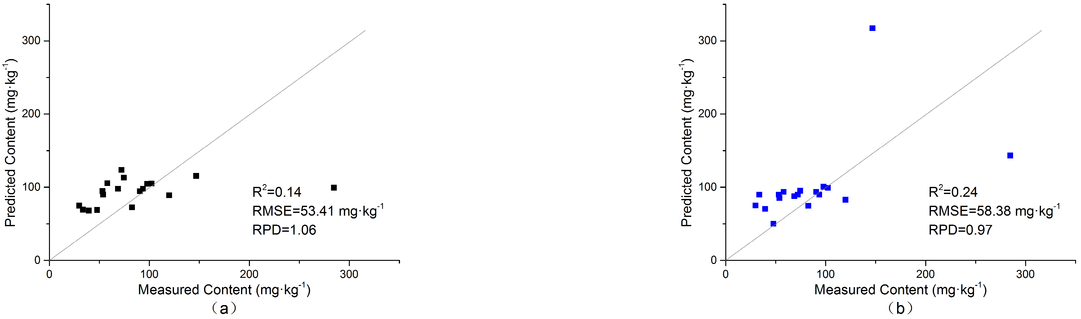
3.2. Inversion Accuracy without Dimensionality Reduction

Before applying the dimensionality reduction in terms of PCA and KPCA processing, we should first focus on the hyperspectral inversion performance using the spectral data without applying any dimensionality reductions. To this end, the AdaBoost-based inversion models were established in accordance with the original and FDT-processed spectra. The corresponding results are presented in Figure 5 and serve as the baseline for comparison with the following dimensionality reduction methods (PCA and KPCA).

The results in Figure 5 reveal notable differences between the performance when using the original spectra versus the FDT-processed spectra for predicting Cu content in the soil. The inversion model based on the original spectra displayed a limited predictive performance, as evidenced by a minor R² value of 0.14. This subpar performance may be attributed to the presence of substantial noise and interferents in the original spectra, which hindered the ability of the inversion model to capture the underlying relationship between the spectral features and Cu contents. In contrast, the inversion model constructed using the FDT-processed spectra showed an improved R² of 0.24, suggesting that the FDT preprocessing was effective in removing unwanted noise and enhancing the informative spectral features for Cu content prediction but to a limited extent.

Nonetheless, it is worth noting that neither the original spectra nor FDT-processed spectra achieved a desirable coefficient of determination. Furthermore, the RPD values in both cases were consistently below 1.4, signifying an overall inadequate performance in inverting soil Cu content. These unsatisfactory results underscore the significance of employing dimensionality reduction, such as PCA and KPCA, in this particular spectral analysis pertaining to Cu content. The diminished R² values hint at the possibility of redundant or irrelevant features within the raw spectral data, impeding the model’s predictive capability. By implementing PCA and KPCA to extract the most informative principal components or nonlinear features, it is anticipated that subsequent inversion models may attain enhanced performance. This dimensionality reduction step can aid in noise filtration, multicollinearity elimination, and the identification of key spectral signatures that exhibit the highest correlation with Cu content. Further details are expounded upon below.

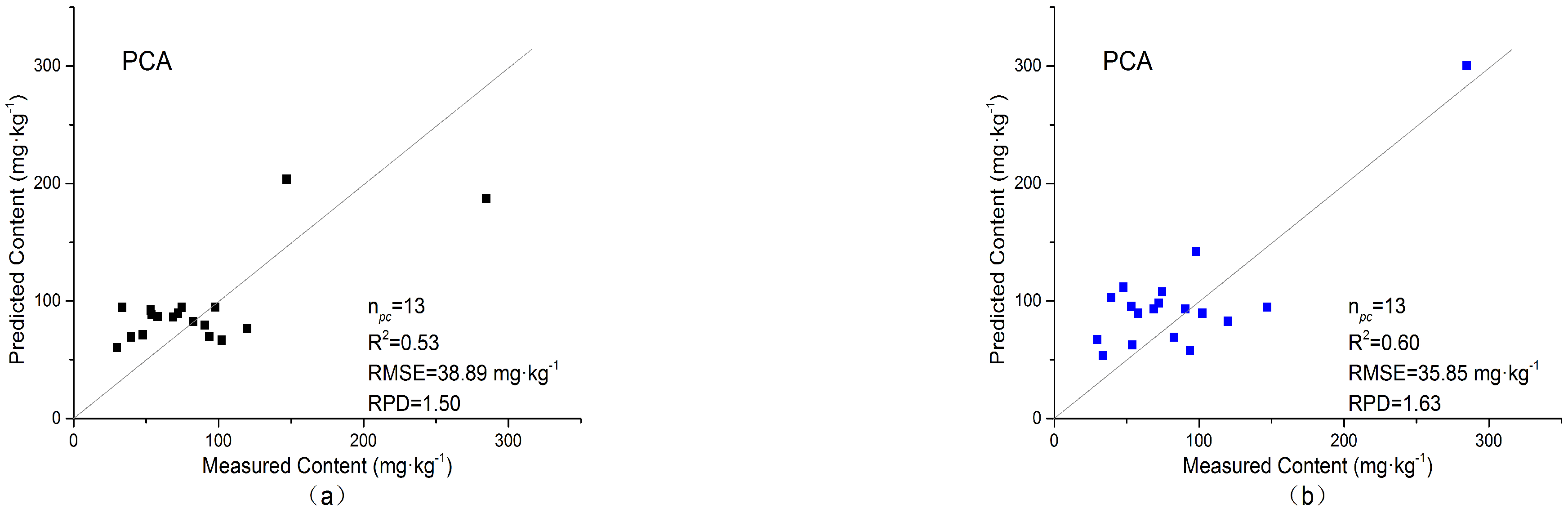
3.3. Inversion Accuracy with PCA Processing

Next, the AdaBoost-based model for inverting the Cu content was developed with the PCA-processed spectra. The independent variables of the inversion model were the preserved PCs obtained after applying PCA to the original and FDT-processed spectra, while the dependent variables were the soil Cu content. On this foundation, a comparative analysis of the inversion performance under different numbers of PCs was conducted to determine the optimal number of preserved PCs. The methodology for selecting the optimal number of principal components in PCA/KPCA-based inversion models was as follows:

(1)

Cumulative explained variance: The individual and cumulative explained variance of the PCs were first calculated. This process was continued until the cumulative explained variances reached 99.99%, which resulted in a large number of potential PCs;

(2)

Iterative model building and evaluation: Starting with the first PC, we incrementally built inversion models using an increasing number of principal components (1 to $n$, where $n$ is the number of PCs needed to reach 99.99% cumulative explained variance). For each iteration, we used the current set of PCs as input variables for the Cu inversion model and evaluated the performance using metrics in terms of ${\mathrm{R}}^2$, PRD, and RMSE;

(3)

Optimal selection: By comparing the inversion accuracy across all established inversion models, we determined the number of PCs that resulted in the highest accuracy (lowest RMSE, highest R², or highest RPD) as the optimal choice.

The aforementioned methodology balances the need to retain sufficient information, and it allows for data-driven decision making rather than arbitrary cutoffs. Furthermore, this approach considers both the explained variance and mode performance while avoiding overfitting. The results suggest that using all preserved PCs corresponding to 99.99% cumulative explained variances as input variables did not always lead to the best inversion results. The underlying reason for this is that as the number of preserved PCs increased, noise was introduced into the inversion model to a certain extent.

The inversion results from using the optimal preserved PCs are presented in Figure 6, and the validation outcomes of the AdaBoost-based inversion models are also illustrated in Figure 6.

The results in Figure 6 reveal the PCA-AdaBoost-based inversion model achieved the optimal predictive accuracy, regardless of using original or FDT-processed spectra, when 13 preserved PCs were employed. Additionally, the results indicate that FDT processing can enhance the performance of the PCA-AdaBoost-based inversion model to a certain extent. Specifically, the model with FDT processing yielded an R² of 0.60, an RMSE of 35.53 mg·kg⁻¹, and an RPD of 1.63, respectively. In contrast, the AdaBoost-based inversion model with the original spectra exhibited inferior performance, with the corresponding R², RMSE, and RPD values being 0.53, 38.89 mg·kg⁻¹, and 1.53, respectively. The overall results indicate that the inversion model employing PCA processing exhibited inferior performance for estimating the Cu content, suggesting that the linear dimensionality reduction method is unable to effectively capture the nonlinear relationship between the spectral data and Cu content, thereby leading to suboptimal predictive performance.

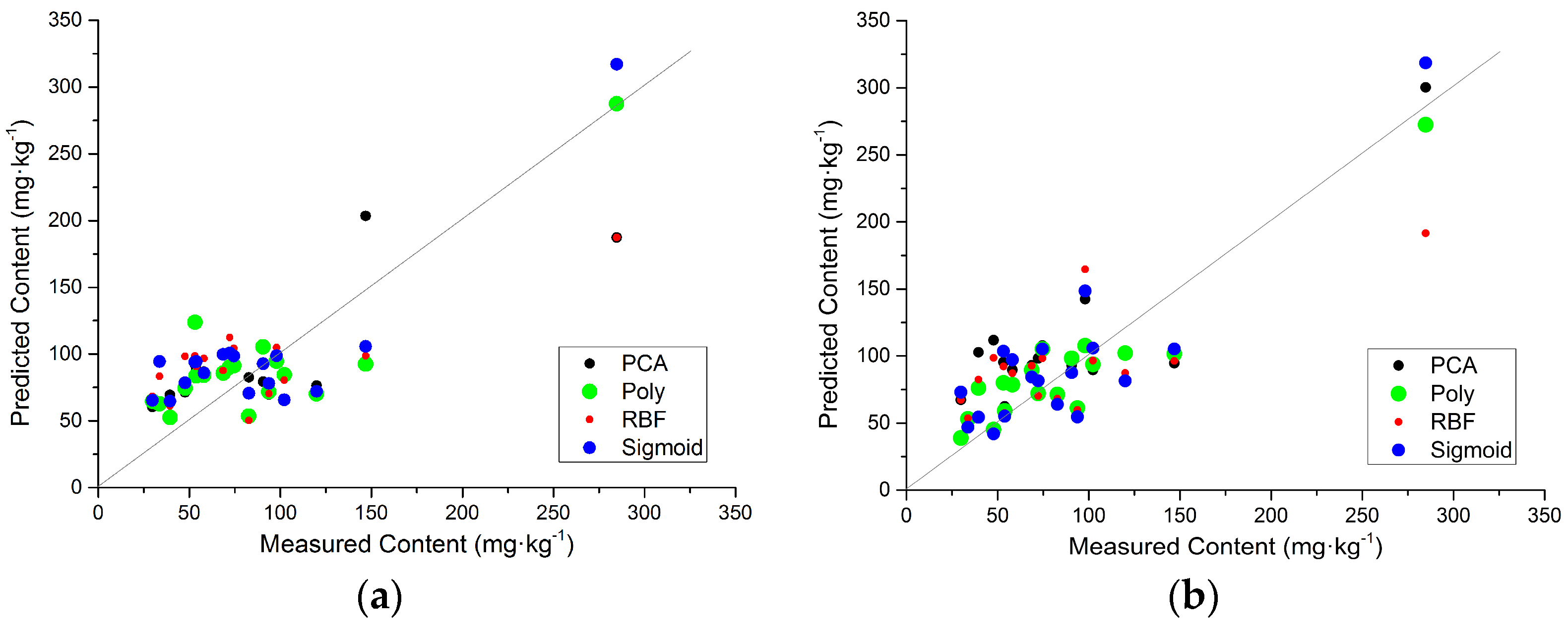
3.4. Inversion Accuracy of KPCA Dimensionality Reduction Methods

KPCA is a powerful methodology for non-linear dimensionality reduction. In this study, we implemented three distinct kernel functions to effectively reduce the dimensionality of both the original and FDT-processed spectral data. Subsequently, we estimated the Cu content using the obtained data and proceeded to compare the corresponding accuracies. The detailed analysis results are provided in the following.

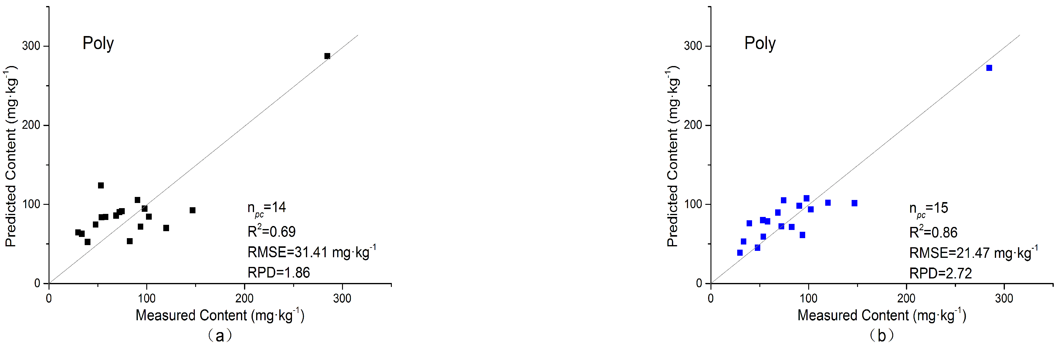
3.4.1. Polynomial Kernel

The implementation of a polynomial kernel was employed in KPCA to reduce the dimensionalities of both the original and FDT-processed spectral data. Subsequently, distinct preserved PCs were utilized as input variables of the AdaBoost-based inversion model to invert Cu content. Then, a comparison was made across the achieved inversion accuracies. The evaluation results, obtained under the optimal number of principal components, are presented in Figure 7. Furthermore, the estimation results of the inversion model considering different spectral types are also illustrated in Figure 7.

From Figure 7, it is evident that the utilization of 14 preserved PCs resulted in optimal prediction accuracy when using the original spectral dataset. On the other hand, in the case of the FDT-processed spectra, the inversion accuracy reached its peak with the utilization of 15 preserved PCs. It is noteworthy that the FDT processing could significantly enhance the predictive capability. The respective values of R², RMSE, and RPD for the KPCA-AdaBoost-based inversion model improved from 0.69, 31.41 mg·kg⁻¹, and 1.86 for the original spectral case to 0.86, 21.47 mg·kg⁻¹, and 2.74 for the FDT-processed spectral case.

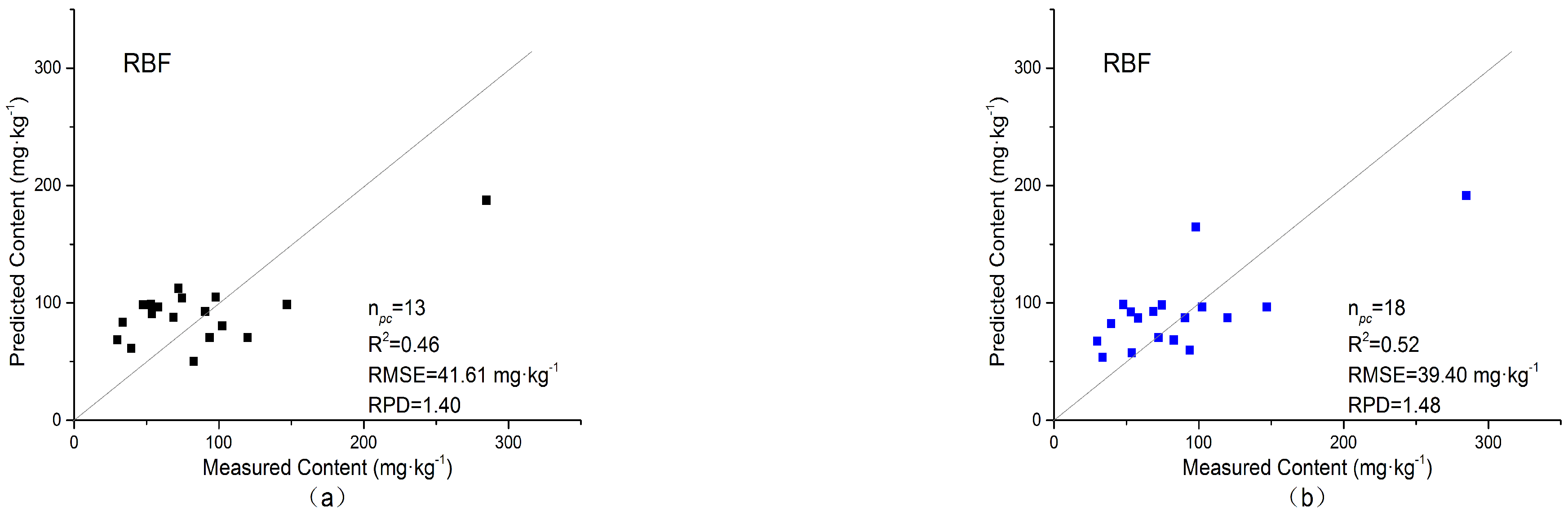
3.4.2. RBF Kernel

When the spectral dimensionality was reduced by KPCA utilizing the RBF kernel function, the subsequent accuracy of its prediction under the optimal preserved PCs was achieved as is presented in Figure 8. To further visualize the relationship between the estimated soil Cu content and the measured Cu content, we refer to Figure 8, which showcases a scatterplot.

Both results in Figure 8 demonstrate that the performance of the inversion model with the RBF kernel is not at an ideal level, though the FDT processing continues to improve inversion results to some extent. Specifically, within the AdaBoost-based inversion model, the utilization of the original spectra, accompanied by 13 principal components, resulted in an optimal R² of 0.46, an RMSE of 41.61 mg·kg⁻¹, and an RPD of 1.40. By contrast, when employing the FDT-processed spectra, it was found that the most beneficial PCs to retain were the first 18 ones. This refinement led to an enhancement in the accuracy of the inversion model, resulting in evaluation indices of 0.52, 39.4 mg·kg⁻¹, and 1.48.

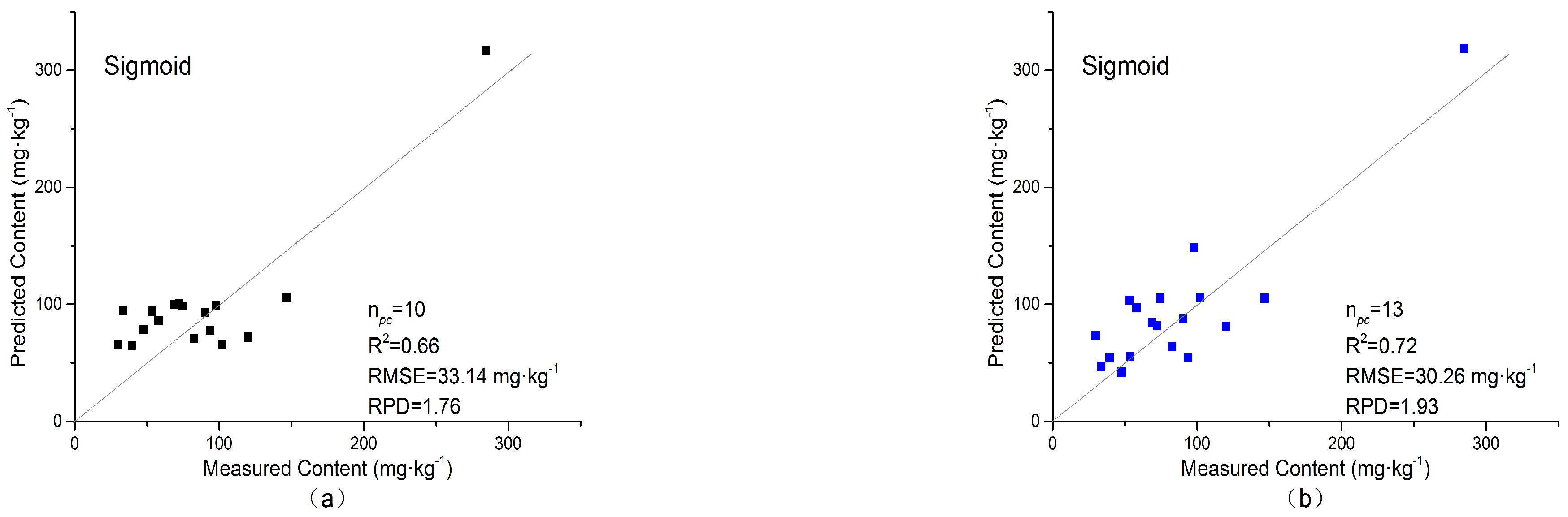
3.4.3. Sigmoid Kernel

Next, the sigmoid kernel was employed to reduce the dimensions of both the original and FDT-processed spectra. Subsequently, we scrutinized the performance of the KPCA-AdaBoost-based inversion model in estimating the Cu content. The results show that the number of optimal preserved PCs varied according to the spectral type. The optimal preserved PC and corresponding evaluation are presented in Figure 9, while Figure 9 visually illustrates the scatterplot of estimated Cu content versus the measured Cu content.

The results in Figure 9 suggest that for the original spectra, the application of 10 preserved PCs yielded the optimal inversion performance. The corresponding R², RMSE, and RPD values were 0.66, 33.14 mg·kg⁻¹ and 1.76, respectively. Conversely, the inversion model utilizing the FDT-processed spectra surpassed that using original spectra in terms of estimation accuracy, demonstrating a noteworthy improvement. This enhancement was achieved by effectively incorporating 13 preserved PCs, resulting in evaluation indices of 0.72 (R²), 30.26 mg·kg⁻¹ (RMSE), and 1.93 (PRD), respectively.

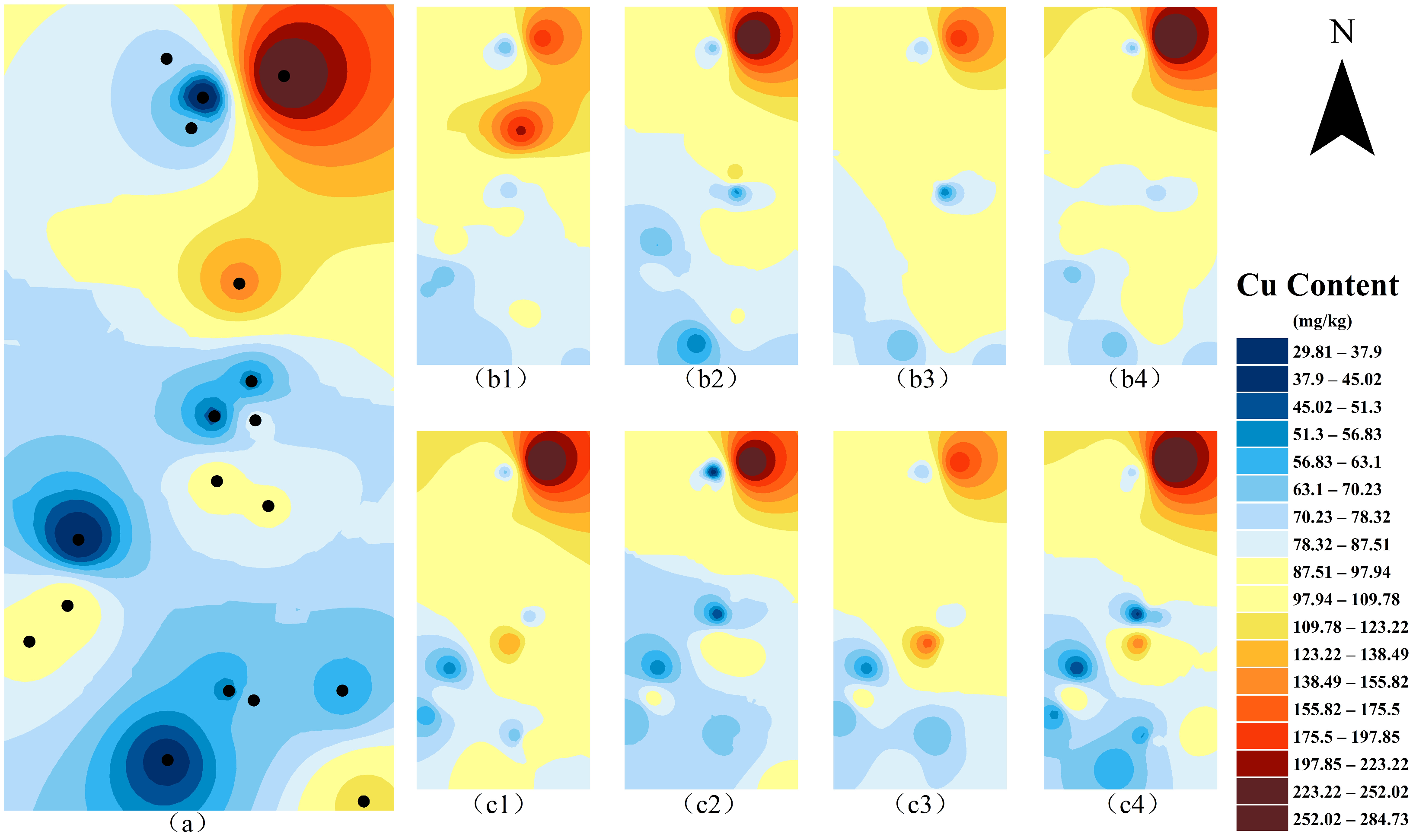
3.5. Spatial Distribution of Soil Cu Contents

Geostatistics, grounded in the theory of regionalized variables, is pivotal for revealing spatial structures. In the field of soil science, a primary application of geostatistics involves estimating and mapping soil attributes in unsampled regions. In this study, the inverse-distance weighting (IDW) method, a prototypical algorithm in geostatistics, is employed to delineate the spatial arrangement and variability of Cu content. This preference is attributable to its computational efficiency and straightforward implementation [54,55].

Figure 10 depicts the spatial distribution of Cu content within the study area, mapped and simulated using the IDW method. It contrasts the experimental chemical analysis values of Cu with the predicted values from both original and FDT processed spectra, employing various dimensionality reduction techniques within the AdaBoost-based inversion model. While the geochemical maps of all predicted values mirror the general trend of the interpolated measured values, notable deviations are observed in Figure 10b1,b3,c3 within the high-value zone (223.22 to 284.73 mg/kg). Similarly, slight differences are evident in the low-value zone (29.81 to 45.02 mg/kg), especially in Figure 10b1,b3,b4,c1. The comparative analysis in Figure 10c2 highlights the closest resemblance to the geochemical maps of the measured values. Furthermore, the spatial distribution analysis of soil Cu content suggests that areas with notably high Cu levels are predominantly located in the northeastern section of the study area. This enrichment trend exceeds the benchmarks set by the China Soil Elements Background Values. On the other hand, the southern and southwestern regions of the study area are characterized by comparatively low Cu concentrations.

4. Discussion

The precision of hyperspectral inversion for the soil Cu content is influenced not only by the spectral preprocessing but also by dimensionality reduction method [56,57,58,59,60,61,62]. A suitable combination of spectral preprocessing and dimensionality reduction can improve the accuracy and performance of the inversion model. Moreover, prior research has indicated that fine-tuning the number of preserved PCs can contribute to improving the performance of the inversion model when applying PCA and its variants [56,57,58].

In this study, both the original and FDT-processed spectra were subjected to PCA/KPCA processing to serve as input variables. On this foundation, the AdaBoost-based inversion model then leveraged these inputs at the optimal PC count to estimate soil Cu content. The rationale behind this approach was to analyze the impact of linear dimensionality reduction methods and the non-linear dimensionality reduction method in terms of KPCA with various kernel functions on the estimation performance of Cu content. The performances of these inversion models were evaluated using R², RMSE, and RPD metrics, as shown in

Table 3. The prediction accuracies of the AdaBoost-based inversion models under the original and FDT-processed spectra.

Methods	Spectral Type	The Number of Optimal Preserved PCs	Prediction Accuracy
			R2	RMSE (mg·kg−1)	RPD
Non-dimensionality reduction	Original spectra	-	0.14	55.41	1.06
	FDT-processed spectra	-	0.24	58.38	0.97
PCA	Original spectra	13	0.53	38.89	1.50
	FDT-processed spectra	13	0.60	35.85	1.63
Poly-KPCA	Original spectra	14	0.69	31.41	1.86
	FDT-processed spectra	15	0.86	21.47	2.72
RBF-KPCA	Original spectra	13	0.46	41.61	1.40
	FDT-processed spectra	18	0.52	39.40	1.48
Sigmoid-KPCA	Original spectra	10	0.66	33.14	1.76
	FDT-processed spectra	13	0.72	30.26	1.93

. Additionally, Table 3 underscores the optimal number of preserved PCs for different spectra and dimensionality reduction methods that led to enhanced inversion accuracy. The scatter plots summarizing the performance of all inversion models are presented in Figure 11.

Different dimensionality reduction methods (PCA and KPCA with various kernels) corresponded to different numbers of optimal preserved PCs. For example, under the original spectra, the optimal number of PCs was 13 for the PCA, while it was 10 for the RBF-KPCA. Moreover, the FDT processing could affect the number of optimal PCs to a certain extent. Taking PCA as an example, the optimal number of PCs was 13 under the original spectra, but it increased to 15 after FDT processing, while other KPCA methods also showed similar changes. Thus, it could be concluded the choice of dimensionality reduction method and spectral preprocessing both influence the optimal number of PCs.

The prediction performance varies significantly among different dimensionality reduction methods: When employing the PCA processing for dimensionality reduction, the performance of the inversion model did not meet expectations regardless of whether original or FDT-processed spectra were used. This result suggested that while inversion models employing PCA for dimensionality reduction have some predictive power, there is room for further optimization. Interestingly, the inversion model’s accuracy was enhanced when FDT-processed spectra were applied, suggesting the FDT preprocessing step may be enhancing certain spectral features that are beneficial for the AdaBoost-based inversion model.

The PCA processing was not fully able to meet the precision requirements of a satisfied inversion model, largely due to the non-linear relationship between the measured spectral data and Cu content. The PCA is a linear method of reducing dimensionality that identifies the preserved PCs of the data [59,60]. Hence, it could not yield optimal results with non-linear relation data. In contrast, KPCA allows to effectively manage non-linear relationships by the kernel functions [61]. Thus, the efficacy of KPCA is significantly dependent on the selection of the kernel function, as different kernel functions are appropriate for different types of data, thereby leading to varied inversion outcomes [62].

In this study, three kernel functions, namely polynomial, RBF, and sigmoid kernels, were employed, and the corresponding inversion performances under original and FDT-processed spectra were evaluated. A comparative analysis aimed to identify the most effective dimensionality reduction method for the study area’s data. Under the original spectra, RBF-KPCA achieved the highest R² of 0.69, outperforming other methods. Through this comparative study, we also discovered that the FDT-processed spectra could significantly improve the accuracy of the inversion model in contrast to the original spectral data. After FDT processing, the inversion model with Poly-KPCA processing reached an R² of 0.86, yielding the best prediction results, as detailed in Table 3. As a result, the dimensionality reduction achieved by KPCA-Poly, in conjunction with the FDT-processed spectra, demonstrated exceptional estimation performance in the AdaBoost-based inversion model, with an R² of 0.86 and an RPD of 2.72. Such high evaluation values indicate that the model’s validation accuracy is exceptionally predictive. This indicates that selecting appropriate data processing methods is crucial for improving model performance for specific problems.

The Poly-KPCA-AdaBoost-based inversion model showed excellent capability in estimating soil Cu content using FDT-processed spectra in the study area. Nevertheless, further exploration is warranted to enhance the proposed model. A key limitation of the inversion model stems from the vast array of intricate variables that impact the accuracy of inversion. Factors such as soil composition, color, type, and the levels of individual soil elements have diverse impacts on the spectral data, thus affecting the precision of the inversion model. Moreover, the model’s inversion accuracy depends on several factors, including the spectral measurement, element measurement, spectral preprocessing, etc. Therefore, our future research will investigate the transferability of the proposed inversion model to fully assess its capabilities and broaden its practical use.

5. Conclusions

This study investigated the effects of the PCA and KPCA with polynomial, RBF, and sigmoid kernels on the inversion performance of Cu content using the spectral data. To this end, both original and FDT-processed spectral data were utilized for dimensionality reduction. Using these two groups of spectral data as inputs, the AdaBoost-based inversion models were established, and the hyperspectral inversion was conducted by the proposed model. Comparing inversion results under various dimensionality reduction methods, it was found that the polynomial kernel function can enhance the feature extraction, which, in effect, yields the optimal inversion performance for the soil Cu content. Moreover, the FDT processing could substantially improve the accuracy of the inversion model. As a result, the performance of the inversion model based on the transformed spectra surpassed that based on original spectra, indicating the effectiveness of spectral transformation in mitigating noise, varying backgrounds, and baseline interference. Ultimately, when employing the spectral data processed by FTD and KPCA with the polynomial kernel, the AdaBoost-based inversion model achieved the optimal accuracy at 15 preserved PCs, with R² and RPD values being 0.86 and 2.72, respectively.

The results highlight the substantial potential of soil spectral analysis for estimating the soil Cu content and monitoring the spatial distribution of heavy metal contamination. In contrast to the conventional land-quality survey, the soil spectral analysis offers advantages in terms of time and manpower. Therefore, future research should focus on further exploring the inversion of heavy metal contents based on soil spectral analysis, particularly investigating the feasibility of using field spectral measurements to estimate element contents and assessing the model’s transferability across different environments.

References

- Liu, X.Y.; Bai, Z.K.; Shi, H.D.; Zhou, W.; Liu, X.C. Heavy metal pollution of soils from coal mines in China. Nat. Hazards 2019, 99, 1163–1177. [Google Scholar] [CrossRef]
- Liu, Y.; Du, Q.Y.; Cheng, Z.H.; Chen, J.W.; Lin, Z.J. Generation Model of Optimal Emergency Treatment Technology for Sudden Heavy Metal Pollution Based on Group-G1 Method. Pol. J. Environ. Stud. 2021, 30, 5899–5908. [Google Scholar] [CrossRef]
- Qi, D. Accumulation Effect of Heavy Metal Cadmium by Immobilization Microorganism. Master’s Thesis, Shanxi University, Taiyuan, China, 2010. [Google Scholar]
- Meng, W.; Shanshan, L.I.; Xiaoyue, L.I.; Zhongqiu, Z.; Shibao, C. An overview of current status of copper pollution in soil and remediation efforts in China. Earth Sci. Front. 2018, 25, 305–313. [Google Scholar]
- Rattan, R.K.; Patel, K.P.; Manjaiah, K.M.; Datta, S.P. Micronutrients in Soil, Plant, Animal and Human Health. J. Indian Soc. Soil Sci. 2009, 57, 546–558. [Google Scholar]
- Sun, W.; Zhang, X.; Sun, X.; Sun, Y.; Cen, Y. Predicting nickel concentration in soil using reflectance spectroscopy associated with organic matter and clay minerals. Geoderma 2018, 327, 25–35. [Google Scholar] [CrossRef]
- Khosravi, V.; Doulati Ardejani, F.; Yousefi, S.; Aryafar, A. Monitoring soil lead and zinc contents via combination of spectroscopy with extreme learning machine and other data mining methods. Geoderma 2018, 318, 29–41. [Google Scholar] [CrossRef]
- Wang, J.; Cui, L.; Gao, W.; Shi, T.; Chen, Y.; Gao, Y. Prediction of low heavy metal concentrations in agricultural soils using visible and near-infrared reflectance spectroscopy. Geoderma 2014, 216, 1–9. [Google Scholar] [CrossRef]
- Kemper, T.; Sommer, S. Estimate of heavy metal contamination in soils after a mining accident using reflectance spectroscopy. Environ. Sci. Technol. 2002, 36, 2742. [Google Scholar] [CrossRef]
- Jarmer, T.; Vohland, M.; Lilienthal, H.; Schnug, E. Estimation of some chemical properties of an agricultural soil by spectroradiometric measurements * 1. Pedosphere 2008, 18, 163–170. [Google Scholar] [CrossRef]
- George, K.J.; Kumar, S.; Raj, R.A. Soil organic carbon prediction using visible-near infrared reflectance spectroscopy employing artificial neural network modelling. Curr. Sci. 2020, 119, 377–381. [Google Scholar] [CrossRef]
- Guo, F.; Xu, Z.; Ma, H.; Liu, X.; Tang, S.; Yang, Z.; Zhang, L.; Liu, F.; Peng, M.; Li, K. Estimating chromium concentration in arable soil based on the optimal principal components by hyperspectral data. Ecol. Indic. 2021, 133, 108400. [Google Scholar] [CrossRef]
- Kooistra, L.; Wehrens, R.; Leuven, R.S.E.W.; Buydens, L.M.C. Possibilities of visible-near-infrared spectroscopy for the assessment of soil contamination in river floodplains. Anal. Chim. Acta 2001, 446, 97–105. [Google Scholar] [CrossRef]
- Tsai, F.; Philpot, W. Derivative analysis of hyperspectral data. Remote Sens. Environ. 1998, 66, 41–51. [Google Scholar] [CrossRef]
- Viscarra Rossel, R.A.; Walvoort, D.J.J.; McBratney, A.B.; Janik, L.J.; Skjemstad, J.O. Visible, near infrared, mid infrared or combined diffuse reflectance spectroscopy for simultaneous assessment of various soil properties. Geoderma 2006, 131, 59–75. [Google Scholar] [CrossRef]
- Song, Y.; Li, F.; Yang, Z.; Ayoko, G.; Frost, R.; Ji, J. Diffuse reflectance spectroscopy for monitoring potentially toxic elements in the agricultural soils of Changjiang River Delta, China. Appl. Clay Sci. 2011, 64, 75–83. [Google Scholar] [CrossRef]
- Wang, F.; Gao, J.; Zha, Y. Hyperspectral Sensing of Heavy Metals in Soil and Vegetation: Feasibility and Challenges. ISPRS J. Photogramm. Remote Sens. 2018, 136, 73–84. [Google Scholar] [CrossRef]
- Cui, S.; Zhou, K.; Ding, R.; Cheng, Y.; Jiang, G. Estimation of Soil Copper Content Based on Fractional-Order Derivative Spectroscopy and Spectral Characteristic Band Selection. Spectrochim. Acta Part A Mol. Biomol. Spectrosc. 2022, 275, 121190. [Google Scholar] [CrossRef] [PubMed]
- Fu, Y.; Cheng, Q.; Jing, L.; Ye, B.; Fu, H. Mineral Prospectivity Mapping of Porphyry Copper Deposits Based on Remote Sensing Imagery and Geochemical Data in the Duolong Ore District, Tibet. Remote Sens. 2023, 15, 439. [Google Scholar] [CrossRef]
- Shang, K.; Xiao, C.; Gan, F.; Wei, H.; Wang, C. Estimation of Soil Copper Content in Mining Area Using Zy1-02d Satellite Hyperspectral Data. J. Appl. Remote Sens. 2021, 15, 042607. [Google Scholar] [CrossRef]
- Li, Z.; Ma, Z.; van der Kuijp, T.J.; Yuan, Z.; Huang, L. A Review of Soil Heavy Metal Pollution from Mines in China: Pollution and Health Risk Assessment. Sci. Total Environ. 2014, 468–469, 843–853. [Google Scholar] [CrossRef] [PubMed]
- Hua, H.; Liu, M.; Liu, C.-Q.; Lang, Y.; Xue, H.; Li, S.; La, W.; Han, X.; Ding, H. Differences in the spectral characteristics of dissolved organic matter binding to Cu(II) in wetland soils with moisture gradients. Sci. Total Environ. 2023, 874, 162509. [Google Scholar] [CrossRef] [PubMed]
- Damian, J.M.; da Silva Matos, E.; e Pedreira, B.C.; de Faccio Carvalho, P.C.; Premazzi, L.M.; Williams, S.; Paustian, K.; Cerri, C.E.P. Predicting soil C changes after pasture intensification and diversification in Brazil. Catena 2021, 202, 105238. [Google Scholar] [CrossRef]
- Chen, H.; Teng, Y.; Lu, S.; Wang, Y.; Wang, J. Contamination features and health risk of soil heavy metals in China. Sci. Total Environ. 2015, 512–513, 143–153. [Google Scholar] [CrossRef] [PubMed]
- Cheng, H.; Shen, R.; Chen, Y.; Wan, Q.; Shi, T.; Wang, J.; Wan, Y.; Hong, Y.; Li, X. Estimating heavy metal concentrations in suburban soils with reflectance spectroscopy. Geoderma 2019, 336, 59–67. [Google Scholar] [CrossRef]
- Shen, Q.; Xia, K.; Zhang, S.; Kong, C.; Hu, Q.; Yang, S. Hyperspectral indirect inversion of heavy-metal copper in reclaimed soil of iron ore area. Spectrochim. Acta Part A Mol. Biomol. Spectrosc. 2019, 222, 117191. [Google Scholar] [CrossRef] [PubMed]
- Hong, Y.; Shen, R.; Cheng, H.; Chen, S.; Chen, Y.; Guo, L.; He, J.; Liu, Y.; Yu, L.; Liu, Y. Cadmium concentration estimation in peri-urban agricultural soils: Using reflectance spectroscopy, soil auxiliary information, or a combination of both? Geoderma 2019, 354, 113875. [Google Scholar] [CrossRef]
- Fang, Y.; Hu, Z.; Xu, L.; Wong, A.; Clausi, D.A. Estimation of Iron Concentration in Soil of a Mining Area from Uav-Based Hyperspectral Imagery. In Proceedings of the 2019 10th Workshop on Hyperspectral Imaging and Signal Processing: Evolution in Remote Sensing (WHISPERS), Amsterdam, The Netherlands, 24–26 September 2019. [Google Scholar]
- Cakir, S.; Sita, M. Evaluating the performance of ANN in predicting the concentrations of ambient air pollutants in Nicosia. Atmos. Pollut. Res. 2020, 11, 2327–2334. [Google Scholar] [CrossRef]
- Gao, H.; Huang, D.G.; Liu, W.; Yang, Y.S. Double rule learning in boosting. Int. J. Innov. Comput. Inf. Control 2008, 4, 1411–1420. [Google Scholar]
- Lu, Q.; Wang, S.; Bai, X.; Liu, F.; Wang, M.; Wang, J.; Tian, S. Rapid inversion of heavy metal concentration in karst grain producing areas based on hyperspectral bands associated with soil components. Microchem. J. 2019, 148, 404–411. [Google Scholar] [CrossRef]
- Kumar, B.; Dikshit, O.; Gupta, A.; Singh, M.K. Feature extraction for hyperspectral image classification: A review. Int. J. Remote Sens. 2020, 41, 6248–6287. [Google Scholar] [CrossRef]
- Wei, L.; Yuan, Z.; Zhong, Y.; Yang, L.; Hu, X.; Zhang, Y. An Improved Gradient Boosting Regression Tree Estimation Model for Soil Heavy Metal (Arsenic) Pollution Monitoring Using Hyperspectral Remote Sensing. Appl. Sci. 2019, 9, 1943. [Google Scholar] [CrossRef]
- Chen, T.; Chang, Q.; Clevers, J.G.P.W.; Kooistra, L. Rapid identification of soil cadmium pollution risk at regional scale based on visible and near-infrared spectroscopy. Environ. Pollut. 2015, 206, 217–226. [Google Scholar] [CrossRef]
- Shi, T.; Chen, Y.; Liu, Y.; Wu, G. Visible and near-infrared reflectance spectroscopy—An alternative for monitoring soil contamination by heavy metals. J. Hazard. Mater. 2014, 265, 166–176. [Google Scholar] [CrossRef]
- Xie, H.; Zhao, J.; Wang, Q.; Sui, Y.; Wang, J.; Yang, X.; Zhang, X.; Liang, C. Soil type recognition as improved by genetic algorithm-based variable selection using near infrared spectroscopy and partial least squares discriminant analysis. Sci. Rep. 2015, 5, 10930. [Google Scholar] [CrossRef]
- Shi, T.; Wang, J.; Chen, Y.; Wu, G. Improving the prediction of arsenic contents in agricultural soils by combining the reflectance spectroscopy of soils and rice plants. Int. J. Appl. Earth Obs. Geoinf. 2016, 52, 95–103. [Google Scholar] [CrossRef]
- Mishra, S.P.; Sarkar, U.; Taraphder, S.; Datta, S.; Swain, D.P.; Saikhom, R.; Panda, S.; Laishram, M. Multivariate Statistical Data Analysis- Principal Component Analysis (PCA). Int. J. Livest. Res. 2017, 7, 60–78. [Google Scholar]
- Maduranga, U.; Wijegunarathna, K.; Weerasinghe, S.; Perera, I.; Wickramarachchi, A. Dimensionality Reduction for Cluster Identification in Metagenomics using Autoencoders. In Proceedings of the 2020 20th International Conference on Advances in ICT for Emerging Regions (ICTer), Colombo, Sri Lanka, 4–7 November 2020. [Google Scholar]
- Knadel, M.; Arthur, E.; Weber, P.; Moldrup, P.; Greve, M.H.; Chrysodonta, Z.P.; de Jonge, L.W. Soil Specific Surface Area Determination by Visible Near-Infrared Spectroscopy. Soil Sci. Soc. Am. J. 2018, 82, 1046–1056. [Google Scholar] [CrossRef]
- Deng, X.G.; Zhong, N.; Wang, L. Nonlinear Multimode Industrial Process Fault Detection Using Modified Kernel Principal Component Analysis. IEEE Access 2017, 5, 23121–23132. [Google Scholar] [CrossRef]
- Zhao, Z.G.; Liu, F. On-line nonlinear process monitoring using kernel principal component analysis and neural network. In Advances in Neural Networks—ISNN 2006, Pt 3, Proceedings; Wang, J., Yi, Z., Zurada, J.M., Lu, B.L., Yin, H., Eds.; Lecture Notes in Computer Science; Springer: Berlin/Heidelberg, Germany, 2006; Volume 3973, pp. 945–950. [Google Scholar]
- Zhu, Y.; Luo, Y.; Chen, J.; Wan, Q. Industrial transformation efficiency and sustainable development of resource-exhausted cities: A case study of Daye City, Hubei province, China. Environ. Dev Sustain. 2023, 1–25. [Google Scholar] [CrossRef]
- Li, C.; Yang, Z.; Yu, T.; Hou, Q.; Wu, T. Study on safe usage of agricultural land in karst and non-karst areas based on soil Cd and prediction of Cd in rice: A case study of Heng County, Guangxi. Ecotoxicol. Environ. Saf. 2021, 208, 111505. [Google Scholar] [CrossRef] [PubMed]
- Li, M.; Xi, X.; Xiao, G.; Cheng, H.; Yang, Z.; Zhou, G.; Ye, J.; Li, Z. National multi-purpose regional geochemical survey in China. J. Geochem. Explor. 2014, 139, 21–30. [Google Scholar] [CrossRef]
- Hong, Y.; Liu, Y.; Chen, Y.; Liu, Y.; Yu, L.; Liu, Y.; Cheng, H. Application of fractional-order derivative in the quantitative estimation of soil organic matter content through visible and near-infrared spectroscopy. Geoderma 2019, 337, 758–769. [Google Scholar] [CrossRef]
- Sun, W.; Zhang, X. Estimating soil zinc concentrations using reflectance spectroscopy. Int. J. Appl. Earth Obs. Geoinf. 2017, 58, 126–133. [Google Scholar] [CrossRef]
- Zhang, X.; Sun, W.; Cen, Y.; Zhang, L.; Wang, N. Predicting cadmium concentration in soils using laboratory and field reflectance spectroscopy. Sci. Total Environ. 2019, 650, 321–334. [Google Scholar] [CrossRef] [PubMed]
- Kariuki, P.C.; Van, D. Determination of Soil Activity from Optical Spectroscopy. 2003. Available online: https://repository.dkut.ac.ke:8080/xmlui/handle/123456789/4824 (accessed on 1 May 2024).
- Merler, S.; Caprile, B.; Furlanello, C. Parallelizing AdaBoost by weights dynamics. Comput. Stat. Data Anal. 2007, 51, 2487–2498. [Google Scholar] [CrossRef]
- Nakamura, M.; Nomiya, H.; Uehara, K. Improvement of boosting algorithm by modifying the weighting rule. Ann. Math. Artif. Intell. 2004, 41, 95–109. [Google Scholar] [CrossRef]
- Saeys, W.; Mouazen, A.; Ramon, H. Potential for Onsite and Online Analysis of Pig Manure using Visible and Near Infrared Reflectance Spectroscopy. Biosyst. Eng. 2005, 91, 393–402. [Google Scholar] [CrossRef]
- Sawut, R.; Kasim, N.; Abliz, A.; Hu, L.; Yalkun, A.; Maihemuti, B.; Qingdong, S. Possibility of optimized indices for the assessment of heavy metal contents in soil around an open pit coal mine area. Int. J. Appl. Earth Obs. Geoinf. 2018, 73, 14–25. [Google Scholar] [CrossRef]
- Chang, C.-W.; Laird, D.; Mausbach, M.; Hurburgh, C. Near-Infrared Reflectance Spectroscopy–Principal Components Regression Analyses of Soil Properties. Soil Sci. Soc. Am. J. 2001, 65, 480–490. [Google Scholar] [CrossRef]
- Chen, C.F.; Zhao, N.; Yue, T.X.; Guo, J.Y. A generalization of inverse distance weighting method via kernel regression and its application to surface modeling. Arab. J. Geosci. 2015, 8, 6623–6633. [Google Scholar] [CrossRef]
- Barbulescu, A.; Bautu, A.; Bautu, E. Optimizing Inverse Distance Weighting with Particle Swarm Optimization. Appl. Sci. 2020, 10, 2054. [Google Scholar] [CrossRef]
- Guo, J.; Zhao, X.W.; Yuan, X.; Li, Y.Y.; Peng, Y. Discriminative unsupervised 2D dimensionality reduction with graph embedding. Multimed. Tools Appl. 2018, 77, 3189–3207. [Google Scholar] [CrossRef]
- Zhang, Z.H.; Guo, F.; Xu, Z.; Yang, X.; Wu, K.Z. On retrieving the chromium and zinc concentrations in the arable soil by the hyperspectral reflectance based on the deep forest. Ecol. Indic. 2022, 144, 109440. [Google Scholar] [CrossRef]
- Guo, F.; Wang, Y.; Lin, D.; Xu, Z. On Optimizing the Principal Component Analysis in the Hyperspectral Inversion of Chromium and Zinc Concentrations by the Deep Forest. IEEE Geosci. Remote Sens. Lett. 2023, 20, 1–5. [Google Scholar] [CrossRef]
- Gu, H.M.; Lin, T.; Wang, X. A preliminary geometric structure simplification for Principal Component Analysis. Neurocomputing 2019, 336, 46–55. [Google Scholar] [CrossRef]
- Chen, H.R.; Li, J.H.; Gao, J.B.; Sun, Y.F.; Hu, Y.L.; Yin, B.C. Maximally Correlated Principal Component Analysis Based on Deep Parameterization Learning. ACM Trans. Knowl. Discov. Data 2019, 13, 39. [Google Scholar] [CrossRef]
- Zhang, X.; Song, Q. A Multi-Label Learning Based Kernel Automatic Recommendation Method for Support Vector Machine. PLoS ONE 2015, 10, e0120455. [Google Scholar] [CrossRef]